Broadband Optical Properties of Massive Galaxies: the Dispersion Around the Field Galaxy Color-Magnitude Relation Out to $z\sim 0.4$

Abstract

Using a sample of nearly 20,000 massive early-type galaxies selected from the Sloan Digital Sky Survey, we study the color-magnitude relation for the most luminous ($L\gtrsim 2.2L^{*}$) field galaxies in the redshift range $0.1<z<0.4$ in several colors. The intrinsic dispersion in galaxy colors is quite small in all colors studied, but the 40 milli-mag scatter in the bluest colors is a factor of two larger than the 20 milli-mag measured in the reddest bands. While each of three simple models constructed for the star formation history in these systems can satisfy the constraints placed by our measurements, none of them produce color distributions matching those observed. Subdividing by environment, we find the dispersion for galaxies in clusters to be about 11% smaller than that of more isolated systems. Finally, having resolved the red sequence, we study the color dependence of the composite spectra. Bluer galaxies on the red sequence are found to have more young stars than red galaxies; the extent of this spectral difference is marginally better described by passive evolution of an old stellar population than by a model consisting of a recent trace injection of young stars.

1. Introduction

The presence of a tight correlation between the rest-frame optical color and luminosity of early-type galaxies, the so-called color-magnitude relation (CMR) or red-sequence, is well established in the literature (Visvanathan & Sandage 1977; Larson, Tinsley, & Caldwell 1980; Lugger 1984; Zepf, Whitmore, & Levison 1991; Terlevich et al. 1999; Blanton et al. 2003a; Hogg et al. 2004; Baldry et al. 2004; López-Cruz, Barkhouse, & Yee 2004). The relation implies that the properties of the stellar populations in early-type galaxies are strongly dependent on the total stellar mass of the system. The tight correlation observed along this relationship (e.g. Faber 1973; Visvanathan & Sandage 1977; Bower, Lucey, & Ellis 1992) requires a strong coherence between both the age and metallicity of stellar populations present in early-type galaxies. Measurements of the slope, zero-point, and dispersion around the color-magnitude relation probe the star formation histories of early-type galaxies and can provide physical insight into galaxy formation and evolution.

One possible explanation for the slope of the CMR is that massive, and thus more luminous, galaxies retain more metals than less massive ones. The deeper potential wells of massive galaxies may allow fewer metals to be expelled in supernova driven winds (Larson 1974; Arimoto & Yoshii 1987; Matteucci & Tornambe 1987; Bressan, Chiosi, & Tantalo 1996). Alternatively, Kauffmann & Charlot (1998) have shown that the color-magnitude relation can be reproduced in hierarchical merging models if the epoch of mergers occurs at very early times. Since the age of a stellar population is degenerate with its metallicity on the CMR, however, metallicity may not be the sole parameter behind the relationship (Faber 1972, 1973; O’Connell 1980; Rose 1985; Worthey et al. 1995). While both age and metallicity effects may create the CMR, studies of the evolution of the relationship toward high-redshift argue that the relation is driven primarily by metallicity and cannot be generated by age effects alone (Kodama & Arimoto 1997).

The color-magnitude relation of galaxies in clusters has been studied extensively. Using high precision $U$ and $V$ photometry, Bower, Lucey, & Ellis (1992) determined the dispersion around the CMR for early-type galaxies in Coma and Virgo to be small, $\delta(U-V)\lesssim 40$ milli-mag (mmag). This small scatter implies early-type galaxies in clusters must be uniformly old with formation epochs earlier than a $z\sim 2$. Ellis et al. (1997) found $\delta(U-v)\sim 100$ mmag for clusters at $z\approx 0.54$; this scatter, combined with the early age of the Universe at the observed epoch, indicates that elliptical galaxies must have stopped forming stars in these clusters by a $z\sim 2.7$ for a simple approximation to the color evolution of stellar populations. The cluster MS 1054-03 at a $z=0.83$ has a 29 mmag dispersion in the $U-B$ color (van Dokkum et al. 2000), while van Dokkum et al. (2001) and Blakeslee et al. (2003) showed that the scatter in single clusters is only 40 and 30 mmag at $z\sim 1.3$. These small dispersions, seemingly independent of redshift, indicate that the coordination of star formation between galaxies in clusters is quite strong. Using a sample of 158 clusters with $0.06<z<0.34$ drawn from the Early Data Release of the Sloan Digital Sky Survey (SDSS), Andreon (2003) found that the CMR between clusters is very homogeneous. Locally, the CMR is universal between clusters of various masses as well (McIntosh et al. 2005).

While the mean color of red sequence galaxies in over-dense regions is only slightly redder than for similar galaxies in less dense regions and the slope of the CMR is independent of environment (Hogg et al. 2004), several studies show that the scatter around the CMR is dependent on galaxy environment. A re-analysis of the data presented in Sandage & Visvanathan (1978) indicates the dispersion around the CMR in clusters is 2-$\sigma$ smaller than that for galaxies in groups or in the field (Larson, Tinsley, & Caldwell 1980). The scatter in galaxy colors in the core of the cluster CL 1358+62 at $z=0.33$ have $\delta(B-V)\sim 22$ mmag while early-types at large radii ($R>1.4h^{-1}$ Mpc) have nearly double that value, indicating that the dispersion of galaxy colors in the field may be larger than that measured in clusters (van Dokkum et al. 1998). Early-type galaxies in the Hubble Deep Field have a scatter of 120 $\pm$ 60 mmag in rest-frame $U-V$ with an average redshift of 0.9 (Kodama, Bower, & Bell 1999). While this measurement is rather uncertain, it is larger than that measured in clusters, further indicating that field galaxies may have less coordinated star formation than galaxies in clusters.

A majority of the work on the CMR has focused on early-type galaxies in clustered environments with luminosities near $L^{*}$. This is natural, as statistically significant samples are more easily selected in these over-dense regions and $L^{*}$ galaxies are more common than their more massive analogs. In this work, we extend the analysis of the color-magnitude relation to a sample of nearly 20,000 very luminous red field galaxies from the Sloan Digital Sky Survey. These galaxies are not selected to reside in clustered environments and are chosen to be quite luminous with $L\gtrsim 2.2\,L^{*}$. We create two galaxy samples from the SDSS spectroscopic data. At low-redshifts ($0.1<z<0.2$) we use galaxies from the entire survey region while at higher redshifts ($0.3<z<0.4$), where the galaxies are apparently fainter, we select galaxies from a 270 deg² region which has been imaged an average of 10 times and up to 29 times. The repeated imaging of our moderate-redshift galaxies makes comparisons between the galaxy samples possible with similar fidelity. Our sample allows us to probe a new area in parameter space — luminous galaxies in the field — and compare our results to those found for galaxies in clustered environments.

The paper is organized as follows: §2 describes the Sloan Digital Sky Survey and the selection for the galaxies used here. In §3, we present our measurements of the slope and scatter of the color-magnitude relations. We discuss simple star formation history models in §4 and use our measurements of the scatter around the CMR as a constraint on the evolutionary history of massive early-type galaxies in the field. In §5, we discuss the role environment plays on the CMR of galaxies. We construct the composite spectra of galaxies across the red sequence in §6 before closing in §7. Throughout this work, we use $H_{0}$ = $100\,h$ km s^-1 Mpc^-1 and ($\Omega_{\rm m}$, $\Omega_{\Lambda}$) = (0.3,0.7) to calculate luminosities and distances. When calculating ages of stellar populations, we set $h=0.7$. All magnitudes used here have been corrected for reddening using the Schlegel et al. (1998) dust maps.

2. Data

2.1. The Sloan Digital Sky Survey

The Sloan Digital Sky Survey (York et al. 2000; Stoughton et al. 2002b; Abazajian et al. 2003, 2004a, 2005) is imaging $\pi$ steradians of the northern sky through 5 passbands (Fukugita et al. 1996). The imaging is conducted with a CCD mosaic in drift-scanning mode (Gunn et al. 1998) on a dedicated 2.5m telescope located at Apache Point Observatory in New Mexico. After the images are processed (Lupton et al. 2001; Stoughton et al. 2002; Pier et al. 2003) and calibrated (Hogg, et al. 2001; Smith et al. 2002; Ivezić et al. 2004), targets are selected for spectroscopy with two double-spectrographs mounted on the same telescope using an automated spectroscopic fiber assignment algorithm (Blanton et al. 2003b).

Two spectroscopic galaxy samples are created using the SDSS imaging. The MAIN galaxy sample (Strauss et al. 2002) is a complete, flux limited, sample of galaxies with $r<17.77$. This cut is nearly five magnitudes brighter than the SDSS detection limit of $r\sim$ 22.5, and thus the photometric quantities for these galaxies are measured with signal-to-noise of a few hundred. The Luminous Red Galaxy (LRG) sample (Eisenstein et al. 2001) selects luminous early-type galaxies out to $z\sim 0.5$ with $r<$ 19.5 using several color-magnitude cuts in $g$, $r$, and $i$. The combination of these two samples allows us to study the broadband colors of luminous field galaxies at moderate-redshifts with statistically significant samples.

While the focal point for the SDSS is a contiguous survey of the Northern Galactic Cap, the SDSS also conducts a deep imaging survey, the SDSS Southern Survey, by repeatedly imaging an area on the celestial equator in the Southern Galactic Cap. Currently, objects in the 270 deg² region have been imaged an average of 10 times and up to 29 times, resulting in improved photometric precision for faint galaxies. Objects detected in each observational epoch were matched using a tolerance of 0.5 arcseconds to create the final coadded catalog used here. The photometric measurements from each epoch were combined by converting the reported asinh magnitudes (Lupton et al. 1999) into flux and then calculating the mean value. Errors on each parameter are simply the standard deviation of the flux measurements. The Southern Survey is an ideal region to compare the properties of faint galaxies at moderate-redshift with brighter low-redshift analogs drawn from the entire SDSS survey area with photometry of similar fidelity.

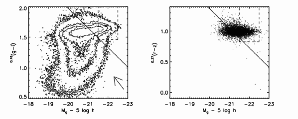
Figure 1.— Sample definition for the galaxies used in this paper. The left panel shows the low redshift selection regions; contours encapsulate 25%, 50%, 75%, and 95% of the considered galaxies. The right panels shows the target selection for our high-redshift galaxies overlayed on the LRG galaxies in the SDSS Southern Survey. In each panel, the solid line shows the selection cut which approximates a cut at constant stellar mass using the relations of Bell & de Jong (2000). The regions defined by the dashed lines were used to create control samples which do not have a strong cut across the red sequence to test the effects of sample selection on our scatter measurements. The arrow in the lower right of the left panel shows the reddening vector. Note the dearth of very luminous blue galaxies which could contaminate our red-sequence samples if heavily reddened.

2.2. Galaxy Photometric Properties

Several methods are used to measure galaxy fluxes in SDSS. Below, we briefly describe the two flux measurements used throughout this paper. The Petrosian ratio, ${{\mathcal{R}}_{P}}$, the ratio of the local surface brightness at radius $\theta$ to the average surface brightness at that radius, is given by

$${{\mathcal{R}}_{P}}(\theta)\equiv\frac{\left.\int_{\alpha_{\mathrm{lo}}\theta}^{\alpha_{\mathrm{hi}}\theta}d\theta^{\prime}2\pi\theta^{\prime}I(\theta^{\prime})\right/\left[\pi(\alpha_{\mathrm{hi}}^{2}-\alpha_{\mathrm{lo}}^{2})\theta^{2}\right]}{\left.\int_{0}^{\theta}dr^{\prime}2\pi\theta^{\prime}I(\theta^{\prime})\right/[\pi\theta^{2}]},$$ (1)

where $I(\theta)$ is the azimuthally averaged surface brightness profile of a galaxy and $\alpha_{\mathrm{lo}}$ and $\alpha_{\mathrm{hi}}$ are chosen to be 0.85 and 1.25 for SDSS. The Petrosian flux is given by the flux within a circular aperture of $2{{\theta}_{P}}$, where ${{\theta}_{P}}$ is the radius at which ${{\mathcal{R}}_{P}}$ falls below 0.2. In SDSS, ${{\theta}_{P}}$ is determined in the $r$ band then subsequently used in each of the other bands. This flux measurement contains a constant fraction of a galaxy’s light, independent of its size or distance, in the absence of seeing. More details of SDSS Petrosian magnitudes can be found in Blanton et al. (2001), and Strauss et al. (2002).

For each galaxy imaged by SDSS, two seeing-convolved models, a pure de Vaucouleurs (1948) profile and a pure exponential profile, are fit to the galaxy image. The best-fit model in the $r$ band is used to measure the flux of a galaxy in each of the other bands. These model magnitudes are unbiased in the absence of color gradients and provide higher signal-to-noise ratio colors than Petrosian colors. A more complete description of model magnitudes is given in Stoughton et al. (2002b). Throughout this paper, we use Petrosian magnitudes when calculating galaxy luminosities while model magnitudes are used to determine galaxy colors.

2.3. The $k$-Correction

We calculate photometric $k$-corrections using the method of Blanton et al. (2003c) (kcorrect v3_2). This program constructs a linear combination of carefully chosen spectral templates in order to best match the observed photometry at the measured redshift of the galaxy. The rest-frame colors of these best-fit spectra are used to derive corrections to the observed galaxy colors. With this method, it becomes simple to transform between bandpasses and, if necessary, photometric systems given a detailed understanding of the filter characteristics. After calculating $k$-corrections with kcorrect, we remove any mean $k$-corrected color versus redshift trends with a low order polynomial to account for the passive evolution of stellar populations between observed epochs. This evolutionary correction is normalized to a redshift of 0.3, near the median of the LRG redshift distribution. The color evolution correction is small (less than 2% for all bands in both samples) and does not affect any of the results presented here. We further assume a galaxy dims by one magnitude per $\Delta z=1$ change in redshift in the $g$-band due to the passive evolution of its stellar populations. Again, this correction is normalized to $z=0.3$. In the remainder of this paper, all of the color and luminosity measurements refer to quantities which have been adjusted for the $k$-correction and evolution.

Table 1Effective Wavelengths of Shifted Bandpasses

Filter	$\lambda_{\mbox{eff}}$
(1)	(2)
${}^{0.16}g$	4026
${}^{0.16}r$	5307
${}^{0.16}i$	6441
${}^{0.16}z$	7687
${}^{0.37}g$	3408
${}^{0.37}r$	4494
${}^{0.37}i$	5454
${}^{0.37}z$	6509

Throughout this paper, we work in the ${}^{0.16}g$, ${}^{0.16}r$, ${}^{0.16}i$, ${}^{0.16}z$ and ${}^{0.37}g$, ${}^{0.37}r$, ${}^{0.37}i$, ${}^{0.37}z$ systems for the low- and moderate-redshift galaxy samples, respectively. Here, the notation ${}^{z_{0}}g$ indicates the reported AB magnitudes are derived through a standard $g$ filter that has been blueshifted by $z_{0}$. For a filter system which has been shifted by $z_{0}$, the $k$-correction for galaxies at that redshift is trivial, $-2.5\,\mbox{log}\,(1+z_{0})$, and is independent of the galaxy spectral energy distribution. In choosing shifts which nearly match the median redshift of each sample, we minimize the uncertainty introduced through the $k$-corrections (Blanton et al. 2003c). Table 1 lists the effective wavelengths for each of the bandpasses used here.

2.4. Sample Construction

In order to investigate the color-magnitude relation of massive galaxies in the range $z\sim 0.1-0.4$, we create two samples from the SDSS spectroscopic database to be analyzed separately; Figure 1 shows the selection cuts used to define each of these samples. From the MAIN sample of galaxies, we extracted 16622 galaxies in the redshift range $0.1<z<0.2$ satisfying the rest-frame color cut

$${}^{0.16}(g-i)>8.374+0.32\left(M_{g}-5\,\hbox{log}\,h\right)$$ (2)

which approximates a cut of constant stellar mass (Bell & de Jong 2000). This selection criterion results in a cut diagonally across the red sequence, which could bias our measurements of the scatter in red sequence colors and will greatly affect any slope measurement of the color-magnitude relation. In order to avoid biased slope measurements and test the consistency of our scatter measurements, we also construct a sample of 5100 galaxies in the luminosity range $-22.5<M_{g}-5\,\hbox{log}\,h<-21.5$ with ${}^{0.16}(g-i)>1.46$ for comparison (shown by the dashed region in Figure 1).

We further select 2782 LRG galaxies from the SDSS Southern Survey in the redshift range $0.3<z<0.4$ which satisfy

$${}^{0.37}(r-z)>7.769+0.32\left(M_{g}-5\,\hbox{log}\,h\right)$$ (3)

and have been imaged 6 or more times. Equation 3 is the same rest-frame color cut applied to the low-redshift galaxies (Equation 2) shifted to the ${}^{0.37}(r-z)$ color — the effective wavelengths of the filters that define each of these colors are similar, and thus these colors probe similar regions in the rest-frame galaxy spectrum (see Table 1). Of these 2782 sample galaxies, 62% were imaged more than 9 times while 20% of the galaxies were imaged more than 12 times in the SDSS Southern Survey. As in the low-redshift sample, we adopt a simple constant color cut, ${}^{0.37}(r-z)>0.825$ and $-22.5<M_{g}-5\,\hbox{log}\,h<-21.5$, to define a subsample of 1380 high-redshift galaxies to test the consistency of our scatter measurements and allow us to determine the slope of the color-magnitude relation without a strong cut across the red sequence.

Figure 2.— Redshift distribution of the galaxies selected for this work is shown. The low-redshift sample was drawn from the MAIN SDSS galaxy sample while the moderate-redshift sample is composed of LRG galaxies selected from the SDSS Southern Survey. The low-redshift sample has robust photometry in one observation epoch as the galaxies are upwards of five magnitudes brighter than the SDSS detection limit while the higher redshift galaxies, which extended two magnitudes fainter, have been imaged repeatedly allowing for more precise photometric measurements.

We find no differences within our quoted error between the dispersion around the CMR measured from galaxies defined using the stellar mass cut and the constant color cut; throughout the remainder of this paper, scatter measurements will be based upon galaxies drawn in the first manner while all slope measurements are referenced to samples created using the latter method. Figure 2 shows the redshift distribution of the galaxies used to measure the scatter around the color-magnitude relation in this paper.

In detail, the red sequence is populated by elliptical and S0 galaxies as well as late-type galaxies reddened by dust. The arrow in the lower right of Figure 1 shows the reddening vector given by the O’Donnell (1994) extinction curve. In order for a dusty late-type galaxy to scatter into our sample, it must have a large unobscured luminosity as we only consider the most luminous red-sequence galaxies in this work. There is a clear paucity of very luminous blue galaxies in Figure 1 and thus the contamination from dusty spiral galaxies is likely small in our sample. Furthermore, Eisenstein et al. (2003) constructed the average spectrum of massive galaxies, such as those used in our analysis, and found that only 5% of the galaxy spectra in the $-22.5<M_{r}<-22$ luminosity range were contaminated by emission lines uncharacteristic of early-type galaxies. In the remainder of this paper, we will use the red-sequence and early-type classifications synonymously.

Throughout this paper, we will refer to the galaxies considered here as field galaxies as they are not specifically selected to reside in clustered environments. It is important to note, however, that galaxies which are of similar color and luminosity as those in our sample tend to lie in over-dense environments (Hogg et al. 2003). Zehavi et al. (2005) found the clustering strengths and mean separations of LRGs are comparable to those of poor clusters or rich groups. For comparison, of the LRGs in the volume surveyed by Bahcall et al. (2003) to find galaxy clusters with 13 or more detected cluster members, 16% are projected less than 500 kpc from the inferred location of a cluster and within 0.05 of the photometric redshift for that cluster. A detailed examination of the density dependence of the scatter around the CMR is conducted in §5.

Figure 3.— Measured slope of the CMR as a function of the rest-frame bandpass. The endpoints of the horizontal error bars mark the effective wavelengths of the filters used to define the bandpass while the vertical error bars show the measured uncertainty on each slope measurement. The spectrum of an early-type galaxy is plotted as a reference. The two symbols represents the two galaxy samples - the hollow squares mark measurements on the moderate-redshift ($0.3<z<0.4$) sample while the filled circles show the data from low-redshift (0.1 $<z<$ 0.2) galaxies.

3. The Color-Magnitude Relation

When determining the slope of the color-magnitude relation, we only consider the galaxies selected with our simple luminosity and constant color cuts as any slope measurements based on samples with a strong cut across the red sequence will be quite biased. The galaxy samples considered in this work only span a small range of luminosities and thus are not ideally suited for measurements of the slope of the CMR – we simply use our measurement of this quantity to remove the mean relationship before determining the scatter around it. The slopes and zero-points for the CMR for several colors are listed in Table 2. Figure 3 shows the measured slopes of the CMR as a function of the effective wavelengths of the two bandpasses used to define the color. The slope in bluer colors is more pronounced than that for redder bands which tend to show small or negligible slopes. This trend is consistent with a metallicity sequence as the primary driver along the red-sequence. As noted by Gladders et al. (1998) using models from Kodama (1997), the flattening of the color-magnitude relation toward redder colors can also be reproduced by an age trend along the red sequence but only if a very specific relationship between galaxy mass and star formation time holds with very little scatter. In the bluest colors, which have been used historically in the literature, the slopes measured here are in general agreement with past work; for comparison, Hogg et al. (2004) report a slope of $-0.022$ mag mag^-1 in the ${}^{0.1}(g-r)$ color for a large sample of galaxies at $z\sim 0.1$.

Table 2Slope of the Color-Magnitude Relation

	Total Sample			Field Sample			Cluster Sample
Color	Zero-point	Slope		Zero-point	Slope		Zero-point	Slope
	mag	mmag/mag		mag	mmag/mag		mag	mmag/mag
(1)	(2)	(3)		(4)	(5)		(6)	(7)
${}^{0.16}(g-r)$	1.162	$-15.6\pm 5.2$		1.162	$-10.5\pm 6.7$		1.164	$-12.4\pm 7.8$
${}^{0.16}(r-i)$	0.449	$-8.10\pm 2.6$		0.449	$-6.7\pm 3.4$		0.451	$-7.6\pm 4.3$
${}^{0.16}(i-z)$	0.329	$3.50\pm 6.4$		0.329	$4.2\pm 8.2$		0.329	$5.5\pm 10.4$
${}^{0.16}(g-i)$	1.611	$-26.1\pm 5.5$		1.610	$-21.5\pm 7.4$		1.612	$-22.9\pm 8.2$
${}^{0.37}(g-r)$	1.750	$-23.3\pm 12.1$		1.750	$-15.5\pm 16.1$		1.754	$-10.6\pm 19.5$
${}^{0.37}(r-i)$	0.613	$-3.8\pm 4.3$		0.612	$0.41\pm 6.2$		0.614	$-3.6\pm 8.4$
${}^{0.37}(i-z)$	0.379	$5.0\pm 6.1$		0.377	$0.58\pm 7.7$		0.381	$7.21\pm 9.9$
${}^{0.37}(r-z)$	0.991	$1.8\pm 8.5$		0.980	$3.4\pm 3.5$		0.983	$8.1\pm 1.4$

Figure 4.— Scatter around the color-magnitude relation for both galaxy samples. The ${}^{0.16}(r-i)$ and ${}^{0.37}(r-i)$ residual colors, normalized to the characteristic color of a galaxy with $M_{g}-5\,\mbox{log}\,h=-21.8$ are shown for the low and intermediate redshift galaxies respectively. Note that the dispersion of this relation is quite small. The dashed line is the best-fit Gaussian to the data. Table 3 lists the measured scatter around the CMR for all of the colors measured in this paper.

Figure 4 illustrates the typical scatter about the mean color-magnitude relation for the ${}^{0.16}(r-i)$ and ${}^{0.37}(r-i)$ colors; the measured dispersion about this relationship is quite small. The second column of Table 3 lists the measured dispersion around the CMR for each of the colors used in this study. For each color studied, we fit a Gaussian to the observed color distribution using Poisson errors on each color bin and define the dispersion of the best-fit Gaussian to be the scatter in galaxy colors on the red sequence. By fitting the histograms rather than calculating the standard deviation directly, we place more weight on the core of the distribution compared to the wings. Thus, our scatter measurements will not be heavily affected by any non-red-sequence interlopers in the wings of the color distributions. As this method could potentially depend on the binning used, we are careful to vary the bin size for each fit and ensure the measured scatter is not dependent on our choice of bin size. It should be noted that past work has used the standard deviation to quantify the scatter in galaxy colors. While the standard deviation and Gaussian widths may give systematically different dispersions in the case of non-Gaussian distributions, Figure 4 shows the color distribution on the red sequence is well described by a Gaussian and thus the two measurements are comparable. Bootstrap resampling of the data (e.g. Press 2002) was employed to determine the uncertainty on our scatter measurements. It is important to note that the scatter measurements in the second column of Table 3 represent upper limits to the intrinsic scatter in galaxy colors as these values are not corrected for systematic or experimental effects, which could be significant.

In order to investigate the level of skewness of the observed color distribution, we define $\beta_{n}$ to be the absolute value of the color difference between the $n\%$ quantile and the median of the distribution. The level of asymmetry in the distribution is then estimated using

$$\gamma=\frac{\beta_{10}-\beta_{90}}{\beta_{10}+\beta_{90}}.$$ (4)

For this statistic, a maximally skewed distribution would have $\gamma=\pm 1$ such that a tail of galaxies to the red would result in $\gamma<0$. A symmetric distribution would have $\gamma=0$. We adopt this approach rather than a traditional third moment calculation as the calculation of higher moments of a distribution is strongly dependent on the wings of the distribution where contamination may be important. For the histograms shown in Figure 4, we find that $\gamma=-0.027\pm 0.019$ for the ${}^{0.16}(r-i)$ color and $\gamma=-0.064\pm 0.048$ for the ${}^{0.37}(r-i)$ color. Both of these measurements reflect the slight over-abundance of red galaxies compared to a Gaussian in both panels of Figure 4. This red tail is due to the diagonal cut across the red sequence imposed by our stellar mass selction criterion; red galaxies are selected to lower luminosities than blue galaxies. Since the luminosity function of galaxies is steeply rising toward lower luminosities in this range, more red galaxies are selected than blue galaxies. For comparison, we measure $\gamma=0.001\pm 0.029$ for the ${}^{0.16}(r-i)$ color and $\gamma=-0.005\pm 0.057$ for the ${}^{0.37}(r-i)$ color when the simple luminosity cuts are used to select our sample galaxies.

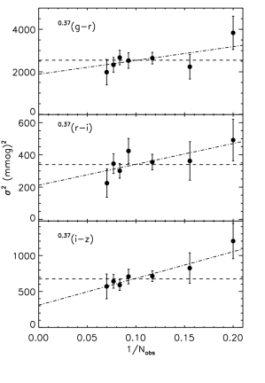
Figure 5.— Relationship between the number of observations and the measured scatter around the color-magnitude relation. The dotted line shows the weighted mean of the data while the dot-dashed line marks the best fit line to the data. The data for each color are not statistically consistent with a constant value but are well described by a line, as is expected. We extrapolate the best fit line to infinite measurements to find the intrinsic scatter in galaxy colors; these values are listed in the fourth column of Table 3.

Since our intermediate redshift sample is drawn from regions that have been repeatedly imaged by the Sloan Digital Sky Survey, we can assess the level to which the dispersion we observe in the color-magnitude relation is dependent on measurement noise. If the scatter is contaminated by measurement noise, we would expect the squared scatter to decrease inversely with the number of observations :

$$\sigma_{\rm obs}^{2}=\sigma_{\rm intrinsic}^{2}+\frac{A}{N_{\rm obs}}\,\,.$$ (5)

Figure 5 shows the results of this test; the methods used for the ensemble sample were used in the same manner to calculate the scatter and error for each bin. In each bin of $N$-measurements, we include galaxies which were imaged a total of $N$ times, and thus each bin contains a unique subsample of galaxies. For the moderate-redshift sample, the third and fourth columns in Table 3 lists the instrumental contribution and intrinsic galaxy scatter predicted by extrapolating the fits to Equation 2 to infinite observations for each of the three colors.

Table 3Scatter Around the Color-Magnitude Relation

Color	Measured Scatter	Instrumental Scatter	Intrinsic Scatter	Field	Clustered
	mmag	mmag	mmag	mmag	mmag
(1)	(2)	(3)	(4)	(5)	(6)
${}^{0.16}(g-r)$	$39.6\pm 0.4$	$17.6\pm 3.6$	$35.4\pm 3.7$	$40.5\pm 0.4$	$35.9\pm 0.8$
${}^{0.16}(r-i)$	$18.7\pm 0.2$	$15.1\pm 3.9$	$11.0\pm 4.0$	$19.1\pm 0.2$	$17.3\pm 0.3$
${}^{0.16}(i-z)$	$26.6\pm 0.4$	$20.9\pm 4.2$	$20.9\pm 4.2$	$26.7\pm 0.5$	$23.4\pm 0.8$
${}^{0.16}(g-i)$	$40.0\pm 0.4$	$21.2\pm 4.1$	$34.4\pm 4.1$	$42.0\pm 0.5$	$36.1\pm 0.7$
${}^{0.37}(g-r)$	$48.0\pm 1.2$	$20.4\pm 6.1$	$43.5\pm 6.2$	$48.8\pm 1.4$	$47.3\pm 2.2$
${}^{0.37}(r-i)$	$19.7\pm 0.5$	$12.3\pm 3.1$	$14.6\pm 3.1$	$20.1\pm 0.6$	$18.9\pm 1.0$
${}^{0.37}(i-z)$	$27.9\pm 0.7$	$21.6\pm 4.5$	$17.6\pm 4.6$	$29.2\pm 0.8$	$24.4\pm 1.4$
${}^{0.37}(r-z)$	$35.9\pm 1.1$	$18.4\pm 5.2$	$30.8\pm 5.2$	$38.1\pm 1.2$	$28.4\pm 2.1$

While the intrinsic dispersion around the color-magnitude relation at moderate redshift can be extracted from the measured scatter based on subsamples of galaxies with different number of measurements, the low-redshift galaxies do not allow for this test as most galaxies in this sample have been imaged only once. In order to estimate the intrinsic scatter in galaxy colors for this sample, we identified 5839 of our low-redshift galaxies that have been imaged more than once under photometric conditions. We adopt the average root-mean squared variation of each photometric measurement as the instrumental error for each color of interest. We find the mean measurement uncertainty to be 17.6, 15.1, and 20.9 mmag in the ${}^{0.16}(g-r)$, ${}^{0.16}(r-i)$, and ${}^{0.16}(i-z)$ bands, respectively. The internal dispersion in each color is the difference, in quadrature, between the measured scatter and inferred mean uncertainty in our single pass photometry. For the low-redshift galaxies, the third and fourth columns of Table 3 lists the observational error and intrinsic scatter determined by this correction. While our estimate of the instrumental contribution to the observed color dispersion corrects for uncorrelated errors on each independent measurement, we do not correct for systematic errors common to all observations which could cause an overestimation of the intrinsic dispersion in galaxy colors.

Figure 6.— Intrinsic scatter in the color-magnitude relation as a function of the observed bandpass. The error bars and symbols are defined as in Figure 3. The spectrum of an early-type galaxy is shown for comparison. The scatter in redder bands tends to be smaller than in blue bands. This is not unexpected, as small changes in a galaxy’s age, metallicity, or dust attenuation affect the blue portion of a its spectrum more than the red.

Figure 6 shows our scatter measurements as a function of the effective wavelength of the filters used to construct each color. The scatter about the CMR is clearly wavelength dependent; the bluest colors, which are most affected by small changes in the age, metallicity, or dust attenuation of the system, have systematically larger dispersions than the reddest colors where changes in metallicity and age have less impact.

4. Star Formation History of Massive Galaxies

Here, we consider three simple star formation histories and derive the range of permitted parameters for these histories following a method similar to that of van Dokkum et al. (1998). In these toy models, we will assume that only age variations between red-sequence galaxies creates the scatter in early-type galaxy colors. In reality, the scatter across the CMR is likely driven by some combination of age, metallicity, dust, and possibly $\alpha$-enhancement variations across the red-sequence. These models will thus illustrate the broadest range of ages allowed by our measurements; the inclusion of any variation in the other galaxy properties will only constrain the age more strongly.

In this section, we will primarily consider the high-redshift sample, as these are the intrinsically youngest galaxies in our sample and hence should provide the tightest constraints on the past star formation history of massive early-type galaxies. An identical analysis of the low-redshift sample provides results consistent with those presented below. In all three model cases, the low-redshift galaxies provide looser constraints than the high-redshift sample; star formation is allowed to continue to slightly later times.

First, we consider a star formation history composed of a single delta-function burst. The probability of a burst occurring is distributed uniformly between the earliest allowed time for galaxy formation, $t_{0}$, set to $z=10$, and $t_{\rm max}$, the time at which the youngest early-type galaxies form. Using a grid of Monte-Carlo simulations with 5000 galaxies per realization, we create samples of galaxy spectra synthesized using the method of Bruzual & Charlot (2003) with solar metallicity, a Salpeter (1955) initial mass function, and varying values of $t_{\rm max}$. We find that realizations allowing galaxies younger than 8.8 Gyr ($z\sim 1.4$) generate color distributions with standard deviations larger than that measured.

We perform a similar test using a scheme in which 80% of the stars in a galaxy are formed in a single burst at $z=10$ and 20% are formed in a second burst which occurs at a random time between $z=10$ and a minimum age, as done by van Dokkum et al. (1998). For this scenario, the secondary bursts must occur between $10>z>0.9$ to reconstruct the observed scatter in the color-magnitude relation. For bursts that generate less than 5% of a galaxy’s stars, the time scale for the secondary burst is unconstrained - small amounts of star formation can occur at late epochs without violating the constraints placed by our measurements.

Figure 7.— Reproduction of the observed scatter in rest-frame color of early-type galaxies using Monte-Carlo simulations following a method similar to that of van Dokkum et al. (1998). For each simulation, the top panel shows several examples of star formation histories drawn from the simulation. The shaded region denotes the allowed epoch of star formation for that simulation. Each of the bottom panels shows the distribution of residual colors around the color-magnitude relation for the realization that most closely matches the observed scatter. The $\gamma$ parameter, as defined in the text, is listed for each of the distributions. For comparison with the color distributions in Figure 4, we have added typical observational errors to the color distributions. The dashed line in each panel shows a Gaussian with the same mean and dispersion as the simulated colors. The left-most panel illustrates the allowed epoch of star formation for a SFH composed of a single delta function burst. For galaxy formation beginning at a redshift of 10, the youngest early-type galaxies must have formed by $z\sim 1.13$. The middle panel illustrates the allowed range of times for a secondary burst which contributes 20% of the stars to the galaxy. This secondary burst must have occurred before a $z\sim 0.84$. Finally, for a constant star formation history, all star formation must have ended by $z\sim 0.62$ to reproduce the observed scatter in the color-magnitude diagram at $z=0.37$. For reference, the lookback time at $z=0.37$ is 3.89 Gyr. A comparison with Figure 4 shows that the color distributions predicted by these models do not match the observed colors of massive galaxies, a sign that the models used here are overly simple. This is echoed by the mismatch between the $\gamma$ value measure from the data and those measured for each of the model distributions.

Finally, we create a grid of models in which star formation begins at $z=10$ and continues at a constant rate until it is truncated at $t_{\rm f}$. For each realization, we allow $t_{\rm f}$ to range from $z=10$ to a critical cutoff time at which all galaxies have stopped forming stars. Star formation in this manner must have ended by $z\sim 0.8$ in order to reproduce the observed scatter in the color-magnitude relation at $z=0.37$.

The allowed range of parameters and the distribution of galaxy colors found in each model are shown graphically in Figure 7. To allow comparison with Figure 4, typical observational errors have been included in the color distributions in the lower panels of the figure. Interestingly, all of these models predict similar scatter trends to those seen in Figure 6. In all three cases, the scatter in the ${}^{0.37}(g-r)$ color is nearly double that predicted for the ${}^{0.37}(r-i)$ and ${}^{0.37}(i-z)$ colors. While each of the three models succeeds in reproducing the observed scatter in early-type galaxy colors, none of the models adequately recreates the color distribution measured from real galaxies, a sign that the models chosen do not perfectly track the true evolution of the star formation history of early-type galaxies. The $\gamma$ parameter, as defined in Equation 4, for each of the model distributions is shown in Figure 7. The three models produce color distributions with $\gamma=(0.165,0.508,0.313)$ compared to the value of $-0.064$ calculated for the observed sample of galaxies at the same redshift. The difference between the observed skewness and that determined from our simple models reiterates the mismatch between the observed and predicted color distributions. In our simulations, we assume all galaxies have the same metallicity and no dust attenuation. Also, the onset of star formation is uniform in the second two models. In reality, these parameters are not constant, and thus the sharp truncations seen on the red edges of model color distributions will be blurred by the addition of other complications to the models. However, any of these corrections will increase the observed scatter in galaxy colors thus driving the last epoch of star formation needed to satisfy our constraints to earlier times.

5. Comparison with Clustered Environments

A majority of the work on the color-magnitude relation of early-type galaxies has focused on cluster galaxies at various redshifts. While some work (e.g. Sandage & Visvanathan 1978; Larson, Tinsley, & Caldwell 1980; Kodama, Bower, & Bell 1999) tackles the problem in the field, these studies suffer from small numbers of galaxies. The measurement of the scatter around the CMR presented here, on the other hand, focuses on the most massive field galaxies at moderate redshifts using a statistically significant sample. We can now, for the first time, statistically compare the dispersion around the CMR in both clustered and field environments.

In order to explore the environmental dependence of the color-magnitude relation within our data set, we use SDSS imaging of 5305 deg² to identify a comparison sample of 16 million normal galaxies down to $r=21$. At the location of each LRG galaxy in our sample, we count the number of neighboring galaxies within a $1\,h^{-1}$ Mpc (proper) aperture which have colors similar to those expected for an $L^{*}$ galaxy on the red sequence, and luminosities in the $M^{*}-0.5$ to $M^{*}+0.4$ range; the details of the luminosity and color cuts are given in Eisenstein et al. (2005).

Using the number of neighbor galaxies as a proxy for the environment of each LRG in our sample, we divide each of our galaxy sets into a clustered subsample and a low density subsample. We define LRG galaxies with more than 5 (7) neighboring galaxies in the low- (moderate-) redshift samples to be in clustered environments while a field subsample is comprised of galaxies with fewer neighbors. This threshold was chosen such that the clustered sample in both redshift bins composes 30% of the total galaxy sample at that redshift. To place these values in physical context, at $z=0.16$ ($z=0.37$) there are 25.3 (170) tracer galaxies per square degree. Given the angular diameter distance of 398 (712) $h^{-1}$ Mpc to that redshift, this yields a total of 1.65 (3.46) background galaxies per aperture on average. The average number of neighbors in the field sample is 2.3 (3.9) galaxies while the clustered galaxies have a mean of 9.1 (11.4) neighbors. Thus our clustered samples are over-dense by a factor of 4 (3) compared to the field galaxies.

Hogg et al. (2004) found that the slope and zeropoint of the color-magnitude relation do not depend strongly on the local galaxy environment. We find the same result; Table 2 lists the measurements of the slope and zeropoint of the relationship for the ensemble sample as well as for the field and clustered subsamples. The variation between the two samples is small. In the following calculations, we use the ensemble slope and zeropoint measurements as these are measured with the highest signal-to-noise. The results are unaffected if the individual measurements of the slope and zeropoint are used for each subsample.

The fifth and sixth columns of Table 3 list the measured scatter in galaxy colors for the field and clustered galaxies respectively. In all of the bands, the scatter for the field subsample is larger than that in clustered environments. If we assume the scatter introduced by instrumental effects is the same for both the field and clustered subsamples, the same correction determined for the ensemble galaxy sample can be applied to these subsamples, as well. With this correction, we find that the scatter in galaxy colors in dense environments is $11\pm 2\%$ smaller than for that of isolated systems in both redshift intervals studied here.

Our clustered galaxies reside in a range of densities, not simply rich clusters, as have often been used for similar studies, and thus we likely underestimate the significance of the difference in scatter between the field and strongly clustered environments. Furthermore, our field sample is not completely composed of isolated galaxies as the average number of neighbor galaxies in this sample is larger than the average density of background galaxies. Again, this leads to an underestimation of the true difference in the dispersion around the color-magnitude relation for field and clustered galaxies.

The larger scatter in field galaxy colors supports previous claims of an environmental dependence for the scatter around the color-magnitude relation for early-type galaxies (e.g. Larson, Tinsley, & Caldwell 1980; Kodama, Bower, & Bell 1999), though the effect measured here is weak. Comparisons of the scatter in galaxy colors for clustered galaxies often draw on galaxies from a single cluster whereas our clustered sample is created by combining galaxies from a number of clustered environments. It is possible that the star formation histories of galaxies in a single cluster are more highly coordinated than the star formation histories between different clusters, thus the scatter measured using galaxies from a single cluster would be smaller than when several clusters are combined. As the fraction of blue galaxies is larger in the field compared to clustered environments, the field subsample may have a larger contamination fraction compared the the clustered subsample. This would also cause an increased scatter in field galaxies colors compared to the galaxies in more dense environments.

Figure 8.— (a) Composite spectra of galaxies between 1-$\sigma$ and 3-$\sigma$ of the mean ${}^{0.16}(g-r)$ color. The gross properties of the composite red and blue spectra are quite similar. (b) The difference spectrum between the blue and red galaxies (middle) compared to the difference spectrum predicted for a passively evolving population (top) and an old population with a recent injection of young stars (bottom). The difference spectrum shows clear signs of enhanced Balmer absorption lines in the blue galaxies as well as stronger molecular features in the red galaxies. The red galaxies have stronger sodium absorption, leading to the “emission” feature in the difference spectrum. (c) Residuals between the data and comparison synthesis spectra. The general properties of the observed difference spectrum are matched in both comparisons, though the model consisting of an old galaxy with a small amount ($\sim 3\%$) of star formation in the past 1 Gyr slightly over-predicts the continuum strength in between 3900 Å and 4100 Å compared to the passively evolving model.

6. Average Galaxy Spectrum Across the Red Sequence

Having measured the scatter in galaxy colors, we next investigate the spectral differences between galaxies by examining the average spectrum of massive early-type galaxies across the red sequence. The composite early-type galaxy spectrum has been investigated as a function of environment, luminosity, redshift, size, and velocity dispersions (Eisenstein et al. 2003; Bernardi et al. 2003); here, we construct the composite spectrum for red sequence galaxies of different mean colors. Since the galaxies in our low-redshift sample are brighter, and thus have higher quality spectra, and are more numerous than the higher redshift galaxies, we only consider these galaxies in our analysis.

To construct the average spectrum of the galaxies in each color bin, we first shift the spectra according to the observed redshift and then normalize the observed SDSS spectrum by the flux at rest-frame 5000 Å. We augment the SDSS pixel mask to include all pixels within 10 Å of the bright sky lines at 5577, 5890, 5896, 6300, 6364, 7245, and 7283 Å. Since the galaxies of interest are in the redshift range $0.1<z<0.2$, the masked pixels occur at different rest-frame wavelengths for each galaxy, leaving the mean spectrum unaffected. We then find the number-weighted mean of the spectra, ignoring all masked pixels in the mean.

Galaxies are divided into two distinct color bins – red galaxies having ${}^{0.16}(g-r)$ colors between 1-$\sigma$ and 3-$\sigma$ redward of the mean and a blue sample in the same range blueward of the mean. The red galaxy bin contains 1321 galaxies with a mean ${}^{0.16}(g-r)$ color of 1.20 and $M_{g}-5\,\hbox{log}\,h=-21.3$ while the blue sample contains 1161 galaxies with mean color and luminosity of 1.09 and $M_{g}-5\,\hbox{log}\,h=-21.5$. Figure 8(a) shows the coadded spectra of the red and blue galaxies. The gross properties of each composite spectrum are similar. Figure 8(b) shows the difference between the blue and red spectra. This difference spectrum shows clear signs of enhanced Balmer absorption in the blue galaxies compared to the red composite, indicating that, on average, the blue galaxies contain more young stars, in agreement with past studies (e.g. Trager et al. 2000; Bernardi et al. 2005). While the red composite shows stronger [N II] emission lines relative to the blue composite, no other prominent emission lines, such as [O II], [O III], and H$\alpha$ are present; this emission line difference is likely due to a larger fraction of AGN in the red galaxies compared to the blue.

We consider two possible evolutionary scenarios to explain the spectral differences between the blue and red galaxies on the red sequence: pure age (i.e. passive) evolution of a single age stellar population and a recent epoch of star formation mixed with an existing old population. In the first scenario, we fit each composite spectrum with a solar metallicity, single age, stellar synthesis model created using the method of Bruzual & Charlot (2003). The red and blue spectra are best fit by 6.3 Gyr and 3.7 Gyr populations, respectively. In the second scenario, we find the blue composite spectrum is well fit by a 6.3 Gyr old stellar population mixed with a 1 Gyr population containing 3.5% of the stellar mass and we model the red composite with a simple 6.3 Gyr population. The difference spectra for both scenarios are shown in Figure 8(b). While each of the two model hypotheses would suggest quite different evolutionary histories for massive early-type galaxies, the predicted difference spectra are remarkably similar. The model consisting of a recent burst of star formation slightly over-estimates the continuum in the difference spectrum near 3900 Å and thus provides a marginally poorer fit to the data than the passive evolution model.

The residuals between the data and the model difference spectra are shown in Figure 8(c). Both of the models fail to match the strengths of the $\hbox{CN}_{2}$ and Mg $b$ features near 4140 and 5160 Å. Eisenstein et al. (2003) interpret these differences between observations and synthetic spectra as a enhanced $\alpha$-to-iron ratio present in the galaxies but not included in the synthetic models. Also, several weak iron features are evident in the two model spectra near 4300 and 5300 Å which are missing in the observed difference spectrum. In a pure-age model for the evolution across the red sequence, the enhanced blue continuum provided by the hotter stars in the young population dilutes the metal lines seen in the older population. This dilution leads to differences in the strengths of the metal lines of the two population models, thus causing the residual iron features in both model difference spectra. The absence of these residuals in our observed difference spectrum indicates that a pure-age model for the spectral differences between red and blue galaxies on the red sequence is an incomplete model. In order to match the variations of the spectral features across the red sequence, a more detailed model is required. This model should include both age and metallicity variation and, more importantly, non-solar abundance ratios. Until spectral synthesis models with realistic $\alpha$-enhancement prescriptions are available, more quantitative analysis of our observed difference spectrum is difficult as the interplay between age, metallicity, and $\alpha$-to-iron ratio variations must be included for a full understanding of the physical differences between these galaxies.

Another clear difference between the models and the data is the strong Na D feature near 5892 Å. Here, the red composite spectrum has considerably more Na D absorption than predicted by the stellar synthesis models. As the model spectra do not contain absorption due to the interstellar medium, this discrepancy may indicate that the red galaxies contain more neutral gas than their blue counterparts.

7. Conclusions

We present new multi-color observations of a large sample of galaxies in the range $0.1<z<0.4$ gathered from the Sloan Digital Sky Survey. These galaxies represent the most massive galaxies in the Universe and are not selected to be in clustered environments. Past studies of the color-magnitude relationship have focused on $L^{*}$ galaxies in clusters, thus our work focuses on an area of parameter space previously unexplored. Using the robust photometry of bright galaxies provided by the SDSS as well as multiple observations of moderate-redshift galaxies, we are able to construct the color-magnitude relations for massive field galaxies in several colors. While our data only span one magnitude in luminosity, and thus are not ideal for in-depth analysis of the slope and zeropoint of the CMR, our large sample of galaxies allows us to measure the dispersion about this relationship quite well. The scatter around the red sequence is 20 mmag in the reddest bands while the bluest colors have nearly double this value.

We construct several toy model star formation histories in order to place constraints on the evolutionary processes at work in massive galaxies. We find that the majority of star formation in these early-type galaxies must have occurred before $z\sim 1$, in agreement with other authors. For secondary bursts of star formation with strengths less than 5% of the total stellar mass of the system, our data are consistent with bursts of star formation at any epoch. However, one should note that none of the toy models reproduce the observed distribution of galaxy colors.

Furthermore, we make comparisons between our new measurement of the scatter around the color-magnitude relation for massive field galaxies and early-type galaxies in clusters. An internal comparison shows that the scatter around the CMR in dense environments is $11\pm 2\%$ smaller than that measured using more isolated galaxies.

The composite spectra of LRG galaxies redward and blueward of the mean galaxy color are physically distinct. The blue galaxies show stronger Balmer absorption than the red galaxies, consistent with the presence of a younger stellar population. Simple models slightly favor passive evolution of stellar populations as the cause of the observed differences in spectra across the red sequence compared to a more recent injection of young stars onto an old stellar population, though the difference between the predicted spectra from these models is small.

8. Acknowledgments

We would like to thank Michael Blanton, Scott Burles, Douglas Finkbeiner, David Hogg, David Schlegel, John Moustakas, Amelia Stutz, and Jane Rigby for software and helpful comments during the preparation of this paper. We further thank the anonymous referee for a thorough and critical reading of our paper which lead to substantial improvements to the text. This research made use of the NASA Astrophysics Data System. RJC is funded through a National Science Foundation Graduate Research Fellowship. DJE is supported by NSF grant AST 339020 and an Alfred P. Sloan Research Fellowship.

Funding for the creation and distribution of the SDSS Archive has been provided by the Alfred P. Sloan Foundation, the Participating Institutions, the National Aeronautics and Space Administration, the National Science Foundation, the U.S. Department of Energy, the Japanese Monbukagakusho, and the Max Planck Society. The SDSS Web site is http://www.sdss.org/.

The SDSS is managed by the Astrophysical Research Consortium (ARC) for the Participating Institutions. The Participating Institutions are The University of Chicago, Fermilab, the Institute for Advanced Study, the Japan Participation Group, The Johns Hopkins University, the Korean Scientist Group, Los Alamos National Laboratory, the Max-Planck-Institute for Astronomy (MPIA), the Max-Planck-Institute for Astrophysics (MPA), New Mexico State University, University of Pittsburgh, University of Portsmouth, Princeton University, the United States Naval Observatory, and the University of Washington.

References

- Abazajian et al. (2003) Abazajian, K., et al. 2003, AJ, 126, 2081
- Abazajian et al. (2004a) Abazajian, K., et al. 2004, AJ, 128, 502
- Abazajian et al. (2005) Abazajian, K., et al. 2005, AJ, 129, 1755
- Andreon (2003) Andreon, S. 2003, A&A, 409, 37
- Arimoto & Yoshii (1987) Arimoto, N. & Yoshii, Y. 1987, A&A, 173, 23
- Bahcall et al. (2003) Bahcall, N. A., et al. 2003, ApJS, 148, 243
- Baldry et al. (2004) Baldry, I. K., Glazebrook, K., Brinkmann, J., Ivezić, Ž., Lupton, R. H., Nichol, R. C., & Szalay, A. S. 2004, ApJ, 600, 681
- Bell & de Jong (2000) Bell, E. F., & de Jong, R. S. 2000, MNRAS, 312, 497
- Bernardi et al. (2003) Bernardi, M., et al. 2003, AJ, 125, 1882
- Bernardi et al. (2005) Bernardi, M., Sheth,R. K., Nichol, R. C., Schneider, D. P., & Brinkmann, J. 2005, AJ, 129, 61
- Blakeslee et al. (2003) Blakeslee, J. P., et al. 2003, ApJ, 596, L143
- Blanton et al. (2001) Blanton, M. R., et al. 2001, AJ, 121, 2358
- Blanton et al. (2003a) Blanton, M. R., et al. 2003, ApJ, 594, 186
- Blanton et al. (2003b) Blanton, M. R., Lin, H., Lupton, R. H., Maley, F. M., Young, N., Zehavi, I., & Loveday, J. 2003, AJ, 125, 2276
- Blanton et al. (2003c) Blanton, M. R., et al. 2003,AJ, 125, 2348
- Bower, Lucey, & Ellis (1992) Bower, R. G., Lucey J. R., & Ellis, R. S. 1992, MNRAS, 254, 601
- Bressan, Chiosi, & Tantalo (1996) Bressan, A., Chiosi, C., & Tantalo, R. 1996, A&A, 311, 425
- Bruzual & Charlot (2003) Bruzual, G. & Charlot, S. 2003, MNRAS, 344, 1000
- De Lucia et al. (2005) De Lucia, G., Springel, V., White, S. D. M., Croton, D., & Kauffmann, G. 2005, ArXiv Astrophysics e-prints, arXiv:astro-ph/0509725
- de Vaucouleurs (1948) de Vaucouleurs, G. 1948, Annales d’Astrophysique, 11, 247
- Eisenstein et al. (2005) Eisenstein, D. J., Blanton, M., Zehavi, I., Bahcall, N., Brinkmann, J., Loveday, J., Meiksin, A., & Schneider, D. 2005, ApJ, 619, 178
- Eisenstein et al. (2003) Eisenstein, D. J., et al. 2003, ApJ, 585, 694
- Eisenstein et al. (2001) Eisenstein, D. J., et al. 2001, AJ, 122, 2267
- Ellis et al. (1997) Ellis, R. S., Smail, I., Dressler, A., Couch, W. J., Oemler, A. J., Butcher, H., & Sharples, R. M. 1997, ApJ, 483, 582
- Faber (1972) Faber, S. M. 1972, A&A, 20, 361
- Faber (1973) Faber, S. M. 1973, ApJ, 179, 731
- Fukugita et al. (1996) Fukugita, M., Ichikawa, T., Gunn, J. E., Doi, M., Shimasaku, K., & Schneider, D. P. 1996, AJ, 111, 1748
- Gladders et al. (1998) Gladders, M. D., Lopez-Cruz, O., Yee, H. K. C., & Kodama, T. 1998, ApJ, 501, 571
- Gunn et al. (1998) Gunn, J. E., et al. 1998, AJ, 116, 3040
- Hogg, et al. (2001) Hogg, D. W., Finkbeiner, D. P., Schlegel, D. J., & Gunn, J. E. 2001, AJ, 122, 2129
- Hogg et al. (2003) Hogg, D. W., et al. 2003, ApJ, 585, L5
- Hogg et al. (2004) Hogg, D. W., et al. 2004,ApJ, 601, L29
- Ivezić et al. (2004) Ivezić, Ž., et al. 2004, Astronomische Nachrichten, 325, 583
- Kauffmann & Charlot (1998) Kauffmann, G. & Charlot, S. 1998, MNRAS, 294, 705
- Kodama (1997) Kodama, T. 1997, Ph.D. thesis, Univ. Tokyo
- Kodama & Arimoto (1997) Kodama, T. & Arimoto, N. 1997, A&A, 320, 41
- Kodama, Bower, & Bell (1999) Kodama, T., Bower, R. G., & Bell, E. F. 1999, MNRAS, 306, 561
- Larson (1974) Larson, R. B. 1974, MNRAS, 166, 585
- Larson, Tinsley, & Caldwell (1980) Larson,R. B., Tinsley, B. M., & Caldwell, C. N. 1980, ApJ, 237, 692
- Lugger (1984) Lugger, P. M. 1984, ApJ, 278, 51
- López-Cruz, Barkhouse, & Yee (2004) López-Cruz, O., Barkhouse, W. A., & Yee, H. K. C. 2004, ApJ, 614, 679
- Lupton et al. (2001) Lupton, R. H., Gunn, J. E., Ivezić, Z., Knapp, G. R., Kent, S., & Yasuda, N. 2001, ASP Conf. Ser. 238:Astronomical Data Analysis Software and Systems X, 10, 269
- Lupton et al. (1999) Lupton, R. H., Gunn, J. E., & Szalay, A. S. 1999, AJ, 118, 1406
- Matteucci & Tornambe (1987) Matteucci, F. & Tornambe, A. 1987, A&A, 185, 51
- McIntosh et al. (2005) McIntosh, D. H., Zabludoff, A. I., Rix, H., & Caldwell, N. 2005, ApJ, 619, 193
- O’Connell (1980) O’Connell, R. W. 1980, ApJ, 236, 430
- O’Donnell (1994) O’Donnell, J. E. 1994, ApJ, 422, 158
- Pier et al. (2003) Pier, J. R., Munn, J. A., Hindsley, R. B., Hennessy, G. S., Kent, S. M., Lupton, R. H., & Ivezić, Ž. 2003, AJ, 125, 1559
- Press (2002) Press, W. H. 2002, Numerical recipes in C++ : the art of scientific computing by William H. Press. xxviii, 1,002 p. : ill. ; ISBN : 0521750334,
- Rose (1985) Rose, J. A. 1985, AJ, 90, 1927
- Salpeter (1955) Salpeter, E. E. 1955, ApJ, 121, 161
- Sandage & Visvanathan (1978) Sandage, A. & Visvanathan, N. 1978, ApJ, 225, 742
- Schlegel et al. (1998) Schlegel, D. J., Finkbeiner, D. P., & Davis, M. 1998, ApJ, 500, 525
- Smith et al. (2002) Smith, J. A., et al. 2002, AJ, 123, 2121
- Stoughton et al. (2002) Stoughton, C., et al. 2002, AJ, 123, 485
- Stoughton et al. (2002b) Stoughton, C., et al. 2002, Proc. SPIE, 4836, 339
- Strauss et al. (2002) Strauss, M. A., et al. 2002, AJ, 124, 1810
- Terlevich et al. (1999) Terlevich, A. I., Kuntschner, H., Bower, R. G., Caldwell, N., & Sharples, R. M. 1999, MNRAS, 310, 445
- Terlevich, Caldwell, & Bower (2001) Terlevich, A. I., Caldwell, N., & Bower, R. G. 2001, MNRAS, 326, 1547
- Trager et al. (2000) Trager, S. C., Faber,S. M., Worthey, G., & González, J. J. 2000, AJ, 119, 1645
- van Dokkum et al. (1998) van Dokkum, P. G.,Franx, M., Kelson, D. D., Illingworth, G. D., Fisher, D., & Fabricant, D. 1998, ApJ,500, 714
- van Dokkum et al. (2000) van Dokkum, P. G., Franx, M., Fabricant, D., Illingworth, G. D., & Kelson, D. D. 2000, ApJ, 541, 95
- van Dokkum et al. (2001) van Dokkum, P. G., Stanford, S. A., Holden, B. P., Eisenhardt, P. R., Dickinson, M., & Elston, R. 2001,ApJ, 552, L101
- Visvanathan & Sandage (1977) Visvanathan, N. & Sandage, A. 1977, ApJ, 216, 214
- Worthey et al. (1995) Worthey, G., Trager, S. C., & Faber, S. M. 1995, ASP Conf. Ser. 86: Fresh Views of Elliptical Galaxies, 86, 203
- York et al. (2000) York, D. G., et al. 2000, AJ, 120, 1579
- Zehavi et al. (2005) Zehavi, I., et al. 2005, ApJ, 621, 22
- Zepf, Whitmore, & Levison (1991) Zepf, S. E., Whitmore, B. C., & Levison, H. F. 1991, ApJ, 383, 524