ChaMPlane Optical Survey: Mosaic Photometry

Abstract

The ChaMPlane survey to identify and analyze the serendipitous X-ray sources in deep Galactic plane fields incorporates the ChaMPlane Optical Survey, which is one of NOAO’s Long-term Survey Programs. We started this optical imaging survey in March 2000 and completed it in June 2005. Using the NOAO 4-m telescopes with the Mosaic cameras at CTIO and KPNO, deep images of the ChaMPlane fields are obtained in V, R, I and H$\alpha$ bands. This paper describes the process of observation, data reduction and analysis of fields included in the ChaMPlane Optical Survey, and describes the search for H$\alpha$ emission objects and Chandra optical counterparts. We illustrate these procedures using the ChaMPlane field for the black hole X-ray binary GRO J0422+32 as an example.

1. Introduction

The ChaMPlane Survey identifies serendipitous X-ray sources located to arcsec precision in the Galactic plane fields from the Chandra archive, in order to determine the populations of accretion-powered binaries in the Galaxy (Grindlay et al. (2005), and see Grindlay et al. (2003); Zhao et al. (2003) for early descriptions).

The primary goals of this survey are: 1) to identify Cataclysmic Variables (CVs) and quiescent Low Mass X-ray Binaries (qLMXBs: which contain either black hole or neutron star primaries) in order to measure their number and space density luminosity functions; and 2) to determine the distributions of High Mass X-ray Binaries with Be star secondaries. The secondary goal is to study the distributions of stellar coronal source and diffuse X-ray objects in the Galactic Plane. See Grindlay et al. (2005) for a complete description of the survey goals, selection criteria and initial results.

ChaMPlane consists of an X-ray and an Optical survey. The X-ray survey, supported by NASA through Chandra archival proposals, searches for X-ray sources detected serendipitously in Chandra archival fields. In the Optical Survey, supported by NOAO, we look for H$\alpha$ emission sources and the Chandra optical counterparts in 4-meter telescope Mosaic images taken at CTIO and KPNO. We successfully conducted the ChaMPlane Optical Survey from March 2000 to June 2005. This 5 year survey produced 65 Mosaic fields covering about 23 square degrees and 154 ACIS observations on 105 distinct Chandra fields (defined as groups of individual observations whose aimpoints are $\geqslant$4′ apart) in the Galactic plane during Chandra Cycles 1-6.

In this paper we describe the methods of the ChaMPlane Optical Survey and the procedures to search for H$\alpha$ emission objects and Chandra optical counterparts. Section 2 describes the observational approach. Section 3 describes the Mosaic data reduction. Section 4 describes the photometric analysis and calibration. Section 5 describes the photometric results – the optical catalog. Section 6 gives the astrometric accuracy of the catalog. Sections 7 and 8 describe the search for H$\alpha$ emission objects and Chandra optical counterparts, respectively. Section 9 describes the data product, and uses the results from the GRO J0422+32 field as an example.

2. Optical Imaging

Under the NOAO Long-term Survey Program, we were granted 5 nights CTIO 4-m and 1-2 nights KPNO 4-m telescope time each year for 5 years. Before this long term program officially started in December 2000 at KPNO, we conducted a pilot run using the CTIO 4-m Mosaic on March 13-15, 2000. Under this Survey Program, we are committed to establish an archival database to provide the community with all of our optical images as well as a photometrically-calibrated star catalog.

ChaMPlane fields are selected from the Chandra target list based on criteria given in Grindlay et al. (2005). Deep optical imaging is the crucial first step of the ChaMPlane survey. It serves two purposes: 1) to identify candidate optical counterparts of the Chandra sources and to measure their optical magnitudes and $F_{X}/F_{opt}$ ratios for approximate spectral classification and constraints on reddening; and 2) to identify CVs and qLMXBs by their ubiquitous H$\alpha$ excess as “blue” objects in the R vs. (H$\alpha-$ R) diagram. It also paves the way for the next step – spectroscopic follow-up for classification on identified ChaMPlane objects.

2.1. Instrument

The images were taken with the Mosaic-I (KPNO) and Mosaic-II (CTIO) cameras. The Mosaic camera is a 8k$\times$8k CCD array, which consists of eight 2048$\times$4096 SITe CCDs. The pixel size is 15 $\mu$m (0.26$\arcsec$ at the 4-m telescope), which gives adequate resolution. It provides a field of view of 36$\arcmin\times$36$\arcmin$, which covers the full Chandra/ACIS FoV. Images were taken with filters of Johnson V, R, I and H$\alpha$ (80Å FWHM centered on the H$\alpha$ line).

To prepare the observation, the center of each Mosaic field (i.e. the telescope pointing) was carefully positioned so that the Mosaic covers all the active ACIS chips (typically, six ACIS chips are turned on). For the Mosaic fields covering multiple Chandra observations, their centers were positioned so that the Mosaic can cover maximum numbers of active ACIS chips possible.

2.2. Observations

Table 1 lists all the ChaMPlane Optical Imaging runs conducted. Table 2 is a complete list of all 65 observed ChaMPlane Mosaic fields. The name of each field is based on the main Chandra observation covered by that Mosaic field, except for fields GC1 – GC6, which are our Galactic Center mapping of 2.2 square degrees that covers 58 Chandra ACIS observations in Cycles 1-6 (including 20 SgrA* (Muno et al., 2003), 30 Galactic Center Survey (Wang et al., 2002) and 8 other observations in the Galactic Center region). Figure 1 shows these 65 fields in Galactic coordinates.

Table 1ChaMPlane Observations: Mosaic Imaging

Code	Telescope	Observing Date	Fields
ctio00	CTIO 4-m	Mar. 13 – 15, 2000	9
kpno00	KPNO 4-m	Dec. 5 –  6, 2000	4
ctio01	CTIO 4-m	May 13 – 17, 2001	8
kpno01	KPNO 4-m	Oct. 25, 2001	3
kpno02	KPNO 4-m	Dec. 7 –  8, 2002	6
ctio03	CTIO 4-m	Jun. 2 –  6, 2003	11
kpno03	KPNO 4-m	Jan. 30 – 31, 2004	2
ctio04	CTIO 4-m	May 16 – 20, 2004	13
kpno04	KPNO 4-m	Jan. 11 – 12, 2005	3
ctio05	CTIO 4-m	Jun. 7 – 11, 2005	6
Total			65

Table 2 65 ChaMPlane Mosaic Fields (sorted by RA)

N	Code	Field	RA(J2000)	Dec(J2000)	$l~{}(^{\circ})$	$b~{}(^{\circ})$	N${}_{\rm H}/10^{22}$
26	kpno02	G127.1$+$0.5	01:28:00.00	$+$63:03:11.7	127.06023	0.47507	0.869
58	kpno04	MAFFEI1	02:36:49.80	$+$59:36:19.0	135.90926	$-$0.58435	0.591
11	kpno00	GKPERSEI	03:30:37.89	$+$43:51:15.8	150.90053	$-$10.20409	0.181
12	kpno00	GROJ0422$+$32	04:21:20.40	$+$32:55:37.9	165.81091	$-$11.95536	0.189
13	kpno00	NGC1569	04:30:25.00	$+$64:44:53.0	143.72842	11.14309	0.412
23	kpno01	3C123	04:36:28.00	$+$29:37:49.0	170.52481	$-$11.78690	0.659
42	kpno03	AFGL618	04:42:23.39	$+$36:04:35.3	166.40825	$-$6.62965	0.462
24	kpno01	3C129	04:49:19.20	$+$45:02:30.0	160.42311	0.18431	0.644
27	kpno02	G166.0$+$4.2	05:27:12.06	$+$42:54:05.1	166.21402	4.36698	0.378
28	kpno02	PSRJ0538$+$2817	05:38:00.54	$+$28:14:24.0	179.70937	$-$1.78641	0.759
43	kpno03	1SAXJ0618.0$+$2227	06:18:18.70	$+$22:29:20.8	189.24487	3.20883	1.045
1	ctio00	A0620$-$00	06:23:15.70	$-$00:18:20.7	209.98050	$-$6.40597	0.292
29	kpno02	MADDALENA’SCLOUD	06:49:24.78	$-$04:34:07.2	216.77023	$-$2.53092	0.944
30	kpno02	M1$-$16	07:37:14.89	$-$09:41:07.6	226.82573	5.59410	0.130
59	kpno04	OH231.8$+$4.2	07:42:01.49	$-$14:45:18.0	231.84038	4.14583	0.428
2	ctio00	PKS0745$-$191	07:47:16.70	$-$19:15:05.0	236.37517	3.00117	0.306
3	ctio00	NGC3256	10:28:41.70	$-$43:59:18.3	277.54922	11.73626	0.068
14	ctio01	V382VELORUM1999	10:44:48.00	$-$52:18:18.0	284.10977	5.87716	0.258
60	ctio05	PSRB1046$-$58	10:48:00.00	$-$58:28:48.0	287.37619	0.61334	0.684
31	ctio03	MSH11$-$62	11:11:57.38	$-$60:41:28.0	291.05115	$-$0.13479	0.637
15	ctio01	NGC3603	11:15:49.80	$-$61:17:23.0	291.70792	$-$0.51893	16.683
32	ctio03	G292.2$-$0.5	11:19:45.94	$-$61:40:13.5	292.28198	$-$0.70890	2.162
33	ctio03	CENX$-$3	11:20:49.67	$-$60:37:04.3	292.03949	0.32333	0.665
61	ctio05	MYCN18	13:39:57.60	$-$67:20:24.0	307.59271	$-$4.90835	0.317
44	ctio04	G309.8$+$0.0	13:50:12.00	$-$62:09:36.0	309.73349	$-$0.06672	7.336
45	ctio04	PSRJ1509$-$5850	15:09:36.00	$-$58:48:18.0	320.01083	$-$0.59235	6.358
46	ctio04	G322.5$-$0.1	15:24:00.00	$-$57:06:53.2	322.52438	$-$0.16385	4.416
16	ctio01	4U1538$-$52	15:42:01.40	$-$52:18:22.0	327.42334	2.26117	1.319
47	ctio04	XTEJ1550$-$564	15:51:01.07	$-$56:27:16.6	325.90033	$-$1.81329	0.944
62	ctio05	ABELL3627	16:13:45.60	$-$60:48:36.0	325.24203	$-$7.03382	0.121
34	ctio03	1RXSJ161411.3$-$630657	16:14:53.00	$-$63:12:57.0	323.64777	$-$8.85384	0.075
48	ctio04	MZ3	16:17:09.70	$-$51:59:30.2	331.71680	$-$1.00867	1.132
4	ctio00	GROJ1655$-$40	16:54:28.90	$-$39:51:31.7	345.02972	2.37637	0.638
49	ctio04	MARS	17:00:48.53	$-$26:58:24.2	356.04932	9.28549	0.132
50	ctio04	XTEJ1709$-$267	17:09:36.71	$-$26:36:53.0	357.51978	7.91659	0.341
17	ctio01	PSRB1706$-$44	17:09:42.00	$-$44:30:45.0	343.07489	$-$2.69993	1.319
5	ctio00	G347.5$-$0.5a	17:12:16.10	$-$39:34:39.6	347.33688	$-$0.16436	4.895
6	ctio00	G347.5$-$0.5b	17:15:36.00	$-$39:58:36.0	347.38821	$-$0.91690	1.794
51	ctio04	TORNADO	17:40:00.00	$-$30:57:59.2	357.63300	$-$0.03307	11.271
35	ctio03	GC5	17:43:04.80	$-$29:37:48.0	359.11887	0.10892	15.853
36	ctio03	GC2	17:43:33.12	$-$29:01:48.0	359.68350	0.33651	4.930
37	ctio03	GC3	17:45:44.88	$-$28:25:48.0	0.44666	0.23978	17.838
38	ctio03	GC6	17:45:49.20	$-$29:37:48.0	359.43039	$-$0.39852	10.212
7	ctio00	SGRA*	17:46:11.20	$-$28:53:52.0	0.09729	$-$0.08582	54.518
39	ctio03	GC1	17:46:16.32	$-$29:01:48.0	359.99405	$-$0.17051	36.045
8	ctio00	SGRB2	17:46:43.10	$-$28:29:42.1	0.50199	0.02380	65.053
9	ctio00	GALACTICCENTERARC	17:47:08.60	$-$28:53:36.0	0.20979	$-$0.26248	20.284
40	ctio03	GC4	17:48:27.60	$-$28:25:48.0	0.75573	$-$0.27009	30.783
63	ctio05	LIMITINGWINDOW	17:51:48.00	$-$29:34:12.0	0.15160	$-$1.48171	0.704
52	ctio04	STANEKWINDOW	17:54:24.42	$-$29:49:16.3	0.22242	$-$2.09703	0.478
53	ctio04	4U1755$-$33	17:58:49.20	$-$33:51:00.0	357.19409	$-$4.92093	0.399
18	ctio01	PSRB1757$-$24	18:01:48.00	$-$24:49:39.0	5.37027	$-$1.02458	4.030
54	ctio04	BAADE’SWINDOW	18:03:36.00	$-$29:57:50.7	1.08909	$-$3.89739	0.321
55	ctio04	G11.4$-$0.1	18:11:20.40	$-$19:14:24.0	11.32621	$-$0.22863	8.865
19	ctio01	PSR1813$-$36	18:16:25.00	$-$36:20:29.5	356.70163	$-$9.27033	0.092
64	ctio05	V4641SGR	18:19:21.38	$-$25:27:00.0	6.73546	$-$4.80812	0.289
56	ctio04	PSRB1823$-$13	18:26:00.00	$-$13:37:12.0	17.94011	$-$0.66268	7.538
20	ctio01	MWC297	18:27:59.80	$-$03:51:02.6	26.82325	3.44240	6.963
41	ctio03	GALACTICPLANE	18:43:27.72	$-$03:58:12.0	28.49013	$-$0.03869	17.281
21	ctio01	SGR1900$+$14	19:07:38.30	$+$09:18:08.1	43.04858	0.66903	2.784
65	ctio05	1H1905$+$000	19:08:36.00	$+$00:11:24.0	35.06054	$-$3.73080	0.359
10	kpno00	B2224$+$65	22:25:13.22	$+$65:32:45.2	108.55382	6.84190	0.460
22	kpno01	3EGJ2227$+$6122	22:29:17.00	$+$61:19:00.9	106.70962	3.00593	1.012
57	kpno04	CTB$-$109LOBE	23:02:18.85	$+$58:54:40.1	109.23905	$-$1.02858	1.032
25	kpno02	G116.9$+$0.2	23:59:12.53	$+$62:24:00.0	116.92374	0.13922	0.461

Figure 1.— Observed ChaMPlane Mosaic fields in Galactic coordinates. Several fields in the Galactic center region are unresolved on this figure (see Grindlay et al. (2005) for an expanded view of the galactic center region fields.).

Exposure times were targeted to obtain “shallow” exposures to sample the bright sources in the field and “deep” exposures to reach the survey goal of $\sim$24 mag for 5% photometry in the R filter and 10% photometry in the other filters. This is to ensure that our primary measurement of H$\alpha-$R, to search for H$\alpha$ bright optical counterparts, is not compromised by limited sensitivity in the narrow-band H$\alpha$ filter. This sensitivity limit is computed assuming average seeing ($\sim 1.0\arcsec$), airmass ($\sim$1.2), and lunar phase ($\sim$4 days). Shallow exposures were 2 seconds for each of the V, R, I filters and 30 seconds for the H${\alpha}$ filter; deep exposures were 900 seconds each for V and I, 1200 seconds for R, and 7500 seconds for H${\alpha}$. Each of the long exposures were divided into 5 dithered sub-exposures to prevent chip gaps and bad columns in the data and to provide cosmic-ray rejection. Stars usually saturate at $\sim$12 mag in the shallow images and $\sim$17 mag in the deep ones. Considering overhead time at the telescope, each field takes 3.5 – 4 hours, allowing us to observe three fields per night. Absolute minimal observations require the deep R and H${\alpha}$ exposures.

Standard calibration images (biases, dome flats) are taken at the telescope daily before observing. Ideal sky flats are usually constructed from object frames after eliminating all the stars. In the Galactic plane, however, the stellar density is too high for this process, so instead we obtained twilight flats. Sky flats are critically important for the I and H$\alpha$ images from the KPNO 4-m to remove a pupil ghost caused by light back-scattered from the telescope optics that affects the four inner Mosaic CCDs. Dark images are not needed for this project as the dark current is very low ($\sim 5e^{-}$/pixel/hr for Mosaic-I and $\sim<2e^{-}$/pixel/hr for Mosaic-II).

3. Mosaic Data Reduction

The data reduction of Mosaic images is done using the Mosaic Data Reduction package (MSCRED) of IRAF. This section summarizes our reduction process, relying heavily on the detailed reduction description of Jannuzi et al. for the NOAO Deep Wide Field Survey.

3.1. CCD reduction

The raw data are reduced using the IRAF/mscred/ccdproc package, including standard CCD corrections. For the Mosaic-II data, the data from the two amplifiers of the same CCD are merged. The Mosaic-I images are affected by the pupil ghost described in the Mosaic User Manual and the sky flats are used to remove the ghost at this juncture. Each reduced image is then processed to remove cosmic rays and to fix the bad pixels and columns.

3.2. Astrometry

Astrometry was performed on each image using IRAF/mscred/msccmatch which allows for zero-point shifts, scale changes, and axis rotations. It also corrects for atmospheric refraction effects. Of the two World Coordinate System (WCS) catalogs accessible by msccmatch – the US Naval Observatory A2.0 catalog (NOAO:USNO-A2) and the Hubble Space Telescope Guide Star Catalog Version 2 (GSC2@STSCI) – we chose to use the USNO-A2 catalog because it provides complete coverage of the sky. Following coordinate registration, we then re-project each image to a defined tangent plane using mscimage, allowing us to stack multiple images. All re-projections are carried out using sinc function interpolation because it preserves all spatial frequencies and is the mathematically correct interpolation method for well-sampled data. After the projection, each image needs to have residual large-scale (field wide) gradients in the sky background removed. This is done by using mscskysub on each projected image.

3.3. Image Stacking

Before stacking the images, the relative intensity scales are adjusted using mscimatch on each group of images to be stacked. Finally the images are stacked using mscstack with median-combine, which further removes the cosmic rays, bad pixels and other defects. Typically we end up with eight final images for each field: shallow, single images of the V, R, I and H$\alpha$ filters and corresponding stacked deep images. These images are available from the ChaMPlane website${}^{\ref{cplweb}}$ (see Grindlay et al. (2005)).

4. Photometry and Photometric Calibration

Photometric analysis uses the standard approach for DAOphot in the IRAF package noao.digiphot.daophot . The source lists are generated from all eight images using the task daofind, with different threshold, i.e. the detected counts in units of sky RMS. For shallow images, the threshold is set high ($\sim$25) to detect sources brighter than $\sim$19 mag; for the deep images, the threshold is set low ($\sim$4) to detect all possible sources. A comprehensive Master Star List for each field is generated by merging these eight source lists and removing multiple detections, defined as sources with positions within 1 pixel (0.26″) of each other. So the source positions in each master star list are on the integer pixel grid. Additional duplications will be removed while re-centering during the PSF fit photometry. The final star positions are determined by the center of their PSF. For each image, 1000 PSF star candidates were carefully selected, based on their sharpness, sround and ground values from daofind. These candidates should uniformly cover the entire field and are bright enough but not saturated. This candidate list is fed into the task psfselect, which selects the PSF stars. A Point Spread Function is calculated for each image from these PSF stars, using psf, that is constant over the whole field. Aperture photometry and PSF fit photometry (DAOphot) are carried out using tasks phot and allstar, respectively, on the Master Star List.

The photometric calibration was obtained from CCD images of ChaMPlane fields and Landolt standards (Landolt, 1992) on photometric nights using the FLWO 1.2-m (north) and CTIO 1.3-m (south) telescopes, so we could spend all our 4-m time on the ChaMPlane fields. Typically we take the V, R, I images of those ChaMPlane fields to be calibrated and 2–3 Landolt fields (with 5 to a couple dozen Landolt standard stars per field) at different airmass. Standard calibration procedures were used (IRAF/noao.digiphot.photcal) to compute the photometric transformations and to determine the V, R, I magnitude standard. For the H${\alpha}$ magnitudes, we define the median point of H$\alpha-$R $\equiv$ 0.

5. Optical Catalog

Even with DAOphot, many false detections (e.g. near the edges, gaps and saturated stars, under the shadow of bright stars, etc.) could still survive the PSF fitting process. To select the real sources, we choose objects with the PSF fitting parameter: $sharpness>-1$. Results with $sharpness\leqslant-1$ are usually too sharp to be real sources but false detections. The above selection includes both point and extended sources. Point sources usually have $|sharpness|<1$; while extended sources (e.g. galaxies) have $sharpness\geqslant 1$. After selection, for each field, a catalog is established based on the DAOphot results; each entry in the catalog includes the source ID, RA and Dec, X and Y position on the image, V, R, I and H$\alpha$ magnitudes and their errors, and the PSF fitting parameters $\chi^{2}$ and sharpness.

All the Mosaic optical catalogs will be in the ChaMPlane Online Database along with the Chandra source optical counterparts, available from the ChaMPlane website${}^{\ref{cplweb}}$ and NOAO Science Archive.

6. Astrometric Accuracy

We examined the astrometric accuracy of our optical catalog using overlapping areas of the Mosaic fields in our Galactic Center (GC) mapping. We matched the positions of identical stars appearing in different Mosaic fields. Figure 2 shows the results from a rectangular (4′ in RA and 36′ in Dec) overlapping area between the GC1 and GC2 fields (see Table 2). The upper left panel shows the offsets of the identical stars between the two fields; the upper right panel is a histogram displaying the R magnitude difference of those stars. The two lower panels display the histograms of the RA and Dec offsets of these stars. The offsets and their errors are a little larger in RA than in Dec, because the overlapping area in RA is small (matching one side of one field to the other side of another field) while the overlapping area in Dec covers the entire Mosaic length. The standard deviation of the position mismatch is 0.0984″ in RA and 0.0826″ in Dec and represents the random precision of individual stars. Note that this is the worse-case scenario because we are comparing the astrometry near the chip edge and at opposite side of the Mosaic camera. The astrometry improves toward the center of the detector. Even so, the standard deviation is still less than 0.1″, which is contributed by two Mosaic fields. Assuming each one of them has the same contribution to the mismatch, the precision of each field should be 0.07″. To be conservative, we assign each individual star with an astrometric accuracy of 0.1″(1-$\sigma$). This value is used in Section 8 to identify optical counterparts of Chandra sources.

Figure 2.— The astrometric precision of the Mosaic photometry. The upper left panel shows the offset of the same stars between the GC1 and GC2 fields in their overlapping area. The upper right panel is a histogram showing the R magnitude difference of the same stars between the GC1 and GC2 optical catalogs. The two lower panels are the histograms of the offset in RA and Dec of these stars.

7. H$\alpha$ Emission Objects

Accretion-powered binaries are characterized by their (often double peaked) hydrogen Balmer series emission lines generated in the outer region of their accretion disks. Among them, the H$\alpha$ line is the most prominent. Therefore we have designed our Mosaic observations (see 2.2) to spend $\sim 6\times$ longer exposures in H$\alpha$ than in R to allow maximum sensitivity to H$\alpha-$R colors (see below). Since the Mosaic CCDs cover about 5 times more sky than ACIS-I, we expect and found on average 80% of the H$\alpha$ emission objects lying outside the ACIS FoV.

To select sources with significant H$\alpha$ excess, we first define the signal-to-noise ratio, S/N, in terms of the flux ratio, F, between H$\alpha$ and R bands as follows.

$$S/N = \frac{F-F_{0}}{\Delta F}$$ (1)

$$F = \left\{\begin{array}[]{ll}\frac{f_{H\alpha}}{f_{R}}{}&~{}~{}{\rm if~{}H\alpha<R~{}(H\alpha~{}emission)}\\ F_{0}&~{}~{}{\rm if~{}H\alpha=R}\\ \frac{f_{R}}{f_{H\alpha}}F_{0}^{2}&~{}~{}{\rm if~{}H\alpha>R~{}(H\alpha~{}absorption)}\end{array}\right.$$ (5)

where H$\alpha$ and R are the magnitudes in the H$\alpha$ and R bands; $f_{H\alpha}$ and $f_{R}$ are their fluxes; and $F_{0}$ corresponds to the median flux ratio of $\frac{f_{{H\alpha_{0}}}}{f_{R_{0}}}$ in the stellar sample, i.e. when H$\alpha$ = R. Since by definition $F$ is always greater than or equal to $F_{0}$, $S/N$ is always greater than or equal to zero. The uncertainty, i.e. noise, of $F$ is $\Delta F$, which by definition is also always positive.

Since

$$|{\rm H\alpha-R}| = 2.5~{}log\frac{F}{F_{0}}$$ (6)

$$\Delta|{\rm H\alpha-R}| = \frac{2.5}{ln10}~{}\frac{\Delta F}{F}$$ (7)

where $\Delta|{\rm H\alpha-R}|=\sqrt{(\Delta H\alpha)^{2}+(\Delta R)^{2}}$.

Therefore

$$S/N = (1-10^{-0.4|{\rm H\alpha-R}|})\frac{F}{\Delta F}$$ (8)

$$= G\cdot\frac{|{\rm H\alpha-R}|}{\Delta|{\rm H\alpha-R}|}$$ (9)

where $G=\frac{2.5}{ln10}\cdot\frac{1-10^{-0.4|{\rm H\alpha-R}|}}{|{\rm H\alpha-R}|}$ is the so-called $G$ factor, which is a function of ${|{\rm H\alpha-R}|}$ as shown in Figure 3.

Figure 3.— The G factor of signal-to-noise ratio, S/N, in terms of the flux ratio, F, between H$\alpha$ and R bands.

Having defined the S/N, we select possible H$\alpha$ emission objects using criteria:

$$H\alpha-R \leqslant -0.3$$ (10)

$$S/N \geqslant 5$$ (11)

The first criterion (Eq. (10)) selects CVs instead of dMe stars. Figure 4 shows the composite transmission curves of the Mosaic R and H$\alpha$ filters plus the CCD quantum efficiency, and H$\alpha-$R as a function of the H$\alpha$ emission equivalent width (EW), assuming a flat continuum. By choosing H$\alpha-$R$\leqslant$$-0.3$ we are selecting objects with H$\alpha$ EW greater than 28Å. But the relation between H$\alpha-$R and H$\alpha$ EW also depends on the spectral type. Figure 5 shows the H$\alpha-$R as a function of the H$\alpha$ EW for different main sequence stars. Most dMe stars have EW(H$\alpha$)$<$10Å (Mochnacki et al., 2002), whereas most CVs (except dwarf novae in outburst) have EW(H$\alpha$)$>$10Å (William, 1983; Warner, 1995; Szkody et al., 2002, 2003, 2004, 2005). The criterion of H$\alpha-$R $\leqslant$$-0.3$ further distances the selection from the large numbers of dMe stars in each field. The second criterion (Eq. (11)) discriminates noise in the faint end. Because the G-factor is always less than 1, S/N is always less than $\frac{|{\rm H\alpha-R}|}{\Delta|{\rm H\alpha-R}|}$. Thus using S/N instead of $\frac{|{\rm H\alpha-R}|}{\Delta|{\rm H\alpha-R}|}$ makes the selection more restrictive. Finally, we visually examine all the H$\alpha$ objects on the H$\alpha$ and R image pairs to eliminate false detections.

Figure 4.— Top panel: the composite transmission curves of the Mosaic R and H$\alpha$ filters plus the CCD quantum efficiency. Bottom panel: H$\alpha-$R as a function of the H$\alpha$ emission equivalent width (assuming a flat continuum).

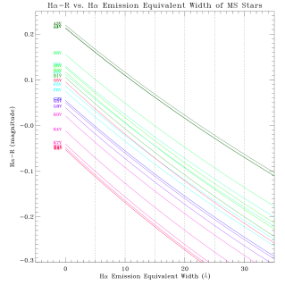
Figure 5.— H$\alpha-$R as a function of the H$\alpha$ emission equivalent width of main sequence stars for the Mosaic H$\alpha$ and R filters. (See electronic ApJ for the colored version.)

8. Chandra Optical Counterparts

8.1. X-ray source position error

Serendipitous X-ray sources in the ChaMPlane fields are detected from the Chandra archival data, using the methods (the ChaMPlane X-ray processing routines XPIPE and PXP) described in Hong et al. (2005). Each Chandra source has a position error that depends on the net source counts and off-axis angle from the aimpoint. The 95% confidence error radii, $r_{x(95\%)}$, are calculated as a function of net counts and off-axis angle, according to an empirical formula based on the results of raytrace simulations and XPIPE detections (Hong et al., 2005).

8.2. X-ray source boresight correction

Other than individual random errors, the Chandra sources also have a small systematic position offset, usually less than 1″ relative to the optical positions. Before matching X-ray and optical sources, the X-ray positions are corrected for this boresight difference ($\Delta\alpha$, $\Delta\delta$) that is determined for each observation separately.

To compute the boresight correction we first select Chandra sources with well-determined positions, i.e. $r_{x(95\%)}$ smaller than typically $1\arcsec$ to $2\arcsec$. If in the end it turns out that the final boresight is based on only a few (2 or 3) pairs of X-ray/optical matches, the limit on $r_{x(95\%)}$ is increased. Optical sources are selected from the Optical Catalog to have $R<23$ to guarantee good positions. If no $R$ magnitude is available, we require that the source is brighter than 23 in either $V$, $I$ or $H\alpha$ – in that order of priority.

The resulting X-ray and optical source lists are cross-correlated. Initially we accept matches inside a large match radius which combines statistical and systematic errors for a combined 2$\sigma$ value:

$$R_{0}=2\times\sqrt{r_{x}^{2}+r_{opt}^{2}+r_{xsys}^{2}}$$ (12)

where
$r_{x}=r_{x(95\%)}/1.95996$, is the 1-$\sigma$ random error on X-ray positions, assuming the errors follow a Gaussian distribution;
$r_{opt}=0.1\arcsec$ is the random error of individual optical positions with respect to the astrometric frame (see section 6); and
$r_{xsys}=0.6\arcsec/1.6449$, is the 1-$\sigma$ typical boresight offset of X-ray positions ($0.6\arcsec$ is the 90% absolute accuracy on Chandra positions).

A weighted (by 1/$r_{x(95\%)}$²) average offset in RA ($\Delta\alpha$) and Dec ($\Delta\delta$) (defined as the X-ray position minus the optical position) is computed after excluding X-ray sources with more than one possible (i.e. within $R_{0}$) optical counterpart. Errors on the offsets, $\Delta\alpha_{err}$ and $\Delta\delta_{err}$, are computed as the square-root of the weighted variance in $\Delta\alpha$ and $\Delta\delta$ divided by the number of matches. X-ray/optical matches whose individual offsets lie more than 3 $\times$ $\Delta\alpha_{err}$ or 3 $\times$ $\Delta\delta_{err}$ from the average are rejected, and the weighted average is re-computed.

After correcting the X-ray positions for $\Delta\alpha$ and $\Delta\delta$, the cross-correlation is repeated. In the second and consecutive iterations the match-radius is set as follows:

$$R_{1}=2\times\sqrt{r_{x}^{2}+r_{opt}^{2}+r_{bore}^{2}}$$ (13)

where $r_{bore}$ is the greater of $\Delta\alpha_{err}$ or $\Delta\delta_{err}$ in the previous iteration.

The above steps are iterated until the boresight correction converges to a stable solution, which is reached in typically 2 to 4 passes. The result is inspected visually against a Mosaic image; optical sources with positions that look unreliable (e.g. the position could be off from the center-of-light, or there could be a nearby undetected source) are removed from the catalog and the calculation is redone. The final stable solution of the boresight correction is applied to all the X-ray positions. As an example, the boresight solution for the GRO J0422+32 field is $\Delta\alpha=0.21\arcsec\pm 0.059\arcsec$ and $\Delta\delta=-0.36\arcsec\pm 0.044\arcsec$.

8.3. Optical Counterparts

The Optical Counterparts are found around the boresight corrected X-ray positions within an error radius of:

$$R_{err}=c\times\sqrt{r_{x}^{2}+r_{opt}^{2}+r_{bore}^{2}}$$ (14)

where $r_{x}$ and $r_{opt}$ are defined in Equation 12; $r_{bore}$ is the greater of $\Delta\alpha_{err}$ or $\Delta\delta_{err}$ in the final stable boresight solution; the square root expression is the combined effective matching error, $\sigma$; $c$ is a confidence-level scale factor (number of $\sigma$), and typically we choose $c=3$ to search for optical counterparts. For each Chandra source, we search the Mosaic optical catalog (see Section 5) within $R_{err}$ radius for its optical counterparts. If there are more than one matches within the $R_{err}$ radius, they are prioritized (for follow-up spectroscopy) by the matching distance and their H$\alpha-$R color. This process produces the Chandra optical counterparts from the Mosaic optical catalogs, which contain all the objects with magnitude ranging from $\sim$12 to $\sim$25. Thus it misses out stars brighter than $\sim$12 magnitude, which are saturated even in the short Mosaic images. To recover those possible missing bright star counterparts, we match all the Chandra sources, using the $R_{err}$ radii, with the USNO-A2 and GSC2 catalogs (see Section 3.2). This process produces all the Chandra optical counterparts with magnitude brighter than $\sim$19. When combining the results from these two matches, and removing the duplications (i.e. objects appear in both matches), we obtain a complete set of Chandra optical counterparts for a given field.

9. Results

9.1. ChaMPlane Optical Survey Products

The end products of the ChaMPlane optical photometry for each Mosaic field are:

1. An optical catalog of all the objects (regardless of object type e.g., stars, CV candidates, QSOs or galaxies, as determined by followup spectroscopy) detected in the entire Mosaic field. Each entry includes the source ID, RA and Dec, X and Y position on the image, V, R, I and H$\alpha$ magnitudes and their errors, as well as the PSF fitting parameters $\chi^{2}$ and sharpness, colors V$-$R, R$-$I, H$\alpha-$R and their errors, and S/N of H$\alpha-$R (as defined in Section 7).

2. A list of H$\alpha$ emission sources (as defined in Section 7) found in the entire Mosaic field.

3. A list or lists of Chandra optical counterparts (as defined in Section 8) found for every Chandra observation covered by this Mosaic field.

9.2. Example Results for GRO J0422+32 Field

In this section, we use the black hole X-ray nova GRO J0422+32 Chandra field (ObsID 676, 20 ks ACIS-I observation) as an example to demonstrate the typical output of the photometry survey. The optical catalog from this Mosaic field has 29714 entries, with magnitudes ranging from 12.4 to 25.5. The catalog is accessible at the ChaMPlane website${}^{\ref{cplweb}}$.

Table 3GRO J0422+32 field: H$\alpha$ emission sources within the Full Mosaic field

OptID	RA(J2000)	Dec(J2000)	V(err)	R(err)	I(err)	H$\alpha-$R	S/N	N
187498	04 20 17.07	$+$32 47 20.8	21.23(02)	20.21(01)	18.86(01)	$-$0.34(02)	18.92	1
108811	04 21 30.28	$+$33 07 29.2	21.05(01)	20.28(01)	19.79(02)	$-$0.76(01)	41.77	2
97731	04 21 42.72	$+$32 54 27.1	21.87(02)	20.80(01)	19.84(02)	$-$1.45(01)	61.43	3
99419	04 21 40.58	$+$33 12 04.1	21.71(02)	21.14(01)	20.77(05)	$-$0.45(02)	19.18	4
37863	04 22 43.56	$+$33 13 32.3	$-$	21.28(03)	19.55(03)	$-$0.35(04)	8.30	5
226061	04 19 53.04	$+$33 08 28.0	$-$	21.60(03)	20.77(08)	$-$0.42(04)	8.56	6
170813	04 20 33.62	$+$32 39 48.8	$-$	21.91(03)	20.19(03)	$-$0.32(04)	6.58	7
81814	04 22 00.25	$+$32 57 08.0	23.34(07)	21.98(03)	21.42(08)	$-$0.32(04)	6.44	8
130822	04 21 11.70	$+$32 38 38.4	22.98(07)	22.18(03)	21.46(09)	$-$0.55(05)	8.71	9
133739	04 21 08.55	$+$33 08 10.4	23.16(09)	22.22(04)	21.31(07)	$-$0.36(06)	5.43	10
165944	04 20 37.67	$+$33 09 57.1	23.16(07)	22.36(03)	21.68(09)	$-$0.43(05)	6.75	11
197374	04 20 07.98	$+$32 44 28.8	23.17(08)	22.43(04)	$-$	$-$1.04(05)	14.71	12
155336	04 20 48.59	$+$32 45 22.0	23.21(09)	22.68(04)	22.20(16)	$-$0.97(06)	11.36	13
133393	04 21 09.44	$+$32 40 59.9	23.57(13)	22.81(06)	$-$	$-$0.87(07)	8.29	14
87347	04 21 54.25	$+$32 47 35.2	24.51(24)	23.21(07)	$-$	$-$1.54(08)	10.20	15
81911	04 22 00.32	$+$32 42 16.6	24.11(16)	23.22(07)	22.62(23)	$-$0.76(10)	5.40	16
156015	04 20 47.83	$+$32 50 55.6	$-$	23.29(08)	22.77(25)	$-$0.89(10)	6.22	17
151985	04 20 51.72	$+$32 45 17.5	24.05(20)	23.63(10)	$-$	$-$1.80(11)	8.11	18

 R                   H$\alpha$

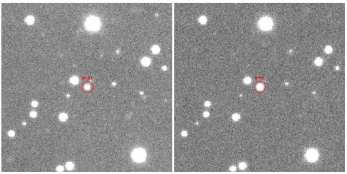
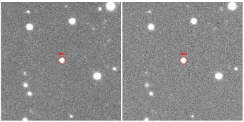
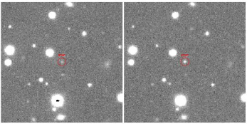
Figure 6.— The R (left) and H$\alpha$ (right) images of three H$\alpha$ emission sources found in the J0422+32 Mosaic field: 1) top panels show the GRO J0422+32 itself (circled), which is obviously brighter in H$\alpha$ (ID=97731, R = 20.80, H$\alpha-$R = $-$1.45); 2) middle panels show the first CV discovered under ChaMPlane project, which is outside of the ACIS FoV (ID=108811, R = 20.28, H$\alpha-$R = $-$0.76); 3) bottom panels show a very bright H$\alpha$ emission object (ID=87347, R = 21.67, H$\alpha-$R = $-$1.54). It is in the ACIS-I FoV. Although no X-ray emission was detected from this object, the upper limit for $F_{x}/F_{r}$ allows it to be a CV. ($1\arcmin\times 1\arcmin$ FoV.)

Table 3 is a list of H$\alpha$ emission sources with H$\alpha-$R$\leqslant$$-$0.3 and S/N$\geqslant$5 (these criteria can, of course, be changed to select different H$\alpha$ sources). There are 18 H$\alpha$ sources that satisfy these criteria. Among them, ID 97731 is J0422+32 itself. It has very strong H$\alpha$ emission (H$\alpha-$R = $-$1.45 and S/N = 61.4) and therefore it was easily detected in our survey. ID 108811 is the first CV discovered under the ChaMPlane project. It has strong H$\alpha$ emission (H$\alpha-$R = $-$0.76 and S/N = 41.8). It was found outside the ACIS FoV so we do not know its X-ray properties. Its CV status was confirmed via spectroscopy (Rogel et al., 2005). ID 87347 is a very strong H$\alpha$ emission object with H$\alpha-$R = $-$1.54 and S/N = 10.2, corresponding to EW = 320Å based on Figure 4. It is also (barely) detected in B images taken with the Wide Field Camera on the 2.5-m Isaac Newton Telescope on La Palma, on Jan 13, 2004. A preliminary estimate gives B=25.1(2). This object is inside the ACIS-I FoV. However, no X-ray emission was detected from this object. The (unabsorbed) flux detection limits (3-$\sigma$) of this object are $uFx(0.5-2.0keV)\leqslant 2.5\times 10^{-15}ergs\,cm^{-2}sec^{-1}$, $uFx(2.0-8.0keV)\leqslant 9.5\times 10^{-15}ergs\,cm^{-2}sec^{-1}$, and $uFx(0.5-8.0keV)\leqslant 5.6\times 10^{-15}ergs\,cm^{-2}sec^{-1}$, assuming N${}_{\rm H}=1.9\times 10^{21}$, based on Schlegel et al. (1998), and a power-law spectrum with $\Gamma=1.7$. This yields the absorbed and unabsorbed flux ratios $F_{x}(Hc)/F_{r}\leqslant 10.4$ and $uF_{x}(Hc)/uF_{r}\leqslant 5.2$. This object can potentially be a CV, because its EW is much too large to be a dMe star. Deeper Chandra images and optical spectra are required, though this shows the generally comparable depths of the Mosaic and Chandra-ChaMPlane images. Figure 6 shows the R and H$\alpha$ images of these three H$\alpha$ emission sources.

Table 4 is a list of point Mosaic optical sources (i.e. $|sharpness|<1$) found within the match-radii (Eq. 14) of all the level 2 Chandra sources. XPIPE detected 62 point sources on the four ACIS-I chips. One of the 62 is the target – J0422. The other 61 are all newly discovered X-ray sources, based on a search in the SIMBAD Astronomical Database. 37 of these X-ray sources match with 43 point optical counterparts within the 3-$\sigma$ search radius. Four of the X-ray sources have two possible counterparts each and one X-ray source has three possible counterparts within the 3-$\sigma$ error circle.

Table 4GRO J0422+32 field: Chandra Optical Counterparts (point sources)

SrcID	OptID	RA(J2000)	Dec(J2000)	$r$	$d$	$\sigma$	$F_{x}$	$F_{x}/F_{r}$	$F_{x}/F_{r}$	V(err)	R(err)	I(err)	H$\alpha-$R	S/N
				(″)	(″)	($\sigma$)	(Bc)	(Sc)	(Hc)	(mag)	(mag)	(mag)	(mag)
B0_001	80714	04 22 01.58	$+$32 57 29.3	0.94	0.20	0.63	43.94	2.915	5.351	21.88(02)	21.53(02)	20.72(04)	0.17(04)	4.44
B0_002	82718	04 21 59.17	$+$32 57 58.4	1.25	0.36	0.86	15.81	4.050	12.988	24.00(17)	23.20(07)	22.33(18)	$-$0.04(14)	0.28
B0_003	89269	04 21 51.97	$+$32 57 06.8	0.90	0.29	0.97	14.62	3.651	10.253	23.69(11)	23.12(06)	22.28(15)	0.24(14)	1.54
B0_004	92541	04 21 48.36	$+$32 58 15.9	1.25	0.05	0.13	11.53	1.017	0.996	22.24(03)	21.69(02)	21.10(05)	0.07(04)	1.95
B0_005	81814	04 22 00.25	$+$32 57 08.0	3.06	1.15	1.13	2.71	0.296	0.402	23.34(07)	21.98(03)	21.42(08)	$-$0.32(04)	6.44
B0_007	94647	04 21 45.99	$+$32 58 45.3	1.46	0.21	0.44	7.27	0.854	3.196	23.09(07)	22.42(04)	21.81(10)	0.09(07)	1.19
B0_008	95706	04 21 44.84	$+$33 00 29.2	1.52	0.35	0.70	22.68	2.692	9.002	23.03(07)	22.38(03)	21.88(12)	0.14(07)	1.86
B0_009	70708	04 22 12.67	$+$33 01 26.9	5.53	0.12	0.06	13.25	0.678	0.820	21.64(02)	21.13(01)	20.67(04)	0.00(02)	0.00
B0_010	75612	04 22 07.22	$+$32 57 07.0	4.29	3.21	2.25	5.51	0.003	0.133	19.26(01)	18.48(00)	17.80(01)	0.00(01)	0.42
B0_010	75913	04 22 06.87	$+$32 57 06.2	4.29	1.56	1.09	5.51	0.046	2.372	22.83(06)	21.60(02)	20.67(04)	$-$0.01(04)	0.28
B0_014	85213	04 21 56.39	$+$33 03 39.0	3.47	1.44	1.24	22.22	3.041	5.763	22.92(07)	22.32(03)	22.18(15)	0.11(07)	1.52
B0_015	86506	04 21 55.04	$+$33 00 36.3	2.94	0.24	0.24	9.08	0.201	1.471	21.47(02)	20.99(01)	20.68(04)	0.08(03)	3.17
B0_017	72773	04 22 10.35	$+$33 01 26.0	5.78	0.54	0.28	7.82	0.454	0.130	21.49(02)	21.09(01)	20.61(04)	0.03(03)	1.04
B0_018	98282	04 21 42.03	$+$33 02 22.1	6.77	6.17	2.73	9.05	1.276	7.202	$-$	22.83(06)	22.28(18)	$-$0.04(11)	0.31
B0_018	98409	04 21 41.87	$+$33 02 23.0	6.77	4.44	1.97	9.05	0.059	0.333	20.67(01)	19.49(01)	18.35(01)	$-$0.12(01)	11.63
B0_018	98682	04 21 41.59	$+$33 02 25.8	6.77	2.13	0.94	9.05	1.522	8.595	23.57(10)	23.02(07)	$-$	0.19(15)	1.19
B1_001	87169	04 21 54.39	$+$32 53 09.8	1.07	0.27	0.75	7.75	0.601	0.482	22.07(03)	21.52(02)	21.16(06)	0.06(03)	1.66
B1_002	81268	04 22 00.97	$+$32 52 36.4	1.04	0.25	0.73	21.83	0.976	0.629	21.35(02)	20.89(01)	20.35(03)	$-$0.01(02)	0.72
B1_004	92607	04 21 48.36	$+$32 54 04.2	1.12	0.20	0.54	2.51	0.120	1.602	$-$	22.27(03)	21.29(08)	0.17(07)	2.03
B1_006	71512	04 22 11.83	$+$32 56 04.3	1.42	0.53	1.12	31.82	0.555	2.120	20.76(01)	20.36(01)	19.70(02)	0.12(02)	5.22
B2_003	110429	04 21 28.65	$+$32 55 46.9	1.14	0.24	0.64	8.04	2.817	$-$	23.71(12)	22.96(06)	21.96(13)	0.10(12)	0.76
B2_004	111561	04 21 27.42	$+$32 55 51.5	1.64	0.60	1.09	4.63	2.067	1.541	$-$	23.41(09)	22.32(17)	0.04(18)	0.23
B2_008	123049	04 21 17.27	$+$33 00 31.1	3.23	0.73	0.68	21.28	1.340	4.630	22.20(04)	21.70(03)	$-$	0.14(05)	2.51
B2_008	123477	04 21 17.01	$+$33 00 31.4	3.23	2.57	2.39	21.28	0.412	1.422	21.67(02)	20.42(01)	19.14(01)	$-$0.08(02)	4.64
B2_011	122729	04 21 17.47	$+$33 02 05.6	8.02	0.57	0.21	11.56	0.031	0.448	19.64(01)	19.20(01)	18.53(01)	0.07(01)	6.40
B2_012	115387	04 21 23.27	$+$33 02 12.6	9.57	3.51	1.10	7.75	0.112	0.371	21.11(01)	20.08(01)	19.26(01)	$-$0.06(01)	5.29
B2_013	133097	04 21 09.40	$+$32 55 42.3	8.46	2.09	0.74	6.80	0.543	13.065	$-$	23.32(09)	21.70(12)	0.23(20)	1.05
B3_001	95243	04 21 45.50	$+$32 51 58.9	0.84	0.17	0.59	16.14	5.790	15.310	24.08(16)	23.49(10)	22.66(26)	0.03(21)	0.14
B3_003	97731	04 21 42.72	$+$32 54 27.1	0.70	0.10	0.43	10.15	0.422	0.249	21.87(02)	20.80(01)	19.84(02)	$-$1.45(01)	61.43
B3_005	106618	04 21 32.88	$+$32 53 27.3	0.91	0.16	0.52	9.81	0.013	0.004	18.35(00)	17.00(01)	15.54(00)	$-$0.19(01)	24.40
B3_006	95130	04 21 45.62	$+$32 51 14.6	0.88	0.16	0.54	25.04	2.462	13.008	$-$	22.42(04)	22.01(15)	0.06(07)	0.95
B3_008	111135	04 21 27.94	$+$32 53 02.1	1.33	0.46	1.03	10.74	0.014	0.009	18.53(01)	17.08(01)	15.42(01)	$-$0.20(01)	15.82
B3_009	111329	04 21 27.76	$+$32 50 38.3	1.45	0.48	0.99	15.59	1.706	2.669	22.89(05)	22.04(02)	21.59(08)	$-$0.26(04)	5.26
B3_010	112331	04 21 26.61	$+$32 51 34.8	2.38	0.75	0.95	4.45	0.002	0.001	16.52(01)	15.94(01)	15.37(01)	$-$0.04(01)	3.90
B3_011	86630	04 21 55.08	$+$32 47 26.0	1.75	0.89	1.52	45.50	1.527	4.094	21.57(02)	20.93(01)	20.22(03)	$-$0.01(02)	0.49
B3_012	88797	04 21 52.60	$+$32 47 01.0	7.24	6.12	2.53	6.27	0.057	0.029	19.91(01)	19.15(01)	18.45(01)	0.02(01)	1.55
B3_012	89291	04 21 52.09	$+$32 47 04.1	7.24	1.15	0.48	6.27	2.300	1.172	$-$	23.16(07)	22.57(22)	0.23(17)	1.23
B3_013	90634	04 21 50.62	$+$32 47 55.1	9.63	7.25	2.26	1.18	0.041	0.297	22.40(04)	21.49(02)	20.71(04)	$-$0.11(03)	3.22
B3_015	99529	04 21 40.82	$+$32 49 40.5	2.77	1.13	1.22	6.62	0.409	7.764	23.31(09)	22.85(05)	$-$	$-$	0.00
B3_018	115085	04 21 23.78	$+$32 48 37.8	1.60	0.65	1.22	43.27	2.681	6.901	22.18(03)	21.58(02)	21.08(05)	$-$0.01(04)	0.28
B3_019	120062	04 21 19.83	$+$32 49 02.6	3.15	1.14	1.08	16.01	0.014	0.005	17.78(01)	16.56(01)	15.45(01)	$-$0.11(01)	7.33
B3_021	120888	04 21 19.25	$+$32 47 49.6	7.30	7.22	2.97	7.26	2.374	6.582	$-$	23.41(10)	$-$	$-$0.02(23)	0.08
B3_021	121522	04 21 18.81	$+$32 47 48.2	7.30	1.63	0.67	7.26	0.594	1.647	22.50(06)	21.91(03)	$-$	0.03(05)	0.61

Table 5 is a list of extended optical counterparts (i.e. $sharpness\geqslant 1$) of Chandra sources from the Mosaic catalog. There are 3 X-ray sources which match with 3 extended optical counterparts. They are most likely galaxies.

A search of USNO-A2 and GSC2 catalogs yields 6 and 5 optical counterparts, respectively. However, all of them are duplicates, i.e. they are already included in the list of the Mosaic optical counterparts. Therefore, by combining Table 4 and Table 5, there are 40 Chandra sources matching with 46 (point or extended) optical counterparts, which is the complete set of Chandra optical counterparts in the J0422+32 field.

Table 5GRO J0422+32 field: Chandra Optical Counterparts (extended sources)

SrcID	OptID	RA(J2000)	Dec(J2000)	$r$	$d$	$\sigma$	$F_{x}$	$F_{x}/F_{r}$	$F_{x}/F_{r}$	V(err)	R(err)	I(err)	H$\alpha-$R	S/N
				(″)	(″)	($\sigma$)	(Bc)	(Sc)	(Hc)	(mag)	(mag)	(mag)	(mag)
B1_005	71306	04 22 12.08	$+$32 53 57.4	2.45	0.36	0.45	10.01	$-$	$-$	19.14(04)	$-$	17.38(04)	$-$	0.00
B1_009	81365	04 22 00.85	$+$32 51 04.0	3.29	0.95	0.86	7.29	0.382	1.013	22.71(06)	21.41(03)	20.31(04)	0.05(05)	1.01
B2_001	105760	04 21 33.83	$+$32 55 57.4	0.70	0.32	1.36	31.96	1.018	4.109	21.88(05)	21.05(06)	20.08(05)	0.18(09)	1.89

See footnotes of Table 4 for column definitions.

Table 6 is a list of 22 Chandra sources without optical counterparts, with their optical magnitude limit as measured with the Mosaic photometry.

Table 6GRO J0422+32 field: Chandra Sources without Optical Counterparts

						Magnitude limits
SrcID	RA(J2000)	Dec(J2000)	$F_{x}$	$F_{x}$	$F_{x}$	V	R	I	H
			(Bc)	(Sc)	(Hc)	(mag)	(mag)	(mag)	(mag)
B0_006	04 21 49.07	$+$32 58 46.1	4.68	1.07	3.53	24.80	24.70	22.90	24.30
B0_011	04 21 59.30	$+$33 01 01.2	10.32	2.11	9.03	24.71	24.96	22.86	24.44
B0_012	04 21 59.34	$+$33 00 21.3	4.36	1.67	0.10	24.63	25.03	23.01	24.29
B0_013	04 21 56.36	$+$33 03 05.7	13.30	1.20	18.96	24.61	24.63	22.97	24.22
B0_016	04 21 40.52	$+$33 03 08.3	14.47	2.39	15.51	24.69	24.96	22.98	24.16
B1_003	04 21 52.74	$+$32 53 45.5	7.59	2.27	3.12	24.48	24.28	22.99	24.08
B1_007	04 22 01.71	$+$32 51 57.5	3.94	1.04	2.25	24.65	24.85	23.00	24.33
B1_008	04 22 13.56	$+$32 51 45.4	6.29	1.24	5.65	24.55	24.93	22.94	24.13
B2_002	04 21 40.39	$+$32 55 57.9	6.50	0.98	7.28	24.69	24.72	22.88	24.30
B2_005	04 21 38.25	$+$32 58 40.2	9.76	2.31	7.03	24.82	24.78	22.78	24.38
B2_006	04 21 28.75	$+$32 56 58.2	4.01	$-$	7.53	24.72	24.66	22.84	24.30
B2_007	04 21 22.15	$+$33 01 07.0	11.22	0.89	16.66	24.58	25.01	22.87	24.16
B2_009	04 21 29.63	$+$33 01 10.8	18.15	4.71	11.26	24.76	24.97	22.96	24.43
B2_010	04 21 25.01	$+$32 59 43.0	4.14	0.48	5.43	24.89	24.95	22.87	24.18
B2_014	04 21 19.28	$+$32 58 07.2	7.03	2.19	2.58	24.55	24.67	22.90	24.22
B3_002	04 21 44.82	$+$32 54 04.1	7.67	1.73	5.85	24.70	24.94	22.84	24.44
B3_004	04 21 41.18	$+$32 53 13.5	14.85	3.97	8.29	24.59	24.90	22.99	24.16
B3_007	04 21 43.45	$+$32 49 44.7	8.79	2.10	6.03	24.58	25.03	23.10	24.33
B3_014	04 21 46.60	$+$32 52 40.4	1.92	0.50	1.14	24.67	24.73	22.85	24.20
B3_016	04 21 26.98	$+$32 48 58.9	5.06	1.45	2.31	24.61	24.88	23.04	24.09
B3_017	04 21 25.51	$+$32 52 28.8	2.90	1.15	$-$	24.76	24.84	22.97	24.40
B3_020	04 21 18.66	$+$32 52 55.6	6.19	1.79	2.79	24.65	24.73	22.91	24.25

Table 7 is a list of 5 bright stars in the Henry Draper (HD) Catalog, found within the ACIS-I FoV through a SIMBAD search, with their known spectral type and (for late-type stars only) expected X-ray flux ranges for late-type stars only based on ROSAT observations (Schmitt & Liefke, 2004). None of these 5 stars were detected by the Chandra observation of J0422. The soft band flux detection limit at position of these 5 stars are also listed in the Table.

Table 7J0422+32 field: Bright HD Stars within the ACIS-I FoV

ID	RA(J2000)	Dec(J2000)	B	V	Type	d	N${}_{\rm H}/10^{22}$	Expected $F_{x}$	$F_{x}$-lim	$uF_{x}$-lim
						(pc)	$cm^{-2}$	Min – Max	(Sc)	(Sc)
HD281972	04:21:12.70	$+$32:54:39.2	9.5	$-$	B9	748	0.189	–	1.63	2.59
HD281969	04:21:51.45	$+$32:53:34.2	11.7	11.0	A2	344	0.194	–	1.56	2.50
HD281970	04:21:46.14	$+$32:57:31.5	11.6	10.9	F2	183	0.188	0.08 – 134	2.11	3.34
HD281973	04:21:11.25	$+$32:49:48.8	10.07	9.55	F8	129	0.200	0.16 – 270	3.85	6.24
HD281971	04:21:19.78	$+$33:00:17.4	9.5	$-$	K0	36	0.174	2.12 – 789	2.82	4.33

Figure 7 shows the final stacked deep R image of the field GRO J0422+32, which consists of 10 individual (two sets of 5 dithered) images, with a total exposure time of 2100 seconds. It also shows the ACIS, Chandra sources and their optical counterparts and H$\alpha$ emission sources overlay. Figure 8 is the same figure but zoomed in around the ACIS-I aimpoint.

Figure 9 shows the J0422+32 field (H$\alpha-$R) vs. R color-magnitude and (V$-$R) vs. (R$-$I) color-color diagrams within the ACIS-I FoV. Figure 10 shows the same diagrams of objects outside the ACIS-I FoV.

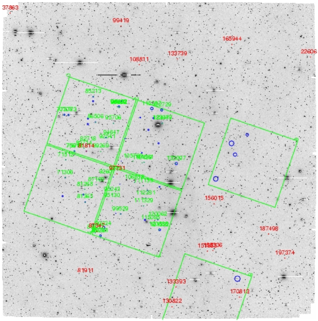
Figure 7.— GRO J0422+32 field full Mosaic deep R image with active ACIS CCDs overlay (large green squares, ACIS I0-3 and S2,4 were turned on). Chandra source 3-$\sigma$ error circles are marked with blue color. Chandra candidate optical counterparts are marked by small (1″) green circles with their optical ID. H$\alpha$ emission sources (H$\alpha-$R$\leqslant$$-0.3$ and S/N$\geqslant$5) are marked with (1.5″) red circles with their optical ID. ID 108811 (above the ACIS-I) is the first CV discovered under the ChaMPlane project. ID 87347 (near the bottom of ACIS-I) is the previously unknown bright H$\alpha$ emission object without X-ray detection. Five X-ray sources are detected on the ACIS-S2 and S4 chips. We do not include their optical counterparts here as their positional errors are relatively poorly known due to their large off-axis angles. (North-up, east-left; $36\arcmin\times 36\arcmin$ FoV.) (See electronic ApJ for the colored version.)

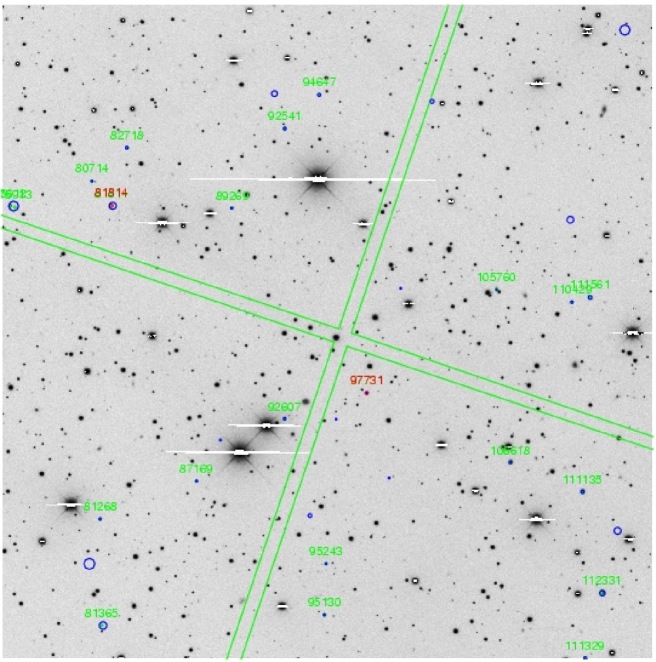
Figure 8.— GRO J0422+32 field Mosaic deep R image around the ACIS-I aimpoint (See Figure 7 for source marker notations). ID 97731 at the aimpoint is the target J0422+32. ID 81814 is the only other H$\alpha$ emission Chandra source on ACIS-I, which is a QSO at z=4.25, with Lyman-$\alpha$ red-shifted to Balmer-$\alpha$ (Rogel et al., 2005). (North-up, east-left. ($9\arcmin\times 9\arcmin$ FoV.) (See electronic ApJ for the colored version.)

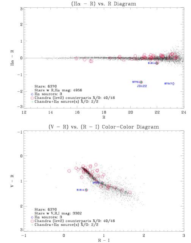
Figure 9.— GRO J0422+32 field (H$\alpha-$R) vs. R color-magnitude and (V$-$R) vs. (R$-$I) color-color diagrams of objects inside ACIS-I FoV. 40 Chandra sources are matched with 46 counterparts (marked as red circles). There are three H$\alpha$ emission sources (marked as blue diamonds) within the ACIS-I FoV. Two of them are Chandra sources: ID 97731 is the black-hole X-ray nova J0422+32 ; ID 81814 is a quasar at z=4.25. ID 87347 is an unclassified bright H$\alpha$ emission object without X-ray detection. (See electronic ApJ for the colored version.)

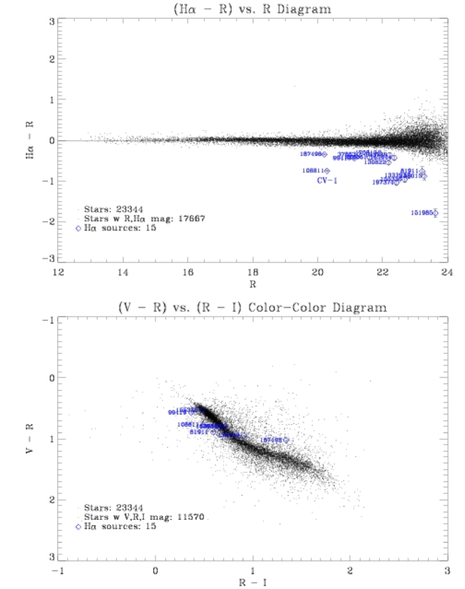
Figure 10.— GRO J0422+32 field (H$\alpha-$R) vs. R color-magnitude and (V$-$R) vs. (R$-$I) color-color diagrams of objects outside ACIS-I FoV. There are 15 H$\alpha$ emission sources. The object with ID 108811 is the first CV discovered under the ChaMPlane project. (See electronic ApJ for the colored version.)

9.3. Follow-up Observations

The next step of the ChaMPlane optical survey is to obtain the optical spectra of all the H$\alpha$ emission sources and the Chandra optical counterparts found in the ChaMPlane photometry in order to determine the nature of the objects. This is the final, crucial step for completing the survey. We have been conducting the spectroscopic follow-up using the WIYN 3.5-m (Rogel et al., 2005) and MMT 6.5-m telescopes for the northern ChaMPlane fields and the CTIO 4-m and Magellan 6.5-m telescopes for the southern fields. Because of the severe extinction in visible bands towards the Galactic center, we are also carrying out infrared imaging photometry for the Galactic bulge fields (Laycock et al., 2005).

10. Summary

We have successfully conducted and completed the optical imaging and Mosaic photometry for the ChaMPlane survey. Considerable followup work (spectroscopy as well as additional photometry analysis) is now in progress to identify the nature of the sources and will be reported in subsequent papers. The photometry survey obtained 65 Mosaic fields, or $\sim$23 square degrees in the Galactic plane and covers 154 Chandra observations on 105 distinct Chandra fields, which is what we proposed to accomplish. Using 6 Mosaic pointings, we mapped out 2.2 square degrees around the Galactic center using V, R, I and H$\alpha$ filters to cover 58 Chandra ACIS observations. This is the deepest optical survey towards the Galactic center, so far.

This paper summarizes our Mosaic photometry observations and describes our data reduction method. Deep Mosaic imaging produces comprehensive optical catalogs for each ChaMPlane field. The R and H$\alpha$ differential photometry efficiently detects H$\alpha$ emission sources. Our search method effectively finds the optical counterparts for the majority of Chandra sources in the low extinction fields. Spectroscopy follow-ups for the Chandra optical counterparts and H$\alpha$ emission sources for classification complete the ChaMPlane survey. All the optical catalogs produced by the ChaMPlane optical survey will be available at the ChaMPlane Online Database and NOAO Science Archive. This legacy Optical Database will provide a rich resource for Galactic astronomy.

References

- Grindlay et al. (2003) Grindlay, J.E. et al. 2003, Astronomische Nachrichten, V324, No.1-2, 57-60
- Grindlay et al. (2005) Grindlay, J.E. et al. 2005, ApJ, submitted
- Hong et al. (2005) Hong, J. et al. 2005, ApJ, submitted
- Landolt (1992) Landolt, A.U. 1992, ApJ, 104, 340
- Laycock et al. (2005) Laycock, S. et al. 2005, ApJ, submitted
- Mochnacki et al. (2002) Mochnacki, S. et al. 2002, AJ, 124, 2868
- Muno et al. (2003) Muno, M.P. et al. 2003, ApJ 589, 225
- Rogel et al. (2005) Rogel, A.B. et al. 2005, ApJ, submitted
- Schlegel et al. (1998) Schlegel, D., Finkbeiner, D., & Davis, M., ApJ, 1998, 500, 525
- Schmitt & Liefke (2004) Schmitt, J.H.M.M. & Liefke C. 2004, A&A 417, 651
- Szkody et al. (2002) Szkody, P. et al. 2002, AJ, 123, 430
- Szkody et al. (2003) Szkody, P. et al. 2003, AJ, 126, 1499
- Szkody et al. (2004) Szkody, P. et al. 2004, AJ, 128, 1882
- Szkody et al. (2005) Szkody, P. et al. 2005, AJ, 129, 2386
- Wang et al. (2002) Wang, D. et al. 2002, Nature, 415, 148
- Warner (1995) cf. Warner, B. “Cataclysmic variable stars”, Cambridge University Press, 1995
- William (1983) William, G. 1983, ApJS, 53, 523 148
- Zhao et al. (2003) Zhao, P. et al. 2003, Astronomische Nachrichten, V324, No.1-2, 176