X-ray Processing of ChaMPlane Fields:
Methods and Initial Results for Selected Anti-Galactic Center Fields

Abstract

We describe the X-ray analysis procedure of the on-going Chandra Multiwavelength Plane (ChaMPlane) survey and report the initial results from the analysis of 15 selected anti-Galactic center observations ($90\mbox{${}^{\circ}$}<l<270\mbox{${}^{\circ}$}$). We describe the X-ray analysis procedures for ChaMPlane using custom-developed analysis tools appropriate for Galactic sources but also of general use: optimum photometry in crowded fields using advanced techniques for overlapping sources, rigorous astrometry and 95% error circles for combining X-ray images or matching to optical/IR images, and application of quantile analysis for spectral analysis of faint sources. We apply these techniques to 15 anti-Galactic center observations (of 14 distinct fields) in which we have detected 921 X-ray point sources. We present log$N$-log$S$ distributions and quantile analysis to show that in the hard band (2 – 8 keV) active galactic nuclei dominate the sources. Complete analysis of all ChaMPlane anti-Galactic center fields will be given in a subsequent paper, followed by papers on sources in the Galactic center and Bulge regions.

1. Introduction

The on-going Chandra Multiwavelength Plane (ChaMPlane) survey is designed to constrain the low-luminosity accretion source content and stellar-coronal source luminosity functions in the Galaxy (Grindlay et al., 2003, 2005). To achieve this goal we search for low-luminosity Galactic X-ray sources in Chandra archival data and attempt to identify them using follow-up optical and/or infrared (IR) imaging and spectroscopic observations.

This paper describes the X-ray analysis of the ChaMPlane survey. To illustrate the procedures, we describe the initial X-ray results from the analysis of 15 selected anti-Galactic center (anti-GC) observations ($90\mbox{${}^{\circ}$}<l<270\mbox{${}^{\circ}$}$; Table 1). §2 describes the custom analysis tools developed for the project. §3 presents initial results including log$N$-log$S$ distributions of the sources and basic source properties using a new X-ray spectral classification technique – quantile analysis (Hong et al., 2004).

In subsequent papers, we will present the X-ray results of all anti-GC fields and the Galactic-Bulge and Center region sources. The overview of the project is given in Grindlay et al. (2005). The methodology and initial results of the optical and IR surveys are presented in Zhao et al. (2005), Rogel et al. (2005) and Laycock et al. (2005), respectively.

Table 115 selected ChaMPlane observations in the anti-GC region (sorted by Galactic longitude except for the stacked data)

		$l$	$b$	Exposurea	$N_{\mbox{\scriptsize H}}$b	No. of		Obs. Date	CCDs										Aimd
Obs. ID	Target	(deg)	(deg)	(ksec)	($\mbox{$\times$}10^{22}$cm-2)	Sourcesc		(y-m-d)	used										ACIS-
2787	PSR J2229+6114	106.64900	2.94848	91.5	1.04 / 0.40	91		02-03-15	0	1	2	3	.	.	6	7	.	.	I
1948	3EG J2227+6122	106.64901	2.94965	14.7	1.02 / 0.40	20		01-02-14	0	1	2	3	.	.	6	7	.	.	I
755	B2224+65	108.63800	6.84522	47.6	0.44 / 0.23	78		00-10-21	.	.	2	3	.	5	6	7	8	.	S
2810	G116.9+0.2	116.94330	0.18420	48.8	0.48 / 0.28	97		02-09-14	0	1	2	3	.	.	6	7	.	.	I
2802	G127.1+0.5	127.11343	0.53889	19.2	0.89 / 0.31	44		02-09-14	0	1	2	3	.	.	6	7	.	.	I
782	NGC1569	143.68323	11.24151	93.3	0.42 / 0.11	89		00-04-11	0	1	2	3	.	5	.	7	.	.	S
650	GK Persei	150.95713	$-$10.10413	90.3	0.20 / 0.10	83		00-02-10	.	.	2	3	.	5	6	7	8	.	S
2218	3C 129	160.42891	0.13717	30.2	0.63 / 0.24	25		00-12-09	.	.	.	.	4	5	6	7	8	9	S
676	GRO J0422+32	165.88229	$-$11.91286	18.7	0.19 / 0.09	67		00-12-09	0	1	2	3	.	.	6	.	8	.	I
2803	G166.0+4.2	166.13140	4.33778	29.3	0.38 / 0.19	53		02-01-30	0	1	2	3	.	.	6	7	.	.	I
829	3C 123	170.58315	$-$11.66140	46.3	0.59 / 0.12	52		00-03-21	.	.	2	3	.	5	6	7	8	.	S
2796	PSR J0538+2817	179.71974	$-$1.68585	19.4	0.80 / 0.26	31		02-02-07	.	.	2	3	.	5	6	7	8	.	S
95	A0620$-$00	209.95777	$-$6.54014	41.2	0.29 / 0.18	61		00-02-29	.	.	.	3	.	5	6	7	8	.	S
2553	Maddalena’s Cloud	216.73098	$-$2.60034	24.5	0.93 / 0.27	59		02-02-08	0	1	2	3	.	.	6	7	.	.	I
2545	M1$-$16	226.80033	5.62592	48.6	0.13 / 0.12	71		02-02-11	.	.	2	3	.	5	6	7	8	.	S
e52787	2787 & 1948 Stacked	106.64900	2.94848	106.2	1.04 / 0.40	90		–	0	1	2	3	.	.	.	.	.	.	I

^aSum of the good time intervals (GTIs, §2.1).
^bTwo estimates; Schlegel et al. (1998) / Drimmel et al. (2003). The total sum along the line of the sight, averaged over source positions. See §2.2.2 for the differences in the two models.
^cNumber of valid (level 1) sources found in the $B_{X}$ band. See Tables 2 and 4 for the definition of bands and levels.
^dAim point detector: I = CCD 3 and S = CCD 7.
^eThe combined data (CCD 0, 1, 2, 3) of two stackable observations (1948 and 2787). See §2.1 and Table 3.

2. Data Analysis

The overall data analysis procedures can be grouped into two stages. First, we search for X-ray point sources using a wavelet detection algorithm (wavdetect; Mallat, S. 1998; Freeman et al. 2002; §2.1). Second, we determine various source properties using simple aperture photometry (§2.2). To apply the above algorithms consistently on the large ChaMPlane data set, we employed a custom X-ray analysis tool (XPIPE) and have developed post-XPIPE procedures (PXP). Both tools are primarily based on CIAO tools (version 3.1).

XPIPE is an X-ray analysis tool developed for the Chandra Multiwavelength Project (ChaMP) which is a high-latitude extra-Galactic survey for active galactic nuclei (AGN) (Kim et al. 2004a and 2004b; K04 hereafter). The scientific goals of the two projects, ChaMP and ChaMPlane, are as different as the survey regions – Galactic Plane survey versus high-latitude survey. However, both projects share similar requirements for the analysis, namely, searching for faint X-ray point sources in Chandra ACIS archival data. This analysis similarity and the success of XPIPE in the ChaMP analysis (K04) led us to adopt XPIPE as our primary tool. The detailed description of XPIPE can be found in K04, and in what follows we only briefly review the basics that are relevant for ChaMPlane.

In addition to XPIPE and in order to meet ChaMPlane-specific analysis requirements, we have also developed our own analysis tool, PXP, which is described below. PXP uses XPIPE outputs and performs analysis that is optimized for Galactic sources but also of general use.

2.1. Source detection by wavdetect

For each observation, we start the analysis by using XPIPE on the level 2 data products generated by the Chandra X-ray Center (CXC) standard data processing. First, XPIPE removes the residual artifacts that may be present after the CXC standard data processing. XPIPE then selects events in the good time intervals (GTIs) which are selected to have fluctuations $<3\sigma$ from the mean background rate.

Table 2Energy bands for the ChaMPlane X-ray analysis

Type		Name	Range
XPIPE wavdetect band
	Soft	$S_{X}$	0.3 – 2.5 keV
	Hard	$H_{X}$	2.5 – 8.0 keV
	Broad	$B_{X}$	0.3 – 8.0 keV
Conventional band
	Soft	$S_{C}$	0.5 – 2.0 keV
	Hard	$H_{C}$	2.0 – 8.0 keV
	Broad	$B_{C}$	0.5 – 8.0 keV

For source detection, XPIPE uses wavdetect with a significance threshold of $10^{-6}$ (about 1 possibly spurious detection per CCD, see K04 for the detailed analysis of source detection efficiency with wavdetect in XPIPE) and a scale parameter varying in seven steps between 1 and 64 pixels to cover a wide range of source sizes. XPIPE applies wavdetect in three separate energy bands, $S_{X}$, $H_{X}$ and $B_{X}$ (Table 2), using the exposure map generated at 1.5 keV. Note that the wavdetect routine in CIAO version 3.1 includes source position refinement procedures that had to be applied separately in the old version of XPIPE based on CIAO version 2.3 (K04).

When multiple observations of a similar region of the sky are available, it is possible to combine the data sets to look for fainter sources and to study variability. Particularly near or at the GC region, many stackable observations are available (Grindlay et al., 2005). We have devised PXP so that it can employ wavdetect on stacked images. We consider multiple observations stackable if their aimpoints are within 1^′ of each other and the aimpoint detectors are the same type (ACIS-I or ACIS-S). Among the stackable observations, we designate the one with the longest exposure to be the base observation of the stacked image. For the analysis convenience, we assign a separate Obs. ID for the stacked data ($xyyyy$, where $x$ is $>5$ and $yyyy$ is the base Obs. ID) and we assign the CCD ID of the stacked data to be 3 for ACIS-I and 7 for ACIS-S observations. For stacking, we only use the data of CCD 0, 1, 2, 3 for ACIS-I and the data of CCD 7 for ACIS-S observations. For the aimpoint, detector response function, and other required parameters of the stacked data, we employ the same of the base observation. In the anti-GC fields (Table 1), Obs. ID 52787 is the stacked data of two observations (1948 and 2787) and Obs. ID 2787 is the base observation of the two.

Before we stack the data, we apply astrometric corrections (see also §2.3). First, we calculate the correction for the aspect offset of each observation. Second, we calculate the boresight offset of each observation relative to the base observation using the aspect-corrected position of the wavdetected sources. The final boresight offset of each observation is derived by an iterative procedure using a relatively more reliable subset of matching source pairs. The iterative technique is identical to the boresight correction procedure employed between X-ray and optical data for the optical ChaMPlane survey (Zhao et al., 2005) except that the procedure is applied between X-ray and X-ray data using the estimated 95% X-ray positional errors (§2.3).

For the purpose of stacking the X-ray data pointed to a similar region of the sky (i.e. large overlap in the field of view), direct comparison of the boresight of an X-ray observation to another X-ray observation is more efficient than comparing it to observations (or catalogs) in another wavelength because the number of matching pairs found in the former case is likely larger than that in the latter and a large number of matching pairs usually provide a reliable estimation of the relative boresight offset. In the case of Obs. ID 1948 and 2787, we have 18 matching pairs out of possible 20. According to source net count ($>10$), off-axis angle ($<8^{\prime}$) and level ($=1$; see §3.1), 12 of them are selected for calculating the final boresight offset at the end of the iteration procedure (Table 3 and see §2.3).

Once the aspect and boresight offsets are calculated, PXP reprojects all the stackable data (XPIPE-screened event files) onto a common projection point (the aimpoint of the base observation) accordingly, and applies wavdetect on the stacked image in the $B_{X}$ band using the total exposure map (at 1.5 keV) for the stacked data. In the case of Obs. ID 52787 with respect to two Obs. IDs 1948 and 2787, we detect 8 new sources and miss 5 sources by stacking (Table 3).

Table 3Source detection in the stacked image (Obs. ID 52787) of two observations (1948 and 2787)

Obs.	Exp.	Offset (R.A., Dec.)			aNo. of	Common
ID	(ksec)	Aspect	Boresightc		sources	1948	2787
1948	14.7	$-1.82^{\prime\prime}$, 0.62′′	$-0.43^{\prime\prime}$, $-0.05^{\prime\prime}$		20	–	d18
2787	91.5	$-0.40^{\prime\prime}$, 0.03′′	–		85	d18	–
52787	106.2	–	–		90	20	80

^aNumber of valid (level 1) sources in CCD 0, 1, 2, and 3. Note that Obs. 2787 has 6 sources in CCD 6 and 7 (see Table 1).
^bNumber of common sources found in both data set. This is determined by the X-ray positional error (§2.3).
^cRelative to the base Obs. ID 2787 after correcting aspect offsets. Among 18 matching pairs, 12 pairs are selected for calculating the final boresight offset.
^dThe other two sources of Obs.ID 1948 are located in the chip gap of Obs. ID 2787.

2.2. Source properties by aperture photometry

Subsequently, PXP employs the source detection results of XPIPE (or PXP for stacked data) in the $B_{X}$ band and extracts basic source properties via aperture photometry on XPIPE-screened event files using the “conventional” bands – $S_{C}$, $H_{C}$ and $B_{C}$– shown in Table 2. Note that while XPIPE does detection in three bands, we only consider detections in the $B_{X}$ band. XPIPE also performs an aperture photometry using all 6 bands in Table 2, but we implement a separate aperture photometry in PXP (modelled after the one in XPIPE) to be effective in crowded fields (e.g. GC) and to provide more versatile outputs that are particularly useful for describing the diversity of source populations found in the Galactic Plane. The aperture photometry in PXP is also designed to be compatible with the stacked data.

Note also that wavdetect provides basic source properties (e.g., net counts). However, we employ wavdetect with a 39% inclusion radius of the point spread function (PSF; $r_{39\%}$: 39% of source photons lie within the circle), which is recommanded by Freeman et al. (2002) for the simple algorithm of source characterization in wavdetect. Therefore, source properties reported by wavdetect may not be accurate due to the large missing fraction of the source region particularly when the source is near large regions of diffuse emission.

Table 4Aperture photometry in ChaMPlane analysis

Source				Core Radius		Refined		Background
Region Overlap	Condition			($r_{c}$)		Source Region		Region
No	$\Delta\geq\mbox{$r_{95\%}$}+\mbox{$r^{\prime}_{95\%}$}$			$r_{95\%}$		$r\leq r_{c}=\mbox{$r_{95\%}$}$
	$\Delta\geq 1.5\,\mbox{$r^{\prime}_{95\%}$}$,	$\Delta<\mbox{$r_{95\%}$}+\mbox{$r^{\prime}_{95\%}$}$				$r\leq r_{c}$ and		$2\,\mbox{$r_{95\%}$}<r<5\,\mbox{$r_{95\%}$}$ and
Yes		$\Delta\geq\mbox{$r_{68\%}$}+\mbox{$r^{\prime}_{95\%}$}$		$\Delta-\mbox{$r^{\prime}_{95\%}$}$		pie sector in		$r^{\prime\prime}>\mbox{$r^{\prime\prime}_{95\%}$}$ for all neighbors
	$\Delta<1.5\,\mbox{$r^{\prime}_{95\%}$}$,	$\Delta<\mbox{$r_{68\%}$}+\mbox{$r^{\prime}_{95\%}$}$		$\Delta/3$		$r_{c}<r\leq\mbox{$r_{95\%}$}$

Notes. — $2.5^{\prime\prime}\leq\mbox{$r_{95\%}$}\leq 40^{\prime\prime}$. $\Delta$ is the distance between the source and the nearest neighbor, and $r^{\prime}_{95\%}$ is the 95% PSF radius of the nearest neighbor. At a given position in the sky, $r$ is the distance from the source and $r^{\prime\prime}$ is the distance from neighbors with the 95% PSF $r^{\prime\prime}_{95\%}$. Note that when there is an overlap, $\mbox{$r^{\prime}_{95\%}$}\simeq\mbox{$r_{95\%}$}$ because of the relatively small change of the PSF size compared to the change in source position ($<2\%$). When overlapping is severe ($r_{c}<\mbox{$r_{39\%}$}$ and $1/R^{\prime}<0.3$), we return to a simple aperture photemetry (flag=142). See Eq. (2) for $R^{\prime}$. The PSF radii are calculated at 1.5 keV.

Table 4 summarizes the key parameters of the aperture photometry in PXP. We define the basic source region using a circle around the source position ($\leq\mbox{$r_{95\%}$}$); the background region is defined by an annulus ($2\,\mbox{$r_{95\%}$}<r<5\,\mbox{$r_{95\%}$}$). For practical purposes, we limit the range of $r_{95\%}$ to $2.5^{\prime\prime}\leq\mbox{$r_{95\%}$}\leq 40^{\prime\prime}$. If the background annulus overlaps with neighboring source regions we exclude the neighboring source regions from the background region (Table 4).

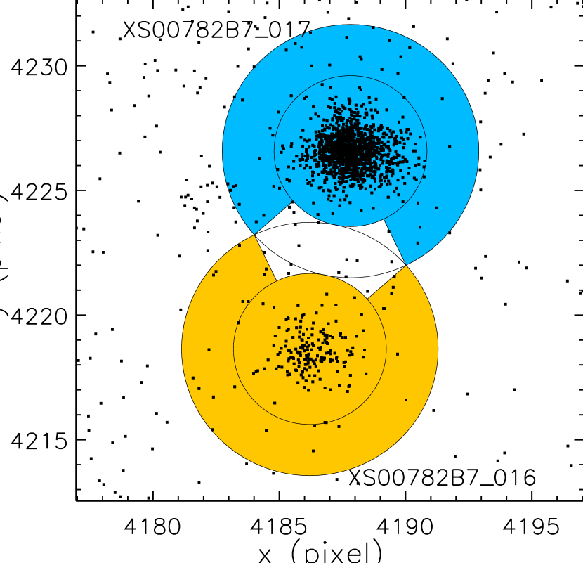
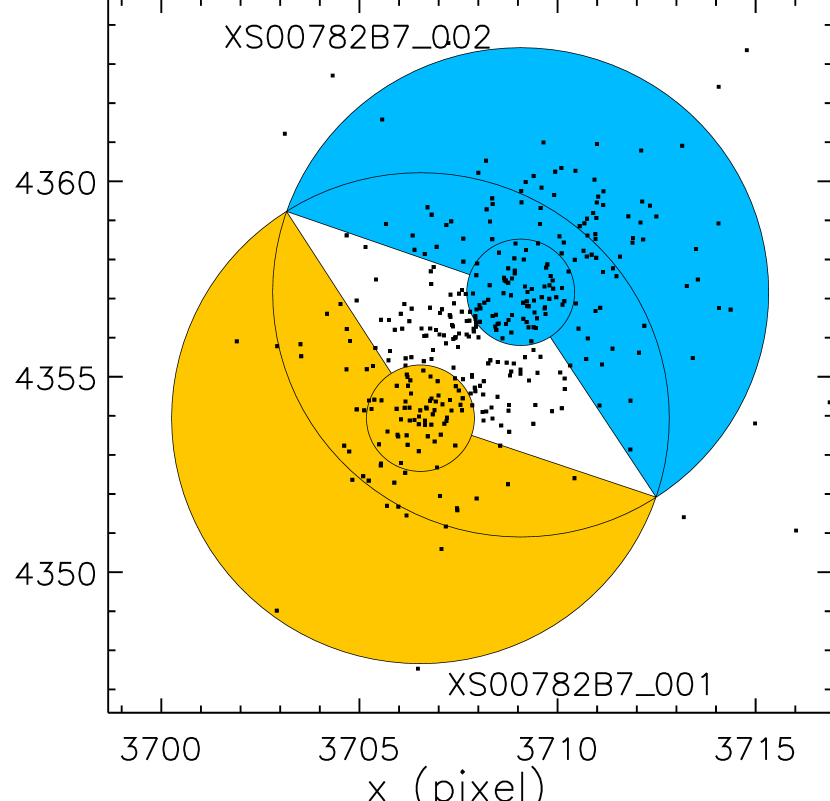
Figure 1.— Examples of overlapping source regions; relatively small overlap (left) and large overlap (right). The refined source region (yellow shade for one and blue for the other source) consists of a core and the uncommon pie sector. In the case of XS00782B7_001 and XS00782B_002 (right panel), this refinement in aperture photometry reveals these two sources have significantly different spectral types, which are otherwise indistinguishable (see §2.2.3). See the electronic ApJ for the color version of the figure

Source regions that overlap are handled in the following manner. We divide the source region into a core (circle) and a shell (annulus). We refine the source region to be the sum of the core and a pie sector of the shell that excludes the common sector with the neighbor’s source region. The core size is determined empirically to include as many source photons as possible, while minimizing contamination from neighbors. If the source region overlaps with multiple neighbors, the core radius is determined by the nearest neighbor, and the pie sector excludes all the common sectors with the neighbors’ source regions.

Fig. 1 shows examples of overlapping source regions. The shaded region indicates the refined source region: the core and the uncommon pie sector (yellow shade for one and blue shade for the other source). In the left panel of Fig. 1 where the overlap is relatively small, the core region does not overlap with the neighbor’s source region. In the right panel, the core radius is set to be one-third of the distance between two sources due to relatively large overlap. Simple aperture photometry using the source region with $r\leq\mbox{$r_{95\%}$}$ produces almost identical spectral properties for the two sources in the right panel; XS00782B7_001 and XS00782B7_002. Aperture photometry employing the refined source region reveals a significant difference in the spectral types of these two sources (§2.2.3 and Fig. 4).

Note that the above correction for overlapping source region is modified from the original correction implemented in XPIPE (K04; Kim 2005) in order to allow relatively high source counts and easy quantile analysis (§2.2.3).

XPIPE sets various flags on each source detected by wavdetect depending on source properties such as proximity to a chip boundary. These flags allow us to determine the validity of each source. A subset of the flags are set manually by the V&V step (K04) in order to remove residual artificial sources such as those stemming from frame transfer streaks during read-outs. PXP inherits the XPIPE V&V-based source flag information and sets additional flags relevant to the aperture photometry routine in PXP.

Table 5 lists the flags and their definitions. For example, when the source region overlaps with neighbors’ source regions, we flag the source (141). If the core for the refined source region is very small ($r_{c}<\mbox{$r_{39\%}$}$) and the area of the uncommon pie sector is less than 30% of the shell area, we return to the simple aperture photometry because the refined aperture photometry is also subject to a large uncertainty and we set another flag (142) on the source for further analysis.

For the initial analysis, we extract three groups of source properties from the aperture photometry: source count and rates, flux, and quantiles.

Table 5Source Flags used in ChaMPlane Analysis

Type	Flag	Definition
False sources by V&Va	111	False source by hot pixels or by bad bias values
	112	False source by bad columns
	113	False source due to readout streaks by a very strong source
	114	False source by the FEP 0/3 problemb
	115	Double source detected by the PSF effectc
	121	Other spurious sources
Valid sources but source properties may be subject to a large uncertaintyd	141	Source region overlaps with neighbors’ source regions
	142	No refinement on source region due to severe source region overlap
	143	Background region overlaps with neighbors’ source regions
	146e	Source at the chip boundary
	147	Pile-up candidate ($\geq$ 100 cts/ksec)
	148	Uncertain source position by flag = 115c
Other cases	151	Source is extended
	153	Target of the observation
	154	Sources in the target region (e.g. point sources in a target cluster)
	157f	The same source is found in other observations
	158f	The same source is found in the stacked image

Notes. — XPIPE assigns a very similar set of flags (see Table 3 in K04), but we redefine a full set of flags for PXP because many flags depend on the details of the aperture photometry. To avoid confusion with the XPIPE flags, the PXP flag IDs $\geq 100$ and the XPIPE flag IDs $<100$.
^aProvided by the XPIPE Validate and Verify (V&V) record.
^bhttp://cxc.harvard.edu/ciao/caveats.
^cSee Fig. 7 in K04.
^dThese flags are set automatically. The 95% PSF size for source region is based on psfsize_20010416.fits (§2.2).
^eWhen the source region contains any pixel that has 10% or less of the maximum exposure value of the CCD.
^fThese flags are set automatically, based on Eq. (6).

2.2.1 Net counts and net count rate

For a given band, the number of net counts ($N\mbox{$\rm{}_{net}$}$) of a source without source region overlap is derived from the number of counts ($N\mbox{$\rm{}_{src}$}$) in the source region (with area $A_{S}=\pi\mbox{$r^{2}_{95\%}$}$), the number of counts ($N\mbox{$\rm{}_{bkg}$}$) in the background region (with area $A_{B}$), and the relative ratio ($R$) of the two areas scaled by the exposure map ($e_{p}$) values of the regions.

$$N\mbox{$\rm{}_{net}$}=N\mbox{$\rm{}_{src}$}-R\ N\mbox{$\rm{}_{bkg}$},\ \mbox{\ and\ \ }R=\frac{A_{S}\ \overline{e_{p}}|_{p\in A_{S}}}{\sum_{p\in A_{B}}e_{p}},$$ (1)

where $\overline{e_{p}}|_{p\in A}$ is the mean value of $e_{p}$ in $A$. Note that ideally $A\ \overline{e_{p}}|_{p\in A}=\sum_{p\in A}e_{p}$, but when $A$ is small (often true for source regions), the former produces more reliable estimates of the exposure sum because exposure maps are usually pixellated.

In the case of source region overlap, we assume azimuthal symmetry of the PSF and we derive $N\mbox{$\rm{}_{src}$}$ from the number of counts ($N\mbox{$\rm{}_{core}$}$) in the core and the number of counts ($N\mbox{$\rm{}_{pie}$}$) in the uncommon pie sector (with area $A_{P}$),

$$N\mbox{$\rm{}_{src}$}=N\mbox{$\rm{}_{core}$}+R^{\prime}\ N\mbox{$\rm{}_{pie}$},\ \mbox{\ and\ \ }R^{\prime}=\frac{A^{\prime}_{P}+A_{P}}{A_{P}},$$ (2)

where $A^{\prime}_{P}$ is the area of the common pie sector and we use Eq. (1) for $N\mbox{$\rm{}_{net}$}$.

The net count rate ($r\mbox{$\rm{}_{net}$}$) is defined by the ratio of the number of net counts to the exposure time ($T$) and it is scaled by the ratio of the mean value of exposure map within the source region to the value at the reference point, $\mbox{max}(e_{p})$,

$$r\mbox{$\rm{}_{net}$}=\frac{N\mbox{$\rm{}_{net}$}}{T}\frac{\mbox{max}(e_{p})}{\overline{e_{p}}|_{p\in A_{S}}}.$$ (3)

The max($e_{p}$) is the maximum of the exposure map value of the chip. This exposure map scaling is implemented for easy conversion from count rate to flux regardless of source position on the chip.

PXP calculates the number of net counts, the net count rate and their errors for each source in the $S_{C}$, $H_{C}$, $B_{C}$, and $B_{X}$ bands (Table 2).

2.2.2 Flux

To estimate the X-ray flux from a source, PXP uses sherpa to calculate the count rate to flux conversion factor. To do so, we need an accurate detector response function, a column density ($N_{\mbox{\scriptsize H}}$) to the source, and a reliable spectral model for X-ray emission.

The detector response function varies with source position on the chip. However, we simply use the redistribution matrix file (RMF) and the auxiliary response file (ARF) calculated at the reference point (exposure maximum) for each CCD because spatial variation of RMFs and ARFs is relatively small (usually $<5\%$). Note that the ARFs generated by mkarf account for the known temporal degradation of the low energy efficiency of ACIS detectors. For stacked data, we simply use the RMFs and ARFs of the base observation for the initial estimation.

For the spectral model or column density, as we do not have an a priori prescription or estimate for most detected sources, we use several simple models to estimate the source flux, viz. power-law models with $\mbox{$\Gamma$\mbox{$\rm{}_{ph}$}}=$1.7, 1.4 and 1.2 likely to be appropriate for accretion powered sources such as background AGN and X-ray binaries. We also use Raymond-Smith, MeKaL, thermal Bremsstrahlung, and Black Body – all with $kT=1.0$ keV – for thermal sources (e.g., coronal sources).

For the column density $N_{\mbox{\scriptsize H}}$, we employ two models; Schlegel et al. (1998) and Drimmel et al. (2003). In general, Schlegel et al. (1998) provide realistic estimates of total Galactic extinction, but their estimation near the Galactic Plane ($|b|<5\mbox{${}^{\circ}$}$) is not as reliable as in high-latitude fields. The model may overestimate the extinction due to incomplete correction for point source contributions in the Plane. Drimmel et al. (2003) provide a 3-D model of extinction in the Galaxy, which is useful for Galactic sources with known distances. However, their model may underestimate the total column density since it does not include contributions from all known molecular clouds.

As shown in Table 1, the $N_{\mbox{\scriptsize H}}$ estimates by Schlegel et al. (1998) for the selected anti-GC fields are indeed larger (by $\sim 10-200\%$ depending on the fields) than the estimates by Drimmel et al. (2003). According to Drimmel et al. (2003), their model is normalized so that the two models agree well for high latitude fields, but as indicated by large disagreements, both models suffer relatively large uncertainties at low latitude fields.

In addition to intrinsic uncertainties in the models, we do not know the distance of most of ChaMPlane sources. Therefore, PXP calculates the $N_{\mbox{\scriptsize H}}$ value at each source position for both models, assuming the total column density along the line of the sight. The angular resolutions of the models are $\sim 6^{\prime}$ for Schlegel et al. (1998) and $\sim 20^{\prime}$ for Drimmel et al. (2003), and $N_{\mbox{\scriptsize H}}$ is then interpolated on this grid to the source position. We use $\mbox{$N_{\mbox{\scriptsize H}}$}/E(B-V)=5.8\times 10^{21}$ cm^-2/mag (Bohlin et al., 1978) to convert Schlegel et al. (1998) values of E(B-V) and $\mbox{$N_{\mbox{\scriptsize H}}$}/A(V)=1.79\times 10^{21}$ cm^-2/mag (Predehl & Schmitt, 1995) with the “rescaled” option to account for the small angular scale dust structure in using the Drimmel et al. (2003) maps.

For each source, by default, PXP estimates the X-ray flux in the $S_{C}$, $H_{C}$, $B_{C}$ and $B_{X}$ band using all seven spectral models and two extinction models. PXP is designed to allow easy addition of new spectral or extinction models and it can also assign a separate spectral and extinction model unique to each source. In future, for sources with information on spectral type, distance or column density, the X-ray flux will be revised accordingly. For example, one can estimate the column density to a source from the quantile analysis of the X-ray spectrum if one can assign a reliable spectral model to the source (see §3.3).

2.2.3 Quantiles

The survey strategy ultimately relies on the optical or IR spectroscopy to identify the nature of low luminosity X-ray sources discovered from the Chandra archival data (Grindlay et al., 2005). However, even at the R $\sim$ 24.5 optical ChaMPlane limits (Zhao et al 2005), we do not find counterparts for about half the ChaMPlane X-ray sources (e.g. Table 7). In these cases, we rely on the X-ray data for a clue to the source nature. Since the majority of the sources possess only $\sim$10–20 counts it is important to use a technique that is sensitive to low-count statistics and with minimum count-dependent bias.

In the ChaMP project, source classification by the X-ray data relies on the X-ray hardness ratio and X-ray colors (K04). These quantities are based on a particular choice of three sub-energy bands (0.3–0.9, 0.9–2.5, and 2.5–8.0 keV). In ChaMPlane, it became quickly clear that this band choice is not optimal for many highly-absorbed Galactic sources or very soft coronal sources due to count-dependent selection effects intrinsic to this particular choice of bands (Hong et al., 2004). In fact, for X-ray hardness ratio or colors, there is no single set of energy bands that can effectively describe the diverse classes of X-ray sources found in Galactic Plane fields.

Therefore, for ChaMPlane, we employ a new spectral classification technique, quantile analysis, to acquire more versatile measures of X-ray characteristics of sources. First introduced by Hong et al. (2004), the quantile analysis employs various quantiles (median, terciles, quartiles, etc) of spectral distributions to reveal and classify various spectral features and shapes. Hong et al. (2004) illustrate the technique using a quantile-based color-color diagram (QCCD), where the median of the distribution is used to indicate the overall hardness and the quartile ratio is used to classify the general shape (concave-up and -down) of the spectrum.

The quantile analysis does not require sub-division (binning) of the energy range, and it takes full advantage of energy resolution of the instruments. Therefore, quantile analysis is free of any selection effects inherent in the conventional approaches, and source classification by QCCDs is uniformly more sensitive than that by conventional X-ray color-color diagrams (Hong et al., 2004).

For a given source, PXP feeds the lists of photon energies in the source and background regions together with the weighted ratio of the two regions ($R$) into the routine quantile.pl (Hong et al., 2004). In the case of source region overlap, we use events in the refined source region (the core plus the uncommon pie sector) and the area ratio $R$ is given by

$$R=\frac{(A_{C}+A_{P})\ \overline{e_{p}}|_{p\in A_{S}}}{\sum_{p\in A_{B}}e_{p}},$$ (4)

where $A_{C}$ is the area of the core and $A_{P}$ the area of the uncommon pie sector. For example, without refining the source region, the two sources in the right panel of Fig. 1 show almost identical spectral properties due to source photon mixing; the median energy $E_{50\%}$ = 3.96(11) keV for XS00782B7_001 and $E_{50\%}$ = 3.96(09) keV for XS00782B7_002. However, the above-refined aperture photometry reveals their spectral type is indeed quite different; $E_{50\%}$ = 4.29(15) keV for XS00782B7_001 and $E_{50\%}$ = 3.73(12) keV for XS00782B7_002 [diamonds in Fig. 4 (c)]

For each source, PXP generates five quantiles, median ($m=\mbox{$Q_{50}$}$), terciles ($Q_{33}$ and $Q_{67}$), quartiles ($Q_{25}$ and $Q_{75}$), and their errors in two broad energy bands, $B_{X}$ and $B_{C}$. Examples of quantile analysis on the anti-GC fields are provided in section 3.3.

2.3. Positional uncertainty and cross-correlating X-ray sources

The wavdetect routine provides the sky position and positional errors of each source, but wavdetect underestimates the positional errors because the inputs to wavdetect are not ideal. For example, we use symmetric PSFs for wavdetect but the PSFs become asymmetric at large off-axis angles. In addition, the exposure map is calculated at 1.5 keV for practical purposes (no information about the source spectrum is available in advance; the effective area as a function of energy peaks at 1.5 keV) but no ChaMPlane source is expected to exhibit purely 1.5 keV emission. For optical or IR identification of X-ray sources, we need a more reliable estimate for the uncertainty of wavdetected source positions. To do so, we have performed SAOSAC & MARX simulations.

We generate a series of simulated sources evenly spaced in radial ($1^{\prime}$ spacing out to $\sim 10^{\prime}$) and azimuthal directions (15^∘) from the aim point. We simulate the Chandra High Resolution Mirror Assembly (HRMA) PSF using SAOSAC and simulate ACIS-I detection using MARX. The source photons are sampled from a power law model with $\mbox{$\Gamma$\mbox{$\rm{}_{ph}$}}=1.5$ and $\mbox{$N_{\mbox{\scriptsize H}}$}=3\times 10^{20}$ cm^-2 and the background photons from the Markevitch ‘period B’ ACIS-I background dataset (acisi_B_i0123_bg_evt_230301.fits). The total source photons for a given source ranges from 5 to 1000 counts, and the background is integrated over 10 ksec (for $<15$ count sources) or 20 ksec (for $\geq 15$ count sources).

We apply wavdetect to the simulated data, using a simplified version of XPIPE, and compare the wavdetected source positions with the true positions. Fig. 2 shows the size of such calculated 95% error circles (95% of the true source positions lie within the circle) as a function of the offset from the aimpoint ($D\mbox{$\rm{}_{offset}$}$ in arcmin) and the number of net counts ($c\mbox{$\rm{}_{n}$}$). Based on this result, we generate the empirical formula for 95% error circle $P\mbox{$\rm{}_{err}$}$ of the wavdetected source position.

$$P\mbox{$\rm{}_{err}$} =0.25^{\prime\prime}+\frac{0.1^{\prime\prime}}{\log_{10}(c\mbox{$\rm{}_{n}$}+1)}\left[1+\frac{1}{\log_{10}(c\mbox{$\rm{}_{n}$}+1)}\right]$$

$$+ 0.03^{\prime\prime}\left[\frac{D\mbox{$\rm{}_{offset}$}}{\log_{10}(c\mbox{$\rm{}_{n}$}+2)}\right]^{2}+0.0006^{\prime\prime}\left[\frac{D\mbox{$\rm{}_{offset}$}}{\log_{10}(c\mbox{$\rm{}_{n}$}+3)}\right]^{4}.$$ (5)

The simulations are performed for ACIS-I detectors only and we employ the formula for both ACIS-I and ACIS-S observations. For very small count sources ($c\mbox{$\rm{}_{n}$}\ll 5$), the error estimate made by the above formula can be unreasonably large, so we limit the positional error as $P\mbox{$\rm{}_{err}$}\leq r\mbox{$\rm{}_{95\%}$}$ because $P\mbox{$\rm{}_{err}$}\approx r\mbox{$\rm{}_{95\%}$}$ for a one count source with no background.

For matching with optical or IR sources, we use the $P\mbox{$\rm{}_{err}$}$ along with other relevant information such as boresight offset, optical error circle, etc (Laycock et al., 2005; Zhao et al., 2005). For the X-ray data base, PXP generates an index table that cross-correlates potentially identical sources that appear in multiple observations of the same region. First, we correct the X-ray source positions using the known aspect offset for each observation.⁴ Next, we consider two sources to be potentially identical (and also set flag=157), when the distance ($\Delta\mbox{$\rm{}_{12}$}$) between the sources is less than the quadratic sum of the error radius of both sources, i.e.

$$\Delta\mbox{$\rm{}_{12}$}\leq(P^{2}_{\mbox{\scriptsize err1}}+P^{2}_{\mbox{\scriptsize err2}}+0.7^{2}\mbox{$\times$}2)^{0.5},$$ (6)

where the constant term is added to account for the accuracy of the absolute astrometry (0.7^′′ for 95% error for each observation) after the aspect offset correction. Note Eq. (6) is used only for cross-correlating (or boresighting) X-ray to X-ray observations; for matching with optical or IR sources, see (Laycock et al., 2005; Zhao et al., 2005).

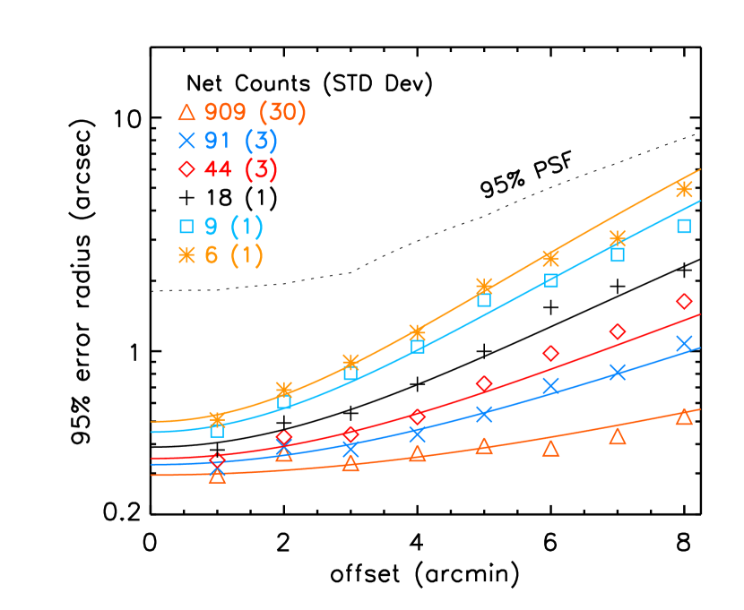
Figure 2.— 95% inclusion radius ($P\mbox{$\rm{}_{err}$}$) for uncertainties of wavdetected source positions by SAOSAC & MARX simulations; the data points are simulated results for a given number of detected net counts reported by wavdetect, and the solid lines are the visually chosen empirical formula, Eq. (5). The dotted line represents 95% PSF radius ($r\mbox{$\rm{}_{95\%}$}$, §2.3), used for the upper limit of $P\mbox{$\rm{}_{err}$}$.

3. Initial results for the anti-GC fields

In the following, we consider the results from the unstacked data.

3.1. Source statistics

Table 6 summarizes the initial X-ray results of the ChaMPlane survey on the 15 selected (see Table 1) anti-GC observations. The table shows the summary of source counts at each level of the analysis. The levels are devised to select valid sources and to increasingly (with level) restrict systematic errors.

The wavdetect routine detected 1028 sources in the 15 selected anti-GC observations (level 0). After careful selection of sources by the flag information and V&V, we found 921 reliable sources (level 1) in these regions. To interpret the results without concern for anomalies arising far from the aim point, we further limit the source list. In level 2, we use only data from CCDs 0, 1, 2, and 3 for ACIS-I observations, and CCD 2, 3, 6, and 7 for ACIS-S observations. In level 3, we select sources within 400^′′ of the aim point for ACIS-I observations, and all of CCD 7 for ACIS-S observations. Note that level 3 uses only front-illuminated (FI) CCDs for ACIS-I and only one back-illuminated (BI) CCD for ACIS-S observations.

The last three columns in Table 6 list the number of sources that need special attention for further analysis: the same sources found in multiple observations of the same field (flag=157; i.e., the first 2 observations listed in Table 1), sources that may be piled-up (flag=147), and sources with their source region overlapping with neighbors’ source region (flag=141).

Table 6Summary of Source Numbers for 15 selected anti-GC observations (7 ACIS-I, 8 ACIS-S Observations.)

			Number of Sources				Speciala
	Stage	Selection Rules	ACIS-I	ACIS-S	Total		multiple	pile-up	overlap
level 0	wavdetect	Everything	448	580	1028		18$\times$2	3	28
level 1	Select valid sourcesb	Flag $\neq$ 11x, 12x, nor 146	431	490	921		18$\times$2	3	20
		CCD 0, 1, 2, 3 for ACIS-I Obs.,
level 2	CCD selection	CCD 2, 3, 6, 7 for ACIS-S Obs.	409	445	854		18$\times$2	2	16
		in $B_{C}$	330	396
	SNR $\geq 3$	in $S_{C}$	214	316
		in $H_{C}$	189	213
		$<$400′′ for ACIS-I Obs.,
level 3	Off-axis limit	CCD 7 for ACIS-S Obs.	276	242	518		16$\times$2	2	12
		in $B_{C}$	214	210
	SNR $\geq 3$	in $S_{C}$	131	169
		in $H_{C}$	123	110

Notes. — See Table 5 for flag definitions.
^aSpecial attention required: sources found in multiple observations of the same field (flag=157), potential pile-ups (flag=147), and source region overlap (flag=141). No source with flag=142 (severe source region overlap) is found in these fields
^bRemoves extended sources and other apparently false sources. For the case of sources near a chip boundary (flag=146), they may be valid sources, but we do not include them for level $\geq$ 1 analysis because their position and source properties are subject to large uncertainties.

In the following, we go over the basic X-ray properties of the above sources. The complete source catalog as well as access to the X-ray and optical images and optical photometry data for probable IDs (see Grindlay et al 2005 for examples) is available on-line.

3.2. Source distribution

We derive the log$N$-log$S$ distribution to review the analysis procedure and for an initial analysis of the nature of the source population. In general, making an estimate of the unabsorbed flux for sources in the Galactic Plane fields is more difficult than for high-latitude sources because of the diverse and unknown spectral types, the higher column density and its strong dependence on the usually unknown distances to the Galactic sources. Therefore, the derivation and interpretation of the log$N$-log$S$ distributions for ChaMPlane sources are not trivial. For the initial analysis, we follow a practice similar to the one done for ChaMP (K04), which allows us to verify the consistency of the analysis and to compare the results directly with the high-latitude ChaMP results. We generate the sky coverage and the log$N$-log$S$ distribution in the $S_{C}$ and $H_{C}$ band. To simplify the analysis, we use only the level 3 data set. We also exclude the original target (and point sources in the target region if the intended target contains diffuse emission or a cluster of X-ray sources; flag=154) of each observation to maintain the serendipitous nature of the survey. For example, in the NGC 1569 field (a galaxy, Obs. ID 782), we consider the point sources within the 3.6^′ diameter circle from the galaxy center as a part of target, and in the 3C 123 field (a quasar, Obs. ID 829), two sources nearby 3C 123 are also considered so.

3.2.1 Sky Coverage

To calculate the amount of sky covered, we adopt a relatively simple but accurate procedure (Cappelluti et al., 2005). First, we generate a background-only image from event files for a given band. Using the valid source list (level 1), we remove the photons in the source regions and fill the regions with counts consistent with the neighboring background using dmfilth. Note we keep the photons in the source region of the target (and sources in the target region if the target is extended) in the background-only image because we exclude these sources in counting the number of sources for log$N$-log$S$. Second, for a given position in a CCD, using the exposure map and the background image, we estimate the count rate limit ($r_{l}$) for detection at a given signal-to-noise ratio (SNR$=\sigma$) by

$$r_{l}=\sigma\frac{1+(0.75+N_{B})^{1/2}}{T}\frac{\mbox{max}(e_{p})}{\overline{e_{p}}|_{p\in A_{B}}},$$ (7)

where $N_{B}$ is the background count in the source region, $T$ the exposure time, $\sigma$ = 3 and we use Gehrels’ approximation for the errors (Gehrels et al., 1986).

We need to convert $r_{l}$ to the equivalent flux in order to calculate the sky coverage as a function of flux. Note that $r_{l}$ is scaled by the exposure map in the same way as $r\mbox{$\rm{}_{net}$}$ in Eq. (3). Therefore, one can use the same rate-to-flux conversion factor in the previous section (§2.2.2) to convert $r_{l}$ to the equivalent flux. However, there is no unique conversion from the count rate to un-absorbed flux because sources in the Galaxy can be at any distance from the Earth and the column density changes with the distance. As for direct comparison with the ChaMP results, we again assume the full column density along the line of the sight provided by the extinction models. Since Schlegel et al. (1998) may overestimate and Drimmel et al. (2003) may underestimate the total extinction along the line of the sight, we use both models (insets in Fig. 3).

As for spectral models, we employ a power-law emission model with $\mbox{$\Gamma$\mbox{$\rm{}_{ph}$}}=1.7$ for the $S_{C}$ band and $\mbox{$\Gamma$\mbox{$\rm{}_{ph}$}}=1.4$ for the $H_{C}$ band sources as in ChaMP (K04). These assumptions for spectral and column density models are more relevant for background AGN sources than for Galactic sources.

Using the rate-to-flux conversion factor and Eq. (7), one can assign the flux limit for $\sigma=3$ at any position in the detector. For a given flux, the sky coverage is derived by summing up the detector area where the calculated flux limit is less than the given flux. In summation, we only include the level 3 region where exposure map is greater than 10% of the maximum of the CCD to meet the source selection criterion (flag $\neq$ 146).

3.2.2 log$N$-log$S$

To be consistent with the sky coverage calculation ($\sigma\geq 3$), for a given band, we count the number of sources with SNR$\geq 3$ for the log$N$-log$S$ distribution except for the target and sources in the target region, where

$$\mbox{SNR}=\frac{N\mbox{$\rm{}_{net}$}}{1+(0.75+N\mbox{$\rm{}_{src}$}-N\mbox{$\rm{}_{net}$})^{1/2}}.$$ (8)

Fig. 3 shows the log$N$-log$S$ distribution of the sources in the anti-GC fields. The solid line with the (yellow) shade is for the extinction model by Schlegel et al. (1998), and the dotted line with the (red) shade is for the model by Drimmel et al. (2003). The shading represents the statistical uncertainties ($\pm 1\sigma$) of the distribution. The ChaMP results are shown as a thin (blue) solid line without any shade in the plots. Table 7 summarizes the current status of source classification (only $\sim$ 6 – 17%) by optical imaging and spectrocopy for the sources in Fig. 3.

In Fig. 3, for a given spectral and extinction model, the results for the ACIS-I and ACIS-S observations agree within $\leq 2\sigma$ overall, and they exhibit better agreement ($\leq 1\sigma$) where the number of sources is sufficient so that the statistical fluctuations are not too overwhelming ($S_{0}<1\times 10^{-14}$ erg/sec/cm² in the $S_{C}$ band and $S_{0}<3\times 10^{-14}$ erg/sec/cm² in the $H_{C}$ band).

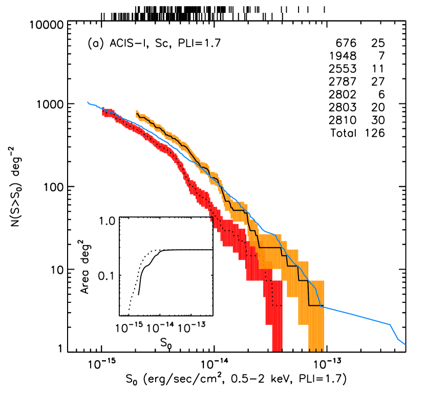
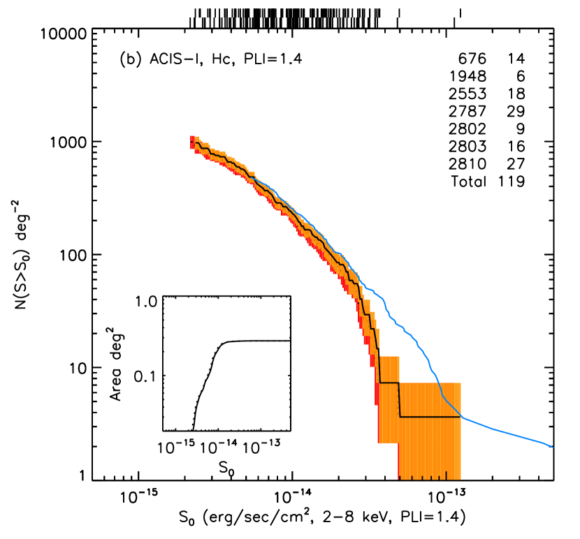
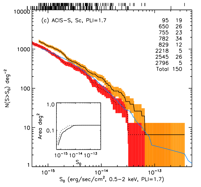
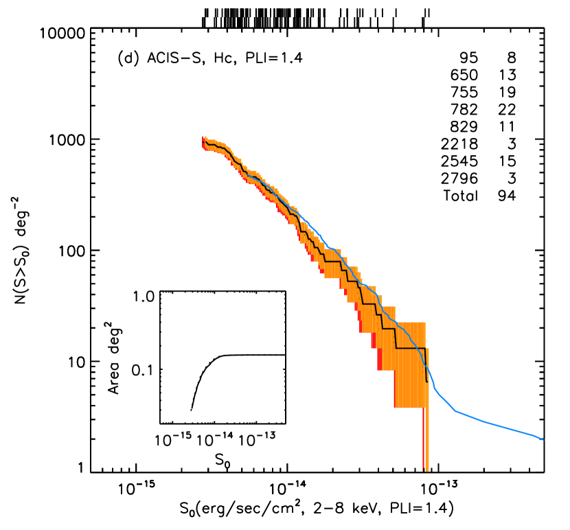
Figure 3.— The log$N$-log$S$ distributions of the X-ray sources in the 15 anti-GC observations ($90\mbox{${}^{\circ}$}<l<270\mbox{${}^{\circ}$}$): (a) ACIS-I observations in the $S_{C}$ band, (b) ACIS-I in $H_{C}$, (c) ACIS-S in $S_{C}$, and (d) ACIS-S in $H_{C}$. The solid line with the (yellow) shade is for the extinction model by Schlegel et al. (1998), and the dotted line with the (red) shade is for the model by Drimmel et al. (2003). The shading represents the statistical uncertainties ($1\sigma$) of the distribution. The thin (blue) solid line is the extra-Galactic result from ChaMP (K04). The inset shows the sky coverage: the solid line from the model by Schlegel et al. (1998), and the dotted line from Drimmel et al. (2003). The top right list in each plot indicates the Obs. IDs and the number of sources with SNR $\geq 3$. The targets of each observation are excluded. The vertical black bars above each plot show the actual source distribution by flux assuming the model by Schlegel et al. (1998) (top row) and the flux distribution assuming the model by Drimmel et al. (2003) (bottom rows). See the electronic ApJ for color version of the plots.

Because of the relatively poor statistics, it is premature to attribute differences between the ACIS-I and ACIS-S observations to any systematic bias in the analysis. For example, in the case of the $S_{C}$ band [Fig. 3 (a) & (c)], the log$N$-log$S$ distributions expectedly show a strong dependence on the extinction models, which differ by as much as a factor of 3 (Table 1). For Galactic populations, the extinction depends strongly on the distance to the sources. In addition, the assumed power law emission model ($\Gamma$_ph =1.7) may not properly describe the X-ray emission from these sources (§3.3). For soft coronal sources (§3.3), the assumed power law emission model likely underestimates the source flux and thus their contribution to the log$N$-log$S$ distribution, particularly in the soft band (shifting the log$N$-log$S$ distribution to the left in the plot).

The unknown spectral model and the inaccurate extinction estimate dominate the uncertainty of the log$N$-log$S$ distributions in the $S_{C}$ band. Nonetheless, we expect our anti-GC results to exhibit an excess relative to the ChaMP log$N$-log$S$ distribution. We suspect the extinction model of Drimmel et al. (2003) underestimates the total Galactic $N_{\mbox{\scriptsize H}}$ values for at least a subset of the fields.

In the case of the $H_{C}$ band [Fig. 3 (b) & (d)], the log$N$-log$S$ distributions for the anti-GC fields are not sensitive to the extinction models, and the results are consistent with the ChaMP log$N$-log$S$ distribution within the statistical limit. This indicates that most of the strong hard sources are background AGNs. For example, judging from the statistical uncertainty of the log$N$-log$S$ distributions, we estimate that for $S>S_{0}=2\mbox{$\times$}10^{-14}$ erg/sec/cm², only less than $\sim$ 20% of the sources are Galactic in Fig. 3 (b) & (d).

It is premature to draw any conclusion from source classification (Table 7 or Table 8) because only $\sim 10$% of the sources in Fig. 3 (b) & (d) are identified as of this writing. However, the above log$N$-log$S$ results are consistent with source classification in Table 7 because, among 8 sources (out of 15 classified sources in the $H_{C}$ band) that have $S>2\mbox{$\times$}10^{-14}$ erg/sec/cm² and SNR $\geq 3$ in the $H_{C}$ band, 7 sources are quasars and only one is Galactic. Note that in the above comparison, we need a limit on $S$ to alleviate the selection effects arising from spectral difference between stars and quasars in Table 7.

Assuming the extinction model by Schlegel et al. (1998) is correct or at least does not underestimate the total Galactic $N_{\mbox{\scriptsize H}}$ value, let us compare the results using Schlegel et al. (1998) in Fig. 3. The log$N$-log$S$ distributions in the $S_{C}$ band shows a larger excess compared to the ChaMP result than the distributions in the $H_{C}$ band. Several reasons may explain these differences. First, the X-ray emission of many Galactic sources, e.g. coronally active stars – that are detected in ChaMPlane but not in ChaMP– is relatively stronger in the soft band. Although only $\lesssim$ 15% of the X-ray sources are classified (Table 7), the results suggest that, as expected, the star to quasar ratio in the log$N$-log$S$ distribution of the soft band is higher than the same for the hard band. Second, for Galactic sources, the extinction and hence the unabsorbed flux is likely overestimated by the model of Schlegel et al. (1998) which can systematically shift the entire curve in Fig. 3 to the right. The effects of extinction are relatively larger in the soft than in the hard band.

Table 7Classification of Sources in Fig. 3 by Optical Imaging and Spectroscopy

	ACIS-I					ACIS-S
	(a) $S_{C}$		(b) $H_{C}$			(c) $S_{C}$		(d) $H_{C}$
Total	126		119			150		94
aMatching performed	89		76			124		79
bOptical Matches	65	(6)	38	(5)		71	(3)	33	(0)
cSpectrum Observed	35		23			41		19
Identified as Stars	15		5			24		3
Quasars	8		4			3		3
Galaxy	1		0			0		0
Unclear	11		14			14		13

Notes. — The log$N$-log$S$ distributions in Fig. 3 exclude targets of each observation.
^aAs of this writing, source classification with optical spectroscopies is performed for 4 ACIS-I Obs. and 6 ACIS-S Obs. among total 15 Obs. See also Zhao et al. (2005).
^b() for the number of sources with multiple matching candidates.
^cSee Rogel et al. (2005).

To derive the true Galactic log$N$-log$S$ distribution, we need to allow for the differing source spectra and distances (and thus $N_{\mbox{\scriptsize H}}$), and then re-derive the flux estimate of each source separately. In future papers, we shall incorporate additional information (e.g. from optical spectra and thus reddening) for sources whenever available for more complete log$N$-log$S$ distributions.

3.3. Source Properties by QCCD

Fig. 4 shows the QCCDs of the anti-GC field sources with $N\mbox{$\rm{}_{net}$}>40$ in $B_{X}$. The detailed description of the QCCD is found in Hong et al. (2004). In summary, the $x$-axis shows the median of the photon energy distribution ($m$) and the $y$-axis shows the ratio of two quartiles of the photon energy distribution (3 $Q_{25}$/$Q_{75}$). Note that the median $m$ is related to the median energy ($E_{50\%}$) by

$$m=\frac{E_{50\%}-E\mbox{$\rm{}_{lo}$}}{E\mbox{$\rm{}_{up}$}-E\mbox{$\rm{}_{lo}$}},$$ (9)

where $E\mbox{$\rm{}_{lo}$}$ = 0.3 and $E\mbox{$\rm{}_{up}$}$= 8.0 keV in the $B_{X}$ band (Hong et al., 2004). The top $x$-axis of the QCCD is labeled by $E_{50\%}$ and the bottom $x$-axis is the inverse hyperbolic tangent of $m$ (this allows a convenient quantity for plotting).

Fig. 4 (a) is for ACIS-I observations, overlayed with power-law model grids, and Fig. 4 (b) shows the same data with the error bars and thermal Bremsstrahlung model grids. Fig. 4 (c) and (d) are for ACIS-S observations. The figures contain sources from level 2 data for ACIS-I, and level 3 data for ACIS-S observations (see Table 6) except for two piled-up sources (PSR J0538+2817 and GK Persei). Note the difference in the grid patterns between the FI and BI CCDs, which is mainly due to relatively high detection efficiency of BI CCDs at low energies. The temporal degradation of the low energy efficiency also makes the grid patterns change (shrink). The grid patterns in Fig. 4 are averaged over the selected observations.

In Fig. 4 (a) and (c), one can roughly identify sources in a few distinct groups. In particular, the sources within the shaded (yellow) region appear to be too soft to be described by power-law models ($\mbox{$\Gamma$\mbox{$\rm{}_{ph}$}}\gtrsim 3-4$). The rest are relatively well described by power law models with conventional values for $\Gamma$_ph ($\sim$ 1 – 3) but reveal a wide range of extinctions. In Fig. 4 (b) and (d), one can see the very soft sources are better described by thermal models ($kT\lesssim 1$ keV), which indicates many of these sources are most likely to be stellar coronal emission sources (stars). The hard sources that are better described by the power law models are likely accreting X-ray sources and are predominantly background AGN but can also include accretion-powered compact binaries (e.g. cataclysmic variables; see Grindlay et al 2005).

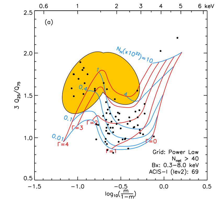
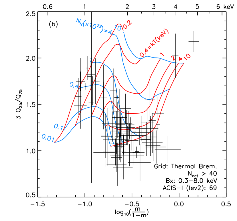
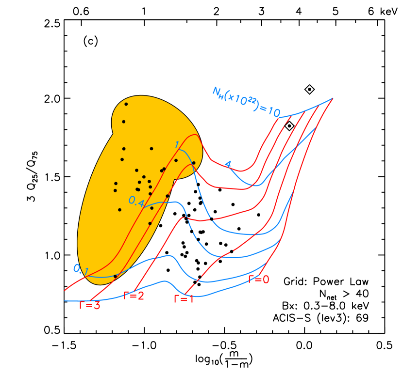
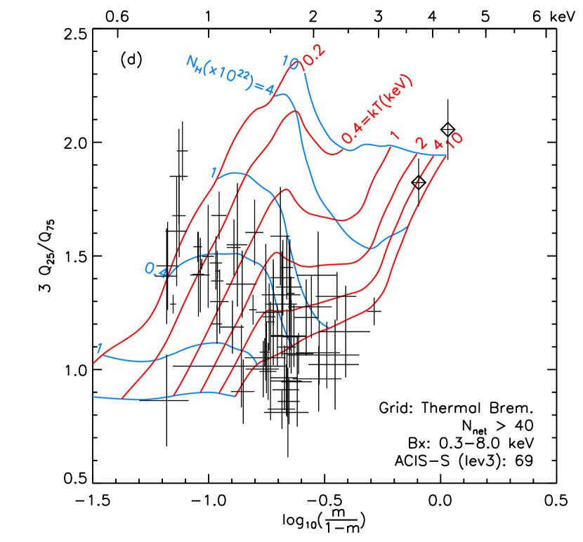
Figure 4.— QCCDs for the anti-GC sources ($N\mbox{$\rm{}_{net}$}>40$ in $B_{X}$, including targets): (a) ACIS-I observations, overlayed with power law model grids, (b) ACIS-I with error bars and thermal Brems. model grids, (c) ACIS-S, overlayed with power law model grids, and (d) ACIS-S, with error bars and thermal Brems. model grids. The power law model grids are for $\Gamma$_ph = 0, 1, 2, 3 & 4 and $N_{\mbox{\scriptsize H}}$ = $10^{20},10^{21},4\times 10^{21},10^{22},4\times 10^{22}$ & $10^{23}$ cm^-2, and the thermal Brems. model grids for $kT$ = 0.2, 0.4, 1, 2, 4 & 10 keV and the same $N_{\mbox{\scriptsize H}}$. The quantiles are calculated in the $B_{X}$ band. The ACIS-I observations contain sources from CCD 0, 1, 2, & 3 (level 2, FI), and the ACIS-S from CCD 7 (level 3, BI, see Table 6) except for the piled-up sources. In the left panels, sources in the shaded(yellow) regions are too soft to be described by power-law with physically reasonable $\Gamma$_ph and are likely dominated by stellar coronal emission sources (stars). Diamonds in (c) and (d) indicate the two example sources in the right panel of Fig. 1; XS00782B_001 and XS00782B_002. See electronic ApJ for color version of the figure.

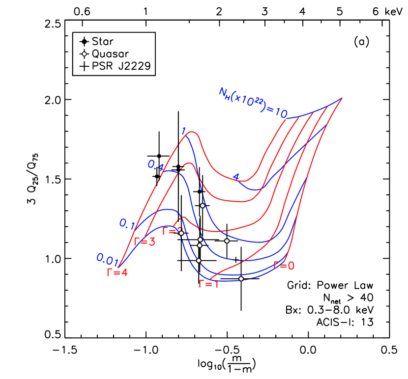
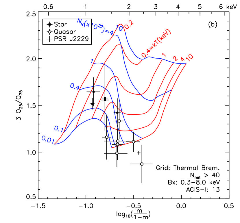
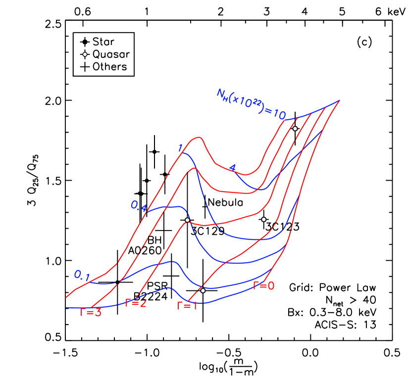
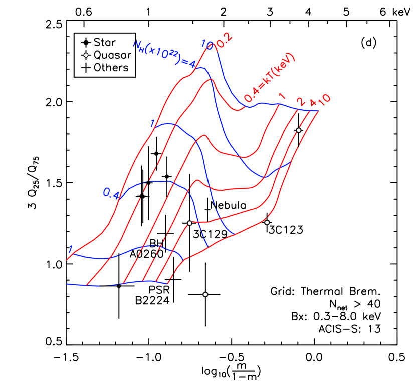
Figure 5.— The same QCCDs as in Fig. 4 but only with the optically identified sources (Rogel et al., 2005) or known sources ($N\mbox{$\rm{}_{net}$}>40$ in $B_{X}$). The solid circles are stars and the open circles are background quasars and the rest are black hole binaries, pulsars, etc. See Table 8 for the complete source list of the figure.

Table 8List of optically identified or known sources with $N\mbox{$\rm{}_{net}$}>40$ in $B_{X}$

	Source ID	Source Name	$E_{50\%}$a		$N\mbox{$\rm{}_{net}$}\$	$r\mbox{$\rm{}_{net}$}$ in $B_{X}$
	XS	CXOPS	(keV)	$3\mbox{$Q_{25}$}/\mbox{$Q_{75}$}$	in $B_{X}$	(cts/ksec)		Source Type	Known Nameb
CCD 0,1,2,3 (FI) for ACIS-I observations
	02810B2_018	J235813.4$+$622447	2.14(23)	1.11(11)	97.7	2.4	(3)	Quasar z=1.29
	00676B3_011	J042155.1$+$324724	1.71(12)	1.33(19)	64.2	3.8	(5)	Quasar z=1.845
	00676B0_001	J042201.6$+$325728	1.39(10)	1.16(24)	63.5	3.7	(5)	Quasar z=2.203
	00676B3_018	J042123.7$+$324836	1.66(14)	1.08(17)	57.0	3.6	(5)	Quasar
	00676B2_001	J042133.8$+$325556	1.64(30)	0.99(14)	48.5	2.7	(5)	Quasar z=2.055
c	02810B0_021	J235813.2$+$623343	2.44(42)	0.87(20)	42.4	1.0	(2)	Quasar z=2.04
	00676B1_006	J042211.8$+$325604	1.67(33)	1.12(15)	41.8	2.7	(5)	Quasar z=0.65
	02787B3_002	J222905.2$+$611409	2.33(06)	0.99(02)	1972.6	21.9	(5)
d	01948B3_001	J222905.2$+$611409	2.31(13)	0.98(06)	327.4	25.2	(1.5)	Pulsar	PSR J2229+6114
	02787B1_005	J222833.4$+$611105	1.10(04)	1.52(06)	237.9	2.9	(2)
	01948B1_002	J222833.3$+$611105	1.13(12)	1.64(16)	46.8	3.5	(6)	YSO K star
	02787B0_003	J223001.4$+$611059	1.35(09)	1.56(19)	87.6	1.1	(1)
e	01948B0_001	J223001.3$+$611100	1.62(34)	1.41(76)	16.8	1.3	(4)	early K star
	02787B3_007	J222847.3$+$611214	1.65(10)	1.42(15)	79.1	1.6	(2)
e	01948B1_001	J222847.3$+$611214	1.76(21)	1.45(26)	25.4	1.8	(4)	G star
	02787B3_005	J222853.1$+$611351	1.35(07)	1.58(35)	48.0	0.5	(1)
e	01948B3_004	J222853.0$+$611351	1.40(39)	1.38(37)	8.4	0.6	(3)	G/K? star
CCD 7 (BI) for ACIS-S observations
	00829B7_002	J043704.3$+$294013	2.92(12)	1.26(06)	380.7	14.1	(8)	Quasar z=0.218	3C 123
	00782B7_002	J043125.0$+$645154	3.73(12)	1.82(10)	157.8	2.7	(2)	Quasar z=0.279
	00829B7_003	J043654.8$+$294018	1.69(25)	0.81(20)	45.1	1.7	(3)	Quasar
	02218B7_004	J044909.0$+$450039	1.45(10)	1.25(30)	47.2	2.3	(4)	Quasar	3C 129
	00829B7_022	J043718.4$+$294546	1.07(05)	1.68(10)	136.2	7.4	(7)	K star
	00782B7_042	J043003.0$+$645143	1.18(05)	1.54(12)	133.6	1.7	(2)	YSO M star
	00650B7_015	J033108.2$+$435750	0.94(03)	1.42(19)	111.3	2.0	(2)	dMe star
	00755B7_005	J222545.8$+$653833	0.95(06)	1.42(16)	75.4	1.7	(2)	dMe star
	00782B7_010	J043058.3$+$644852	1.00(04)	1.50(23)	63.7	0.8	(1)	dMe star
	00782B7_018	J043039.0$+$645013	0.78(11)	0.86(20)	40.2	0.5	(1)	dMe star
	00782B7_012	J043057.4$+$645048	1.72(04)	1.34(07)	257.8	3.1	(2)	Nebula
	00095B7_004	J062244.5$-$002044	1.17(09)	1.19(12)	99.7	3.1	(4)	BH XB	A0620-00
	00755B7_004	J222552.5$+$653535	1.25(10)	0.90(14)	83.7	1.8	(2)	Pulsar	B2224+65

^a See Eq. (9). The top $x$-axis of the QCCDs is labeled by $E_{50\%}$.
^b Ones with the known name is the target of the observation.
^c Three candidates are found for the counter part. The nearest candidate is identified as a quasar and the other two are unknown type.
^d This source is not plotted in Fig. 5 for clarity.
^e Note $N\mbox{$\rm{}_{net}$}<40$ for these sources (not shown in Fig. 5), but they are listed for comparison with the same sources found in Obs. ID 2787 with $N\mbox{$\rm{}_{net}$}>40$.

Fig. 5 shows the same QCCD plots but only with the known sources or optically identified ones (Rogel et al., 2005). Table 8 contains the complete list of the sources in Fig. 5. The solid circles indicate stars and the open circles indicate background AGNs. The rest are pulsars, black hole (BH) X-ray binary (XB), etc. The QCCD separates relatively soft stars and hard quasars even with a small number of net counts ($>$ 40 counts in $B_{X}$). Five sources in Obs. ID 2787 are also found in Obs. ID 1948. Note that their quantile values (and net count rates) from two observations are consistent, even though three sources in Obs. ID 1948 have only 16.8, 25.4 and 8.4 net counts respectively (Table 8).

4. Summary

We describe the X-ray analysis procedure for X-ray processing of ChaMPlane survey archival data using custom developed analysis tools, which can be useful for other Chandra analysis projects as well. The initial X-ray results from the analysis of the 15 selected anti-GC observations reveal a few distinct classes of sources. The detailed X-ray analysis of source distributions and source classifications for all Anticenter ChaMPlane fields, followed by Galactic Bulge and GC region fields, will be presented in subsequent papers.

5. Acknowledgements

We thank Terrance Gaetz for performing the SAOSAC and MARX simulations. We also thank Dong-woo Kim, Minsun Kim and Eunhyeuk Kim for the useful discussion and suggestions, and we appreciate help from the ChaMP team for ChaMPlane data processing/analysis. This work is supported in part by NASA/Chandra grants AR1-2001X, AR2-3002A, AR3-4002A, AR4-5003A and NSF grant AST-0098683.

References

- Baganoff et al. (2003) Baganoff, F.K. et al., 2003, ApJ, 591, 891.
- Bohlin et al. (1978) Bohlin, R.C., Savage, B.D. & Drake, J.F., 1978, ApJ, 224, 132.
- Cappelluti et al. (2005) Cappelluti, N. et al., 2005, ApJ, 430, 39.
- Drimmel et al. (2003) Drimmel, R., Cabrera-Lavers, A., & Lopez-Corredoira, M., 2003, ApJ, 409, 205.
- Freeman et al. (2002) Freeman, P.E. et al., 2002, ApJS, 138, 185.
- Gehrels et al. (1986) Gehrels, N. et al., 1986, ApJ, 303, 336.
- Grindlay et al. (2003) Grindlay, J.E. et al., 2003, AN, 324, 57.
- Grindlay et al. (2005) Grindlay, J.E. et al., 2005, submitted to ApJ.
- Humphrey et al. (2003) Humphrey, P.J. et al., 2003, MNRAS, 344, 134.
- Hong et al. (2004) Hong, J, Schlegel, E.M. & Grindlay, J.E., 2004, ApJ, 614, 508.
- Kim et al. (2004a) Kim, D.-W. et al., 2004a, ApJS, 150, 19 (K04).
- (12) Kim, D.-W. et al., 2004b, ApJ, 600, 59 (K04).
- Kim et al. (2005) Kim, E., 2005, in preparation, private communication.
- Laycock et al. (2005) Laycock, S.G.T. et al., 2005, in preparation.
- Mallat, S. (1998) Mallat, S. 1998, A Wavelet Tour of Signal Processing (London: Academic Press).
- Predehl & Schmitt (1995) Predehl, P. & Schmitt, J. H. M. M., 1995, A&A, 293, 889.
- Rogel et al. (2005) Rogel, A. et al., 2005, submitted to ApJ.
- Schlegel et al. (1998) Schlegel, D., Finkbeiner, D., & Davis, M., ApJ, 1998, 500, 525.
- Zhao et al. (2003) Zhao, P. et al., 2003, AN, 324, 176.
- Zhao et al. (2005) Zhao, P. et al., 2005, submitted to ApJ.