Chandra Multiwavelength Plane (ChaMPlane) Survey: an Introduction

Abstract

We introduce the Chandra Multiwavelength Plane (ChaMPlane) Survey, designed to measure or constrain the populations of low-luminosity (L_x $\buildrel>\over{\sim}$10³¹ erg s^-1) accreting white dwarfs, neutron stars and stellar mass black holes in the Galactic Plane and Bulge. ChaMPlane incorporates two surveys, X-ray (Chandra) and optical (NOAO 4m-Mosaic imaging), and a followup spectroscopy and IR identification program. The survey has now extended through the first 6 years of Chandra data using serendipitous sources detected in 105 distinct ACIS-I and -S fields observed in 154 pointings and covered by 65 deep Mosaic images in V, R, I, and H$\alpha$. ChaMPlane incorporates fields with galactic latitude $|b|$ $\buildrel<\over{\sim}$12^∘  and selected to be devoid of bright point or diffuse sources, with exposure time $\buildrel>\over{\sim}$20ksec, and (where possible) minimum N_H. We describe the scientific goals and introduce the X-ray and optical/IR processing and databases. We derive preliminary constraints on the space density or luminosity function of cataclysmic variables from the X-ray/optical data for 14 fields in the Galactic Anticenter. The lack of ChaMPlane CVs in these Anticenter fields suggests their space density is $\sim$3$\times$  below the value (3 $\times$  10^-5 pc^-3) found for the solar neighborhood by previous X-ray surveys. Companion papers describe the X-ray and optical processing in detail, optical spectroscopy of ChaMPlane sources in selected Anticenter fields and IR imaging results for the Galactic Center field. An Appendix introduces the ChaMPlane Virtual Observatory (VO) for online access to the X-ray and optical images and source catalogs for ready display and further analysis.

1. Introduction

The Chandra Multiwavelength Plane (ChaMPlane) Survey is a comprehensive effort to analyze systematically and archive the results from deep ($\buildrel>\over{\sim}$20-100ksec) Chandra pointings near the Galactic Plane ($|b|$ $\buildrel<\over{\sim}$12^∘). The primary science goals of ChaMPlane (described below) are to measure or constrain the low-luminosity ($\buildrel<\over{\sim}$10³⁴ erg s^-1) accretion-powered X-ray sources in the Galaxy: accreting white dwarfs in cataclysmic variables (CVs), neutron stars and black holes in quiescent low mass X-ray binaries (qLMXBs) and low-luminosity high mass X-ray binaries (HMXBs), primarily Be-HMXBs. ChaMPlane is also enabling the first high-resolution search for isolated stellar mass black holes accreting from giant molecular clouds (GMCs). A key secondary goal is the study of stellar coronal emission across the H-R diagram and in a range of Galactic environments: from the Anticenter disk to the Galactic Bulge. The survey will produce the most comprehensive database of coronal X-ray sources (stars) yet achieved, ultimately expanding the ROSAT samples (e.g. Schmitt et al 2004 and references therein) by $\sim$1-2 orders of magnitude for stars in the plane and (far) beyond the solar neighborhood. While the primary goals of ChaMPlane are to survey and study point sources, the ChaMPlane X-ray and optical image archive also contain considerable rich diffuse emission which can be accessed for further study.

ChaMPlane is also a major optical imaging (V, R, I and H$\alpha$) followup survey conducted to identify optical counterparts of the X-ray survey sources. We have used the Mosaic camera on the CTIO and KPNO 4m telescopes in a 5-year Long Term Survey Program granted to ChaMPlane (in 2000) by NOAO. The images and photometry from this survey, separately processed and archived at both CfA and NOAO, constitute some of the deepest H$\alpha$  images of the Plane in the 65 Mosaic fields (36$\,{}^{\prime}$ $\times$36$\,{}^{\prime}$ ) obtained in our NOAO survey. The ChaMPlane database at CfA links the X-ray and optical images and, when complete, will produce a legacy database for the distribution and nature of faint X-ray sources in the Galactic Plane. With initial analysis on 14 Anticenter fields now nearly complete, the fraction of sources with optical counterparts is $\sim$50%.

ChaMPlane is deeper (given diffuse emission in many fields) and of course has much higher angular resolution, permitting optical/IR identifications, than the XMM Galactic Plane survey (Motch et al 2003), ROSAT all sky survey (Voges et al 1999) or the Einstein Galactic Plane Survey (Hertz and Grindlay 1984; Hertz et al 1990). Given that Chandra is the premier high-resolution X-ray imager for at least the next decade, it is important to conduct the systematic analysis of the (many) Chandra Galactic fields to create the database needed for developing a statistical understanding of the accreting binary (white dwarf, neutron star and black hole) as well as stellar coronal X-ray content of the Galaxy. An initial description of ChaMPlane and preliminary results for the derived source number vs. flux (logN-logS) distributions and source types was given for several Galactic Bulge fields by Grindlay et al (2003) along with an initial description of the optical survey (Zhao et al 2003).

The X-ray processing is described in detail in the accompanying paper by Hong et al (2005), which presents X-ray results for the initial 14 Galactic Anticenter fields (90^∘  $\buildrel<\over{\sim}$$l$ $\buildrel<\over{\sim}$270^∘). The optical survey and photometry pipeline processing for ChaMPlane is described in the accompanying paper by Zhao et al (2005). A broad overview of both the X-ray and optical survey status, as well as portals to the archived data and source catalogs, is available from the ChaMPlane website . ChaMPlane also incorporates an extensive optical spectroscopy followup program (at WIYN, MMT, CTIO and Magellan) and infrared (IR) imaging and photometry and ultimately spectroscopy. Details are given in sections 5.2 and 5.3.

The ChaMPlane X-ray and optical surveys are now building, and releasing, significant X-ray and optical database archives of processed images and derived X-ray fluxes and colors and optical photometry. The optical database also includes photometry (V,R,I and H$\alpha$) and astrometry results for the full stellar content of all Mosaic fields acquired. The images and derived catalogs are released as initial science papers are submitted. We have developed tools for easy web access to the X-ray and optical images and derived products in the database. Examples of these tools for X-ray and optical overlays are given in the Appendix.

We first summarize the key science objectives of ChaMPlane and the criteria for selection of Chandra pointings for the survey. We then describe the X-ray processing and survey coverage obtained and then the optical-IR surveys and data products. Finally, we derive initial constraints on the CV density and/or luminosity function from X-ray/optical results for the 14 fields processed for the Anticenter. In the Appendix we provide an overview of the X-ray and optical database content and online display and analysis tools now available from the ChaMPlane website.

2. Primary Scientific Objectives: Accreting Compact Objects in the Galaxy

ChaMPlane uses Chandra data from ACIS pointings, primarily ACIS-I, as this provides a larger contiguous field of view (16$\,{}^{\prime}$ $\times$16$\,{}^{\prime}$ ), with exposure times of $\buildrel>\over{\sim}$20 ksec. A typical ChaMPlane field (see Galactic distribution of ChaMPlane fields and histograms of key parameters in Figures 1 and 2) has an absorption column with log (N_H) $\sim$21.7. Thus using PIMMS and an assumed power law spectrum with index 1.7, the limiting flux sensitivity for a 10 ct source in a “typical” 30 ksec observation is F_X (0.5-8 keV) = 5.7 $\times$10^-15 erg cm^-2 s^-1(unabsorbed), yielding a distance limit for a source with L_x (0.5-8 keV) = 10³¹ erg s^-1of d_31-typ $\sim$3.9kpc. For the deepest ChaMPlane exposures of typically 100ksec, and the same N_H, this increases to d_31-max $\sim$7.1kpc, and for those extreme fields (e.g. Baade’s Window) with both deep exposure and minimal log (N_H) = 21.3, the limiting flux is F_X = 1.3 $\times$10^-15 erg cm^-2 s^-1(unabsorbed) for “limiting” distance d_31-lim $\sim$8.2 kpc. The corresponding minimum luminosity for a more heavily reddened field with log (N_H) = 22.3 at d = 8kpc (e.g. much of the Galactic Center region) and a 100 ksec exposure with 10ct detection limit is L_x (0.5-8 keV) = 2.5 $\times$10³¹ erg s^-1. These values for limiting distance and L_x guide the principal scientific objectives for ChaMPlane.

CV Number Density: Our first objective is to measure, or significantly limit, the number, space density and luminosities of cataclysmic variables (CVs) in the Galactic Plane. Current estimates of CV space density as $\sim$10^-5pc^-3 (Patterson 1998) are largely based on the small number ($\sim$300) of CVs detected from optical (variability or color) surveys and may be uncertain by at least a factor of 10 (Warner 1995). ROSAT surveys have shown that indeed the optical surveys are (very) incomplete; a significant number ($\buildrel>\over{\sim}$80) of CVs have now been identified in ROSAT fields, mostly with magnetic CVs (Schwope et al 2002 and references therein). Determining the true CV space density and Galactic population is important since this must connect to problems as fundamental as the rate of novae in the Galaxy and the origin of SN Ia systems (e.g. Townsley and Bildsten 2005) as well as the population of LMXBs and CVs in the Bulge that originated in globular clusters, either by ejection or cluster disruption (Grindlay 1985). Estimates of the CV space density from the Einstein Galactic Plane Survey (Hertz et al 1990) and ROSAT Bright Star survey (Schwope et al 2002) have both given n_cv $\sim$3 $\times$10^-5 pc^-3 . Although the Einstein/ROSAT CVs have reached farther than the optical surveys, none is more distant than $\sim$1200pc, and very little is known about the CV space density in the Bulge or radial distribution in the Disk. Extrapolating the local n_cv estimates, a typical ACIS-I ChaMPlane field might then contain $\sim$0.2-2 CVs. We derive predictions below (Table 2), and compare them with preliminary results for 14 Anticenter fields. The effects of N_H, assumed spatial distribution, CV X-ray luminosity function and X-ray/optical flux distributions make such predictions uncertain. No CVs have been confirmed spectroscopically as counterparts to Chandra sources in these fields, whereas $\sim$1 might be expected given our discovery of 5 optically-selected CVs in the $\sim$5X larger area of the corresponding optical Mosaic images. As also pointed out below, the fraction of optical counterparts from the Mosaic imaging that have been spectroscopically identified in these Anticenter fields is only $\sim$30%, so definitive CV measures are still to be derived.

Black Hole vs. Neutron Star LMXBs: The space density of low mass X-ray binaries, with either black hole (BH) or neutron star (NS) primaries, is even more uncertain. The total number of BH systems in the Galaxy is probably $\buildrel>\over{\sim}$10³, as estimated from the numbers and recurrence times of BH X-ray novae (Tanaka and Lewin 1995). The number of LMXBs in quiescence, or qLMXBs, containing NSs is even more uncertain yet a large population is indicated by the much larger population of millisecond pulsars (MSPs) in the Galaxy (cf. Yi and Grindlay 1998) and population of faint transients in the Bulge (cf. Heise et al 1998). Since both qLMXBs and CVs have X-ray luminosities typically $\sim$10^30.5-32.5 erg s^-1, they are best discovered by a deep X-ray survey with flux sensitivity sufficient to detect these across the Galaxy and positional resolution sufficient to allow unambiguous optical or IR identification.

Galactic Center and Bulge-Cusp sources: The population of faint sources in the central cusp about SgrA* (Muno et al 2003) may be dominated by wind-fed HMXBs, most likely quiescent Be-HMXBs. Alternatively as also proposed by Muno et al, they may be relatively luminous CVs, most likely intermediate polars. Our deep IR imaging (JHKBr$\gamma$) of the SgrA* field (Laycock et al 2005) shows that the bulk of these sources do not have high mass companions with spectral types B0 or B1 as expected for Be-HMXBs, and thus may be magnetic CVs. The nature and number of the Bulge-Cusp sources, vs. the Galactic Bulge and disk sources generally, are major objectives of the ChaMPlane survey. This has motivated our targeted program of deep pointings on three low-extinction windows progressively closer to the Galactic Center (see Fig. 1); these are reported separately.

Isolated BHs in GMCs: Whereas stellar mass BHs (sBHs) are now readily detected in binaries (usually as transients in low mass X-ray binaries) as hard X-ray sources, isolated sBHs should be much more numerous. Agol and Kamionkowski (2002) estimate there may be $\sim$10^8-9 sBHs in the Galaxy distributed in a disk distribution with scale height $\sim$250pc. If these are born with kick velocities much less than those derived for NSs, as is plausible for SN II core collapse models, they should be detectable by their Bondi-Hoyle accretion when passing through dense molecular clouds and GMCs. Assuming only $\sim$1% gas-capture efficiency of Bondi-Hoyle accretion (Perna et al 2003), and an additional radiative efficiency factor $\epsilon\sim 10^{-4}$ (allowing for an ADAF-like flow), the (hard) X-ray luminosity expected can still be appreciable. For a 10$M_{\odot}$  BH with velocity V = 10 km s^-1 passing through a cold GMC (with sound speed c${}_{s}<<$ V, so that (V² + c${}_{s}^{2}$))^3/2 $\sim$V³) with density n = 10⁴ cm^-3 , the accretion luminosity is

L_x $\sim$3.4 $\times$$10^{31}\epsilon_{-4}n_{4}M_{10}^{2}/V_{10}^{3}$ erg s^-1

where the $\epsilon$, n, M and V parameters are scaled to the values given above. Given the sensitivities above, this L_x could be detected with ChaMPlane in a “typical” Galactic Bulge field, with N_H  $\sim$2 $\times$10²² cm^-2, in a 100 ksec pointing. The challenge, of course, would be to identify (in the IR, given the extinction in the Bulge and the GMC, which alone gives N_H  $\sim$3 $\times$10²³ cm^-2) the nature of such a source. With no binary companion, it should have an X-ray/IR flux ratio (unabsorbed) Fx/F_IR $\buildrel>\over{\sim}$1 (since the unabsorbed L_x /L_IR ¿1 for any re-processed thermal IR) vs. Fx/F_IR $\sim$0.1 for the X-ray to K band flux ratios for the BH-LMXBs GROJ0422+32 or A0620-00. However, setting lower limits on K magnitudes will be difficult because stellar crowding in Bulge fields limits K $\buildrel<\over{\sim}$16 (Laycock et al 2005) and thus isolated BHs in GMCs may be best identified by high resolution (NICMOS or AO) IR observations of highly self-absorbed ChaMPlane sources, or in shallower but wide surveys of relatively nearby GMCs with less stellar crowding.

Be X-ray Binaries: Be stars in binaries with NS companions (only, thus far) are perhaps the most numerous of the high mass X-ray binaries (HMXBs) in the Galaxy. ChaMPlane is sensitive to the underlying population of quiescent Be-HMXB (qBe-HMXB) systems; those in outburst are obvious as bright transients. From the values for F_X/F_V  given for qBe-HMXBs by van Paradijs and McClintock (1995), and converting to conventional broad-band values, we derive log(F_X/F_V) $\sim$-2.5 $\pm$0.9 for qBe-HMXBs which have mean L_x = 10^33.3±1.2 erg s^-1. Isolated Be stars, on the other hand, should have L_x $\sim$10^-7L_bol $\sim$10^29.7 erg s^-1(for a B0V star) and thus log(F_X/F_V) $\sim$-5.5 and so be readily distinguished. Be-HMXB systems with BHs as the compact object are expected from binary and stellar evolution, and are another key goal of the ChaMPlane survey. Neutron star accretors, as found thus far, can be determined by X-ray pulsation analysis (all Be-HMXBs known thus far are accreting pulsars) although limited counting statistics makes this test possible only for the brightest sources.

Figure 1.— Top: Galactic distribution of 154 observations of 105 distinct ChaMPlane fields with separations at least $\buildrel>\over{\sim}$4$\,{}^{\prime}$ through Chandra cycle 6. Plotted positions are ACIS-I (solid) vs. -S (open), with circle diameters scaled to exposure time. Bottom: Positions of 40 distinct ChaMPlane fields, with 62 observations, in the Galactic Center region. Included are our deep (100ksec) obervations of 3 low extinction fields: Baade’s Window at $l,b$ = 1^∘, -3.6^∘, “Stanek’s Window” at $l,b$ = 0.2^∘,-2.1^∘  to be followed by a “Limiting Window” (in Chandra cycle 6) at $l,b$ = 0.1^∘, -1.4^∘.

Stellar Coronal Luminosity Functions: Most soft Galactic Plane Chandra sources are identified (from positional matches) as coronal emission from stars, primarily K, M and dMe stars, but extending throughout the entire H-R diagram. With typically $\buildrel>\over{\sim}$15 coronal sources per field, the entire survey ($\sim$100 fields) should yield $\buildrel>\over{\sim}$1500 stars, with photometric spectral types constrained by color-color analysis (cf. Zhao et al 2005) and reddening constrained by X-ray colors (cf. Hong et al 2005) or actually measured for a significant fraction from followup optical spectroscopy. Since ChaMPlane covers a wide range of the Galaxy, from fields in the Anticenter to the Bulge, these will allow entirely new constraints on stellar coronal emission over a range of metallicity and stellar populations not possible before with ROSAT (e.g. Schmitt et al 2004).

3. Selection Criteria for Survey Fields

ChaMPlane uses both ACIS-I and ACIS-S Chandra pointings, which are imaging only (i.e. no grating data), without sub-array or continuous clocking data mode (which restrict the field of view) and which meet the criteria:

1. preferably ACIS-I, for the larger field of view nearly on-axis this enables;

2. exposure times nominally $\buildrel>\over{\sim}$20ksec (though some, like the Galactic Center survey (Wang et al 2002), are included with 12ksec exposures) and galactic latitude $|b|$ $\buildrel<\over{\sim}$12^∘;

3. do not contain bright point sources or large/bright diffuse X-ray emission or extended clusters, which would systematically both limit sensitivity and contaminate survey fields with ”targets”, and;

4. have minimal N_H, though this choice is rarely possible to make.

These are primary criteria, in approximate priority order, used to select ChaMPlane fields and, in turn, to choose coordinates for the deep optical imaging (Mosaic) for our NOAO-ChaMPlane survey . In a few cases, we find a short observation (5-10ksec) will be included within a Mosaic field previously acquired. These are included to help in extending the survey areal coverage and thus sensitivity to bright sources in the Plane with lower space density.

The fields selected for cycles 1-6 are given on the ChaMPlane website, with their full parameters, and are shown schematically in Fig. 1. The distributions of exposure time, N_H, Galactic longitude and latitude of the 105 distinct ChaMPlane fields chosen thus far are shown in Fig. 2. In defining “distinct” fields, we have required pointing positions to be different by at least 4$\,{}^{\prime}$ , since this is a characteristic scale for appreciable degradation of on-axis sensitivity and also the scale of half an ACIS CCD. The additional 49 ChaMPlane pointings (in the current total of 154) thus represent at least partial overlap fields, which allow significant new opportunities for time variability studies as part of the survey. ChaMPlane also includes the 30 fields observed by Wang et al (2002) for their survey of the Galactic Center region. These are counted as distinct (since their offset is 12$\,{}^{\prime}$ ) although in fact they overlap by 8$\,{}^{\prime}$ and thus allow variability searches for bright sources moderately far off-axis.

An overview of the current multiple exposure coverage, in galactic longitude vs. temporal coverage, is provided in Fig. 3. A “typical” ChaMPlane field is $\sim$30 ksec (Fig. 2) exposure and contains $\sim$70 sources in each ACIS-I (or ACIS-S, scaled for area) field, with each source located to $\buildrel<\over{\sim}$1$\,{}^{\prime\prime}$ precision in the central $\sim$6$\,{}^{\prime}$ (diameter) field of view (FoV) and to within $\buildrel<\over{\sim}$2$\,{}^{\prime\prime}$ even near the edge of the FoV.

Figure 2.— Distributions of exposure time, N_H, and galactic coordinates $l,b$ for 105 distinct ChaMPlane fields currently selected for ChaMPlane. Cross-hatched bins are the 12 ksec Galactic Center survey fields of Wang et al (2002). The extreme exposure bin of $\sim$1Msec represents the current total of all observations on SgrA*.

Figure 3.— Distributions of ChaMPlane fields with multiple exposures. Times (MJD) of individual exposures for ChaMPlane fields with overlapping ($\buildrel<\over{\sim}$4$\,{}^{\prime}$ ) pointing positions are plotted vs. galactic longitude, with target name labelled. Exposure times for each exposure are proportional to the diameter of the marker circles. Three cycle 6 observations not yet carried out have been given the arbitrary date of Aug. 1, 2005, for plotting purposes.

4. X-ray Survey Processing and Data Products

Table 1Current vs. expected ChaMPlane coverage (ACIS-I vs. -S)

		No. of	sources	Total	area
Obs. type	No. Fields	lev 2	lev 3	(deg2)	(deg2)
ACIS-I	63	5299	3998	4.92	2.43
ACIS-S	27	1746	1001	1.98	0.53
Current Total	90	7045	4999	6.90	2.96
$\sim$Final Total	105	8219	5832	8.05	3.45

Source totals of distinct ChaMPlane fields processed to date (Aug. 2005) for level 2 vs. level 3 sources (see text and Hong et al 2005 for definitions) and respective total survey areas covered. Level 3 sources and survey areas are a subset of the corresponding Level 2 values. The final row gives the approximate extrapolated totals expected for the current total of 105 distinct ChaMPlane fields.

ChaMPlane fields are processed with a uniform detection and processing pipeline, XPIPE, based on the script developed by Kim et al (2004) for the Chandra high-latitude survey, ChaMP. ChaMPlane incorporates significant additional processing in a Post XPIPE Processor (PXP) as described in detail by Hong et al (2005). The entire processing system incorporates a number of new features of (potential) general interest to the Chandra community, including a very thorough treatment of X-ray source location confidence radii (e.g. 95% confidence) vs. off-axis radii and X-ray to optical boresighting, with total uncertainties (see also Zhao et al 2005). Source detection and verification (see Hong et al 2005 for details) produce increasingly restrictive source catalogs: level 1, 2 and 3. Level 2 sources are the nominal primary database for ChaMPlane and are derived from detections on the 4 ACIS-I CCDs (CCDs 0, 1, 2, 3) for ACIS-I observations or the 2 ACIS-S CCDs (CCDs 6, 7) and two contiguous ACIS-I CCDs (CCDs 2, 3) for ACIS-S observations if they were all enabled. Some ACIS-S observations have fewer CCDs enabled so that the areal coverage for level 2 ACIS-S sources is not always 4 CCDs per observation. Level 3 sources are closer to on-axis and thus have smaller error circles and higher sensitivity. For ACIS-I observations, they are confined to within 400$\,{}^{\prime\prime}$ from the Chandra aimpoint; for ACIS-S observations they are confined to just the backside illuminated primary S3 chip (CCD 7).

Some 90 distinct fields (of 105 total) have been currently processed for the ChaMPlane survey. Source numbers and areal coverage for these fields are given in Table 1. The ACIS-I vs. -S areal coverage does not scale exactly with the number of fields for level 2 sources because of the differing number of CCDs enabled for -S observations, as noted above. A total of 119 observations (of the 154 total) have been processed, so that the total source numbers are currently 10,283 (lev 2) and 7518 (lev 3). Comparison with Table 1 totals for distinct sources then shows that approximately 3238 (lev 2) and 2519 (lev 3) sources are multiple observations, though in fact some of these are new sources.

Whereas XPIPE processing and wavdetect source detection are done in the same broad band, Bx(0.3-8.0 keV), as ChaMP (Kim et al 2004), the larger N_H  expected for ChaMPlane sources dictates our choice of “conventional” bands Bc(0.5-8.0 keV), Sc(0.5-2.0 keV) and Hc(2.0-8.0 keV) which are extracted in the PXP script from the counts in the wavdetect source regions and used for broad-band analysis such as logN-logS. X-ray colors and rough spectral classification are not done using conventional hardness ratios and color-color analysis, but rather more generally with quantile analysis (Hong, Schlegel and Grindlay 2004). Quantile color color diagrams (QCCDs) enable more meaningful X-ray color analysis on weak sources. LogN-logS and quantile analysis results for 14 Anticenter fields are given by Hong et al (2005).

Output data products (source positions and uncertainties, fluxes in conventional bands for X-ray/optical flux ratios (e.g., F_X/F_V, F_X/F_R, etc.) are stored in a searchable database accessible through the ChaMPlane website for which search and display tools have been developed (see Appendix). Images and data products for the Anticenter observations (14 fields) described by Hong et al (2005) are now incorporated in this ChaMPlane database and are available from the ChaMPlane website (see Appendix).

5. Optical-IR Survey and Data Products

Here we provide an overview of the three principal elements of our source identification program: Mosaic imaging and photometry, spectroscopic followup, and IR imaging (and spectroscopic) followup.

5.1. Photometry from ChaMPlane Mosaic images

Our NOAO optical survey program obtained 65 deep stacked Mosaic images in each of 4 filters that include all the 105 Chandra fields shown in Fig. 1. The details of our Mosaic photometry analysis are given by Zhao et al (2005).

Accretion sources may be identified by their ubiquitous H$\alpha$  emission: most CVs (except dwarf novae in outburst), and all qLMXBs (and bright LMXBs) show H$\alpha$  in emission (see below for EW(H$\alpha$) statistics) from their accretion disks or accretion columns (in the case of Polars). Be/X-ray binaries, and isolated Be stellar X-ray sources are also (by definition) H$\alpha$  emitters. Consequently, the ChaMPlane NOAO Survey program was designed as a wide-field deep H$\alpha$  imaging survey, with annual allocations of 5 nights of deep V, R, H$\alpha$, I (to R$\sim$24) imaging time on the CTIO-4m and 1-2 nights on the KPNO-4m telescopes. We use the NOAO Mosaic cameras, which provide 36$\,{}^{\prime}$ $\times$36$\,{}^{\prime}$ fields and therefore a factor of $\sim$5 more optical survey coverage than the 16$\,{}^{\prime}$ $\times$16$\,{}^{\prime}$   ACIS-I field. The larger Mosaic imaging thus provides a deep optical comparison survey for CVs and emission line objects. H$\alpha$–R vs. R color magnitude diagrams identify H$\alpha$  counterpart candidates for ChaMPlane sources (Grindlay et al 2003, Zhao et al 2003).

Color-color diagrams [(V-R) vs. (R-I)] are constructed for each field as an additional aid for initial source classification using X-ray constraints on source class (e.g. stellar coronal vs. accretion): objects can be de-reddened using estimates of N_H  from QCCDs. When optical spectra are eventually obtained, we employ a technique to constrain source distances and N_H  (and thus X-ray luminosities) by using the photometry in combination with spectroscopy and the reddening models of Drimmel et al (2003); details are given in Koenig et al (2005, in preparation).

Our requirement to image CVs and qLMXBs, with typical absolute magnitudes ${M_{V}}$$\sim$7, at 8 kpc and with (at least) Av = 2.5, leads to the desired magnitude limit of R=24 for the survey. Since the primary discriminant is H$\alpha$–R, we seek 5% photometry at R=24 and 10% photometry in H$\alpha$  as well as V and I, requiring a total $\sim$4h integration per field with the NOAO 4m telescopes and reasonable ($\sim$1$\,{}^{\prime\prime}$ ) seeing.

5.2. Spectroscopic followup program

Spectroscopic followup is sought on all optical IDs that can be reached with WIYN-Hydra or the MMT-Hectospec for northern fields and either CTIO-4m-Hydra or Magellan-IMACS for southern fields. Our strategy is to obtain spectra for all Chandra source optical counterparts with R $\buildrel<\over{\sim}$22 (as dictated by WIYN, MMT, CTIO-4m and Magellan), with highest priority for those with H$\alpha$  excess as given by the Mosaic photometry. We use “extra” fibers/slits for H$\alpha$  emission candidates identified with Mosaic in the surrounding larger field. We have obtained spectra of bright (V $\buildrel<\over{\sim}$17) objects with FAST on the FLWO-1.5m telescope.

Initial results for spectroscopic followup with WIYN-Hydra for 13 ChaMPlane fields, including 11 of the 14 Anticenter fields presented here, have been reported by Rogel et al (2005). At least 5 CVs have been discovered in the surrounding Mosaic fields, but none inside the Chandra ACIS fields (see below). Followup spectroscopy is most incomplete for Galactic Bulge fields where we expect the largest accretion source content. We have obtained some spectra (Magellan-LDSS2, Magellan-IMACS and CTIO-Hydra) in 16 out of 25 distinct ChaMPlane fields in the Galactic Bulge ($\mid l\mid$ $\buildrel<\over{\sim}$20^∘), but coverage is still very incomplete. Initial results for LDSS2 spectra are presented by Koenig et al (2005, in preparation).

5.3. IR photometry program

Given the large excess of sources near the plane of the Galactic Bulge, and (apart from the low extinction “windows”) given the high extinction which precludes all but sources in the foreground $\buildrel<\over{\sim}$3 kpc from optical identifications and spectra, we have implemented an extensive IR photometry program to complement the Mosaic optical imaging for these Bulge fields. Initial results from a 10$\,{}^{\prime}$ $\times$10$\,{}^{\prime}$ mosaic of IR-imaging (J, H, K, Br$\gamma$) around SgrA* we have obtained with the newly commissioned PANIC intrument on Magellan are presented by Laycock et al (2005).

6. Preliminary Results for CVs in the Anticenter

Although analyis is still underway for the full complement of 22 Anticenter fields, X-ray processing results for 14 of them are summarized here (Table 2) for comparison with initial preditions for the possible contribution of CVs. Details of the X-ray processing, including logN-logS analysis and example QCCDs for comparison with known sources are given in Hong et al (2005). Optical photometry results for one field, GROJ0422+32 (at $l,b$ = 165.88^∘, -11.91^∘), are included in Zhao et al (2005), and will be reported separately for the remaining Anticenter fields. Table 2 gives the Chandra Observation ID (for easy reference; see Appendix), target, galactic coordinates, exposure time achieved, N_H  value for absorption through the full Galaxy at each position as derived from the extinction map of Schlegel, Finkbeiner and Davis (1998), approximate flux sensitivity limit in the Hc band (2.0 - 8 keV) achieved for an assumed power law spectrum with photon index 1.7 and the number of Chandra sources detected in each field for level 2 vs. level 3 (Hong et al 2005) processing of ACIS-I (all 4 CCDs) vs. ACIS-S (single S7 CCD), respectively. The final three columns of Table 2 are discussed in section 6.2. Although the nominal ChaMPlane survey sources are level 2 for both ACIS-I and -S observations, in the initial analysis presented here we use the more restrictive level 3 cut for ACIS-S observations for the simplification of not having mixed CCD types (i.e. back- vs. front-side illuminated chips for -S observations).

6.1. Source Properties

Although 367 of the 631 level 2 (ACIS-I) and level 3 (ACIS-S) Anticenter sources have optical counterparts, only 4 of these were identified, securely, with apparent H$\alpha$  emission objects with (H$\alpha$–R) $\buildrel<\over{\sim}$-0.3: the two qLMXB black hole binaries, GROJ0422+32 and A0620-00, a QSO at z = 4.25 (with Ly$\alpha$ redshifted into the H$\alpha$  filter) as a counterpart of a source in the G116.9+0.2 field, and a second source in this field which could be affected by nebular H$\alpha$  emission. A number of marginally bright H$\alpha$  sources with (H$\alpha$–R) $\buildrel<\over{\sim}$-0.2, corresponding to equivalent widths (see Zhao et al 2005 for the (H$\alpha$–R) vs. EW(H$\alpha$) calibration) of EW(H$\alpha$) $\sim$18Å, are probable counterparts. WIYN Hydra spectra of some of these objects (Rogel et al 2005) reveal most of these to be dMe stars. Spectra have been obtained for 141 (including two BH-LMXB targets) of the 279 ChaMPlane sources with optical matches in 11 of these 14 fields and have shown 59 to be coronal emission from stars, 19 to be AGN, 5 possible AGN, and 58 to be unidentified due to, in most cases, insufficient S/N. Given variable observing conditions, not all of the fields were observed with photometric errors as small as shown (Zhao et al 2005) for GROJ0422+32. Even in this field, with low N_H  and relatively high latitude, only 40 of the 62 ChaMPlane sources have optical counterparts brighter than the magnitude limit R $\sim$24.5. For the X-ray flux limit F_Hc $\buildrel>\over{\sim}$1.1 $\times$10^-14 erg cm^-2 s^-1for this field, the corresponding unabsorbed flux limit is log (F_X/F_R) $\buildrel>\over{\sim}$1, implying the still-fainter unidentified sources are very likely accretion-powered sources – most likely AGN, although this value is at the upper envelope (e.g. Brandt and Hasinger 2005) unless they are significantly self-absorbed.

Indeed, as shown by Hong et al (2005), logN-logS analysis in the Hc band shows the sources in these 14 fields are apparently dominated by AGN since the ChaMPlane number counts are consistent with the high-latitude Chandra counts derived by ChaMP (Kim et al 2004). Although optical spectroscopy (Rogel et al 2005) shows that stars are a significant fraction ($\sim$42%) of ChaMPlane counterparts for which spectra have been obtained in Anticenter fields, these 59 stars are only 23% of the optical matches in the 11 fields for which spectroscopy was obtained and are also only 13% of the total 503 sources in these 11 fields. Allowing for the incomplete spectral coverage thus far in these fields (only 141 of 279 optical IDs in the 11 fields), the fraction of stellar coronal source IDs could be doubled to $\sim$25% (or $\sim$10-20 sources per field). Since stellar coronal sources are also primarily detected in the Sc (0.5-2 keV) band for which the logN-logS results of Hong et al (2005) show that the Anticenter sources may exceed the AGN background, the results are self-consistent. The stellar vs. AGN contributions are also constrained by the X-ray to optical flux ratio (F_X/F_R) distributions.

Table 2Initial CV constraints for 14 ChaMPlane Anticenter fields

ObsID	Target	$l$	$b$	Exp.	N22	log(FHc)	Nx	d30-d31	CV30-CV31	R30-R31	C30-C31	ID30-ID31
		(∘ )	(∘ )	(ksec )	(cm-2)			(kpc)		(mag)
2787	PSR J2229+6114	106.65	2.95	92-I	0.99	-14.40	85	1.5-4.7	0.6-14.5	21-28	0.52-0.22	0.3-3.2
755	B2224+65	108.64	6.85	48-S	0.42	-14.37	39	1.4-4.5	0.1-2.0	20-26	0.72-0.52	0.1-1.0
2810	G116.9+0.2	116.94	0.18	49-I	0.46	-14.25	94	1.3-4.0	0.4-13.4	20-26	0.72-0.52	0.3-6.9
2802	G127.1+0.5	127.11	0.54	19-I	0.91	-13.90	41	0.8-2.6	0.1-3.9	19-26	0.86-0.52	0.1-2.0
782	NGC1569	143.68	11.24	93-S	0.40	-14.55	53	1.8-5.6	0.2-1.4	21-26	0.52-0.52	0.1-0.7
650	GK Per	150.96	-10.10	90-S	0.20	-14.44	35	1.6-5.0	0.1-1.4	20-25	0.72-0.72	0.1-1.0
2218	3C 129	160.43	0.14	30-S	0.63	-13.93	14	0.9-2.7	0-1.1	19-25	0.86-0.72	0.0-0.8
676	GROJ0422+32	165.88	-11.91	19-I	0.20	-13.95	62	0.9-2.8	0.1-1.7	19-24	0.86-1.0	0.1-1.7
2803	G166.0+4.2	166.13	4.34	29-I	0.36	-14.08	52	1.0-3.3	0.2-4.7	19-25	0.86-0.72	0.2-3.4
829	3C123	170.58	-11.66	46-S	0.57	-14.14	29	1.1-3.5	0-0.7	20-26	0.72-0.52	0.0-0.3
2796	PSR J0538+2817	179.72	-1.68	19-S	0.82	-13.91	12	0.9-2.7	0-0.9	19-26	0.86-0.52	0.0-0.5
95	A0620-00	209.96	-6.54	41-S	0.28	-14.22	29	1.2-3.9	0.1-1.4	19-25	0.86-0.72	0.1-1.0
2553	Maddalena’s Cloud	216.73	-2.60	25-I	0.97	-13.96	55	0.9-2.8	0.1-3.9	19-26	0.86-0.52	0.1-2.0
2545	M1-16	226.80	5.63	49-S	0.13	-14.36	31	1.4-4.5	0.1-2.2	19-25	0.86-0.72	0.1-1.6
Totals							631		2.3-53.1			1.7-26.3

Column headings are: Chandra observation ID (ObsID); target name; galactic coordinates $l,b$; achieved exposure time (ksec) in ACIS-I or -S; maximum column density N_H  in units of 10²² cm^-2 from Schlegel et al (1998); 3$\sigma$ detection sensitivity limit (unabsorbed) in Hc (2.0-8.0 keV) band, averaged over field; number of sources detected in Bx (0.3-8.0 keV) band over 4 ACIS-I or 1 ACIS-S chips; range of limiting detection distance d₃₀ and d₃₁ for L_x = 10^30-31 erg s^-1; corresponding expected number of X-ray CVs detectable (CV₃₀ and CV₃₁) in effective volume out to distances d₃₀ and d₃₁ after scaling from n_cv = 3 $\times$10^-5 pc^-3  in the solar neighborhood; corresponding range of R magnitudes expected at the typical extremes of F_X/F_R, where R₃₀ is R magnitude expected for L_x = 10³⁰ erg s^-1and log(F_X/F_R) = -1 and R₃₁ is for L_x = 10³¹ erg s^-1and log(F_X/F_R) = +1. R magnitudes have been absorbed for the NH expected out to d₃₀ and d₃₁ as shown in Fig. 6 for each field. Thus the low L_x $\sim$10³⁰ erg s^-1CVs are expected primarily between magnitudes R₃₀ and R₃₀ + 5, and typical CVs with L_x $\sim$10³¹ erg s^-1therefore between magnitudes R₃₁ and R₃₁ - 5. C₃₀ and C₃₁ are the cumulative fractions of CVs at the corresponding magnitude limits that would be detectable with R $\buildrel<\over{\sim}$23 (see Fig. 7), and ID₃₀ and ID₃₁ are the corresponding numbers of optically identified CVs expected.

As an initial check on the CV population and contribution to the ChaMPlane Anticenter sources vs. AGN and stars, we plot in Figure 4 the F_X/F_R  distributions for the Sc(0.5-2.0keV) band for the optically identified sources, along with the spectroscopically confirmed stars and AGN (Rogel et al 2005) for a subset of these with $\buildrel>\over{\sim}$3$\sigma$ flux measurements in the Sc band. We use here the Sc band for ready comparison with both the ROSAT CVs (Verbunt et al 1997 and Schwope et al 2002) and the Chandra high latitude survey, ChaMP, population of AGN (and foreground stars) in this same Sc band. The total ChaMPlane optical source distribution of 324 of the 367 IDs for which F_X/F_R  values can be derived (43 have poorly determined R magnitudes) is double peaked. From comparison with the spectroscopic samples, composed predominantly of stars (left peak) and AGN (right peak), the 131 sources with $\buildrel>\over{\sim}$3$\sigma$ flux measurements in the Sc (0.5-2.0 keV) band are consistent with being $\sim$32% stars and 68% AGN (CVs and other accretion-powered galactic sources are also included, predominantly, in the hard peak).

The 117 ChaMP AGN (taken from Green et al 2004) are overplotted in Figure 4 (dashed) and have been reddened to the ChaMPlane N_Hvalues by dividing the ChaMP sample into 14 groups with numbers of sources proportional to the relative source numbers Nx in Table 2 for the Anticenter fields. Each group is then reddened in both F_X and F_R for the N_H  in that field, and a corrected F_X/F_R  derived. The peak of the reddened ChaMP distribution matches closely the right peak of the ChaMPlane distribution, further demonstrating that most are AGN. However so does (approximately) the peak of the ROSAT CV distribution, which is UNreddened (most ROSAT CVs are nearby and have minimal N_H) and lines up approximately with the peak of the (unreddened) “raw” ChaMP AGN. The CVs may differ from the AGN in having a tail to lower values of F_X/F_R  as well as a broader peak to higher F_X/F_R  values. Thus CVs, particularly magnetic CVs but also qLMXBs (with both NS and BH primaries), with their flat Bremsstrahlung continua, are often harder than AGN in their F_X/F_R  flux ratios.

Moving to the harder Hc band also increases the contrast (separation) between the CVs (and qLMXBs) vs. stars. In Figure 5 we plot the log(F_X/F_R) distributions for the 68 observed and unabsorbed (for the full-plane N_H) sources with $\buildrel>\over{\sim}$3$\sigma$ fluxes in the Hc band. The 5 source “peaks” at log(F_X/F_R) $\sim$-2 and -3 (raw vs. unabsorbed, respectively) include 3 stars confirmed spectroscopically so that, as expected, coronal stellar sources are almost gone in the Hc band. Thus, in Table 2, and the discussion that follows for initial constraints on CVs, we consider the Hc band only.

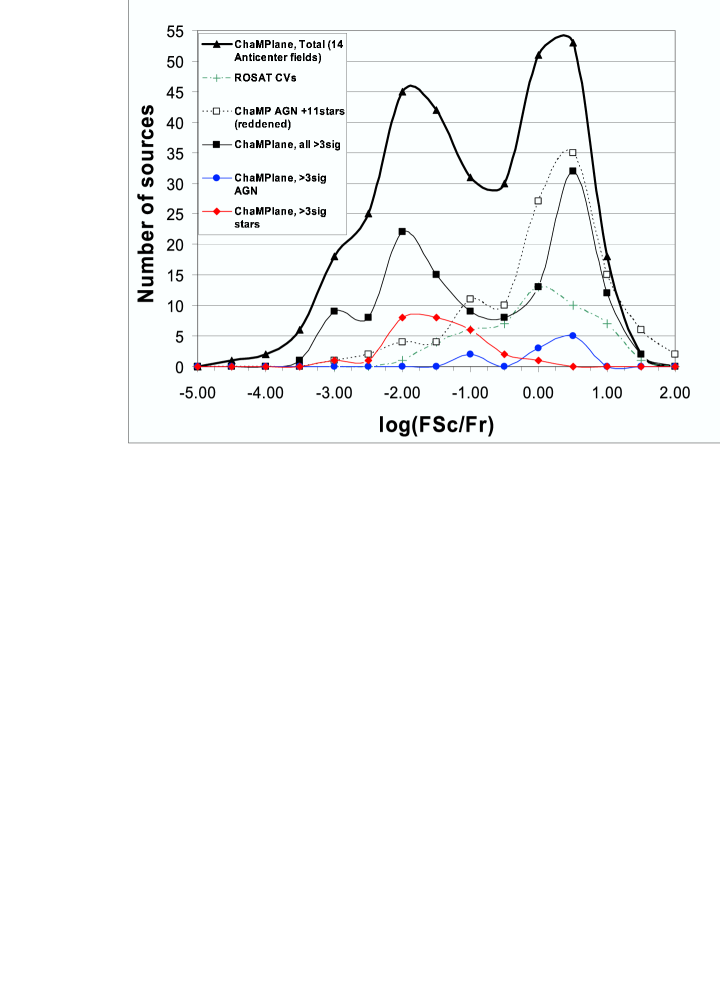
Figure 4.— log(F_X/F_R) distributions (F(Sc) vs. R band) for 324 ChaMPlane Anticenter sources (heavy curve; filled triangles), 131 with well-measured ($\buildrel>\over{\sim}$3$\sigma$) F(Sc) fluxes (solid squares), and their decomposition into 27 spectroscopically confirmed stars (solid diamonds) and 10 AGN (filled circles), with the remainder either unobserved or unclassified due to limited S/N. Comparison distributions are plotted for 49 ROSAT CVs (dot-dashed curve; + symbols) and for 117 ChaMP high latitude survey AGN and stars (short dashed curve; open squares). The ChaMP sources have been reddened to the ChaMPlane field N_H  values (see text). See electronic ApJ for color version.

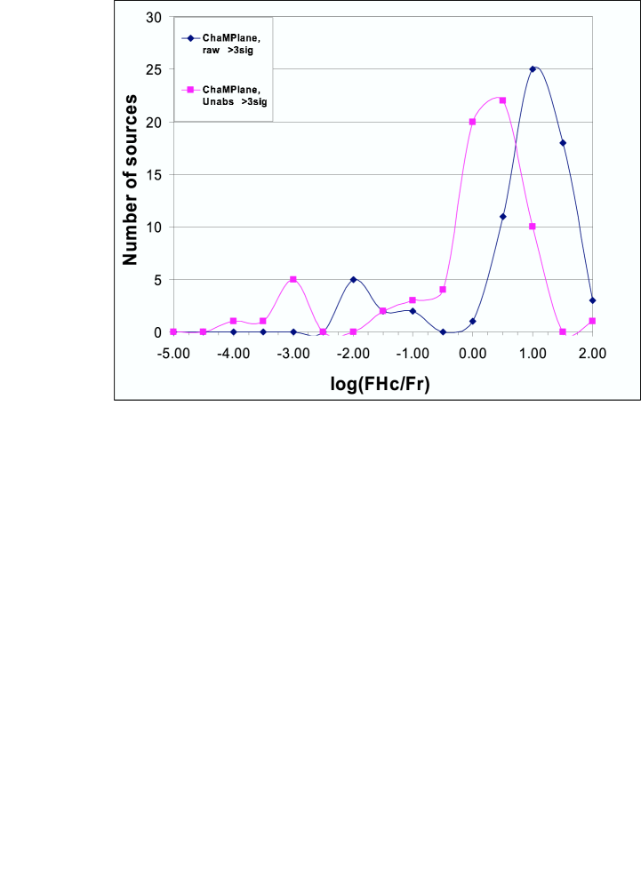
Figure 5.— log(F_X/F_R) distributions (F(Hc) vs. R band) for 68 ChaMPlane Anticenter sources (diamonds) with well determined fluxes in the Hc band. The flux ratios are de-reddened for the full-plane N_H  (an overestimate, generally) in the comparison distribution (squares). Stellar coronal sources are mostly found with log(F_X/F_R) $\buildrel<\over{\sim}$-2 in this band, and are thus better separated from CVs, qLMXBs (and AGN) in the Hc band. See electronic ApJ for color version.

6.2. Constraints on CV Density or Luminosity Function

The apparant lack of bright H$\alpha$  sources among the ChaMPlane Anticenter source IDs allows limits to be derived for the CV space density and/or X-ray luminosity function. We make the conservative assertion that of the 367 sources with optical counterparts, at most $\sim$7 could have (H$\alpha$–R) $\buildrel<\over{\sim}$-0.3 or EW(H$\alpha$) $\buildrel>\over{\sim}$28Å, which allows rejection of dMe stars (see Zhao et al 2005) but not AGN for which emission lines can be redshifted in the H$\alpha$  filter. We include even marginal H$\alpha$  objects (all are $\buildrel>\over{\sim}$1.4–2$\sigma$) for a maximum limit, and without spectroscopic identification (5 were unobserved and 2 had insufficient counts for classification). Since the Sloan Survey CV sample (Szkody et al 2004 and Papers I and II in this series) find 17% of their 99 spectroscopically discovered CVs have EW(H$\alpha$) $\buildrel<\over{\sim}$28Å  our photometric limits for ChaMPlane CVs could be increased by this factor (1.17) to $\buildrel<\over{\sim}$8. Thus a (very) conservative limit from the optically identified ChaMPlane Anticenter sources is that $\buildrel<\over{\sim}$2% are CVs based on these H$\alpha$  limits. The nearly-half of the Anticenter source sample not yet identified optically, with absorbed log(F_X/F_R) $\buildrel>\over{\sim}$1.2 but for which the unabsorbed limit is $\buildrel>\over{\sim}$0, could allow additional CVs, though again the logN-logS results suggest these reddened Anticenter sources are also dominated by AGN.

We now explore whether these limits, from 14 Anticenter fields, provide interesting constraints on the CV number density. Given the current estimates from ROSAT (Schwope et al 2002) and previously Einstein (Hertz et al 1990) that X-ray selected CVs in the solar neighborhood ($\buildrel<\over{\sim}$1 kpc) are detected with space density n_cv $\sim$3 $\times$10^-5 pc^-3 , we derive the numbers expected in each of the 14 fields. Given the estimated distances of the ROSAT CVs, their luminosities in the ROSAT band are peaked at L_x (0.5-2.5keV) $\sim$10³¹ erg s^-1, with only 3 of 49 (Verbunt et al 1997 and Schwope et al 2002) between 10^29-30 erg s^-1. The 22 optically identified CVs detected by Chandra in the deep survey of the globular cluster 47Tuc (Heinke et al 2005) are distributed with a cumulative luminosity function described by either a power law, N($\buildrel>\over{\sim}$F(Sc)) $\propto$ F(Sc)^-0.31±0.04 or a lognormal distribution with mean log(L_x (Sc)) = 31.2$\pm 0.32$. For a “typical” CV spectrum (e.g. a Bremsstrahlung spectrum with kT $\sim$5-10 keV), the L_x (Sc) and L_x (Hc) values are comparable. Thus for L_x (Hc) = 10³⁰ and 10³¹ erg s^-1, we derive (Table 2) the limiting detection distances d₃₀ and d₃₁ for each field using the (maximum) N_H  values for each as derived from Schlegel et al (1998) and given in Table 2. Given the solid angle $\Omega\propto\theta^{2}$ subtended by the full field of the ACIS-I or -S exposure, with $\theta$ = 16$\,{}^{\prime}$ or 8$\,{}^{\prime}$ , respectively (we use the full field, and in this simplified treatment do not allow for the off-axis decline in sensitivity), we then derive the volume in the disk over which CVs could be detected. We assume CVs are distributed in the disk with an exponential z-distribution (Warner 1995) for which we first assume a scale height h = 400pc, or comparable to that recently estimated for LMXBs (Grimm et al 2002). We assume the radial distribution scale in the disk is much larger e.g., $\sim$3.5 kpc, as for stars) and can to first order be ignored in this initial treatment. We then derive the effective detection volume V_eff for each field, using the same formalism adopted by Schwope et al (2002) and Tinney et al (1993). Assuming the CVs are distributed with a z-distribution as n_cv $\propto$ exp^-d(sinb)/h, the effective detection volume out to distance d is

$V_{eff}=\Omega(h/sinb)^{3}(2-(\chi^{2}+2\chi+2)e^{-\chi})$

where $\chi$ = d(sin $b$)/h. We derive this volume for the limiting detection distances d₃₀ and d₃₁ and thus the total number of CVs, N_CVs = n_cv V_eff, given in Table 2 as N₃₀ and N₃₁. Summing over the 14 fields gives a total of 2.3 CVs expected if their characteristic luminosity is L_x = 10³⁰ erg s^-1vs. 53.1 for the L_x = 10³¹ erg s^-1  value. Changing the assumed scale height to 200pc, as assumed by Schwope et al (2002), gives corresponding CV numbers 2.0 - 38.3. Additional limits are given below for a plausible X-ray luminosity function (XLF).

Figure 6.— A_R vs. distance for the 14 Anticenter ChaMPlane fields analyzed in Table 1 using the A_V vs. distance model of Drimmel et al (2003) for each $l,b$ value shown . A_R = 0.75A_V values are plotted after re-scaling the asymptotic N_H  value in the Drimmel model for each field to that given by Schlegel et al (1998). This re-scaled A_R vs. d relation is used to estimate extinction at distances d₃₀ and d₃₁ (see text) for each field.

We then estimate (Table 2) the range of optical R magnitudes these CVs would have for the range of log(F_X/F_V) $\sim$log(F_X/F_R) $\sim$-1 – +1, typical for CVs (Hertz et al 1990, Verbunt et al 1997). However since the optical counterparts for the CVs in some of these Anticenter fields must be appreciably dimmed by the visual extinction, which in R is A_R = 4.2N₂₂, where N₂₂ is the N_H  value in units of 10²² cm^-2as given in Table 2, it is necessary to allow for extinction in the expected R magnitudes as a function of distance through the disk. We do this using the 3D dust model of the Galaxy from Drimmel at al (2003). The Drimmel model computes A_V vs. d, but for these Anticenter fields appears to underestimate the full-plane extinction as indicated by our logN-logS analysis (Hong et al 2005), for which the Schlegel et al (1998) full-plane N_H  gives a better match to the extragalactic source number counts in the unabsorbed Hc band. Thus we re-normalize the Drimmel A_V values by the full-plane N_H  predicted by Schlegel et al and convert to A_R = 0.75A_V for the A_R vs. d plot in Figure 6. This gives A_R for distances d₃₀ and d₃₁ and thus the expected observed range of R magnitudes for CVs for the L_x   and F_X/F_R  ranges given in Table 2.

Finally, we estimate the fraction of the predicted X-ray CVs that should be identified (“easily”) with magnitudes R $\buildrel<\over{\sim}$23 in our ChaMPlane sample. We use the ROSAT distribution of F_X/F_V  as plotted in Fig. 4 (and which we assume to be approximately the same as the F_X/F_R  distribution, given typical CV colors (V-R) $\sim$0.3), to derive the cumulative distribution shown in Figure 7. This gives the fraction of optical CVs vs. R magnitude relative to the R magnitude for log(F_X/F_R) = +1 since these are the faint optical limits, R₃₁ and R₃₀ + 5, as given in Table 2. The cumulative optical identification fractions, C₃₀ and C₃₁, of the X-ray CVs are read off the plot as the fraction value at the “offset magnitude” limits R₃₁ - 23 and (R₃₀ + 5) -23 and given in Table 2. These fractions are then multiplied by the total predicted X-ray CV numbers (CV₃₀ and CV₃₁) to give the predicted number of CVs (ID₃₀ and ID₃₁) that should be optically identified for each field at R $\buildrel<\over{\sim}$23 for these characteristic L_x values.

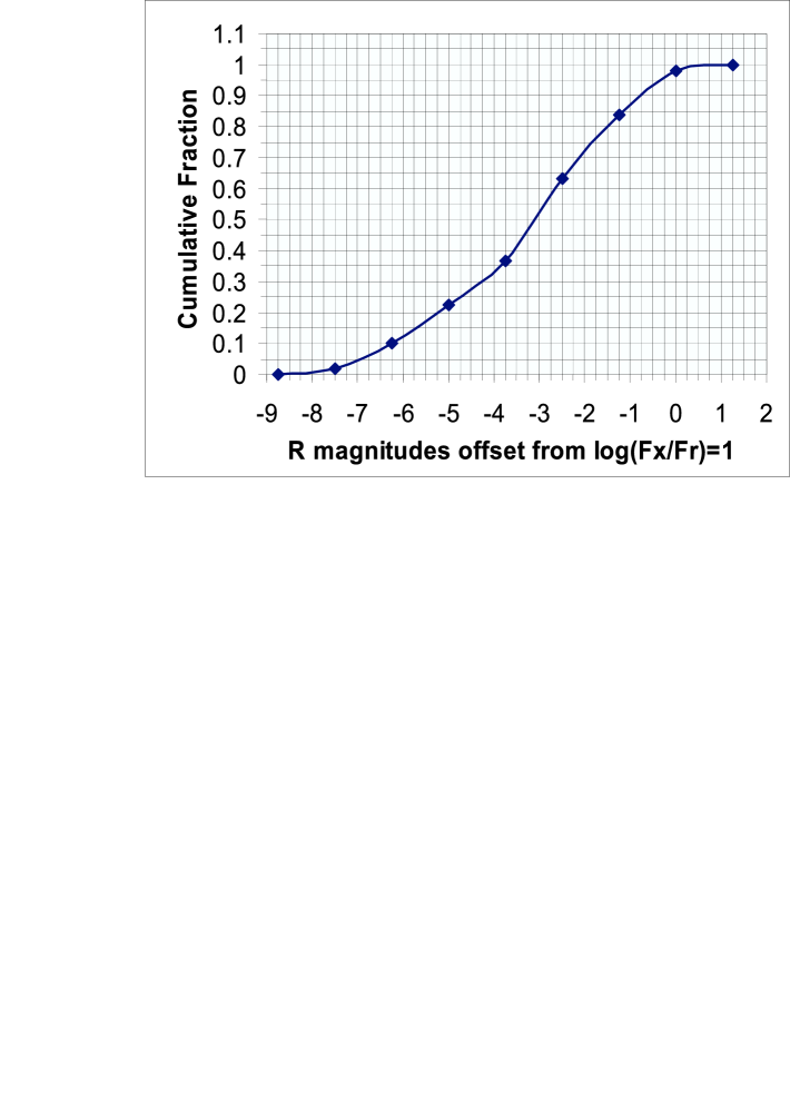
Figure 7.— Cumulative distribution of F_X/F_R  for ROSAT CVs (see text) plotted as a function of R magnitude offset, for a fixed F_X , from the optically faint limit at log(F_X/F_R) = +1 for which the R magnitudes expected for CVs in each field are given in Table 2. The C₃₀ and C₃₁ values in Table 2 are the fractions of CVs expected with R $\buildrel<\over{\sim}$23 for CVs with the corresponding L_x = 10³⁰ and 10³¹ erg s^-1.

7. Conclusions

The X-ray number counts for ChaMPlane sources in the Anticenter (Hong et al 2005) suggest that, as found in a moderately deep Chandra Galactic plane survey of $l,b$ $\sim$28.5^∘,0^∘  as well as ASCA Galactic plane surveys (Ebisawa et al 2003), at fluxes $\buildrel<\over{\sim}$10^-13.5 erg cm^-2 s^-1the AGN and extragalactic source distributions dominate stars and Galactic sources. Although the photometry of an “example” ChaMPlane field, GROJ0422+32 (Zhao et al 2005), shows that most of the 40 optical counterparts (out of 62 sources) in this field have (V-R) and (R-I) colors consistent with their being normal stars, spectroscopy (Rogel et al 2005) of 33 of these counterparts showed that 14 are AGN, 4 are stars and 15 were unidentified (insufficient S/N).

We have conducted preliminary analysis of 14 Anticenter fields to limit their CV content, and contribution from compact binaries generally. Our initial analysis of the ChaMPlane Anticenter CV limits suggests that the local space density of CVs may be overestimated by a factor of $\sim$3 relative to the 3 $\times$  10^-5 pc^-3  value derived for the solar neighborhood from the Einstein and ROSAT surveys. We derive this as follows. The ROSAT CVs are strongly peaked at L_x $\sim$10³¹ erg s^-1, so we first consider the limiting case for this L_x . The much larger volumes in the disk (and halo) that can be reached with Chandra than with ROSAT make it unlikely that the $\sim$38-53 CVs predicted in the 14 fields could be missed if they had local space density n_cv $\sim$3 $\times$10^-5 pc^-3  and X-ray luminosity function with characteristic L_x $\sim$10³¹ erg s^-1. Our conservative upper limit of 8 CVs out of 367 optical IDs could then allow perhaps 14 CVs for the full sample of 631 sources from simple scaling, yielding a deficit factor of $\sim$2.7.

A stronger limit is obtained from the predicted number of CVs which should have magnitudes R $\buildrel<\over{\sim}$23 (“easily” detected in our Mosaic photometry), given our derived F_X/F_R  distribution for ROSAT CVs: for CVs with characteristic L_x $\sim$10³¹ erg s^-1, some 26 CVs should have been optically identified from the ChaMPlane sources. This would suggest a factor of $\sim$3 deficit in CV density. Since it incorporates “known” F_X/F_R  flux ratios for CVs and the extinction vs. distance model (Drimmel et al 2003) for each field, it should be roughly independent of the fraction of ChaMPlane sources optically identified. ChaMPlane sources with R $\buildrel<\over{\sim}$23 are consistent with the F_X/F_R  distributions and extinction for CVs with characteristic L_x $\sim$10³¹ erg s^-1  if n_cv $\sim$1 $\times$  10^-5 pc^-3 .

Allowing for a plausible XLF for disk CVs like that recently derived for CVs in the globular cluster 47 Tuc (Heinke et al 2005), for which we approximate an integral distribution N($\buildrel>\over{\sim}$L_x ) $\propto$L_x ^-0.3 for L_x $\buildrel<\over{\sim}$10^31.5 erg s^-1, steepening to index $\sim$-1.3 for higher luminosities, and assuming a low luminosity cutoff at $\sim$10^29.5 erg s^-1, then $\sim$0.22 of the sources would be detected with L_x $\buildrel>\over{\sim}$10³¹ erg s^-1. This would appear to suggest a reduction by this factor for the CV₃₁ total from that in Table 2, or comparable to our scaled limit of $\buildrel<\over{\sim}$14 CVs. However, the extension of the XLF to larger L_x increases the detection volume and thus CV number predicted. When combined with the addition of the larger number of lower L_x   CVs, a deficit is still indicated. Full consideration of the XLF as well as the the radial scale length of CVs in the galactic disk, e.g. $\sim$3.5kpc as for stars, will be explored in a more detailed analysis with the full ChaMPlane Anticenter sample. Our limits are relatively insensitive to the assumed vertical scale height (h = 200pc vs. 400pc only reduces the expected CV numbers by 28%) and are consistent with the overall CV space density $\sim$10${-5}$ pc^-3  for the solar neighborhood (Patterson 1998).

However the Patterson (1998) estimate is dominated (75%) by short-period CVs below the period gap with low $\dot{m}$ and thus L_x values $\buildrel<\over{\sim}$10³⁰ erg s^-1expected. These can be detected in these ChaMPlane Anticenter fields out to $\sim$1.5 kpc but the numbers expected (CV₃₀ in Table 2) are small. Additional fields in the Anticenter can test this by probing a greater range of $l,b$ values as well as additional regions of low N_H. However the best measurements of the low L_x CV population will likely come from our low-extinction windows (e.g. Baade’s Window) in the Bulge, for which analysis is in progress. Conversely, the luminous (L_x $\sim$10^32-33 erg s^-1) CV distribution may dominate the compact object distributions near the Galactic Center. IR imaging of the sources in the cusp around SgrA* suggests that most are not HMXBs, but are consistent with being luminous CVs (Laycock et al 2005).

With the much larger samples of ChaMPlane data from the full survey (these data represent $\buildrel<\over{\sim}$10% of the total, and cover just 0.6 square degrees), the CV and compact binary (qLMXBs, Be-HMXBs) space density and luminosity functions will be possible to measure or constrain over Galactic scale distances for the first time. The ChaMPlane data and images will be available for easy access and analysis, as described in the Appendix.

Many colleagues have contributed to ChaMPlane. We thank P. Green, D. Kim, J. Silverman and B. Wilkes for early (and continuing) discussions of ChaMPlane vs. ChaMP and D. Kim, especially, for his development of the XPIPE processing script. C. Bailyn, A. Cool, P. Edmonds, M. Garcia and J. McClintock all provided useful input in the early planning stages, and D. Hoard and S. Wachter helped with some early CTIO observations. This work is supported in part by NASA/Chandra grants AR1-2001X, AR2-3002A, AR3-4002A, AR4-5003A and NSF grant AST-0098683. We thank the Chandra X-ray Center for support, and NOAO for support and the Long Term Surveys program.

ChaMPlane Data Archives and VO ANalysis and Display Tools

(see http://hea-www.harvard.edu/ChaMPlane/apj_appendix.html)

We have developed a suite of analysis tools and an on-line database for both the primary ChaMPlane X-ray data (source catalogs) as well as the optical counterpart data. On-line browse access to ChaMPlane observations and data is organized by ObsID (which can also be found on the ChaMPlane website, where all observations can be listed and sorted) and provides a very general and intuitive platform for access to the results. In Appendix Fig. 1 (see http://hea-www.harvard.edu/ChaMPlane/walkthrough_xray.html) we show a screenshot example of access to obsID 676, the field originally observed for the BH transient GROJ0422+32. The left window allows a browse selection of obsID; the middle window enables choice of data return (e.g. formatted text or rdb tables), while the right most windows are: top, the source catalog for the field selected (showing X-ray source ID number, RA, Dec, etc. of the sources in that field); and bottom, the optically identified counterparts for the given source clicked on in the upper window. Following the link at the end of this paragraph of text in the Appendix website leads to a “walk-through” tutorial and demonstration of how to create the composite screen shown in Fig. 1.

In Chandra cycle 5, we developed and released a Virtual Observatory (VO) node to facilitate access and on-line analysis of ChaMPlane data. Database access is via the VO interface in the image display and analysis package ds9, which is a major upgrade from the original SAOimage package and allows many new features, including VO. In general, the user connects through the ds9 toolbar or via any web browser (http://hea-www.harvard.edu/ChaMPlane/data/archive). Upon connection the ChaMPlane toolbar is automatically installed on the user’s own ds9 running locally on the user’s machine. Commands and results are exchanged between the user’s machine and the ChaMPlane data server at CfA running search and analysis scripts. This setup has the considerable advantage of adding custom tools and data to an already familiar platform, while maintaining the data archive and analysis and display tools at a central facility for maintenance and upgrades. A demonstration and link to a “walk-through” of this ChaMPlane VO facility is given in the following paragraph.

The ChaMPlane VO provides access to our deep Mosaic optical (V, R, I, H$\alpha$) images, catalogs of their optical photometry, Chandra images with exposure-map correction, X-ray source data and details of X-ray sources with identified optical counterparts. Images, datatables and plots (e.g. color-magnitude diagrams) can be generated for sources detected in any desired region on the Chandra or Mosaic images. Data can be selected by defining regions with a cursor to overlay X-ray or optical source positions selected for a given characteristic on either the ACIS or Mosaic field of view. An example is shown in Appendix Fig. 2 from the source selection shown in Appendix Fig. 1. Once again, following the link which is on the website Appendix just after Fig. 2 leads to a “walk-through” tutorial and demonstration of how to create the composite screen shown in web appendix Fig. 2. We note that as a matter of scientific interest, the two Chandra sources identified as H$\alpha$  objects in web appendix Fig. 2 – namely, the two sources with red (H$\alpha$  object) source circles and optical source ID numbers overplotted in Fig. 2 on both the optical Mosaic image (image on left) and the smoothed Chandra image (image on right), are identified from WIYN spectroscopy (Rogel et al 2005) as a dMe star (optical ID 111135) and a QSO at z = 1.31 (optical ID 111329), with the (red) wing of MgII at $\lambda$2802 redshifted into the H$\alpha$  filter! Additional ChaMPlane VO tools for interactive inspection of both the X-ray and optical data are described on a separate link (http://hea-www.harvard.edu/ChaMPlane/walkthrough_ds9.html) at the very end of the web appendix and via the Data Archive/Virtual Observatory link on the ChaMPlane homepage.

X-ray and optical data are now available on line for the initial 14 fields in the Anticenter. X-ray and optical images and source catalogs for a given field or region of the survey will be added to the database when the first corresponding analysis papers are submitted for publication. Calibrated V, R, I, H$\alpha$  Mosaic images and photometry are submitted in parallel to the NOAO Long Term Survey archives and CDS; these have already been archived at NOAO for the initial 14 Anticenter fields.

References

- (1) Agol, E. and Kamionkowski, M. 2002, MNRAS, 334, 553
- (2) Brandt, W.N. and Hasinger, G.R. 2005, ARAA, 43 in press (astro-ph/0503009)
- (3) Drimmel, R., Cabrera-Lavers, A. and Lopez-Corredoira, M. 2003, A&A, 409, 205
- (4) Ebisawa, K. et al 2003, AN, 324, 52
- (5) Green, P. et al 2004, ApJS, 150, 43
- (6) Grimm, H.J., Gilfanov, M. and Sunyeaev, R. 2002, A&A, 391, 923
- (7) Grindlay, J.E. 1985, in IAU 113, Dynamics of Star Clusters, ed. J. Goodman & P. Hut (Dordrecht-Kluwer), 43
- (8) Grindlay, J.E. et al 2003, AN, 324, 57
- (9) Heinke, C., Grindlay, J.E. et al 2005, ApJ, 625, 796
- (10) Heise, J., 1998 in Active X-ray Sky (Elsevier: Amsterdam), 186
- (11) Hertz, P. and Grindlay, J. 1984, ApJ, 278, 137
- (12) Hertz, P., Bailyn, C.D., Grindlay, J.E. et al 1990, ApJ, 364, 251
- (13) Hong, J., Schlegel, E.M. and Grindlay, J.E. 2004, ApJ, 614, 508
- (14) Hong, J. et al 2005 ApJ, in press
- (15) Kim, D.W. et al 2004, ApJ, 600, 59
- (16) Laycock, S. et al 2005, ApJ, submitted
- (17) Motch, C. et al 2003, AN, 324, 61
- (18) Muno, M.P. et al 2003, ApJ, 589, 225
- (19) Patterson, J. 1998, PASP, 110, 1132
- (20) Perna, R. et al 2003, ApJ, 594. 936
- (21) Rogel, A. et al 2005, ApJ, submitted
- (22) Schlegel, D., Finkbeiner, D. and Davis, M. 1998, ApJ, 500, 525
- (23) Schwope, A.D. et al 2002, A&A, 396, 895
- (24) Schmitt, J. et al 2004, A&A, 417, 651
- (25) Szkody, P. et al 2004, AJ, 128, 1882
- (26) Tanaka, Y. & Lewin, W.H.G. 1995, in X-Ray Binaries, 126
- (27) Tinney, C.G., Reid, I.N. and Mould, J.R. 1993, ApJ, 414, 254
- (28) Townsley, D.M. and Bildsten, L. 2005, ApJ, 628, 395
- (29) van Paradijs, J. and McClintock, J.E. 1995, in X-ray Binaries, W. Lewin, J. van Paradijs and E. van den Heuvel, eds., Cambridge Univ. Press, p. 60
- (30) Verbunt, F., Bunk, W.H., Ritter, E. & Pfefferman, E. 1997, A&A, 327, 602
- (31) Voges, W., Aschenbach, B., Boller, Th. et al 1999, A&A, 349, 389
- (32) Wang, Q.D. et al 2002, Nature, 415, 148
- (33) Warner, B. 1995, Cataclysmic Variables, Camb. Press
- (34) Yi, I. and Grindlay, J.E. 1998, ApJ, 505, 828
- (35) Zhao, P. et al. 2003, AN, 324, 176
- (36) Zhao, P. et al 2005, ApJS, in press