Giant Molecular Clouds are More Concentrated to Spiral Arms than Smaller Clouds

Abstract

From our catalog of Milky Way molecular clouds, created using a temperature thresholding algorithm on the Bell Laboratories ${}^{13}\mathrm{CO}$ Survey, we have extracted two subsets: (1) Giant Molecular Clouds (GMCs), clouds that are definitely larger than $10^{5}\,\mathrm{M_{\odot}}$, even if they are at their “near distance”, and (2) clouds that are definitely smaller than $10^{5}\,\mathrm{M_{\odot}}$, even if they are at their “far distance”. The positions and velocities of these clouds are compared to the loci of spiral arms in $\ell,\,v$ space. The velocity separation of each cloud from the nearest spiral arm is introduced as a “concentration statistic”. Almost all of the GMCs are found near spiral arms. The density of smaller clouds is enhanced near spiral arms, but some clouds ($\sim\,10\%$) are unassociated with any spiral arm. The median velocity separation between a GMC and the nearest spiral arm is $3.4\pm 0.6\,{\mathrm{km\,s^{-1}}}$, whereas the median separation between smaller clouds and the nearest spiral arm is $5.5\pm 0.2\,{\mathrm{km\,s^{-1}}}$.

1 Introduction

The Galaxy as a whole affects star formation through the mechanism of spiral structure. Stars in galactic disks tend to develop spiral-shaped density waves that arise either through spontaneous instability or through gravitational perturbations from nearby galaxies or a central bar. The spiral density wave modulates the gravitational potential in the disk, and the interstellar medium reacts non-linearly to this varying potential, gathering and concentrating the gas. Giant Molecular Clouds (GMCs) form, leading to a local increase in the star formation rate and the creation of giant $\mathrm{H\,\scriptstyle II}$ regions. The cloud formation process is not well understood, and is the subject of ongoing investigation (Elmegreen, 2000; Pringle et al., 2001; Hartmann et al., 2001; Zhang et al., 2002; Elmegreen, 2002; Ostriker & Kim, 2004).

In this Letter, we measure the degree to which GMCs and smaller molecular clouds are concentrated in the spiral arms of the Milky Way, to provide a quantitative comparison with theoretical models of molecular cloud formation. In §2, we take the Bell Laboratories ${}^{13}\mathrm{CO}$ Survey data (Lee et al., 2001) and use a brightness temperature thresholding algorithm to create a catalog of molecular clouds. From this catalog, we extract a set of clouds that are definitely GMCs, and a set of clouds that are definitely smaller than GMCs. In §3, we use surveys of neutral and ionized hydrogen to define the spiral arms. In §4, we compare the locations of clouds in $(\ell,\,v)$-space with the spiral arm loci. We show that the GMCs and the smaller clouds have significantly different distributions. The GMCs are more concentrated to the spiral arms than the smaller clouds.

2 Cloud Identification and Mass Estimation

A catalog of clouds was generated from the Bell Laboratories ${}^{13}\mathrm{CO}$ survey data (Lee et al., 2001) using a thresholding technique described in Stark & Lee (2005). This survey contains $2.3\,\times\,10^{7}$ pixels of ${}^{13}\mathrm{CO}$ data, each $0.05{{}^{\circ}}\,\times\,0.05{{}^{\circ}}\,\times\,0.68\,{\mathrm{km\,s^{-1}}}$ in size. Survey pixels having $T_{R}^{*}>T_{\mathrm{th}}$ are identified and grouped together in $(\ell,\,b,\,v)$ space to make a “cloud”, where all the pixels constituting the cloud are above the threshold and also adjacent to at least one other pixel that is also above the threshold. A “cloud” is then a connected volume of pixels, all of which are above the threshold. Applying the thresholding method with $T_{\mathrm{th}}=1\mathrm{K}$ on the Bell Laboratories ${}^{13}\mathrm{CO}$ Survey yields a catalog of 1,400 clouds. As further described in Stark & Lee (2005), we assign several possible distances to each cloud based on our knowledge of the velocity field of the Galaxy. Essentially, the distances correspond to the “near” and “far” points of the distance ambiguity (cf. Mihalas 1968), plus some additional uncertainty due to random motions. Each cloud has a range of possible distances.

We want to distinguish GMCs from smaller clouds, but the distances are uncertain, and so are the luminosities and estimated masses. We can, however, derive a subset of the catalog that contains only GMCs, and another subset that that contains only clouds that are definitely smaller than a GMC. For the purposes of this Letter, we define a GMC as a member of our catalog with $L(^{13}\mathrm{CO})\,>\,5\times 10^{3}\,\mathrm{K\,km\,s^{-1}\,pc^{2}}$. The mass corresponding to this luminosity is $1\times 10^{5}\,\mathrm{\mathrm{M_{\odot}}}$, based on the mass-luminosity relation $M_{c}=[20\,\mathrm{\mathrm{M_{\odot}}/K\,km\,s^{-1}\,pc^{2}}]L(^{13}\mathrm{CO})$ derived in Stark & Lee (2005) for clouds identified by the method we use here. For each cloud in the catalog, we calculate the range of luminosities corresponding to the range of possible distances. If all these possible luminosities exceed the luminosity threshold $L(^{13}\mathrm{CO})\,>\,5\times 10^{3}\,\mathrm{K\,km\,s^{-1}\,pc^{2}}$, the cloud is definitely a GMC, regardless of the distance uncertainties. Applying this criterion to the catalog yields 56 GMCs. If all the possible luminosities fall below the threshold, the cloud is definitely not a GMC, and the cloud is included in the “definite small cloud” set. This second criterion yields 1257 small clouds. Our catalog also contains 87 clouds that do not fulfill either criterion. These are moderately-large clouds whose distance is not well determined, and we exclude them from further consideration.

3 Spiral Arm Loci

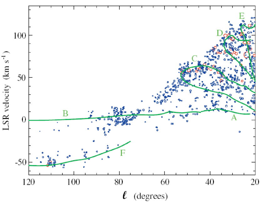
Figure 1: Distribution in $\ell$ and $v$ of two sets of clouds selected from the Bell Laboratories ${}^{13}\mathrm{CO}$ Survey. The area of each symbol is proportional to the velocity width of the corresponding cloud. The red clouds have a mass $>\,10^{5}\,\mathrm{M_{\odot}}$, even if they are at their near distance; the blue clouds have a mass $<\,10^{5}\,\mathrm{M_{\odot}}$, even if they are at their far distance. The green curves indicate the loci of spiral arms: A and B are the local arm, C is the Sagittarius arm, D is the Scutum arm, E is the 3 kpc arm, and F is the Perseus arm.

Spiral arms in the Milky Way have been identified in surveys of 21 cm atomic hydrogen and radio recombination lines. Here we adopt the analyses of Reifenstein et al. (1970), Burton & Shane (1970), Shane (1972), Lindblad et al. (1973), and Simonson (1976), to determine the locations of the spiral arms in $(\ell,\,v)$ space: we take locations defining the spiral arms from these references, and interpolate using cubic spline functions. The loci of the arms are well-determined for $20{{}^{\circ}}\,<\,\ell\,<\,140{{}^{\circ}}$, but not for the Galactic Center Region. We therefore exclude from further analysis all clouds with $\ell<20{{}^{\circ}}$. This reduces the samples to 39 GMCs and 932 smaller clouds. The locations of the clouds, and the locations of the spiral arms, are plotted in figure 1. The spiral arms are identified by letters, as in Cohen et al. (1980).

Drawing the spiral arms onto the $(\ell,\,v)$ diagram of the Milky Way has been controversial. The criteria adopted by the above authors for the placement of the arms are subjective and ill-defined. Arms “A” and “B”, the local arm and the Lindblad Ring, are not large-scale features of the Galaxy, but local spurs that loom large because they are close to the Sun. Spiral arms “A” through “F” are adopted here because they are traditional and because there is no alternative; the analysis below will, however, be seen to support this initial choice.

Almost all the GMCs (red circles) lie close to spiral arms. The most notable exceptions are the GMCs in the bridge between the Sagittarius (C) and Scutum (D) arms near $\ell=38{{}^{\circ}}$, $v=90\,{\mathrm{km\,s^{-1}}}$. The local spiral arm and Lindblad Ring (A and B) contain no GMCs within the area of sky covered by the Bell Labs survey. As noted by Cohen et al. (1980), the Perseus arm (F) is particularly distinct and well-separated from surrounding material.

4 Concentration of Clouds to the Arms

There is at least one spiral arm at some velocity for each value of $\ell$ in figure 1. We can therefore define a “concentration statistic” for each cloud: the absolute value of the separation in velocity between that cloud and the nearest spiral arm, $|{\Delta v}|$. The set of $|{\Delta v}|$ for each of our cloud samples is the distribution of separations of those clouds from the spiral arm loci. These distributions are plotted in figure 2 for the GMC and small cloud samples. The small cloud distribution has a long tail, containing about 10% of all clouds, that extends to large values of $|{\Delta v}|$. Most of these are near $\ell\,\approx\,55{{}^{\circ}},\,v\,\approx\,30\,{\mathrm{km\,s^{-1}}}$, where we have a long line of sight that falls between spiral arms and includes the tangent velocity, where the phase space density is high. These are clear examples of interarm clouds. All but five of the GMCs have $|{\Delta v}|\,<\,14\,{\mathrm{km\,s^{-1}}}$. Of those five, four are clouds in the Sagittarius-Scutum bridge (Cohen et al., 1980).

The Kolmogorov-Smirnov statistic (Press et al., 1992) is the largest vertical separation between the two distributions, as shown in figure 2. The hypothesis that the two sets of $|{\Delta v}|$ are drawn from the same parent distribution is rejected at the 94% level by the Kolmogorov-Smirnov test — it is highly likely that the GMCs are distributed differently with respect to the spiral arms than are the small clouds. The two distributions have significantly different medians. The median $|{\Delta v}|$ for the GMCs is $3.4\pm 0.6\,{\mathrm{km\,s^{-1}}}$, whereas the median $|{\Delta v}|$ for the small clouds is $5.5\pm 0.2\,{\mathrm{km\,s^{-1}}}$. The errors in the medians are estimated by the bootstrap method (Efron & Gong, 1983).

We will compare these results with the concentration statistics of objects that have the same radial distribution and velocity dispersion as molecular clouds but are azimuthally symmetric, and therefore have no concentration to spiral arms. The radial distribution can be parameterized by:

$$\rho\,\propto\,R^{\alpha}\,\mathrm{exp}\left(-{{R}\over{R_{\mathrm{s}}}}\right)\,,$$ (1)

where $\rho$ is the surface density of objects, $R$ is radius from the galactic center, and $\alpha$ and $R_{\mathrm{s}}$ are parameters. The galactic rotation curve is taken to be flat, at a velocity $\Theta_{0}$. The velocity dispersion is Gaussian, with a one-dimensional root-mean-square of $\sigma_{v}$ (e.g., Stark & Brand, 1989). A set of Monte Carlo objects were generated by the following steps: (1) Choose a set of parameters, $\alpha$, $R_{\mathrm{s}}$, $\Theta_{0}$ and $\sigma_{v}$. (2) Use a random number generator to create a set of objects in two dimensions that have a radial distribution given by equation 1. (3) Calculate the $\ell$ and $v$ of each object as seen from the Sun at $\mathrm{R_{\odot}}=8\,\mathrm{kpc}$. (4) Generate a random Gaussian deviate for each object from a distribution with $\sigma\,=\,\sigma_{v}$ and zero mean, and add it to each $v$. (5) Compare the resulting set of random $(\ell,v)$ values to the catalog of actual molecular clouds, using a two-dimensional Kolmogorov-Smirnov test (Press et al., 1992). (6) Go back to step 1, varying parameters to maximize the similarity between the random set of objects and the observed catalog.

This procedure results in the parameters $\Theta_{0}\,=\,215\,{\mathrm{km\,s^{-1}}}$, $R_{\mathrm{s}}\,=\,1.7\,\mathrm{kpc}$, $\alpha=2.3$, and $\sigma_{v}\,=\,7.7\,{\mathrm{km\,s^{-1}}}$. This value of $\Theta_{0}$ should not be taken to be a measure of the Sun’s rotational velocity. If the rotation curve were parameterized as $\Theta(R)\,\approx\,\Theta_{0}\,+\,(R/\mathrm{R_{\odot}})\Theta_{1}\,+\,\ldots\,$, then $\Theta_{1}$ cannot be constrained by fitting to objects in the inner Galaxy: galactic kinematics looks the same with a solid-body term added to the rotation curve. These data do not constrain $\alpha$ very well either, since our cutoff at $\ell\,=\,20{{}^{\circ}}$ eliminates much of the molecular hole at $R\,\approx\,3.5\,\mathrm{kpc}$. The shape of the inner edge of this hole is parameterized by $\alpha$, and almost all values of $\alpha$ between 2 and 3 fit well. The quick drop-off of the molecular ring to larger radii, $R_{\mathrm{s}}\,=\,1.7\,\mathrm{kpc}$, is typical of fits to first quadrant molecular line surveys (Burton & Gordon, 1978; Solomon et al., 1979). The value of $\sigma_{v}\,=\,7.7\,{\mathrm{km\,s^{-1}}}$ is consistent with the value $\sigma_{v}\,=\,7.8^{+0.6}_{-0.5}\,{\mathrm{km\,s^{-1}}}$ determined for moderately-large clouds near the Sun by Stark & Brand (1989).

The distribution of $|{\Delta v}|$ values for the Monte Carlo objects is plotted in green in figure 2, and their median value of $|\Delta v|$ is $7.81\pm 0.05\,{\mathrm{km\,s^{-1}}}$. This value is robust, in the sense that essentially any azimuthally-symmetric distribution of random objects in the galactic plane that we have tried will produce a median value of $|\Delta v|$ that is greater than $7\,{\mathrm{km\,s^{-1}}}$. The small molecular clouds are more concentrated to spiral arms than random objects, and the GMCs are even more concentrated than the small clouds.

5 Discussion

It is unfortunate that we cannot observe the Milky Way from the outside, and see the spatial relationship between the molecular clouds and the spiral arms directly. Interferometric observations of CO in other galaxies having well-defined spiral structure shows that the CO emission is concentrated to the spiral arms (Murgia et al., 2005). In the Milky Way, most of the CO emission is from GMCs. This is illustrated in figure 3. Here we have taken the catalog subset discussed in Stark & Lee (2005), where the clouds were selected to have well-determined distances, and further restricted that subset to clouds with $\ell\,>\,20{{}^{\circ}}$. Figure 3 shows the distribution of virial masses for these clouds. The vast majority of the CO-emitting material, over 85%, is in the GMCs. Since the CO luminosity per molecule is approximately constant (Liszt, 1984), the majority of the CO luminosity will also arise in GMCs. It seems likely that this is true of all spiral galaxies, and that the concentration of CO to spiral arms is principally a concentration of GMCs to the spiral arms.

Given the median velocity separations derived in §4, we can estimate the typical size of the spatial deviations from the spiral arms. The distributions of $\Delta v$ values are approximately Gaussian for small values, ignoring the long tails. For purposes of this estimate, we assume that the spatial deviations from the arms are also Gaussian. Let $\sigma_{a}^{2}$ be the Gaussian velocity variance; its square root is proportional to the observed median, $m$:

$$2\int_{0}^{m}\,{{1}\over{\sigma_{a}\,\sqrt{2\pi}}}\,\mathrm{e}^{-{{v^{2}}\over{2\,\sigma_{a}^{2}}}}\,\mathrm{d}v\,=\,\mathrm{erf}\left({{m}\over{\sqrt{2}\,\sigma_{a}}}\right)\,=\,{{1}\over{2}}\,,$$ (2)

or $\sigma_{a}=m/(b\sqrt{2})=1.48\,m$, where $\mathrm{erf}(b)\,\equiv\,{{1}\over{2}}$. So $\sigma_{a}\,\approx\,8.2\,{\mathrm{km\,s^{-1}}}$ for the small clouds and $\sigma_{a}\,\approx\,5.0\,{\mathrm{km\,s^{-1}}}$ for the GMCs. We know that the one-dimensional root-mean-square velocity dispersions of clouds are $\sigma_{v}\,\approx\,7.8\,{\mathrm{km\,s^{-1}}}$ for moderate-sized clouds ($M\,\mathrel{\raise 1.50696pt\hbox{$\scriptstyle<$}\kern-6.00006pt\lower 1.72218pt\hbox{{$\scriptstyle\sim$}}}\,10^{5}\,\mathrm{M_{\odot}}$, Stark & Brand 1989) and $\sigma_{v}\,\approx\,4\,{\mathrm{km\,s^{-1}}}$ for GMCs ($M\,>\,10^{5.5}\,\mathrm{M_{\odot}}$, Stark & Lee 2005). This dispersion will, approximately, add in quadrature with the amount of velocity separation caused by the spatial deviations and the rotation curve, $\sigma_{r}$:

$$\sigma_{a}^{2}\,\approx\,\sigma_{v}^{2}+\sigma_{r}^{2}\,.$$ (3)

A typical spatial deviation of the clouds from the spiral arm is then

$$\Delta r\,\sim\,{{\sigma_{r}}\over{|{{\mathrm{d}v}\over{\mathrm{d}r}}|}}\,\approx\,{{\sqrt{\sigma_{a}^{2}-\sigma_{v}^{2}}}\over{|{{\mathrm{d}v}\over{\mathrm{d}r}}|}}\,\sim\,50\,\mathrm{pc},$$ (4)

where ${|{{\mathrm{d}v}\over{\mathrm{d}r}}|}\,\sim\,50\,{\mathrm{km\,s^{-1}}}\,\mathrm{kpc}^{-1}$ is a typical change in radial velocity with distance due to galactic rotation. The estimated separation, $\Delta r\,\sim\,50\,\mathrm{pc}$, which applies to both the small clouds and the GMCs, is small compared to the scale of a spiral arm. We do not want to make too much of this rough estimate, but we can say that aside from the long tail in the distribution of $\Delta v$ values, the data are consistent with the hypothesis that the spatial concentration of most molecular clouds to the spiral arms is high.

The complete picture of the interaction of molecular clouds with spiral arms is a dynamical process in six-dimensional phase space. The Bell Laboratories ${}^{13}\mathrm{CO}$ Survey provides statistical information about two spatial and one velocity dimension. We have seen in Stark & Lee (2005) that, on average, the GMCs are tightly concentrated to the galactic plane, with a FWHM scaleheight about 30 pc. We now see that these same GMCs are concentrated to the spiral arms as well. Most clouds are associated with spiral arms, aside from the outliers that are examples of interarm clouds. Among clouds near the arms, the GMCs are significantly more concentrated to the arms in velocity than are the small clouds.

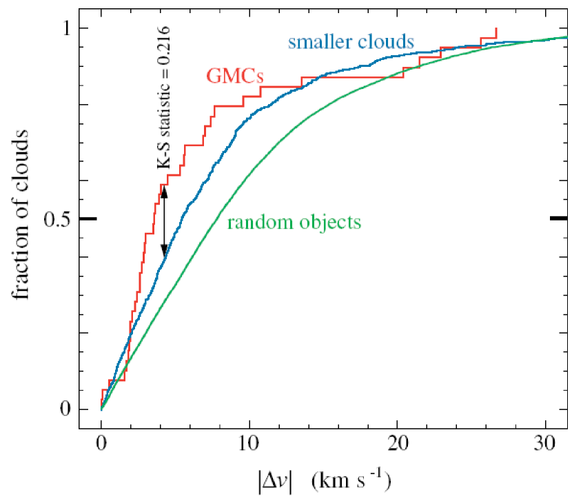
Figure 2: Cumulative distribution of separation velocities from the nearest spiral arm. For each cloud in figure 1, the velocity separation, $|\Delta v|$, from the nearest spiral arm is determined. The two distributions of these velocities for 39 GMCs and for 932 smaller clouds are plotted here. The ordinate is the fraction of clouds of each size having a separation velocity less than the value on the abscissa. The value of the Kolmogorov-Smirnov statistic is shown. The green line is the distribution of separation velocities for a set of azimuthally-symmetric random objects that have the same radial distribution as the molecular clouds.

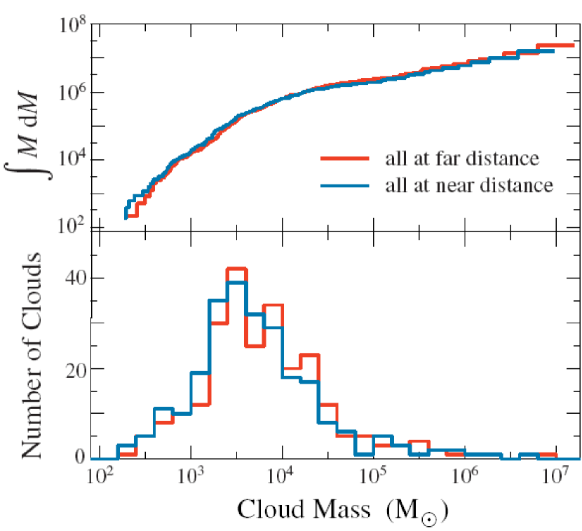
Figure 3: Distribution of estimated virial masses of a cloud sample from the Bell Laboratories ${}^{13}\mathrm{CO}$ Survey. This subset of clouds was selected to have small distance uncertainty in Stark & Lee (2005). The red curves show the distribution if all the clouds are at their far distance, and the blue curves show the distribution if all the clouds are at their near distance. The lower panel shows a histogram of the cloud mass distribution in logarithmic bins. The coarse sampling grid of the survey may cause it to miss some clouds smaller than $\sim\,10^{3}\,\mathrm{M_{\odot}}$. The upper panel shows the integrated mass distribution. Over 85% of the total mass is in GMCs ($M\,>\,10^{5}\,\mathrm{M_{\odot}}$).

References

- Burton & Gordon (1978) Burton, W. B. & Gordon, M. A. 1978, A&A, 63, 7
- Burton & Shane (1970) Burton, W. B. & Shane, W. W. 1970, in IAU Symp. 38: The Spiral Structure of our Galaxy, 397
- Cohen et al. (1980) Cohen, R. S., Cong, H., Dame, T. M., & Thaddeus, P. 1980, ApJ, 239, L53
- Efron & Gong (1983) Efron, B. & Gong, G. 1983, The American Statistician, 37, 36
- Elmegreen (2000) Elmegreen, B. G. 2000, ApJ, 530, 277
- Elmegreen (2002) —. 2002, ApJ, 577, 206
- Hartmann et al. (2001) Hartmann, L., Ballesteros-Paredes, J., & Bergin, E. A. 2001, ApJ, 562, 852
- Lee et al. (2001) Lee, Y., Stark, A. A., Kim, H.-G., & Moon, D.-S. 2001, ApJS, 136, 137
- Lindblad et al. (1973) Lindblad, P. O., Grape, K., Sandqvist, A., & Schober, J. 1973, A&A, 24, 309
- Liszt (1984) Liszt, H. S. 1984, Comments on Astrophysics, 10, 137
- Mihalas (1968) Mihalas, D. 1968, Galactic Astronomy (W. H. Freeman and Company)
- Murgia et al. (2005) Murgia, M., Helfer, T. T., Ekers, R., Blitz, L., Moscadelli, L., Wong, T., & Paladino, R. 2005, A&A, 437, 389
- Ostriker & Kim (2004) Ostriker, E. C. & Kim, W.-T. 2004, in ASP Conf. Ser. 317: Milky Way Surveys: The Structure and Evolution of our Galaxy, 248
- Press et al. (1992) Press, W. H., Teukolsky, S. A., Vetterling, W. T., & Flannery, B. P. 1992, Numerical Recipies in C (Cambridge University Press)
- Pringle et al. (2001) Pringle, J. E., Allen, R. J., & Lubow, S. H. 2001, MNRAS, 327, 663
- Reifenstein et al. (1970) Reifenstein, E. C., Wilson, T. L., Burke, B. F., Mezger, P. G., & Altenhoff, W. J. 1970, A&A, 4, 357
- Shane (1972) Shane, W. W. 1972, A&A, 16, 118
- Simonson (1976) Simonson, S. C. 1976, A&A, 46, 261
- Solomon et al. (1979) Solomon, P. M., Sanders, D. B., & Scoville, N. Z. 1979, ApJ, 232
- Stark & Brand (1989) Stark, A. A. & Brand, J. 1989, ApJ, 339, 763
- Stark & Lee (2005) Stark, A. A. & Lee, Y. 2005, ApJ, 619, L159
- Zhang et al. (2002) Zhang, T., Song, G., Yang, Z., Chen, L., Zhang, B., Li, N., & Cui, J. 2002, Chinese Astronomy and Astrophysics, 26, 276