A differential rotation driven dynamo in a stably stratified star

We present numerical simulations of a self-sustaining magnetic field in a differentially rotating non-convective stellar interior. A weak initial field is wound up by the differential rotation; the resulting azimuthal field becomes unstable and produces a new meridional field component, which is then wound up anew, thus completing the ‘dynamo loop’. This effect is observed both with and without a stable stratification. A self-sustained field is actually obtained more easily in the presence of a stable stratification. The results confirm the analytical expectations of the role of Tayler instability.

1 Introduction

It has long been known that magnetic fields can be generated by a dynamo operating in the convective zone of a differentially rotating star (e.g. Parker (1979)). A toroidal field is produced by winding-up of the poloidal (meridional) component, and the bubbles of gas moving upwards and downwards move perpendicular to these toroidal field lines, bending them and creating a new poloidal component, closing the ‘dynamo loop’. This type of dynamo has been the subject of extensive work over several decades. A process like this has been held responsible for the magnetism of stars with convective envelopes like the Sun.

Whether or not such direct causation by convection is actually the correct explanation of dynamos like the solar cycle, the predominance of this view has obscured the fact that self-sustained magnetic fields do not require the presence of convection or other imposed small scale velocity fields. A magnetic field can produce small-scale perturbations from its own instability, without recourse to externally imposed perturbations. A well-known example in the context of accretion discs, where a dynamo was produced when differential rotation wound up a field which was then subject to magnetohydrodynamic instability (Hawley et al. 1996).

The same principle was applied by Spruit (2002) to differentially rotating stars. In this scenario, a toroidal field is wound up by differential rotation from a weak seed field. The field remains predominantly toroidal, subject to decay by instability of the field, but is continuously regenerated by the winding-up of irregularities produced by the instability. This scenario has been applied in stellar evolution calculations of the internal rotation of massive stars by Heger et al. (2003) and Maeder & Meynet (2003). The process is conceptually similar to the small-scale self-sustained fields found in MHD simulations of accretion discs, but operates on a different form of MHD instability (pinch-type or Tayler instability as opposed to magnetorotational, cf. Spruit 1999).

A self-sustained field of this type could have important implications for not only the magnetism of a star, but also for the transfer of angular momentum. Differential rotation is created, when the star is formed, as a consequence of conservation of angular momentum when parts of it contract or expand, and through angular momentum loss through a stellar wind (‘magnetic braking’). In the absence of a magnetic field, kinetic viscosity would eventually damp differential rotation, but only on a time-scale much longer than the lifetime of the star. If a weak magnetic field were present in a star with infinite conductivity, the field would be wound up, its Lorentz force exerting a force back on the gas, tending to slow the differential rotation. If we assume that no magnetohydrodynamic instabilities were present, the energy of the field would become eventually comparable to the kinetic energy of the differential rotation, and the field would exert a force on the gas strong enough to reverse the differential rotation. Oscillations would follow, with energy continuously being transferred from kinetic to magnetic and back again (Mestel (1953)). Finite conductivity would have the effect of damping these oscillations. However, if the magnetic field became unstable, as we expect it to, the energy of the field need never reach a level comparable to the kinetic energy and the direction of differential rotation would never be reversed. Instead, differential rotation would gradually be slowed, and the magnetic field held at a low steady-state level. This could be what has happened in the radiative core of the Sun, explaining the near-uniform rotation there (Schou et al. (1998), Charbonneau et al. (1999)).

While such a dynamo process is plausible, it has so far been described only in terms of an elementary scaling model (Spruit 2002). With the calculations presented here we verify, first of all, the existence of a self-sustained field generation process. At the next level, the goal is to compare the properties of the numerical results with the predictions of the model, in particular concerning the central role of Tayler instability. The field strength resulting from the dynamo process depends on the balance between the decay of the toroidal field and the winding up of irregularities. The analytic model only presents the basic scaling of this balance with parameters like the strength of the differential rotation; the actual values of the coefficients in this scaling have to be found by numerical simulations.

1.1 Instability of a toroidal field

Tayler (1973) and Acheson (1978) looked at toroidal fields in stars, that is, fields that have only an azimuthal component $B_{\phi}$ in a cylindrical coordinate frame $(\varpi,\phi,z)$ with the origin at the centre of the star. With the energy method, Tayler derived necessary and sufficient stability conditions in adiabatic conditions (no viscosity, thermal diffusion or magnetic diffusion). The main conclusion was that such purely toroidal fields are always unstable at some place in the star, in particular to perturbations of the $m=1$ form, and that stability at any particular place does not depend on field strength but only on the geometry of the field configuration. An important corollary of the results of Tayler (1973, esp. the Appendix) was the proof that instability is local in meridional planes. If the necessary and sufficient condition for instability is satisfied at any point $(\varpi,z)$, there is an unstable eigenfunction that will fit inside an infinitesimal environment of this point. The instability is always global in the azimuthal direction, however. The instability takes place in the form of a low-azimuthal order displacement in a ring around the star. Connected with this is the fact that the growth time of the instability is of the order of the time it takes an Alfvén wave to travel around the star on a field line. This and other instabilities were reviewed by Spruit (1999).

In Braithwaite (2005) we investigated the development of this instability numerically, the results confirming the conclusions from the previous analytical work. We showed that a toroidal field of strength $B=B_{0}\varpi/\varpi_{0}$ (where $B_{0}$ and $\varpi_{0}$ are constants) in a stably stratified atmosphere is unstable on the axis to perturbations of the $m=1$ type. We confirmed that the growth rate $\sigma$ of the instability is approximately equal to the local Alfvén frequency $\omega_{\mathrm{A}}$, given by:

$$\omega_{\mathrm{A}}\equiv\frac{v_{\mathrm{A}}}{\varpi}=\frac{B}{\varpi\sqrt{4\pi\rho}}=\frac{B_{0}}{\varpi_{0}\sqrt{4\pi\rho}},$$ (1)

where $v_{\mathrm{A}}$ is the Alfvén speed and $\rho$ is the density. We also confirmed that rotation about an axis parallel to the magnetic axis can suppress the instability if $\Omega>\omega_{A}$. However, this stabilization only takes place for the case with neither thermal nor magnetic diffusion ($\kappa=\eta=0$). It is not entirely certain what effect rotation may have when these two are present, although it seems very likely that in the limit $\Omega\gg\omega_{\mathrm{A}}$, the growth rate is merely reduced by a factor $\omega_{\mathrm{A}}/\Omega$, so that:

$$\sigma\approx\omega_{\mathrm{A}}\, \qquad\qquad(\Omega\ll\omega_{\mathrm{A}}),$$ (2)

$$\sigma\approx\frac{\omega^{2}_{\mathrm{A}}}{\Omega} \qquad\qquad(\Omega\gg\omega_{\mathrm{A}}).$$ (3)

In the unstratified case where the magnetic diffusivity is zero ($\eta=0$), all vertical wavelengths are unstable. However, stratification stabilizes the longest vertical length scales. This is because it discourages any vertical motion, which is greatest in modes of large vertical scale. Magnetic diffusion stifles the shortest wavelengths, since fluctuations in the magnetic field produced by the instability are smoothed out by the diffusion at a rate which depends on the length scale of the fluctuations. If $n$ is the vertical wavenumber of the unstable mode, then

$$\frac{\sigma}{\eta}>n^{2}>\frac{N^{2}}{\omega_{\rm A}^{2}\varpi_{0}^{2}},$$ (4)

where $\varpi_{0}$ is some measure of the extent of the field in the horizontal direction.

The two effects can conspire to kill the instability completely when the upper and lower limits on wavelength meet each other. This puts a lower limit on the field strength for instability, expressed by the inequalities:

$$\omega_{\rm A}^{3}>\frac{\eta N^{2}}{\varpi_{0}^{2}} \qquad\qquad(\Omega\ll\omega_{\mathrm{A}}),$$ (5)

$$\frac{\omega_{\rm A}^{4}}{\Omega}>\frac{\eta N^{2}}{\varpi_{0}^{2}} \qquad\qquad(\Omega\gg\omega_{\mathrm{A}}).$$ (6)

For the core of the present Sun, this yields a minimum field strength of the order $3\times 10^{3}$ G.

1.2 Expected properties of the dynamo

In this section we summarize the scenario of Spruit (2002) for the generation of a self-sustained magnetic by differential rotation in a stably stratification.

A weak initial field is wound up by differential rotation. After only a few differential turns the field is predominantly toroidal ($B_{\phi}\gg B_{\varpi}$ and $B_{\phi}\gg B_{z}$). Eventually the field strength at which instability sets in will be reached (given by Eqs. (5) and (6)). There are various time-scales of relevance here, the shortest being the reciprocal of the Brunt-Väisälä (buoyancy) frequency $N$, given by $N^{2}=(g/T)({\rm d}T/{\rm d}z+g/c_{\rm p})$. Provided the star is rotating at less than the break-up rate, the rotational frequency $\Omega$ will be smaller than $N$. In most stars, $\Omega$ will however be greater than the magnetic frequency $\omega_{\rm A}$ (see Eq. (1)). The differential rotation time-scale is given by

$$\tau_{\rm dr}=(\varpi_{0}\partial_{z}\Omega)^{-1}.$$ (7)

It is this time-scale $\tau_{\rm dr}$ which will determine how quickly the initial field is wound up into a predominantly toroidal field.

Spruit (2002) derives properties of the dynamo in the case where:

$$N\gg\Omega\gg\omega_{\rm A}.$$ (8)

This is the most realistic regime. In addition, we expect in a real star to have $\tau_{\rm dr}$ of the same order as, but in most regions probably greater than, $\Omega^{-1}$.

At the time when the instability sets in, the growth time of the instability is so long (from Eqs. (2) and (3)) that the field is still being wound up faster than it is able to decay. However, as the field grows, and the instability growth rate $\sigma$ rises, a point will be reached where the field is decaying and being wound up at the same rate – we call this ‘saturation’. The time-scale $\tau_{\rm a}$ on which the field component $B_{z}$ is wound up into an azimuthal component of comparable strength to the existing azimuthal field is given by

$$\tau_{\rm a}=\tau_{\rm dr}\frac{B_{\phi}}{B_{z}}.$$ (9)

Thus, the greater $B_{z}$, the shorter the amplification time-scale. At this point, we need to know the value of $B_{z}$. This is provided by the instability which produces a vertical component from the azimuthal field by the unstable fluid displacements. If these have a vertical length scale $l$ and horizontal scale $\varpi_{0}$, we have

$$B_{z}\approx B_{\phi}l/\varpi_{0},$$ (10)

So, $B_{z}$ is greatest for the unstable modes with greatest vertical wavelength, i.e. with lowest wavenumber $n=1/l$. If we equate this minimum amplification time-scale to the instability time-scale $\sigma^{-1}$, we get, using Eqs. (4) and (10),

$$\omega_{\rm A}\approx\frac{\Omega}{N\tau_{\rm dr}},$$ (11)

in the case where $\Omega\gg\omega_{\mathrm{A}}$. In the slowly rotating ($\Omega\ll\omega_{\mathrm{A}}$) case, we find that $\omega_{\rm A}$ drops out of the equation leaving $N=\tau_{\rm dr}^{-1}$3. In this case, therefore, the field will either grow until it is strong enough to kill the differential rotation itself, or it will decay until the $\Omega\gg\omega_{\mathrm{A}}$ regime is reached. If $\tau_{a}<\sigma^{-1}$, the field will grow, i.e. if

$$N<\tau_{\rm dr}^{-1}.$$ (12)

In real star, of course, this will not be the case except in or near a convective zone. Therefore, the field will decay until the regime $\Omega\gg\omega_{\mathrm{A}}$ is reached.

2 The numerical model

We take advantage of the fact that the Tayler instability is localised on the meridional plane, and model just a small section of the star on the rotation axis. This is similar to the arrangement used in Braithwaite (2005), where we looked at the Tayler instability in the absence of differential rotation, modelling only a small volume on the magnetic axis of symmetry.

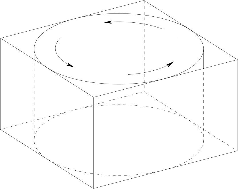
Inside the computational box, the plasma is rotating in the horizontal plane about an axis passing through the centre. The rotation speed $\Omega$ is independent of distance from the axis $\varpi$ and a function of just height $z$. The bottom face of the box lies in the plane $z=0$. The computational box has a height $L$ and width $2L$.

We use a system of Cartesian coordinates. At first glance one might instead consider using cylindrical coordinates, as these appear to be more suited to the task. This is indeed the case if one is wanting to handle the problem analytically. However, cylindrical coordinates not only make numerical modelling more time-consuming per grid box, but also introduce special points (the axis). This coordinate singularity is a known problem in all grid-based codes in cylindrical and spherical coordinates. Since the phenomenon we wish to investigate lies on the z-axis, it is better to use Cartesians so that we can be sure that our results are not merely an artefact of the code. The disadvantage is that some space in the corners of the computational box is wasted. When the output of the code is analysed, a conversion into cylindrical coordinates is first performed. The computational setup is illustrated in Fig. 1.

Figure 1: The computational box. The cylinder represents the volume where the gas is being acted on by the rotational force in Eq. (13).

2.1 Implementation of the differential rotation

We want the rotation rate of the gas to have a time-average dependence on height of the form $\Omega=\Omega_{0}+z{\rm d}\Omega/{\rm d}z$. To achieve this we apply a force $\mathbf{F}$ per unit mass of the form:

$$\mathbf{F}(\varpi,z)=(\mathbf{v}_{0}-\mathbf{v})/\tau_{\mathrm{f}}\qquad{\rm where}\qquad\mathbf{v}_{0}=\frac{{\rm d}\Omega}{{\rm d}z}z\varpi\mathbf{e}_{\phi}$$ (13)

where $\mathbf{v}$ is the velocity field, $\tau_{\mathrm{f}}$ is a time-scale, which can be chosen, and $\mathbf{e}_{\phi}$ is the azimuthal unit vector. No force was applied in the vertical direction. The gas at $z=0$ is therefore not rotating. We could in principle add a constant $\Omega_{0}$ to the rotation speed, but this would result in the gas moving more quickly, and the time step of the code would go down. It is better to include $\Omega_{0}$ indirectly: we transform to the rotating frame and add the Coriolis force $2\mathbf{v\times\Omega}_{0}$ to the momentum equation. The centrifugal force can be ignored since its only effect would be a change in the equilibrium state.

This force $\mathbf{F}$ is applied to the gas out to a radius $L$, i.e. to the sides of the computational box. This means that the corners escape this force. This was found to be the best way to reduce the effect of the geometry of the box on the physical phenomenon of interest – the gas in the corners is roughly stationary and its effect on the rotating gas in the middle is minimal.

In a star, differential rotation is driven by two mechanisms: magnetic braking, which acts on the surface of the star, and evolution, when radial shells are contracting and expanding. The former would be difficult to model, as exerting a force at the boundaries could be expected to cause problems at those boundaries. Exerting a torque by means of a distributed force, as is done here, is a good way to model differential rotation caused by evolution.

2.2 Boundary conditions

In all three directions, we employ mirror-like boundary conditions. This means that unknown quantities just outside the boundaries are copied from the same quantities just inside the same boundary. This is somewhat more difficult to implement than the periodic conditions used in Braithwaite (2005), but is necessary for the following reason. The gas in this case is rotating in a horizontal plane; with periodic boundary conditions the gas at the boundary would be moving in the opposite direction to the gas immediately adjacent on the other side of the boundary. This would cause turbulence – we are only interested in one kind of instability and introducing another would surely confuse the issue. In fact, periodic boundary conditions were tried at first, and it was found that a dynamo process was produced even in the case of uniform rotation (${\rm d}\Omega/{\rm d}z=0$), as a result of the hydrodynamic turbulence created at the boundaries. This argument does not of course hold at the boundaries in the vertical direction, but there is a good reason for having the same conditions there. Sound and internal gravity waves can propagate upwards, their amplitude growing as they do so. With periodic conditions at the vertical boundaries, a wave can go through the top of the computational box and come back at the bottom, to continue its upwards travel. Its amplitude rises exponentially on a timescale roughly equal to $N^{-1}$ and will eventually get out of control. In Braithwaite (2005) we prevented this by having gravity point in opposite directions in the top and bottom halves of the volume modelled, the drawback being the computational expense of having to model the same thing twice. The method used in this study is, as far the the end result in concerned, the same as that previous method, but computational cost has been exchanged for programming complexity.

2.3 Initial conditions

We begin with uniform temperature; pressure decreases exponentially with increasing $z$, in hydrostatic equilibrium. The initial velocity field we create by running the code with no magnetic field until a steady state has been reached. The initial magnetic field should in principle be unimportant, except that it must have a vertical component and must be weak. We choose therefore the simplest field imaginable: a uniform vertical field $\mathbf{B}=B_{0}\mathbf{e}_{z}$, where $\mathbf{e}_{z}$ is the vertical unit vector. The field energy must be weak compared to both the thermal energy and the kinetic energy, or in other words, the Alfvén speed must be much less than both the sound speed and the rotation speed. $B_{0}$ is chosen so that the ratio of thermal to magnetic energy densities $\beta=10^{5}$, or so that the ratio of sound to Alfvén speeds is $240$. The ratio of rotation speed to Alfvén speed depends of course on the values we choose for $\Omega_{0}$ and ${\rm d}\Omega/{\rm d}z$. We want the gas to be rotating as fast as possible (to maximize the chances of creating a dynamo) but still comfortably below the sound speed. With a magnetic field this weak, there is still plenty of space to fit the rotation time scale between the sound and Alfvén time scales.

2.4 Free parameters

The goal is to produce a self-sustaining magnetic field, but there are few clues as to precisely what conditions may be necessary. We have a fair number of parameters to play with.

The values of $\Omega_{0}$ and ${\rm d}\Omega/{\rm d}z$ will have an effect. It is expected that a value of $\Omega_{0}$ above $\omega_{\rm A}$ will slow the growth rate of the Tayler instability. This would then increase the saturation field strength. Whether this makes a dynamo any more or less likely to appear in our model is not clear. What is certain, however, is that a large value of ${\rm d}\Omega/{\rm d}z$ will be conducive to the appearance of a self-sustaining field. We set this therefore in all runs to a high value but such that the flow speed is still comfortably below the sound speed. We set ${\rm d}\Omega/{\rm d}z=c_{\rm s}/5L^{2}$, so that the gas is moving at a maximum of one fifth of the sound speed.

Another choice to be made is the relaxation time-scale $\tau_{\rm f}$ of the driving force. Setting it too low would inhibit the instability, as it would hold the plasma to too stiff a velocity field. Too high a value, on the other hand, may mean that the driving force is insufficient to make the plasma rotate in the required manner. Various values are used in the results reported below.

The code contains an artificial diffusion scheme designed to maintain stability. It includes terms for all three diffusivities (kinetic, thermal and magnetic). The adjustable coefficients in this scheme were set to the experimentally determined minimum value needed for numerical stability. In the simulations presented in Braithwaite (2005), it was possible to turn off this scheme completely, since we were dealing with a body of plasma which was stationary at $t=0$ and whose movement we only wished to follow while the velocities were small. This is unfortunately not the case here, as the plasma is necessarily moving fairly quickly.

In an ideal simulation, all unstable wavenumbers would be modelled between the two limits in Eq. (4). The wavenumbers accessible numerically are given by the vertical size of the computational box and the spatial resolution (the Nyquist spatial frequency):

$$\frac{\pi}{{\rm d}z}>n>\frac{2\pi}{L}$$ (14)

To see an instability at all, we need this numerical range to overlap with 14.

3 The numerical code

We use a three-dimensional MHD code developed by Nordlund & Galsgaard (1995), with extensive modifications, chiefly the mirror-like boundary conditions described in Sect. 2.2. The code uses a staggered mesh, so that variables are defined at different points in the grid-box. For example, $\rho$ is defined in the centre of each box, but $u_{x}$ in the centre of the face perpendicular to the x-axis, so that the value of $x$ is lower by $\frac{1}{2}{\rm d}x$. Interpolations and spatial derivatives are calculated to fifth and sixth order respectively. The third order predictor-corrector time-stepping procedure of Hyman (1979) is used.

The high order of the discretization is a bit more expensive per grid point and time step, but the code can be run with fewer grid points than lower order schemes, for the same accuracy. Because of the steep dependence of computing cost on grid spacing (4th power for explicit 3D) this results in greater computing economy.

For stability, high-order diffusive terms are employed. Explicit use is made of highly localised diffusivities, while retaining the original form of the partial differential equations.

4 Results

We present results for a number of different setups. First, we look at the unstratified case, both with and without rotation ($\Omega_{0}=0$ and $\Omega_{0}\neq 0$). Then, the stratified case, again both with and without rotation.

We ran the code with $64$ grid points in the horizontal directions and $32$ in the vertical. This is a trade-off between the resolution needed to obtain dynamo action and the large number of time steps needed. The time step is set by the sound crossing time, but the (Alfvénic) time-scales of interest to us are necessarily much longer. As explained, the high order of the spatial discretization of the code guarantees a high effective resolution even at this limited number of grid points, and self-sustained magnetic fields were readily obtained at this resolution in all cases studied.

4.1 An unstratified case

In the absence of gravity, there is no maximum to the vertical length scales that are unstable (see Eq. (4)). Since it is the maximum unstable wavelength which determines how quickly the field is wound up, the dynamo never becomes saturated; the field simply continues to grow until it is strong enough to kill the differential rotation.

However, the fact that we are conducting this simulation inside a box of finite dimensions changes things somewhat, by imposing an artificial maximum wavelength. This enables the field to find a saturation level, and the instability operates at the largest length scale that fits into the numerical box.

With the unstratified setup, the production of a statistically steady, self-sustained magnetic field was observed. To understand the properties of the field produced, it is useful to see the evolution of the mean magnetic energy density, split up into its poloidal and toroidal components. To this end, $B_{\phi}^{2}/8\pi$ and $B_{p}^{2}/8\pi=(B_{z}^{2}+B_{\varpi}^{2})/8\pi$ are plotted in Fig. 2. The time on the horizontal axis of this graph is expressed in units of the sound-crossing time $\tau_{\rm s}=L/c_{\rm s}$. The field, initially poloidal, becomes mainly toroidal as it is wound up by the differential rotation. This happens very quickly, over the time-scale $\tau_{\rm dr}$. Both components then grow, more slowly, until the saturation level is reached, when the field is being destroyed by the instability at the same rate at which it is being amplified by the differential rotation.

Fig. 3 shows contour plots of the vertical component of the magnetic field $B_{z}$ and of the azimuthal component $B_{\phi}$, averaged in the azimuthal direction, as a function of $\varpi$ and $z$. The nine panels are taken at nine different times: $t=513$, $664$, $694$, $724$, $754$, $785$, $815$, $845$ and $875\tau_{\rm s}$ (in units of the sound crossing time across the box). At the time of the first frame, the azimuthal mean of $B_{z}$ is positive everywhere, as it is at the beginning of the run. $B_{\phi}$ has been produced from the winding-up of this positive $B_{z}$ by differential rotation of positive ${\rm d}\Omega/{\rm d}z$, so is also positive almost everywhere. Then the instability produces a new vertical component which points predominantly downwards: $B_{z}$ switches from positive to negative. The azimuthal component does likewise.

Figure 2: Amplitude of the self-sustained magnetic field in an unstratified case with maximum shear velocity 1/5 of the sound speed. Averages of $B_{\phi}^{2}/8\pi$ (solid line) and $B_{p}^{2}/8\pi$ (dotted line), in units of the thermal energy density. The field is predominantly toroidal. Time is in units of $\tau_{\rm s}$, the sound crossing time of the box.

Figure 3: Azimuthal average of $B_{z}$ (positive values shaded light, negative dark), as a function of $\varpi$ (horizontal axis) and $z$ (vertical axis). Contours show $B_{\phi}$ (black lines, with ticks pointing towards negative values). The thick lines show where $B_{z}$ and $B_{\phi}$ are equal to zero. The nine panels are taken at nine different times: $t=513$, $664$, $694$, $724$, $754$, $785$, $815$, $845$ and $875\tau_{\rm s}$, arranged top-left, top-middle, top-right, middle-left, etc. The predominant sign of polarities of both $B_{z}$ and $B_{\phi}$ changes over this period. Unstratified case ($N=0$).

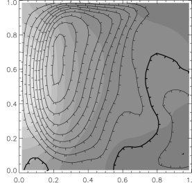
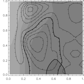
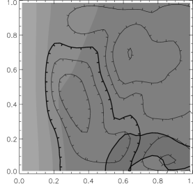
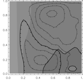
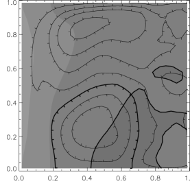
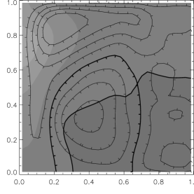
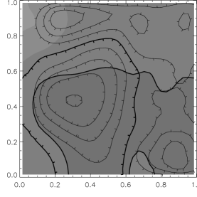
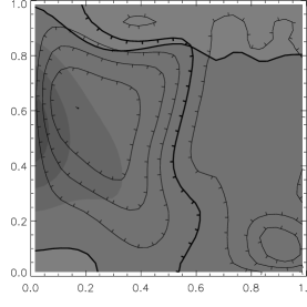
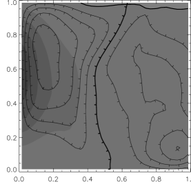
Looking at Fig. 2, it can be seen that the mean field strength is lower than usual during this reversal period. This reversal in the prevailing direction of the field happens three times during this run (also at $t=2200$ and $3000\tau_{\rm s}$), and there is no reason not to presume that it should continue to happen were the run continued.

A change of the field direction throughout the entire cylindrical volume is not surprising when one takes into account the fact that only the longest wavelengths are unstable. Most of the unstable range of wavelengths lies outside of the range which can be seen in this simulation – we cannot see unstable wavelengths longer than the size of the computational box. In reality, we would see instability over a range of length scales; in this unstratified case, up to infinity.

4.1.1 Torques

The torques produced by the dynamo process vary through the box. As an average measure of the magnetic torque, we integrate the azimuthal component of the Lorentz shear stress, multiplied by the lever arm $\varpi$, over a horizontal plane. We want to check that the torque acting on the plasma really is magnetic in origin, and not kinetic, since the velocity field also produces a shear stress. We calculate the two respective torques in the following way:

$$T_{\rm m}(z,t) = \int_{\phi=0}^{2\pi}\varpi\,{\rm d}\phi\int_{\varpi=0}^{L}{\rm d}\varpi\,\varpi\frac{B_{\phi}B_{z}}{4\pi},$$ (15)

$$T_{\rm v}(z,t) = \int_{\phi=0}^{2\pi}\varpi\,{\rm d}\phi\int_{\varpi=0}^{L}{\rm d}\varpi\,\varpi\rho v_{\phi}v_{z}.$$ (16)

The averages over $z$ of these two torques are plotted in Fig. 4. This confirms that the torque is chiefly magnetic. The torque from the velocity field is almost ten time smaller, sometimes even negative, i.e. it has the effect of increasing the differential rotation.

The torques $T_{\rm m}$ and $T_{\rm v}$ are plotted in units of $(2/3)\pi PL^{3}$; this is the torque which would exist if the shear stress were equal to the gas pressure $P$. In accretion disk parlance, this corresponds to a viscosity paramater $\alpha=1$. In fact, it is of some interest to compare the shear stress in this model to that found in an accretion disc, since they are caused by similar processes. That the stress in an accretion disc is of the order of the gas pressure should not be surprising, since the kinetic energy of the orbital motion, which drives the dynamo, is of the same order as the thermal energy. In a differentially rotating star, however, the energy available to power the dynamo (the difference in kinetic energy compared with a uniformly rotating star with the same angular momentum), is much less than the thermal energy. We should therefore also expect the magnetic energy to be much less than the thermal energy, as it cannot be greater than the energy of differential rotation.

Figure 4: Mean torque from the magnetic field $T_{\rm m}$ (solid line) and the velocity field $T_{\rm v}$ (dotted line), in units of $(2/3)\pi PL^{3}$. Non-stratified ($N=0$), non-rotating ($\Omega_{0}=0$) case.

We have seen that the torque exerted by the magnetic field is much less than the torque which would exist if the shear stress were equal to the gas pressure, as we expected. A more interesting quantity to compare it to, in this context, is the torque which would exist if the shear stress were equal to the magnetic pressure $B^{2}/8\pi$. To do this, we calculate a dimensionless efficiency coefficient $\epsilon$, defined such that:

$$T_{\rm m}(z,t)=\epsilon(z,t)\int_{\phi=0}^{2\pi}\varpi\,{\rm d}\phi\int_{\varpi=0}^{L}{\rm d}\varpi\,\varpi\frac{B^{2}}{8\pi}.$$ (17)

This efficiency $\epsilon$, or rather, the average of it over all $z$, is plotted is Fig. 5. After the initial winding-up phase, its value tends to stay at around $0.08$, except for the field-reversal phases when the field is weaker.

Figure 5: Efficiency coefficient $\epsilon$, as defined in Eq. (17) for the run shown in Fig. 4

If the vertical and azimuthal component of the field were everywhere equal, and if the component in the $\varpi$ direction were zero, we would have $\epsilon=1$. As in the case of MRI turbulence in accretion disks, however, the field is mainly azimuthal. Comparing Eqs. (15) and (17), and assuming that the ratio $B_{\phi}/B_{z}$ is the same everywhere and that $B_{\varpi}=0$:

$$\epsilon\approx\frac{B_{\phi}B_{z}/4\pi}{B^{2}/8\pi}\approx\frac{2(B_{\phi}/B_{z})}{1+(B_{\phi}/B_{z})^{2}}.$$ (18)

Looking at Fig. 2, we can estimate that $B_{\phi}/B_{z}\approx 1.8$, and the above equation gives us $\epsilon\approx 0.8$. The main reason for the low torque efficiency may then be that the ratio $B_{\phi}/B_{z}$ is not constant, rather, it is low at small $\varpi$ and high at large $\varpi$. This is confirmed by looking at the last frame of Fig. 3, for instance: $B_{z}$ is strongest very close to the axis, as the Tayler instability is strongest there, and $B_{\phi}$ is strongest somewhat further from the axis, because the winding-up effect is stronger at larger $\varpi$.

4.1.2 Parameter dependence

For the run discussed above the net rotation $\Omega_{0}=0$, (the rotation rate at $z=0$, the middle of the box), and the damping time of the applied force $\tau_{\rm f}$ was set equal to the sound crossing time $\tau_{\rm s}$. For values of $\tau_{\rm f}$ much different from this, a self-sustaining field was not produced. If too low a value is used, the velocity field is too ‘stiff’ and the instability is unable to take hold, although the field does reach the required strength. If $\tau_{\mathrm{f}}$ is too high, on the other hand, the differential rotation is slowed down by the Lorentz forces from the magnetic field before the necessary field strength for instability has been reached.

The code was run with a range of values of $\tau_{\mathrm{f}}/\tau_{\rm s}$: $0.1$, $1.0$, $10$ and $100$. Fig. 6. shows the evolution of the mean magnetic energy density $B^{2}/8\pi$. It can be seen that a self-sustaining field was observed only around $\tau_{\mathrm{f}}/\tau_{\rm s}=1$. It was also found that the dynamo is not produced if a lower spatial resolution is used. It therefore seems that where the dynamo was produced, the conditions were only just sufficient. So it should not be surprising that it also only works in a narrow range of the parameter $\tau_{\mathrm{f}}$. A higher spatial resolution will be needed to obtain dynamo action in a less restricted range of parameter values.

Figure 6: Mean magnetic energy density against time, for runs with $N=0$ and $\tau_{\mathrm{f}}/\tau_{\rm s}=$ $0.1$ (solid line), $1.0$ (dotted), $10$ (dashed) and $100$ (dot-dashed). Energy density is in units of the thermal energy density, time in sound crossing times $\tau_{\rm s}$. Only in a narrow range of $\tau_{\mathrm{f}}/\tau_{\rm s}$ is a statistically steady magnetic field maintained.

4.1.3 Rotation

In the above we have shown a working dynamo in simulations with differential rotation, but with no rotation overall. This is of course unlikely to be the situation inside a real star, so we shall now model a plasma with a net rotation by adding a Coriolis force to the momentum equation. We find that rotation above a certain speed is able to stop the dynamo from working, presumably because with the given resolution it is only just possible to see the instability working, and small changes can push the dynamo action just outside the effective range. We shall see in the next section that in the stratified case the dynamo is more vigorous; active in a less restricted range of parameters.

We run the code as above, but with values of $\Omega_{0}$ which will put us into the $\Omega\gg\omega_{\mathrm{A}}$ regime: $\Omega_{0}/\tau_{\rm s}^{-1}=0.1$, $0.3$ and $1.0$. Fig. 7 shows the magnetic energy density as a function of time, for these runs, as well as for the $\Omega_{0}=0$ run. It can be seen that when the rotation speed is above some certain threshold, the field, although still wound up at first, decays again without reaching a steady state. This behavior is not fully understood. It is expected that rotation will slow the growth of the instability, and will therefore increase the minimum unstable wavelength (Eq. (4)), which depends on diffusivity. This could mean that the field never becomes unstable.

Figure 7: Mean magnetic energy density against time, for $N=0$ runs with forcing parameter $\Omega_{0}/\tau_{\rm s}^{-1}=$ $0$ (solid line), $0.1$ (dotted), $0.3$ (dashed) and $1.0$ (dot-dashed). Energy density in units of the mean thermal energy density. Sustained magnetic fields are obtained only at the lower rotation rates.

4.2 The stratified case

In the stratified case, the additional parameter is the buoyancy frequency $N$. The main result will turn out to be that a self-sustaining magnetic field is much easier to create in the stratified case. Whereas in the unstratified case, a self-sustained field was only produced within a narrow range of parameters, with stratification the range of parameters is now much wider. Rotation does not destroy the dynamo, even for rotation frequency $\Omega$ as large as the buoyancy frequency.

There are one or two other differences. The field builds up to saturation much more slowly – in the unstratified case, saturation was reached over one or two Alfvén crossing times (Alfvén crossing times at the initial field strength). In the stratified case, it takes at least five times longer. Also, the field energy is much steadier; the fluctuations do not seem to be as large.

Figure 8: The means of $B_{\phi}^{2}/8\pi$ (solid line) and $B_{p}^{2}/8\pi$ (dotted line), in units of the thermal energy density, for a stratified case $N=\tau_{\rm s}^{-1}$. The field is even more predominantly toroidal than in the unstratified case (compare Fig. 2).

Fig. 8 shows the toroidal and poloidal components of the magnetic energy, for a run with $N=\tau_{\rm s}^{-1}$ and $\tau_{\rm f}=10\tau_{\rm s}$. The energy in the toroidal component is around $30$ times larger than that in the poloidal component, a larger difference than in the absence of stratification (cf. Fig. 2).

As in Sect. 4.1.1, we calculate an efficiency coefficient $\epsilon$ (see Eq. (17)). This is plotted in Fig. 9 for this stratified run. The value settles a little lower than in the unstratified case, at around $0.05$. In this case, however, the ratio $B_{\phi}/B_{z}$ is much greater (comparing Figs. 2 and 8), so we expect a lower efficiency $\epsilon$. The reason that the same value of $\epsilon$ is measured despite a higher average of the ratio $B_{\phi}/B_{z}$ must have something to do with the respective distributions as a function of $\varpi$ of the vertical and azimuthal components of the field.

We can try using other values of the driving-force time-scale $\tau_{\rm f}$, to see how robust the dynamo is. For these runs, we used a somewhat stronger initial magnetic field, with $\beta=10^{3}$, as opposed to $\beta=10^{5}$ used in the previous runs. This helps to speed up the initial evolution a little, but has no effect on the final steady state.

We use values of $\tau_{\rm f}/\tau_{\rm s}$ of $1$, $10$ and $100$. In this last case, the time-scale $\tau_{\rm f}$ is much greater than other relevant time-scales, which will also be the case in a real star. The magnetic energy in these runs is plotted in Fig. 10. A self-sustaining field appears in all three cases, although the saturation field strength does depend to some extent on the value of $\tau_{\rm f}$. This in fact does reflect reality – the faster the differential rotation is being driven, the stronger we expect the excited field to be.

Figure 9: Efficiency coefficient $\epsilon$, as defined in Eq. (17). Stratified ($N=\tau_{\rm s}^{-1}$), non-rotating case.

Figure 10: Mean magnetic energy density against time, for the stratified case $N=\tau_{\rm s}^{-1}$. $\tau_{\rm f}/\tau_{\rm s}=$ $1$ (solid line), $10$ (dotted) and $100$ (dashed). A self-exciting field is produced in all three cases.

Figure 11: Mean magnetic energy density against time, for a rotating, stratified case. $\tau_{\rm f}/\tau_{\rm s}=$ $1$ (solid line), $10$ (dotted) and $100$ (dashed). A self-exciting field is produced in all three cases, and a oscillatory behavior is seen in one case.

We have now looked at three cases: non-rotating unstratified; rotating unstratified; and non-rotating stratified. The fourth combination – rotating stratified ($\Omega\gg\omega_{\rm A}$ and $N\gg\omega_{\rm A}$) – will exist in almost the entire non-convective zone of almost all stars, and is therefore the most interesting to us. To be sure that we are in this regime, we shall set both $N$ and $\Omega_{0}$ to the reciprocal of the sound-crossing time, i.e. to $\tau_{\rm s}^{-1}$.

It is found that the self-sustaining field is still produced, unlike when rotation was added to the unstratified case. The field produced is of comparable strength to that produced when rotation is absent, but oscillates in a seemingly regular fashion. The mean values of $B_{\phi}$ and $B_{z}$ go from positive to negative, and back again. We saw something like this in Sect. 4.1, but there, the reversal of the field was a more chaotic process with, one presumes, no regular period. Fig. 11 is the rotating equivalent of Fig. 10. Except at the highest value of $\tau_{\rm f}$, the field energy can be seen to jump up and down in a regular way.

5 Discussion and Conclusions

We have demonstrated by direct numerical simulation a dynamo process as envisaged by analytical arguments in Spruit (2002). It feeds off differential rotation only, and not from any imposed small-scale velocity field. The toroidal (azimuthal) component of the field is produced from the winding-up of the existing poloidal (meridional) component. This toroidal field is unstable, and produces, as a result of its decay, a new poloidal component, which can then be wound up itself – in this way, the ‘dynamo loop’ is closed. A weak seed field is amplified in this way until a certain saturation level is reached, at which the field is being wound up by differential rotation at the same rate as it is decaying through its inherent magnetohydrodynamic instability.

This dynamo is therefore different from the traditional convection-powered dynamo models for stars with convective envelopes, in which the dynamo loop is closed by poloidal components induced by an additional, non-magnetic process. The dynamo found here is, in this sense, similar to the MRI turbulence in accretion disk (Hawley et al. (1996)) which is powered by the gradient in orbital rotation in the disk.

A dominant factor in the case of differential rotation in a star is the effect of the stable stratification. It strongly restricts the types of instability that can occur in the azimuthal field produced by winding up in the differential rotation. In Spruit (1999) we have shown that the first instability to set in as the magnetic field strength increases by this process is Tayler-instability (a pinch-type instability) rather than magnetic buoyancy instabilities.

In the simulations presented here we have considered separately the effects of rapid net rotation and a stabilizing stratification. Perhaps somewhat surprisingly, dynamo action was found to set in more readily (at lower spatial resolution) in the stratified cases than in the unstratified case. This is the opposite of what would be expected if buoyancy instabilities were the dominant mechanism closing the dynamo loop. This confirms the conclusion in Spruit (2002) that differential rotation in a stable stratification leads to a self-sustained magnetic field in which Tayler instability of the azimuthal field is the dominant process closing the dynamo cycle.

The results presented were obtained only at a resolution close to the minimum required to obtain dynamo action. As a result, the field configurations obtained show only minimal structure in the vertical direction. Effectively, they cover only vertical length comparable with the characteristic vertical length scale of the process (which is governed by the strength of the stratification, cf. Spruit 2002).

For further progress, simulations at higher resolution will allow more detailed comparison with the analytical estimates. An important step forward, however, would be the development of code more suited to the nearly-incompressible, highly stratified conditions relevant for stellar interiors. With the existing codes, the time step limitations due to sound speed and the buoyancy frequency limit the degree of realism that can be achieved.

References

- Acheson (1978) Acheson, D.J., 1978, Phil. Trans. Roy. Soc. Lond., A289, 459.
- (2) Braithwaite, J., 2005, A&A, submitted
- Charbonneau et al. (1999) Charbonneau, P., Christensen-Dalsgaard, J., Henning, R. et al., 1999, ApJ, 527, 445.
- Hawley et al. (1996) Hawley, J.F., Gammie, C.F. and Balbus, S.A., 1996, ApJ, 464, 690.
- Heger et al. (2003) Heger, A., Woosley, S.E., Langer and N., Spruit, H.C., 2003, Proc. IAU Symp. No. 215.
- Hyman (1979) Hyman, J., 1979, in R. Vichnevetsky, R.S. Stepleman (eds.), Adv. in Comp. Meth. for PDEs - III, 313.
- Maeder & Meynet (2003) Maeder, A. and Meynet, G., 2003, A&A, 411, 543.
- Mestel (1953) Mestel, L., 1953, MNRAS, 113, 716.
-
Nordlund & Galsgaard (1995)
Nordlund, Å. and
Galsgaard, K., 1995,
http://www.astro.ku.dk/aake/papers/95.ps.gz - Parker (1979) Parker, E.N., 1979, “Cosmological magnetic fields: their origin and their activity”, Oxford, Clarendon Press.
- Schou et al. (1998) Schou, J., Antia, H.M., Basu, S. et al., 1998, ApJ, 505, 390.
- Spruit (1999) Spruit, H. C., 1999, A&A, 349, 189.
- Spruit (2002) Spruit, H. C., 2002, A&A, 381, 923.
- Tayler (1973) Tayler, R.J., 1973, MNRAS, 161, 365.