Quantitative Spectroscopy of BA-type Supergiants

Luminous BA-type supergiants have enormous potential for modern astrophysics. They allow topics ranging from non-LTE physics and the evolution of massive stars to the chemical evolution of galaxies and cosmology to be addressed. A hybrid non-LTE technique for the quantitative spectroscopy of these stars is discussed. Thorough tests and first applications of the spectrum synthesis method are presented for the bright Galactic objects $\eta$ Leo (A0 Ib), HD 111613 (A2 Iabe), HD 92207 (A0 Iae) and $\beta$ Ori (B8 Iae), based on high-resolution and high-S/N Echelle spectra. Stellar parameters are derived from spectroscopic indicators, consistently from multiple non-LTE ionization equilibria and Stark-broadened hydrogen line profiles, and they are verified by spectrophotometry. The internal accuracy of the method allows the 1$\sigma$-uncertainties to be reduced to $\lesssim$1–2% in $T_{\rm eff}$ and to 0.05–0.10 dex in $\log g$. Elemental abundances are determined for over 20 chemical species, with many of the astrophysically most interesting in non-LTE (H, He, C, N, O, Mg, S, Ti, Fe). The non-LTE computations reduce random errors and remove systematic trends in the analysis. Inappropriate LTE analyses tend to systematically underestimate iron group abundances and overestimate the light and $\alpha$-process element abundances by up to factors of two to three on the mean. This is because of the different responses of these species to radiative and collisional processes in the microscopic picture, which is explained by fundamental differences of their detailed atomic structure, and not taken into account in LTE. Contrary to common assumptions, significant non-LTE abundance corrections of $\sim$0.3 dex can be found even for the weakest lines ($W_{\lambda}$ $\lesssim$ 10 mÅ). Non-LTE abundance uncertainties amount to typically 0.05–0.10 dex (random) and $\sim$0.10 dex (systematic 1$\sigma$-errors). Near-solar abundances are derived for the heavier elements in the sample stars, and patterns indicative of mixing with nuclear-processed matter for the light elements. These imply a blue-loop scenario for $\eta$ Leo because of first dredge-up abundance ratios, while the other three objects appear to have evolved directly from the main sequence. In the most ambitious computations several ten-thousand spectral lines are accounted for in the spectrum synthesis, permitting the accurate reproduction of the entire observed spectra from the visual to near-IR. This prerequisite for the quantitative interpretation of intermediate-resolution spectra opens up BA-type supergiants as versatile tools for extragalactic stellar astronomy beyond the Local Group. The technique presented here is also well suited to improve quantitative analyses of less extreme stars of similar spectral types.

1 Introduction

Massive supergiants of late B and early A-type (BA-type supergiants, BA-SGs) are among the visually brightest normal stars in spiral and irregular galaxies. At absolute visual magnitudes up to $M_{V}$ $\simeq$ $-$9.5 they can rival with globular clusters and even dwarf spheroidal galaxies in integrated light. This makes them primary candidates for quantitative spectroscopy at large distances and makes them the centre of interest in the era of extragalactic stellar astronomy. The present generation of 8–10m telescopes and efficient multi-object spectrographs can potentially observe individual stars in systems out to distances of the Virgo and Fornax cluster of galaxies (Kudritzki Kudritzki98, Kudritzki00). The first steps far beyond the Local Group have already been taken (Bresolin et al. Bresolinetal01, Bresolinetal02; Przybilla Przybilla02).

BA-type supergiants pose a considerable challenge for quantitative spectroscopy because of their complex atmospheric physics. The large energy and momentum density of the radiation field, in combination with an extended and tenuous atmosphere, gives rise to departures from local thermodynamic equilibrium (non-LTE), and to stellar winds. Naturally, this makes BA-SGs interesting in terms of stellar atmosphere modelling and non-LTE physics, but there is more to gain from their study. They can be used as tracers for elemental abundances, as their line spectra exhibit a wide variety of chemical species, ranging from the light elements to $\alpha$-process, iron group and s-process elements. These include, but also extend the species traced by H ii-regions and thus they can be used to investigate abundance patterns and gradients in other galaxies to a far greater extent than from the study of gaseous nebulae alone. In fact, stellar indicators turn out to be highly useful for independently constraining (Urbaneja et al. Urbanejaetal05) the recently identified systematic error budget of strong-line analyses of extragalactic metal-rich H ii regions (Kennicutt et al. Kennicuttetal03; Garnett et al. Garnettetal04; Bresolin et al. Bresolinetal04), and its impact on models of galactochemical evolution. BA-type supergiants in other galaxies allow the metallicity-dependence of stellar winds and stellar evolution to be studied. In particular, fundamental stellar parameters and light element abundances (He, CNO) help to test the most recent generation of evolution models of rotating stars with mass loss (Heger & Langer HeLa00; Meynet & Maeder MeMa00; MeMa03; MeMa05; Maeder & Meynet MaMe01) and in addition magnetic fields (Heger et al. Hegeretal05; Maeder & Meynet MaMe05). These make predictions about the mixing of the stellar surface layers with nuclear processed matter which can be verified observationally. Moreover, BA-SGs can act as primary indicators for the cosmological distance scale by application of the wind momentum–luminosity relationship (WLR, Puls et al. Pulsetal96; Kudritzki et al. Kudritzkietal99) and by the flux-weighted gravity–luminosity relationship (FGLR, Kudritzki et al. Kudritzkietal03; Kudritzki & Przybilla KuPr03). In addition to the stellar metallicity, interstellar reddening can also be accurately determined, so that BA-SGs provide significant advantages compared to classical distance indicators such as Cepheids and RR Lyrae.

Despite this immense potential, quantitative analyses of BA-SGs are scarce. Only a few single objects were studied in an early phase; several bright Galactic supergiants, preferentially among these $\alpha$ Cyg (A2 Iae) and $\eta$ Leo (Groth Groth61; Przybylski Przybylski69; Wolf Wolf71; Aydin Aydin72) and the visually brightest stars in the Magellanic Clouds (Przybylski Przybylski68, Przybylski71, Przybylski72; Wolf Wolf72, Wolf73). Near-solar abundances were found in almost all cases. Surveys for the most luminous stars in the Local Group galaxies followed (Humphreys Humphreys80, and references therein), but were not accompanied by detailed quantitative analyses. These first quantitative studies were outstanding for their time, but from the present point of view they were also restricted in accuracy by oversimplified analysis techniques/model atmospheres, inaccurate atomic data and the lower quality of the observational material (photographic plates). Non-LTE effects were completely ignored at that time, as appropriate models were just being developed (e.g. Mihalas Mihalas78, and references therein; Kudritzki Kudritzki73).

BA-type supergiants have become an active field of research again, following the progress made in model atmosphere techniques and detector technology (CCDs), and in particular the advent of 8–10m-class telescopes. In a pioneering study by Venn (Venn95a, Venn95b) over twenty (less-luminous) Galactic A-type supergiants were systematically analysed for chemical abundances, using modern LTE model atmosphere techniques, and non-LTE refinements in a few cases. These indicated near-solar abundances for the heavier elements and partial mixing with CN-cycled gas. A conflict with stellar evolution predictions was noted, as the observed high N/C ratios were realised through carbon depletion and not via the predicted nitrogen enrichment. Later, this conflict was largely resolved by Venn & Przybilla (VePr03). However, an analysis of helium was not conducted, and more luminous supergiants, which are of special interest for extragalactic studies, were missing in the sample. Similar applications followed on objects in other spiral and dwarf irregular galaxies (dIrrs) of the Local Group (McCarthy et al. McCarthyetal95; Venn Venn99; Venn et al. Vennetal00, Vennetal01, Vennetal03) and the nearby Antlia-Sextans Group dIrr galaxy Sextans A (Kaufer et al. Kauferetal04). The primary aim was to obtain first measurments of heavy element abundances in these galaxies. Good agreement between stellar oxygen abundances and literature values for nebular abundances was found, with the exception of the dIrr WLM (Venn et al. Vennetal03). The number of objects analysed is small, thus prohibiting the derivation of statistically significant further conclusions. Moreover, abundances of the mixing indicators He, C and N were not determined in almost all cases.

Parallel to this, a sample of Galactic BA-SGs were studied by Takeda & Takada-Hidai (TaTa00, and references therein) for non-LTE effects on the light element abundance analyses which confirm the effects of mixing in the course of stellar evolution. However, a conflict with the predictions of stellar evolution models was found, because C depletion was apparently accompanied by He depletion. The authors regarded this trend not being real, but indicated potential problems with the He i line-formation. On the other hand, stellar parameters were not independently determined in these studies, but estimated, which can result in severe systematic global errors as will be shown later. Verdugo et al. (Verdugoetal99b) concentrated on deriving basic stellar parameters for over 30 Galactic A-type supergiants, assuming the validity of LTE. Independently, the Galactic high-luminosity benchmark $\alpha$ Cyg was investigated for elemental abundances by Takeda et al. (Takedaetal96), solving the restricted non-LTE problem, and by Albayrak (Albayrak00), using a pure LTE approach. Fundamental parameters of $\alpha$ Cyg were determined by Takeda (Takeda94) and by Aufdenberg et al. (Aufdenbergetal02). At lower luminosity, $\eta$ Leo was the subject of a couple of such studies (Lambert et al. Lambertetal88; Lobel et al. Lobeletal92). The results from these studies mutually agree only if rather generous error margins are allowed for, implying considerable systematic uncertainties in the analysis methods. Among the late B-type supergiants the investigations focused on $\beta$ Ori (Takeda Takeda94; Israelian et al. Israelianetal97). A larger sample of Galactic B-type supergiants, among those a number of late B-types, was studied by McErlean et al. (McErleanetal99) for basic stellar parameters and estimating elemental abundances, on the basis of unblanketed non-LTE model atmospheres and non-LTE line formation. The chemical analysis recovers values being consistent with present-day abundances from unevolved Galactic B-stars, except for the light elements, which again indicate mixing of the surface layers with material from the stellar core.

Figure 1: Spectra of the sample stars around H$\gamma$ and H$\alpha$. The major spectral features are identified, short vertical marks indicate Fe ii lines. Luminosity increases from bottom to top. Likewise, H$\alpha$ develops from a pure absorption line into a P-Cygni-profile because of the strengthening stellar wind. Note the marked incoherent electron scattering wings of H$\alpha$ in the most luminous object.

The basic stellar parameters and abundances from modern studies of individual objects can still be discrepant by up to $\sim$20% in $T_{\rm eff}$, $\sim$0.5 dex in $\log g$ and $\sim$1 dex in the abundances. This is most likely to be the result of an interplay of systematic errors and inconsistencies in the analysis procedure, as we will discuss in the following. In order to improve on the present status, we introduce a spectrum synthesis approach for quantitative analyses of the photospheric spectra of BA-SGs. Starting with an overview of the observations of our sample stars and the data reduction, we continue with a thorough investigation of the suitability of various present-day model atmospheres for such analyses, and their limitations. General aspects of our line-formation computations are addressed in Sect. 4, while the details are summarised in Appendix LABEL:apa. Our approach to stellar parameter and abundance determination is examined and tested on the sample stars in Sects. 5 and LABEL:sectabus. The consequences of these for the evolutionary status of our BA-SG sample are briefly discussed in Sect. LABEL:sectevol. Finally, the applicability of our technique is tested for intermediate spectral resolution in Sect. LABEL:sectmedres. At all stages we put special emphasis on identifying and eliminating sources of systematic error, which allows us to constrain all relevant parameters with unprecedented accuracy. We conclude this work with a summary of the main results.

We will address the topic of stellar winds in our sample of BA-SGs separately, completing the discussion on the analysis inventory for this class of stars. Applications to Galactic and extragalactic BA-SGs in Local Group systems and beyond will follow. Note that the technique presented and tested here in the most extreme conditions is also well suited to improve quantitative analyses of less luminous stars of similar spectral classes.

2 Observations and data reduction

We test our analysis technique on a few bright Galactic supergiants that roughly sample the parameter space in effective temperature and surface gravity covered by future applications. We chose the two MK standards $\eta$ Leo (HD 87737) and $\beta$ Ori (HD 34085), the brightest member of the rich southern cluster NGC 4755, HD 111613, and one of the most luminous Galactic A-type supergiants known to date, HD 92207, for this objective.

For $\eta$ Leo, HD 111613 and HD 92207, Echelle spectra using FEROS (Kaufer et al. Kauferetal99) at the ESO 1.52m telescope in La Silla were obtained on January, 21 and 23, 1999. Nearly complete wavelength coverage between 3 600 and 9 200 Å was achieved, with a resolving power $R$ = $\lambda/\Delta\lambda$ $\approx$ 48 000 (with 2.2 pixels per $\Delta\lambda$ resolution element), yielding a S/N of several hundred in $V$ in 120, 600 and 300 sec exposures. A corresponding spectrum of $\beta$ Ori was adopted from Commissioning II data (#0783, 20 sec exposure taken in November 1998).

Data reduction was performed using the FEROS context in the MIDAS package (order definition, bias subtraction, subtraction of scattered light, order extraction, flat-fielding, wavelength calibration, barycentric movement correction, merging of the orders), as described in the FEROS documentation (http: //www.ls.eso.org/lasilla/Telescopes/2p2T/E1p5M/ FEROS/docu/Ferosdocu.html). Optimum extraction of the orders with cosmic ray clipping was chosen. In the spectral region longward of $\sim$8 900 Å problems with the optimum extraction arose due to the faintness of the signal. Standard extraction was therefore performed in this region. No correction for telluric lines was made. The spectral resolution is sufficiently high to trace the (broadened) stellar lines in our spectrum synthesis approach even within the terrestrial O${}_{2}$ and H${}_{2}$O bands in many cases, see e.g. Fig. 9 of Przybilla et al. (Przybillaetal01b). The spectra were normalised by fitting a spline function to carefully selected continuum points. This suffices to retain the line profiles of the Balmer lines in supergiants as these are rather weak and sampled by a single Echelle order. Finally, the spectra were shifted to the wavelength rest frame by accounting for a radial velocity $v_{\rm rad}$ as determined from cross-correlation with an appropriate synthetic spectrum. Excellent agreement with $v_{\mathrm{rad}}$ data from the literature (see Table 2) was found. Representative parts of the spectra are displayed in Fig. 1.

Figure 2: Comparison of different model atmospheres: temperature structure (top) and electron density (bottom) for two supergiant models as a function of the Rosseland optical depth. On the left for the LC Ib with stellar parameters according to our model for $\eta$ Leo, on the right for the LC Iae (HD 92207), corresponding to our sample objects at lowest and highest luminosity. Full line: Atlas9 line-blanketed LTE model (adopted for the analysis), dashed: Atlas9 H+He LTE model without line blanketing, dashed-dotted: Tlusty H+He non-LTE model without line blanketing, boxes: grey atmosphere. A second Atlas9 line-blanketed LTE model is displayed in the case of the Iae object (dotted), calculated with background opacities corresponding to solar metallicity. In our final model for HD 92207 the background opacities are reduced by an empirical factor of two in metallicity, correcting at least qualitatively for neglected non-LTE effects. In the inset the formation region of weak lines is displayed enlarged.

3 Model atmospheres

Model atmospheres are a crucial ingredient for solving the inverse problem of quantitative spectroscopy. Ideally, BA-SGs should be described by unified (spherically extended, hydrodynamical) non-LTE atmospheres, accounting for the effects of line blanketing. Despite the progress made in the last three decades, such model atmospheres are still not available for routine applications. In the following we investigate the suitability of existing models for our task, their robustness for the applications and their limitations. The criterion applied in the end will be their ability to reproduce the observations in a consistent way.

3.1 Comparison of contemporary model atmospheres

Two kinds of classical (plane-parallel, hydrostatic and stationary) model atmospheres are typically applied in the contemporary literature for analyses of BA-SGs: line-blanketed LTE atmospheres and non-LTE H$+$He models (without line-blanketing) in radiative equilibrium. First, we discuss what effects these different physical assumptions have on the model stratification and on synthetic profiles of important diagnostic lines. We therefore include also an LTE H$+$He model without line-blanketing and additionally a grey stratification in the comparison for two limiting cases: the least and the most luminous supergiants of our sample, $\eta$ Leo and HD 92207, of luminosity class (LC) Ib and Iae. The focus is on the photospheric line-formation depths, where the classical approximations are rather appropriate – the velocities in the plasma remain sub-sonic, the spatial extension of this region is small (only a few percent) compared to the stellar radius in most cases, and the BA-SGs photospheres retain their stability over long time scales, in contrast to their cooler progeny, the yellow supergiants, which are to be found in the instability strip of the Hertzsprung-Russell diagram, or the Luminous Blue Variables.

Figure 3: Comparison of theoretical non-LTE profiles for several diagnostic lines, calculated on the basis of different model atmospheres for A0 supergiants of LC Ib ($\eta$ Leo, left) and Iae (HD 92207, right). Ordinate is normalised flux. The same line designations as in Fig. 2 are used, and the profiles are broadened accounting for instrumental profile, rotation and macroturbulence (see Table 2). Note that the He i and Mg i lines react sensitively to the detailed structure of the models while for the Balmer lines and the Mg ii lines only the profiles of the line-blanketed and the unblanketed models can be discriminated well.

The non-LTE models are computed using the code Tlusty (Hubeny & Lanz HuLa95), the LTE models are calculated with Atlas9 (Kurucz Kurucz93), in the version of M. Lemke, as obtained from the CCP7 software library, and with further modifications (Przybilla et al. Przybillaetal01b) where necessary. Line blanketing is accounted for by using solar metallicity opacity distribution functions (ODFs) from Kurucz (Kurucz92). For the grey temperature structure, $T^{4}$ $=$ $\frac{3}{4}\,T_{\rm eff}^{4}\,[\tau+q(\tau)]$, exact Hopf parameters $q(\tau)$ (Mihalas Mihalas78, p. 72) are used.

Figure 4: Influence of the helium abundance on the atmospheric structure (bottom) and effects of metallicity (middle) and microturbulence (top set of curves) on the atmospheric line blanketing: temperature structure (upper panels) and electron density (lower panels). On the left the comparison is made for a LC Ib object with stellar parameters matching those of our model for $\eta$ Leo, on the right for the LC Iae (HD 92207). Only one parameter is modified each time: atmospheric helium abundance of $y$ = 0.089 (solar value, full line) and $y$ = 0.15 (dotted line); using ODFs with $[$M/H$]$ = 0.0, $-$0.3, $-$0.7 and $-1.0$ dex (full, dotted, dashed, dashed-dotted lines); using ODFs with $\xi$ = 8, 4 and 2 km s${}^{-1}$ (full, dotted, dashed lines). In the inset, the formation region for weak lines is enlarged. For convenience, the individual sets of curves have been shifted by the factors indicated.

In Fig. 2 we compare the model atmospheres, represented by the temperature structure and the run of electron number density $n_{\rm e}$. For the less-luminous supergiant marked differences in the line-formation region (for metal lines, typically between Rosseland optical depth $-$1 $\lesssim$ $\log\,\tau_{\rm R}$ $\lesssim$ 0) occur only between the line-blanketed model, which is heated due to the backwarming effect by $\lesssim$200 K, and the unblanketed models. In particular, it appears that non-LTE effects on the atmospheric structure are almost negligible, reducing the local temperature by $\lesssim$50 K. The good agreement of the grey stratification and the unblanketed models indicates that Thomson scattering is largely dominating the opacity in these cases. A temperature rise occurs in the non-LTE model because of the recombination of hydrogen – it is an artefact from neglecting metal lines. The gradient of the density rise with atmospheric depth is slightly flatter in the line-blanketed model. In the case of the highly luminous supergiant, line-blanketing effects retain their importance (heating by $\lesssim$300 K), but non-LTE also becomes significant (cooling by $\lesssim$200 K). From the comparison with observation it is found empirically, that a model with the metal opacity reduced by a factor of 2 (despite the fact that the line analysis yields near-solar abundances) gives an overall better agreement. This is slightly cooler than the model for solar metal abundance and may be interpreted as an empirical correction for unaccounted non-LTE effects on the metal blanketing in the most luminous objects, i.e. $\beta$ Ori and HD 92207 in the present case. The local electron number density in the line-blanketed case is slightly lower than in the unblanketed models. We conclude from this comparison that at photospheric line-formation depths the importance of line blanketing outweighs non-LTE effects, with the rôle of the latter increasing towards the Eddington limit, as expected. In the outermost regions the differences between the individual models become more pronounced. However, none of the stratifications can be expected to give a realistic description of the real stellar atmosphere there, as spherical extension and velocity fields are neglected in our approach.

The results of spectral line modelling depend on the details of the atmospheric structure and different line strengths result from computations based on the different stratifications. Therefore, non-LTE line profiles for important stellar parameter indicators are compared in Fig. 3: H$\delta$ as a representative for the gravity-sensitive Balmer lines, a typical He i line, and features of Mg i/ii, which are commonly used for the $T_{\rm eff}$-determination. In the case of the Balmer and the Mg ii lines discrimination is only possible between the line-blanketed and the unblanketed models. Both the LTE and non-LTE H$+$He model structure without line blanketing result in practically the same profiles. This changes for the lines of He i and Mg i, which react sensitively to modifications of the atmospheric structure: all the different models lead to distinguishable line profiles. These differences become more pronounced at higher luminosity.

This comparison of model structures and theoretical line profiles is instructive, but the choice of the best suited model can only be made from a confrontation with observation. It is shown later that the physically most sophisticated approach available at present, LTE with line blanketing plus non-LTE line formation and appropriately chosen parameters, allows highly consistent analyses of BA-SGs to be performed. This is discussed next.

3.2 Effects of helium abundance and line blanketing

Figure 5: Influence of the helium abundance (bottom), metallicity (middle) and microturbulence (top set of curves) on the profiles of diagnostic lines for our models for $\eta$ Leo and HD 92207. The same designations as in Fig. 4 are used, and the profiles are broadened accounting for instrumental profile, rotation and macroturbulence. Note the strong sensitivity of the lines to these ‘secondary’ parameters at LC Iae.

Helium lines become visible in main sequence stars at the transition between A- and B-types at $T_{\rm eff}$ $\sim$ 10 000 K. In supergiants this boundary is lowered to $\sim$8 000 K due to stronger non-LTE effects in He i and by the commonly enhanced atmospheric helium abundance in these stars (see Sect. LABEL:sectabus). The main effect of an helium enhancement is the increase of the mean molecular weight of the atmospheric material, affecting the pressure stratification; the decrease of the opacity and thus an effect on the temperature structure on the other hand is negligible (Kudritzki Kudritzki73). Both effects are quantified in Fig. 4, where the test is performed for solar and an enhanced abundance of $y$ $=$ 0.15, while all other parameters remain fixed. The relative increase in density strengthens with decreasing surface gravity. The spectrum analysis of the most luminous supergiants is distinctly influenced by helium enhancement, while farther away from the Eddington limit the effects diminish, see Fig. 5. Obviously, the He i lines are notably strengthened with increasing abundance. For higher surface gravities, the Balmer lines and the ionization equilibrium of Mg i/ii are almost unaffected. On the other hand, near the Eddington limit the Balmer lines are noticeably broadened through an increased Stark effect, simulating a higher surface gravity in less careful analyses. A marked strengthening of the Mg i lines is noticed, as the ionization balance is shifted in favour of the neutral species through the increased electron density. In addition, the lines from both ionic species of magnesium are strengthened by the locally increased absorber density: the combined effects result in a higher effective temperature from Mg i/ii, when helium enhancement is neglected. All studies of highly luminous BA-type supergiants (like $\alpha$ Cyg or $\beta$ Ori) to date have neglected atmospheric structure modifications due to helium enhancements, as these introduce an additional parameter into the analysis. It is shown that this is not justified: a higher precision in the stellar parameter determination is obtained in the present work by explicitly accounting for this parameter.

Line blanketing is an important factor for atmospheric analyses. However, it is not only a question of whether line blanketing is considered or not, but how it is accounted for in detail. The two important parameters to consider here are metallicity and microturbulence, which both affect the line strengths and consequently the magnitude of the line blanketing effect. In studies of supergiants so far this has been neglected. The introduction of two extra parameters further complicates the analysis procedure and requires additional iteration steps, but is rewarded in terms of accuracy.

The influence of the metallicity on the atmospheric line blanketing effect is displayed in Fig. 4. Here all parameters are kept fixed except the metallicity of the ODFs used for the model computations. A model sequence for four metallicities, spanning a range from solar to 0.1 $\times$ solar abundances, is compared. In the LC Ib supergiant model, the density structure is hardly affected and the local temperatures in the line-formation region differ by less than 100 K for a change of metallicity within a factor of ten. This difference increases to $\sim$200 K close to the Eddington limit: the higher the metallicity, the stronger the backwarming and the corresponding surface cooling due to line blanketing. In addition, the density structure is also notably altered, to a larger extent as in the case of a moderately increased helium abundance. Radiative acceleration diminishes for decreasing metallicity and thus the density rises. The corresponding effects on the line profiles are summarised in Fig. 5. An appreciable effect is noticed only for the highly temperature sensitive He i and Mg i lines at LC Ib. Again, at high luminosity all the diagnostic lines are changed considerably, the extreme case being the Mg i line which is strengthened by a factor of almost three. Ignoring the metallicity effect on the line blanketing in detail will result in significantly altered stellar parameters from the analysis.

Microturbulence has a similar impact on the line blanketing. An increase in the microturbulent velocity $\xi$ strengthens the backwarming effect as does an increase in the metallicity, since a larger fraction of the radiative flux is being blocked. The resulting atmospheric structures from a test with ODFs at three different values for microturbulence, for $\xi$ $=$ 2, 4 and 8 km s${}^{-1}$, and otherwise unchanged parameters are shown in Fig. 4. In both stellar models the local temperatures in the line-formation region are increased by $\sim$100 K when moving from the lowest to the highest value of $\xi$. A noticeable change of the density structure is only seen for the LC Iae model. The corresponding changes in the line profiles are displayed in Fig. 5. Similar effects are found as in the case of varied metallicity, however they are less pronounced.

The consistent treatment proposed here improves the significance of analyses, in particular for the most luminous supergiants. This also applies to the closely related line blocking, which is likewise treated in a consistent manner.

3.3 Neglected effects

Spherical extension of the stellar atmosphere is the first of a number of factors neglected in the current work. It becomes important in all cases where the atmospheric thickness is no longer negligible compared to the stellar radius. Observable quantities like the emergent flux, the colours and line equivalent widths from extended models will deviate from plane-parallel results for increasing extension $\eta$ ($=$ atmospheric thickness/stellar radius), which can lead to a modified interpretation of the observed spectra. The expected effects on the line spectrum are (mostly) reduced equivalent widths due to extra emission from the extended outer regions and a shift in the ionisation balance. Details on the differences between spherically extended and plane-parallel hydrostatic LTE model atmospheres can be found in Fieldus et al. (Fieldusetal90). Note that $\eta$ will be on the order of a few percent for the photospheres of the objects investigated here (adopting atmospheric thicknesses from the Atlas9 models and stellar radii from Table 2).

Evidence for macroscopic velocity fields, i.e. a stellar wind, in BA-SG atmospheres is manifold, most obviously from P-Cygni profiles of strong lines but also from small line asymmetries with extra absorption in the blue wing and blue-shifts of the central line wavelength in less spectacular cases. Kudritzki (Kudritzki92) investigated the influence of realistic velocity fields from radiation driven winds on the formation of photospheric lines (in plane-parallel geometry). The subsonic outflow velocity field at the base of the stellar wind strengthens lines that are saturated in their cores even for the moderate mass-loss rates typically observed for BA-SGs. Desaturation of the lines due to the Doppler shifts experienced by the moving medium is the driving mechanism for this strengthening.

Velocity fields therefore counteract the proposed line weakening effects of sphericity, apparently leading to a close net cancellation for the weak line spectrum. Plane-parallel hydrostatic atmospheres thus seem a good approximation to spherical and hydrodynamic (unified) atmospheres for the modelling of BA-SGs, if one concentrates on the photospheric spectrum. In fact, first results from a comparison of classical LTE with unified non-LTE atmospheres in the BA-SG regime indicate good agreement (Santolaya-Rey et al. SaReetal97; Puls et al. Pulsetal05; J. Puls, private communication). The situation appears to be similar in early B-supergiants (Dufton et al. Duftonetal05)

BA-type supergiants have been known as photometric and optical spectrum variables for a long time. The most comprehensive study to date in this context is that of Kaufer et al. (Kauferetal96, Kauferetal97). Additional observational findings in the UV spectral region, in particular of the Mg ii and Fe ii resonance lines, are presented by Talavera & Gomez de Castro (TaGo87) and Verdugo et al. (Verdugoetal99a). Kaufer et al. (Kauferetal97) find peak-to-peak amplitude variations of the line strength of 29% on time scales of years. Unaccounted variability is therefore a potential source of inconsistencies when analysing data from different epochs, see Sect. 5 for our approach to overcome this limitation.

BA-type supergiants are slow rotators with typical observed values of $v\sin i$ between 30 to 50 km s${}^{-1}$ (Verdugo et al. Verdugoetal99b). The modelling can therefore be treated as a 1-D problem, as rotationally induced oblateness of the stars is insignificant. Finally, magnetic fields in BA-SGs appear to be too weak to cause atmospheric inhomogeneities. For $\beta$ Ori a weak longitudinal magnetic field, on the order of 100 G was observed by Severny (Severny70). Little information on other objects is available.

3.4 Limits of the analyses

The spectrum synthesis technique described in the present work is applicable to a rather wide range of stellar parameters, but nevertheless it is restricted. Its scope of validity principally concentrates on BA-SGs and related objects of lower luminosity. This is mainly due to the limits posed by the underlying atmospheric models and the atomic models implemented.

From estimates, such as that presented by Kudritzki (Kudritzki88, Fig. iii, 9), it is inferred that non-LTE effects on the atmospheric structure, increasing with stellar effective temperature, will inhibit analyses with the present technique of any supergiants above $\sim$20 000 K, i.e. in the early B-types. However, main sequence stars and even (sub-)giants of such spectral type are analysed with classical atmospheric models on a routine basis. For the less-luminous supergiants of mid B-type the method may still be applicable. This requires further investigation (including an extension of the model atom database to doubly-ionized species), but it can be expected to fail at higher luminosity. As Dufton et al. (Duftonetal05) indicate that classical and unified non-LTE atmosphere analyses give similar results for early B-SGs, the solution for analyses of highly luminous mid-B supergiants will be to use non-LTE line-formation computations based on classical line-blanketed non-LTE (instead of LTE) model atmospheres.

The lower limit (in $T_{\rm eff}$) for the applicability of the method is determined by several factors. At $T_{\rm eff}$ $\simeq$ 8 000 K helium lines disappear in the spectra of A-supergiants. Thus the helium abundance has to remain undetermined, introducing some uncertainties into the analyses. Around the same temperature convection can be expected to set in, as shown by Simon et al. (Simonetal02) for main sequence stars, who place the boundary line for convection at $T_{\mathrm{eff}}$ $\simeq$ 8 250 K (however, no information is available for A-supergiants). Since the theoretical considerations of Schwarzschild (Schwarzschild75), which predict only a small number of giant convection cells scattered over the stellar surface, atmospheric convection in supergiants has attracted little interest until recently. Interferometric observations of the late-type supergiant $\alpha$ Ori (Young et al. Youngetal00) can be interpreted in favour of this, further strengthened by first results from 3-D stellar convection models (Freytag et al. Freytagetal02). Again, no quantitative information on this is available for mid and late A-supergiants, resulting in a potential source of systematic error for model atmosphere and line formation computations. Furthermore, convective stellar envelopes give rise to chromospheres (see Dupree et al. (Dupreeetal05) for observational evidence in the cooler luminous stars), which introduce an additional source of UV irradiance, altering the non-LTE populations of the photospheric hydrogen (as compared to models without chromospheres) and potentially affecting the H${}^{-}$ opacity and thus the stellar continuum (Przybilla & Butler PrBu04b).

Figure 6: Example for the occurrence of pressure inversion in supergiants of spectral types later than $\sim$A4. The pressure stratification as a function of mass scale is displayed for two Atlas9 models for $T_{\mathrm{eff}}$ $=$ 7 700 K and $\log g$ $=$ 0.42 (the computed Eddington limit, dotted line) and 0.47 (full line). The inset compares the respective H$\delta$ profiles. A change in $\log g$ by 0.05 dex results in equivalent widths differing by a factor of 2 – an artefact of the pressure bump in the line-formation depth and its impact on the Stark broadening.

Moreover, supergiant model atmospheres cooler than $T_{\mathrm{eff}}$ $\sim$ 8 200 K are characterised by pressure inversion (and accompanying density inversion). Pressure inversion can develop close to the Eddington limit when radiative acceleration locally dominates over gravity because of an opacity bump in the hydrogen ionization zone, which is located in the photosphere at these effective temperatures. An example of the effect is shown in Fig. 6, where two Atlas9 models close to the hotter end of the pressure inversion regime are compared. A small change of surface gravity by $\sim$10% results in a drastic change of a factor of 2 in equivalent width of the Balmer lines in this (extreme) case. Despite a general strong sensitivity of the hydrogen line equivalent widths to surface gravity close to the Eddington limit (see Sect. 5) this huge effect is an artefact of the modelling for the most part. Another possible effect of pressure inversion on line-formation computations concerns deviations from generally inferred trends in the behaviour of line strengths with stellar parameter variations. At slightly hotter temperatures the hydrogen line strengths decrease with decreasing surface gravity. In the pressure inversion regime this trend can be compensated, and even reversed, by a developing pressure bump. Naturally, pressure inversion affects all spectral features with line-formation depths coinciding with the pressure bump because of its effect on absorber densities. Systematic errors for stellar parameters from ionization equilibria and chemical abundance determinations can be expected. Pressure inversion is also discussed in the context of hydrodynamical models (Achmad et al. Achmadetal97; Asplund Asplund98). It is not removed by stationary mass outflow (except for very high mass-loss rates not supported by observation). It is not initiating the stellar wind either. Abolishing the assumption of stationarity provides a solution to the problem as discussed by de Jager (deJager98, and references therein), leading to pulsations and enhanced mass-loss in the yellow super- and hypergiants, which are located in a sparsely populated region of the empiric Hertzsprung-Russell diagram.

From these considerations we restrict ourselves to supergiant analyses at $T_{\mathrm{eff}}$ $\gtrsim$ 8 000 K using the methodology presented here. In our opinion extension to studies of supergiants at cooler temperatures (of spectral types mid/late A, F, G, and of Cepheids) requires additional theoretical efforts in stellar atmosphere modelling, far beyond the scope of the present work. At lower luminosities the problems largely diminish so that the hybrid non-LTE technique provides an opportunity to improve on the accuracy of stellar analyses over a large and important part of the Hertzsprung-Russell diagram. Non-LTE model atoms for many of the astrophysically interesting chemical species are already available for studies of stars of later spectral types, as will be discussed next.

4 Statistical equilibrium and line formation

Table 1: Non-LTE model atoms

Ion	Source
H	Przybilla & Butler (PrBu04a)
He i	Husfeld et al. (Husfeldetal89), with updated atomic data
C i/ii	Przybilla et al. (Przybillaetal01b)
N i/ii	Przybilla & Butler (PrBu01)
O i/ii	Przybilla et al. (Przybillaetal00) combined with Becker &
	Butler (BeBu88), the latter with updated atomic data
Mg i/ii	Przybilla et al. (Przybillaetal01a)
S ii/iii	Vrancken et al. (Vranckenetal96), with updated atomic data
Ti ii	Becker (Becker98)
Fe ii	Becker (Becker98)

Detailed quantitative analyses of stellar spectra require another ingredient besides realistic stellar model atmospheres: an accurate modelling of the line-formation process. While our restricted modelling capacities do not allow the overall problem to be solved in a completely natural fashion, i.e. simultaneously, experience tells us that we can split the task into several steps. In particular, while non-LTE effects are present in all cases, as photons are leaving the stellar atmosphere, they may be of little importance for the atmospheric structure when the main opacity sources remain close to LTE (H and He in early-type stars). Minor species – this includes trace elements as well as high-excitation levels of hydrogen and helium – behave in this way. They can be treated in a rather coarse approximation for atmospheric structure computations, while detailed non-LTE calculations may be required for the analysis of their spectra in order to use them as stellar parameter or abundance indicators. We therefore chose such a hybrid approach for our analyses: based on line-blanketed classical model atmospheres we solve the statistical equilibrium and the radiative transfer problem for individual species in great detail. The derived level occupations are then used in the formal solution to calculate the emergent flux, considering exact line-broadening. The last two steps are performed using the non-LTE line-formation package Detail and Surface (Giddings Giddings81; Butler & Giddings BuGi85), which has undergone substantial extension and improvement over the years. In our context the inclusion of an Accelerated Lambda Iteration (ALI) scheme (Rybicki & Hummer RyHu91) is of primary interest, as it allows elaborate non-LTE model atoms to be used while keeping computational expenses moderate. Line blocking is taken into account via ODFs. Special care is required in computations for major line opacity sources, like iron: in order to prevent counting the line opacity twice (via the ODFs and as radiative transitions in the statistical equilibrium computations) we adopt ODFs with a metallicity reduced by a factor 2. This approximately corrects for the contribution of the element to the total line opacity.

Figure 7: Comparison of non-LTE departure coefficients $b_{i}$ for O i (top) and Fe ii (bottom) in HD 92207 as a function of $\tau_{\rm R}$. Displayed are the departure coefficients of the ground state (thick-dotted line), of the ground state of the next higher ion (long-dashed line) and those of the levels from which the diagnostic spectral lines in the optical/near-IR arise (O i). In the case of Fe ii the departure coefficients of all non-LTE levels are shown. The two ionic species are representative for the non-LTE behaviour of the light (including the $\alpha$-process elements) and iron group elements, see the text for further discussion.

At the centre of our hybrid non-LTE analysis technique stand sophisticated model atoms, which comprise many of the most important elements in the astrophysical context. An overview is given in Table 1, summarising the references where the model atoms and their non-LTE behaviour were discussed in detail. In brief, they are characterised by the use of accurate atomic data, replacing approximate data as typically used in such work, by experimental data (a minority) or data from quantum-mechanical ab-initio computations (the bulk). We have profited from the efforts of the Opacity Project (OP; Seaton et al. Seatonetal94) and the IRON Project (IP; Hummer et al. Hummeretal93), as well as numerous other works from the physics literature. In particular, a major difference to previous efforts is the use of large sets of accurate data for excitations via electron collisions. Thus, not only the (non-local) radiative processes driving the plasma out of LTE are treated realistically (line blocking is considered via Kurucz (Kurucz92) ODFs), but also the competing (local) processes of thermalising collisions. These are essential to bring line analyses from different spin systems of an atom/ion into agreement. A few of the older models have been updated/extended with respect to the original publications. In the case of S ii/iii the fits to the original photoionization cross-sections of the OP data (neglecting resonances due to autoionizing states) have been replaced by the detailed data, and for these ions, as well as for He i and O ii the features treated in the line-formation computations have been extended, as well as oscillator strengths and broadening parameters updated to more modern values, see Appendix LABEL:apa for further detail. In the following we will discuss some more general conclusions, which can be drawn from the analysis of such a comprehensive set of model atoms, while referring the reader to the original publications (see Table 1) for the details of individual atoms/ions.

There is a fundamental difference between the non-LTE behaviour of the light and $\alpha$-process elements on the one hand and the iron group elements on the other. The first group is characterised by a few valence electrons, which couple to only a few low-excitation states in the ground configuration that are separated by a large energy gap (several eV) from the higher excited levels. These excited states in turn show a similar structure on a smaller scale: a few (pseudo-)metastable levels are detached from the remainder by a $\sim$2 eV gap, see e.g. the Grotrian diagrams in the references given in Table 1. Collisional processes are effective in coupling levels either below or above the energy gaps, such that these are in or close to LTE relative to each other. The levels of highest excitation couple to the ground state of the next higher ionization stage via collisions. On the other hand, only a few electrons in the high-velocity tail of the Maxwell distribution are energetic enough in the atmospheres of BA-type stars to pass the first gap, and considerably more, but a minority nonetheless, the second gap. This favours strong non-LTE overpopulations of the excited (pseudo-)metastable states, as shown exemplarily for O i in Fig. 7, manifested in non-LTE departure coefficients $b_{i}$ $=$ $n_{i}^{\rm NLTE}/n_{i}^{\rm LTE}$ $>$ 1, where the $n_{i}$ are non-LTE and LTE level occupation numbers, respectively. Therefore, the diagnostic lines in the optical/near-IR from the light and $\alpha$-process elements are typically subject to non-LTE strengthening.

On the other hand, the electrons in the open 3$d$-shell of the iron group elements give rise to numerous energetically close levels throughout the whole atomic structure. Photoionizations from the ground states of the single-ionized iron group elements are typically not very effective, as the ionization thresholds fall short of the Lyman limit where the stellar flux is negligible. The situation is different for the well populated levels a few eV above the ground state. They show the largest non-LTE depopulations (see Fig. 7 for the example of Fe ii). Because of the collisional coupling the ground states also become depopulated, but to a lower degree. Nonetheless, a net overionization is established, resulting in a non-LTE overpopulation of the main ionization stage (Fe iii in Fig. 7 – note that no Fe iii lines are observed in the optical/near-IR for this star). Again, the highest excitation levels of the lower ionization stage couple collisionally to this and are thus also overpopulated. A continuous distribution of departure coefficients results, with the $b_{i}$ of the upper levels of the transitions typically larger than those of the lower levels. Consequently, the optical/near-IR lines from the iron group elements experience non-LTE weakening. Therefore, LTE analyses of luminous BA-SGs will tend to systematically overestimate abundances of the light and $\alpha$-process elements, and to underestimate abundances of the iron group elements. These effects will be quantified in Sect. LABEL:sectabus where the comparison of non-LTE and LTE computations with observation is made. Note however that non-LTE computations, when performed with inaccurate atomic data, also bear the risk of introducing systematic errors to the analysis, see e.g. the discussions in Przybilla & Butler (PrBu01, PrBu04a). This is because of the nature of statistical equilibrium, where (de-)population mechanisms couple all energy levels with each other. The predictive power of non-LTE computations is therefore only as good as the models atoms used.

The spectral lines treated in our non-LTE approach comprise about $\sim$70% of the observed optical/near-IR features in BA-SGs. This includes in particular most of those of large and intermediate line strength. The remainder of the observed lines is typically weak, except for several Si ii and Cr ii transitions. In order to achieve (near) completeness we incorporate these and another ten chemical species into our spectrum synthesis in LTE. It can be expected that this approach will introduce some systematic deficiencies, in particular for the most luminous objects, as will be indicated by the analysis in Sect. LABEL:sectabus. However, the solution for high-resolution observations is to draw no further conclusions from these species. Interpretation of medium-resolution spectra (see Sect. LABEL:sectmedres) on the other hand would suffer more from their absence than from their less accurate treatment, as they typically contribute only small blends to the main diagnostic features.

The currently used line lists comprise several ten-thousand transitions, covering the classical blue region for spectral analyses between $\sim$4 000 and 5 000 Å well. At longer wavelengths a number of features are missing in our spectrum synthesis computations, mostly lines from highly-excited levels of the iron group elements. However, these are intrinsically weak (with equivalent widths $W_{\lambda}$ $\lesssim$ 10 mÅ) and typically isolated, so that their absence will hardly be noticed when compared to intermediate-resolution observations.

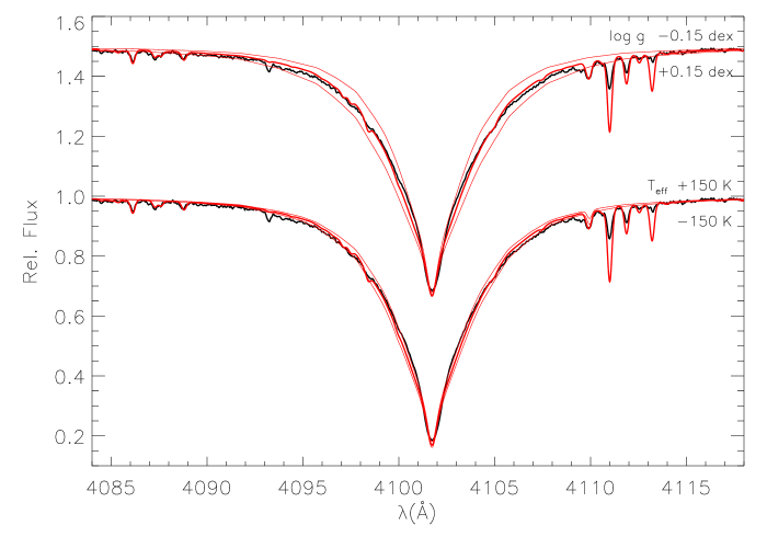
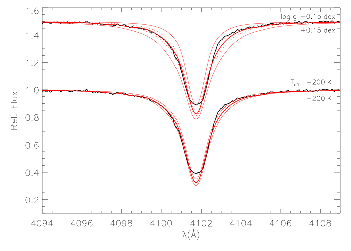
Figure 8: Impact of stellar parameter variations on non-LTE line profile fits for H$\delta$ in $\eta$ Leo (left) and HD 92207 (right). Spectrum synthesis for the adopted parameters (see Table 2, thick red line) and varied parameters, as indicated (thin lines), are compared to observation. A vertical shift by 0.5 units has been applied to the upper profiles. Note the decrease of the Balmer line strength in the progression from LC Ib ($\eta$ Leo) to Iae (HD 92207), and the increased sensitivity to the surface gravity parameter. In fact, the comparison indicates that for the more luminous supergiants uncertainties in the surface gravity determination become as low as 0.05 dex (dotted lines). The sensitivity to reasonable $T_{\rm eff}$-changes is almost negligible. Wind emission slightly contaminates the red wing of H$\delta$ in HD 92207.

Where it was once a supercomputing application, comprehensive non-LTE modelling like the present can now be made on workstations or PCs. Typical running times to achieve convergence in the statistical equilibrium and radiative transfer calculations with Detail range from $\sim$10 min for the most simple model atoms to a couple of hours for the Fe ii model on a 3 GHz P4 CPU – for one set of parameters. The formal solution for a total of 2–3 $\times$10${}^{5}$ frequency points with Surface requires $\sim$20–30 CPU min. Because of the highly iterative and interactive nature of our analysis procedure (see next two sections) the total time for a comprehensive study of one high-resolution, high-S/N spectrum, assuming excellent wavelength coverage from around the Balmer jump to $\sim$9 000 Å as typically achieved by modern Echelle spectrographs, amounts to 1–2 weeks for the experienced user. This is the price to pay for overcoming the restrictions of contemporary BA-SG abundance studies and advancing them from factor 2–3 accuracy astronomy to precision astrophysics.

Future extensions of the present work will aim to provide more non-LTE model atoms, but these quite often require the necessary atomic data to be calculated first, as many data are still unavailable in present-day literature. In particular, the status of collisional data has largely to be improved. Note that the Si ii ion in the silicon model atom by Becker & Butler (BeBu90) is only rudimentary (though sufficient for their main purpose, analyses of early B-stars). Several energy levels involved in the observed transitions in BA-SGs are missing, and test calculations indicate a wide spread of the non-LTE abundances from the remaining transitions. On the basis of these findings we refrain from using the model atom for analyses in the present work, but wish to emphasise that qualitatively the correct non-LTE behaviour – line strengthening – is predicted.

5 Determination of stellar parameters

Stellar parameter determination for BA-SGs is complicated because of the intrinsic variability of these objects. Observational data from different epochs may therefore reflect different physical states of the stellar atmosphere, unless these are obtained (nearly) simultaneously. While we can expect the mass of a supergiant and its surface abundances to be conserved on human timescales, other stellar parameters may not. The observed variability patterns of light curves, radial velocities and line profiles can be interpreted in favour of a mix of radial and non-radial pulsations (see e.g. Kaufer et al. Kauferetal97), which may affect $T_{\rm eff}$ and $\log g$, that in turn determine colours, the spectral energy distribution and the spectra. Even the stellar luminosity may be subject to small changes (Dorfi & Gautschy DoGa00). The parameter variations are not as pronounced as in other variable stars, but use of information from different epochs can potentially introduce systematic uncertainties into high-precision analyses. A solution is to derive the desired quantities from one set of observational data. Echelle spectra are the best choice, containing all information required for the derivation of stellar parameters and elemental abundances. With few exceptions, use of photometric data (from other sources) can thus be avoided. In the following we discuss the details of our spectroscopic approach for the parameter determination of BA-SGs. Spectrophotometry is only briefly considered for consistency checks. Finally, our findings are compared with previous analyses of the two well studied standards $\eta$ Leo and $\beta$ Ori.

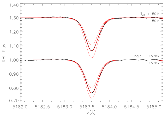
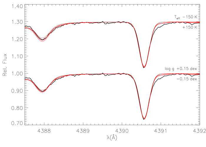
Figure 9: Temperature determination for $\eta$ Leo using the Mg i/ii non-LTE ionization equilibrium. Displayed are the observed line profiles for some of the strategic lines, Mg i $\lambda$ 5183 (left panel) and Mg ii $\lambda$ 4390 and He i $\lambda$ 4387 (right panel), and the best non-LTE fit for stellar parameters as given in Table 2 (thick red line); theoretical profiles for varied parameters are also shown (thin lines, as indicated). A vertical shift by 0.3 units has been applied to the upper set of profiles. Note the strong sensitivity of the minor ionic species, Mg i, to parameter changes, while Mg ii is virtually unaffected.

Figure 10: Fit diagrams of temperature- and gravity-sensitive indicators for $\eta$ Leo and $\beta$ Ori in the $T_{\rm eff}$–$\log g$-plane. The curves are parameterised by surface helium abundance $y$. The intersection determines $T_{\rm eff}$ and $\log g$, with uncertainties as indicated.

5.1 Spectroscopic indicators

The hydrogen lines are the most noticeable features in the spectra of BA-type stars. Their broadening by the linear Stark effect gives a sensitive surface gravity indicator in the mostly ionized atmospheric plasma. We employ the recent Stark broadening tables of Stehlé & Hutcheon (SH99, SH), which compare well with the classically used data from Vidal et al. (VCS73, VCS; with extensions of the grids by Schöning & Butler, private communication) in the BA-SG regime. The SH tables have not only the advantage of being based on the more sophisticated theory but they also cover the Paschen (and Lyman) series for transitions up to principal quantum number $n$ $=$ 30. A detailed discussion of our hydrogen non-LTE line-formation computations for BA-SGs can be found in Przybilla & Butler (PrBu04a), where lines of the Brackett and Pfund series were also studied. In short, it has been shown that except for the lower series members – which are affected or even dominated by the stellar wind – excellent consistency can be achieved from all available indicators, if accurate data for excitation via electron collisions are accounted for. Note that the only other study of H lines from these four series, in the prototype A-SG Deneb (Aufdenberg et al. Aufdenbergetal02), fails in this. Their non-LTE model atmosphere and line-formation computations produce much too strong near-IR features because of inaccurate collisional data in their hydrogen model atom, as indicated by our findings. The problems are resolved using the improved effective collision strengths (P. Hauschildt, private communication).

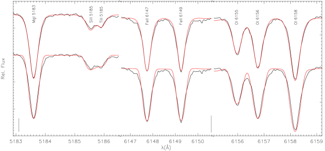
Figure 11: Determination of projected rotational and macroturbulent velocities, exemplarily shown for three spectral regions of $\eta$ Leo including discrete and blended absorption features. The upper comparison between observation (black line) and spectrum synthesis (red line, for finally derived mean abundances) is made for $\zeta$ $=$ 16.5 km s${}^{-1}$ and zero $v\,\sin i$ (our finally adopted optimum values), the lower comparison is made assuming a pure rotational profile with $v\,\sin i$ $=$ 13.3 km s${}^{-1}$. See the text for further discussion. Line identifiers are given. The markers are vertically extended by 0.05 units.

Our method for deriving surface gravities from the hydrogen lines deviates in a few details from the usual approach, which is based on the modelling of the H$\gamma$ and H$\delta$ line wings. The effect of variations of $\log g$ and $T_{\rm eff}$ on the H$\delta$ profiles of $\eta$ Leo and HD 92207 are displayed in Fig. 8. We have chosen parameter offsets to our finally adopted values which we consider conservative estimates for the uncertainties of our analysis. It is clear that the internal accuracy of our modelling is higher, amounting to $\lesssim$ 0.10 dex at LC Ib and as accurate as 0.05 dex at LC Iae. The temperature sensitivity is smaller, but non-negligible. Note the strong decrease of the H$\delta$ line strength in the luminosity progression. Close to the Eddington limit a modification by 0.05 dex in $\log g$ can amount to a change in $W_{\lambda}$ of the Balmer lines by 15%. Note also that in the less luminous supergiant not only the line wings but also the entire line profile and thus also the equivalent width is accurately reproduced (which becomes important for intermediate- and low-resolution studies), indicating that the model atmosphere is sufficiently realistic over all line-formation depths. At the highest luminosities the accuracy of the spectrum synthesis degrades somewhat, because of stellar wind and sphericity effects. However, excellent agreement can be restored even for the higher Balmer lines, and for the accessible Paschen series members (see Fig. 11 in Przybilla & Butler PrBu04a), which are formed even deeper in the atmosphere. This also includes good reproduction of the series limits and their transition into the continua. Moreover, we also account for the effects of non-solar helium abundances on the density structure (see Sect. 3.2), which is mandatory for achieving consistent results, but which has been ignored in all BA-SG analyses so far.

In order to resolve the ambiguity in $T_{\rm eff}/\log g$ another indicator has to be applied. In a spectroscopic approach this is typically the ionization equilibrium of one chemical species. Potential ionization equilibria useful for $T_{\rm eff}$ and $\log g$ determinations in optical/near-IR spectroscopy of BA-SGs are C i/ii, N i/ii, O i/ii, Mg i/ii, Al i/ii, Al ii/iii, Si ii/iii, S ii/iii, Fe i/ii and Fe ii/iii. Of these we can use only half because model atoms are currently unavailable for the rest. The lines of the minor ionic species are highly sensitive to temperature and electron density changes, while the weak lines of the major ionic species are excellent abundance indicators. A suitable set of parameters $T_{\rm eff}/\log g$ is found in the case where both ionic species indicate the same elemental abundance within the individual error margins. However, great care has to be practised in the modelling, using carefully selected model atmospheres (see Sect. 3) and sophisticated non-LTE techniques (see Sects. 4 and LABEL:sectabus).

An example is displayed in Fig. 9, where tests on the Mg i/ii ionization balance in one of the sample objects are performed. Results from the best fit obtained in the detailed non-LTE analysis are compared with those from conservative parameter studies at an unchanged elemental abundance. The sensitivity of the predicted Mg i line strengths to changes of $T_{\rm eff}$ and $\log g$ within the error margins is high, indicating internal uncertainties of $\Delta T_{\rm eff}$ $<$ 100 K and of $\Delta\log g$ $\lesssim$ 0.10 dex. The profile changes by conservative parameter variation are similar to those achieved by abundance variations of the order 0.1 dex. On the other hand, no perceptible changes are seen in the Mg ii line for the same parameter variations. All Mg i/ii lines behave in a similar way, and the same qualitative characteristics are shared with ionization equilibria from other elements.

Both, hydrogen profiles and ionization equilibria are affected by the helium abundance, which therefore has to be simultaneously constrained as an additional parameter. Enhanced helium abundances manifest in broadened hydrogen lines and shifts in ionization equilibria – in BA-SGs the spectral lines of the minor ionization species are strengthened. Thus, parameter studies assuming a solar helium abundance will tend to derive systematically higher effective temperatures and surface gravities. In the BA-SGs the transitions of He i are typically weak. The helium abundance $y$ (by number) can therefore be inferred from line profile fits to all available features. Typical uncertainties in the determination of stellar helium abundances amount to $\sim$10% because of the availability of excellent atomic data.

The whole process of the basic atmospheric parameter determination can be summarised in an $T_{\rm eff}$–$\log g$ diagram, which is done exemplarily for $\eta$ Leo and $\beta$ Ori in Fig. 10. The intersection of the different loci marks the appropriate set of stellar parameters. Note that these diagnostic diagrams differ from those typically found in the literature in two respects: first, the different indicators lead to consistent stellar parameters, and second, the loci are parameterised with the helium abundance, a necessary procedure to obtain the excellent agreement. When deriving the stellar parameters one can profit from the slow and rather predictable behaviour of the derived helium abundance with varying $T_{\rm eff}$/$\log g$.

The microturbulent velocity $\xi$ is determined in the usual way by forcing elemental abundances to be independent of equivalent widths. The difference to previous studies of BA-SGs is that this is done on the basis of non-LTE line-formation (see Fig. LABEL:nlteabus and the discussion in Sect. LABEL:sectabus). An LTE analysis would tend to find higher values in order to compensate non-LTE line strengthening. Typically, the extensive iron spectrum is used for the microturbulence analysis. Because the Fe ii non-LTE computations are by far the most time-intensive, alternatives have to be considered here. The Ti ii and in particular the N i spectra are excellent replacements, the latter distinguished by more accurate atomic data. Later, the iron lines can be used to verify the $\xi$-determination. Note that this is the only occasion where equivalent widths are used in the analysis process – elsewhere line profile fits are preferred.

Table 2: Basic properties and stellar parameters of the sample stars

	HD 87737		HD 111613		HD 92207		HD 34085
Name	$\eta$ Leo		…		…		$\beta$ Ori, Rigel
Association${}^{\rm a}$	Field		Cen OB1		Car OB1		Ori OB1
Spectral Type${}^{\rm b}$	A0 Ib		A2 Iabe		A0 Iae		B8 Iae:
$\alpha$ (J2000)${}^{\rm b}$	10 07 19.95		12 51 17.98		10 37 27.07		05 14 32.27
$\delta$ (J2000)${}^{\rm b}$	$+$16 45 45.6		$-$60 19 47.2		$-$58 44 00.0		$-$08 12 05.9
$l\,(\degr)$${}^{\rm b}$	219.53		302.91		286.29		209.24
$b\,(\degr)$${}^{\rm b}$	$+$50.75		+2.54		$-$0.26		$-$25.25
$\pi$ (mas)${}^{\rm c}$	1.53$\pm$	0.77	1.09$\pm$	0.62	0.40$\pm$	0.53	4.22$\pm$	0.81
$d$ (pc)${}^{\rm d}$	630$\pm$	90	2 290$\pm$	220	3 020$\pm$	290	360$\pm$	40
$R_{\rm g}\,(\mbox{kpc})$	8.25$\pm$	0.83	6.97$\pm$	0.84	7.66$\pm$	0.77	8.23$\pm$	0.82
$\theta_{\rm D}$ (mas)${}^{\rm e}$	…		…		…		2.55$\pm$	0.05
$v_{\mathrm{rad}}\,(\mbox{km\,s}^{-1})$${}^{\rm b}$	$+$3.3$\pm$	0.9	$-$21.0$\pm$	2.0	$-$8.5$\pm$	5.0	$+$20.7$\pm$	0.9
$\mu_{\alpha}$ (mas yr${}^{-1}$)${}^{\rm c}$	$-$1.94$\pm$	0.92	$-$5.26$\pm$	0.55	$-$7.46$\pm$	0.53	1.87$\pm$	0.77
$\mu_{\delta}$ (mas yr${}^{-1}$)${}^{\rm c}$	$-$0.53$\pm$	0.43	$-$1.09$\pm$	0.39	3.11$\pm$	0.44	$-$0.56$\pm$	0.49
$U\,(\mbox{km\,s}^{-1})$	4		$-$49		$-$103		$-6$
$V\,(\mbox{km\,s}^{-1})$	222		211		201		214
$W\,(\mbox{km\,s}^{-1})$	6		$-$6		$-$6		1
Atmospheric:
$T_{\mathrm{eff}}$ (K)	9 600$\pm$	150	9 150$\pm$	150	9 500$\pm$	200	12 000$\pm$	200
$\log g$ (cgs)	2.00$\pm$	0.15	1.45$\pm$	0.10	1.20$\pm$	0.10	1.75$\pm$	0.10
$y$	0.13$\pm$	0.02	0.105$\pm$	0.02	0.12$\pm$	0.02	0.135$\pm$	0.02
$[$M/H$]$ (dex)	$-$0.04$\pm$	0.03	$-$0.11$\pm$	0.03	$-$0.09$\pm$	0.07	$-$0.06$\pm$	0.10
$\xi\,(\mbox{km\,s}^{-1})$	4$\pm$	1	7$\pm$	1	8$\pm$	1	7$\pm$	1
$\zeta\,(\mbox{km\,s}^{-1})$	16$\pm$	2	21$\pm$	3	20$\pm$	5	22$\pm$	5
$v\sin i\,(\mbox{km\,s}^{-1})$	0$\pm$	3	19$\pm$	3	30$\pm$	5	36$\pm$	5
Photometric:
$V$ (mag)${}^{\rm f}$	3.52		5.72		5.45		0.12
$B-V^{\rm f}$	$-$0.03		+0.38		+0.50		$-$0.03
$U-B^{\rm f}$	$-$0.21		$-$0.10		$-$0.24		$-$0.66
$E(B-V)$	0.02		0.39		0.48${}^{\rm g}$		0.05
$(m-M)_{0}^{\rm d}$	9.0$\pm$	0.3	11.8$\pm$	0.2	12.4$\pm$	0.2	7.8$\pm$	0.2
$M_{V}$	$-$5.54$\pm$	0.3	$-$7.29$\pm$	0.2	$-$8.82$\pm$	0.2	$-$7.84$\pm$	0.2
$B.C.$	$-$0.29		$-$0.23		$-$0.34		$-$0.78
$M_{\mathrm{bol}}$	$-$5.83$\pm$	0.3	$-$7.52$\pm$	0.2	$-$9.16$\pm$	0.2	$-$8.62$\pm$	0.2
Physical:
$\log L/$L${}_{\odot}$	4.23$\pm$	0.12	4.90$\pm$	0.08	5.56$\pm$	0.08	5.34$\pm$	0.08
$R/$R${}_{\odot}$	47$\pm$	8	112$\pm$	12	223$\pm$	24	109$\pm$	12
$M/$M${}_{\odot}^{\rm ZAMS}$	10$\pm$	1	16$\pm$	1	30$\pm$	3	24$\pm$	3
$M/$M${}_{\odot}^{\rm evol}$	10$\pm$	1	15$\pm$	1	25$\pm$	3	21$\pm$	3
$M/$M${}_{\odot}^{\rm spec}$	8$\pm$	4	13$\pm$	4	29$\pm$	10	24$\pm$	8
$\tau_{\rm evol}$ (Myr)	25$\pm$	5	14$\pm$	2	7$\pm$	1	8$\pm$	1

${}^{\rm a}$ Blaha & Humphreys (BlHu89)   ${}^{\rm b}$ adopted from the Simbad database at CDS   ${}^{\rm c}$ Perryman et al. (Perrymanetal97)   ${}^{\rm d}$ see text   ${}^{\rm e}$ Hanbury Brown et al. (HanburyBrownetal74)   ${}^{\rm f}$ Nicolet (Nicolet78)   ${}^{\rm g}$ with $R_{V}$ $=$ 3.9, see Sect. 5.3

Good starting estimates for the microturbulent velocity in BA-SGs are $\xi$ $=$ 4, 6 and 8 km s${}^{-1}$ for objects of LC Ib, Iab and Ia, respectively. After the determination of an improved value of $\xi$ the model atmosphere has to be recalculated in some cases, and small corrections to $T_{\rm eff}$/$\log g$/$y$ may become applicable. Only one iteration step is typically necessary to reestablish consistency in the atmospheric parameters. The uncertainties amount to typically $\pm$1 km s${}^{-1}$. In the present study the different microturbulence indicators give a single value for $\xi$ within these error margins. This is consistent with findings from recent (LTE) work on less-luminous A-type supergiants (Venn Venn95a, Venn99), while older studies based on more simple model atmospheres and less accurate oscillator strengths had to invoke different values for various elemental species, or a depth-dependent $\xi$ (e.g. Rosendhal Rosendhal70; Aydin Aydin72).

Microturbulence also has to be considered as additional non-thermal broadening agent in the radiative transfer and statistical equilibrium computations. The Doppler width is then given by $\Delta\lambda_{\rm D}=\lambda_{0}/c\,(v_{\rm th}^{2}+\xi^{2})^{1/2}$, where $\lambda_{0}$ is the rest wavelength of the transition, $c$ the speed of light and $v_{\rm th}$ the thermal velocity of the chemical species of interest. The main effect is a broadening of the frequency bandwidth for absorption in association with a shift in line-formation depth, typically leading to a net strengthening of individual lines by different amounts, see e.g. Przybilla et al. (Przybillaetal00; Przybillaetal01a; Przybillaetal01b) for further details.

Individual metal abundances are typically of secondary importance for the computation of model atmospheres, as elemental ratios are remarkably constant (i.e. close to solar) over a wide variety of stars, except for the chemically peculiar. We determine the stellar metallicity $[$M/H$]$, which is the more important parameter, as the arithmetic mean from five elements, for which non-LTE computations can be done and which are unaffected by mixing processes: $[{\rm M/H}]\equiv([{\rm O/H}]+[{\rm Mg/H}]+[{\rm S/H}]+[{\rm Ti/H}]+[{\rm Fe/H}])/5$. High weight is thus given to the $\alpha$–process elements, which have a different nucleosynthesis history than the iron group elements, but $[\alpha$/Fe$]$ $\sim$ 0 can be expected for these Population I objects. Because of the importance of metallicity for line blanketing a further iteration step may be required in the parameter determination.

Finally, the projected rotational velocity $v\sin i$ and the (radial-tangential) macroturbulent velocity $\zeta$ are derived from a comparison of observed line profiles with the spectrum synthesis. Single transitions as well as line blends should be used for this, as they contain some complementary information. Both quantities are treated as free parameters to obtain a best fit via convolution of the synthetic profile with rotation and macroturbulence profiles (Gray Gray92a), while also accounting for a Gaussian instrumental profile. An example is shown in Fig. 11, where the comparison with observation indicates pure macroturbulence broadening for $\eta$ Leo. The theoretical profiles intersect the observed profiles if the spectral lines are broadened by rotation alone, resulting in slightly too broad line cores and insufficiently broad line wings. Typically, both parameters are non-zero, with the macroturbulent velocity amounting to less than twice the sonic velocity in the atmospheric plasma. Macroturbulence is suggested to be related to surface motions caused by (high-order) nonradial oscillations (Lucy Lucy76). Weak lines should be used for the $v\sin i$ and $\zeta$-determinations in supergiants in order to avoid systematic uncertainties due to asymmetries introduced by the outflowing velocity field in the strong lines.

5.2 Stellar parameters of the sample objects

We summarise the basic properties and derived stellar parameters of the sample supergiants in Table 2. The first block of information concentrates on quantities which in principle can be deduced directly, with only little modelling involved. Besides Henry-Draper catalogue numbers, alternative names, information on association membership and spectral classification and equatorial and galactic coordinates are given. Hipparcos parallaxes $\pi$ have been included for completeness, as none of the measurements is of sufficient statistical significance. The stellar distances $d$ are therefore deduced by other means.

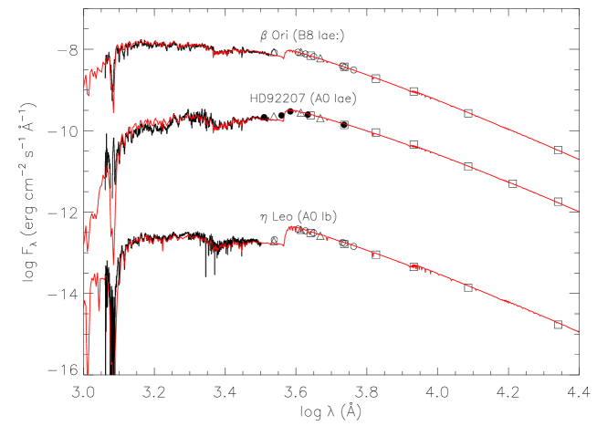
Figure 12: Computed (red full lines) and measured spectral energy distributions for the sample stars from the UV to the near-IR in the $K$-band. Overall, good to excellent agreement is obtained. Displayed are IUE spectrophotometry (full lines), Johnson (boxes), Strömgren (triangles), Walraven (filled circles) and Geneva photometry (open circles). The observations have been dereddened using colour excesses according to Table 2. A ratio $R_{V}$ $=$$A_{V}/E(B-V)$ $=$ 3.1, as typical for the local ISM, is assumed for $\beta$ Ori and $\eta$ Leo. In the case of the notably reddened HD 92207 both, color excess and $R_{V}$, can be determined, implying $R_{V}$ $=$ 3.9. For clarity, the data for $\eta$ Leo has been shifted vertically by $-$3 units. IUE spectrophotometry for HD 111613 is not available. Consequently, this star has been omitted from the comparison.

A distance modulus of 8$\aas@@fstack{m}$5 (viz. 500 pc) is found for the Ori OB 1 association by Blaha & Humphreys (BlHu89). However, $\beta$ Ori shows a smaller radial velocity than the mean of the Ori OB1 association ($\sim$30 km s${}^{-1}$). Therefore, the association distance gives only an upper limit, if one assumes that the star was formed near the centre of Ori OB1. During its lifetime $\beta$ Ori could have moved $\sim$100 pc from its formation site. The finally adopted distance of 360 pc is indicated by Hoffleit & Jaschek (HoJa82), who associate $\beta$ Ori with the $\tau$ Ori R1 complex.

Recent studies of the cluster NGC 4755 found a distance modulus of 11.6$\pm$0.2 mag, with a mean value of $E(B$ $-$ $V)$ of 0.41$\pm$0.05 mag (Sagar & Cannon SaCa95) and 0.36 $\pm$0.02 mag (Sanner et al. Sanneretal01). However, HD 111613 is situated at a rather large distance from the cluster centre and was not observed in either study. In a previous work (Dachs & Kaiser DaKa84) the object was found to be slightly behind the cluster by 0.2 mag. Consequently, this difference is accounted for in the present study, otherwise using the modern distance.

The line of sight towards the Car OB1 association coincides with a Galactic spiral arm, such that the star population in Car OB1 is distributed in depth over 2 to 3 kpc (Shobbrook & Lyngå ShLy94). A more decisive constraint on the distance of HD 92207 is indicated by Carraro et al. (Carraroetal01), who argue that the star may be associated with the cluster NGC 3324. The star will not be gravitationally bound because of its large proper motion, but appears to be spatially close to the cluster, and may have been ejected. We therefore adopt the cluster distance modulus for HD 92207 with an increased error margin. Finally, the distance to the field star $\eta$ Leo can only be estimated, based on its spectroscopic parallax.

Galactocentric distances of the stars are calculated from the coordinates and $d$, using a galactocentric solar distance of $R_{0}$ $=$ 7.94$\pm$0.42 kpc (Eisenhauer et al. Eisenhaueretal03). In one case an interferometrically determined true angular diameter $\theta_{\rm D}$ (allowing for limb darkening) is available from the literature. Our measured radial velocities $v_{\rm rad}$ (from cross-correlation with synthetic spectra) are compatible with the literature values, which in combination with proper motions $\mu_{\alpha}$ and $\mu_{\delta}$ are used to calculate galactocentric velocities $U$, $V$ and $W$, assuming standard values for the solar motion ($U$ $=$ 10.00 km s${}^{-1}$, $V$ $=$ 5.23 km s${}^{-1}$, $W$ $=$ 7.17 km s${}^{-1}$, Dehnen & Binney DeBi98) relative to the local standard of rest (220 km s${}^{-1}$, Kerr & Lynden-Bell KeLy86).

In the second block our results from the spectroscopic stellar parameter determination are summarised. Photometric data are collected in the third block. Observed visual magnitudes and colours in the Johnson system are used to derive the colour excess $E(B-V)$ by comparison with synthetic colours. Note that for HD 111613 and HD 92207 the derived colour excess is in excellent agreement with literature values for their parent clusters. From the distance moduli $(m-M)_{0}$ absolute visual magnitudes $M_{V}$ are calculated, which are transferred to absolute bolometric magnitudes $M_{\mathrm{bol}}$ by application of bolometric corrections $B.C.$ from the model atmosphere computations. Note also our previous comments on the photometric variability of BA-SGs, which can introduce some systematic uncertainty into our analysis, as the photometry and our spectra may reflect slightly different physical states of the stellar atmospheres. The sensitivity of the Johnson colours to $T_{\rm eff}$-changes is not high enough to use them as an alternative indicator for a precise determination of the stellar effective temperature.

Finally, we derive the physical parameters luminosity $L$, stellar radius $R$ and spectroscopic mass $M^{\rm spec}$ of the sample stars by combining atmospheric parameters and photometry. Thus the determined stellar radius of $\beta$ Ori is in good agreement with that derived from the angular diameter measurement (99$\pm$11 R${}_{\odot}$). From comparison with stellar evolution computations (Meynet & Maeder MeMa03) zero-age main-sequence masses $M^{\rm ZAMS}$ and evolutionary masses $M^{\rm evol}$ are determined, and the evolutionary age $\tau_{\rm evol}$. The stars were of early-B and late-O spectral type on the main sequence. The results will be discussed in detail in Sect. LABEL:sectevol. Note that the rather large uncertainties in the distance determination dominate the error budget of the physical parameters.

Table 3: Comparison of stellar parameters of $\eta$ Leo and $\beta$ Ori from the literature

Source	$T_{\rm eff}$ (K)		$\log g$ (cgs)		$\xi$ (km s${}^{-1}$)		Method	Notes
HD 87737
This work	9 600$\pm$	150	2.00$\pm$	0.15	4$\pm$	1	NLTE H i, N i/ii, Mg i/ii, (C i/ii),	…
							spectrophotometry
Venn (Venn95a)	9 700$\pm$	200	2.0$\pm$	0.2	4$\pm$	1	H$\gamma$, NLTE Mg i/ii	Kurucz (Kurucz93) atmospheres
Lobel et al. (Lobeletal92)	10 200$\pm$	370	1.9$\pm$	0.4	5.4$\pm$	0.7	LTE Fe i/ii	Kurucz (Kurucz79) atmospheres,
								equivalent widths from Wolf (Wolf71)
Lambert et al. (Lambertetal88)	10 500		2.2		…		Strömgren photometry $+$ H$\beta$	Kurucz (Kurucz79) atmospheres
Wolf (Wolf71)	10 400$\pm$	300	2.05$\pm$	0.20	2…10		Balmer lines, Balmer jump,	early LTE atmospheres, no line-
							LTE Mg i/ii, Fe i/ii	blanketing, photographic spectra
HD 34085
This work	12 000$\pm$	200	1.75$\pm$	0.10	7$\pm$	1	NLTE H i, N i/ii, O i/ii, S ii/iii,	…
							spectrophotometry
McErlean et al. (McErleanetal99)	13 000$\pm$	1 000	1.75$\pm$	0.2	10		NLTE H$\gamma$, H$\delta$, Si ii/iii	Hubeny (Hubeny88) H$+$He NLTE models,
								no line-blanketing
Israelian et al. (Israelianetal97)	13 000$\pm$	500	1.6$\pm$	0.1	7		NLTE H$\gamma$, H$\delta$, Si	Hubeny (Hubeny88) H$+$He NLTE models,
								no line-blanketing
Takeda (Takeda94)	13 000$\pm$	500	2.0$\pm$	0.3	7		LTE H$\gamma$, H$\delta$, spectrophotometry	Kurucz (Kurucz79) atmospheres
Stalio et al. (Stalioetal77)	12 070$\pm$	160	…		…		angular diameter, total flux	early line-blanketed LTE atmospheres

5.3 Spectrophotometry

The principal aim of the present study is a self-consistent method for the analysis of BA-type supergiants in the whole. This requires above all the reproduction of the stellar spectral energy distribution (SED). A comparison of our model fluxes for three of the sample supergiants with observation is made in Fig. 12. The observational database consists of IUE spectrophotometry (as obtained from the IUE Final Archive) and photometry in several passbands (broad-band to small-band) from the near-UV to near-IR, in the Johnson (Morel & Magnenat MoMa78; Ducati Ducati02, for HD 92207), Geneva (Rufener Rufener88), Strömgren (Hauck & Mermilliod HaMe98) and Walraven systems (de Geus et al. deGeusetal90). We have omitted HD 111613 from the comparison because crucial UV spectrophotometry is unavailable for this star. The observations have been de-reddened using a reddening law according to Cardelli et al. (Cardellietal89). Overall, good to excellent agreement is found. This verifies our spectroscopic stellar parameter determination.

Use of SED information can provide an additional $T_{\rm eff}$-indicator, independent of weak spectral lines used in the ionization equilibria approach. This makes SED-fitting attractive for extragalactic applications, as it has the potential to improve on the modelling situation when only intermediate-resolution spectra are available (see Sect. LABEL:sectmedres). As the present work concentrates on the spectroscopic approach to BA-SGs analyses, we will report on a detailed investigation of this elsewhere.

5.4 Comparison with previous analyses

The two MK standards $\eta$ Leo and $\beta$ Ori have been analysed with model atmosphere techniques before. A comparison of our derived stellar parameters with literature values is made in Table 3. The methods used for the parameter determination are indicated and comments on the model atmospheres and the observational data are given. For the comparison we have omitted publications earlier than the 1970ies.

Good agreement of the present parameters for $\eta$ Leo with those of Venn (Venn95a) is found, as the methods employed are comparable. Other authors find a substantially hotter $T_{\rm eff}$ for this star, while the values for surface gravity and microturbulence are comparable. All these values are based on less elaborate model atmospheres, with less or no line-blanketing, and they completely ignore non-LTE effects on the line formation. Note that a $T_{\rm eff}$ of 9380 K is obtained from Strömgren photometry, using the calibration of Gray (Gray92b).

For $\beta$ Ori basically two disjunct values for the effective temperature are found in the literature. Model atmosphere analyses so far found a systematically higher $T_{\rm eff}$, which is likely to be due in good part to ignored/reduced line-blanketing. The measurements of surface gravity and microturbulent velocity are again similar. The other group of $T_{\rm eff}$ analyses mostly find significantly lower values than that derived in the present work, from measured total fluxes and interferometric radius determinations, or from the infrared flux method: 11 800 $\pm$ 300/11 700 $\pm$ 200 (Nandy & Schmidt NaSch75), 11 550 $\pm$ 170 (Code et al. Codeetal76), 11 410 $\pm$ 330 (Beeckmans Beeckmans77), 11 780 (Underhill et al. Underhilletal79), 11 014 (Blackwell et al. Blackwelletal80), 11 380 (Underhill & Doazan UnDo82) and 11 023/11 453 K (Glushneva Glushneva85). These methods are prone to systematic errors from inappropriate corrections for interstellar absorption. The authors all supposed zero interstellar extinction. In fact, the only such study that accounts for a non-zero $E(B-V)$ (Stalio et al. Stalioetal77, $+$0.04 vs. $+$0.05 as derived here) finds a temperature in excellent agreement with the present value, see Table 3. However, using LTE Fe ii/iii and Si ii/iii ionization equilibria and Balmer profiles they derive $T_{\rm eff}$ $\gtrsim$ 13 000 K.

Element Sun${}^{\mathrm{a}}$ $\eta\,$Leo HD 111613 HD 92207 $\beta$ Ori Gal AI${}^{\mathrm{b}}$ Gal BV${}^{\mathrm{c}}$ Gal BV${}^{\mathrm{d}}$ Gal BV${}^{\mathrm{e}}$ Gal BV${}^{\mathrm{f}}$ He i 10.99$\pm$ 0.02 11.18$\pm$ 0.04 (14) 11.07$\pm$ 0.05 (10) 11.14$\pm$ 0.04 (10) 11.19$\pm$ 0.04 (15) … … 11.13$\pm$ 0.22 11.05$\pm$ 0.10 … C i 8.52$\pm$ 0.06 7.94$\pm$ 0.10 (4) 8.10$\pm$ 0.07 (2) … … 8.14$\pm$ 0.13 … … … … C ii 8.52$\pm$ 0.06 8.10$\pm$ 0.09 (3) 8.24$\pm$ 0.06 (3) 8.33 (1) 8.15$\pm$ 0.05 (3) … 8.27$\pm$ 0.13 8.20$\pm$ 0.10 8.22$\pm$ 0.15 7.87$\pm$ 0.16 N i 7.92$\pm$ 0.06 8.41$\pm$ 0.09 (20) 8.40$\pm$ 0.10 (16) 8.25$\pm$ 0.04 (11) 8.50$\pm$ 0.07 (11) 8.37$\pm$ 0.21${}^{*}$ … … … … N ii 7.92$\pm$ 0.06 8.32 (1) 8.36 (1) 8.28 (1) 8.51$\pm$ 0.06 (16) … 7.63$\pm$ 0.15 7.75$\pm$ 0.27 7.78$\pm$ 0.27 7.90$\pm$ 0.22 O i 8.83$\pm$ 0.06 8.78$\pm$ 0.05 (13) 8.70$\pm$ 0.04 (9) 8.79$\pm$ 0.07 (6) 8.78$\pm$ 0.04 (6) 8.77$\pm$ 0.12 … … … … O ii 8.83$\pm$ 0.06 … … … 8.83$\pm$ 0.03 (5) … 8.55$\pm$ 0.14 8.64$\pm$ 0.20 8.52$\pm$ 0.16 8.89$\pm$ 0.14 Ne i 8.08$\pm$ 0.06 8.39$\pm$ 0.07 (7) 8.42$\pm$ 0.06 (5) 8.50$\pm$ 0.14 (7) 8.40$\pm$ 0.08 (9) … … … 8.10$\pm$ 0.05${}^{**}$ … Mg i 7.58$\pm$ 0.01 7.52$\pm$ 0.08 (7) 7.46$\pm$ 0.04 (4) 7.60$\pm$ 0.04 (4) … 7.48$\pm$ 0.17 … … … … Mg ii 7.58$\pm$ 0.01 7.53$\pm$ 0.04 (12) 7.43$\pm$ 0.04 (6) 7.40$\pm$ 0.05 (5) 7.42$\pm$ 0.02 (4) 7.46$\pm$ 0.17 7.42$\pm$ 0.22 7.59$\pm$ 0.22 7.38$\pm$ 0.12 7.70$\pm$ 0.34 Al i 6.49$\pm$ 0.01 6.11$\pm$ 0.06 (2) 6.06$\pm$ 0.06 (2) … … … … … … … Al ii 6.49$\pm$ 0.01 6.39$\pm$ 0.17 (5) 6.55$\pm$ 0.27 (6) 6.38$\pm$ 0.38 (6) 6.14$\pm$ 0.08 (4) … … … … … Al iii 6.49$\pm$ 0.01 … … … 7.00$\pm$ 0.38 (4) … 6.08$\pm$ 0.12 6.21$\pm$ 0.19 6.12$\pm$ 0.18 6.31$\pm$ 0.15 Si ii 7.56$\pm$ 0.01 7.58$\pm$ 0.19 (4) 7.45$\pm$ 0.29 (3) 7.33$\pm$ 0.05 (2) 7.27$\pm$ 0.13 (3) 7.33$\pm$ 0.17 … 7.42$\pm$ 0.23 7.19$\pm$ 0.21 … Si iii 7.56$\pm$ 0.01 … … … 8.13$\pm$ 0.23 (3) … 7.26$\pm$ 0.19 7.42$\pm$ 0.23 7.19$\pm$ 0.21 7.50$\pm$ 0.15 P ii 5.56$\pm$ 0.06 … … … 5.53$\pm$ 0.06 (4) … … … … … S ii 7.20$\pm$ 0.06 7.15$\pm$ 0.07 (14) 7.07$\pm$ 0.08 (10) 7.12$\pm$ 0.08 (16) 7.05$\pm$ 0.09 (26) … … … … … S iii 7.20$\pm$ 0.06 … … … 7.08$\pm$ 0.04 (2) … 7.24$\pm$ 0.14 … 6.87$\pm$ 0.26 … Ca ii 6.35$\pm$ 0.01 6.31 (1) … … … … … … … … Sc ii 3.10$\pm$ 0.01 2.57$\pm$ 0.14 (3) 2.64$\pm$ 0.27 (2) 2.42 (1) … 3.13$\pm$ 0.20 … … … … Ti ii 4.94$\pm$ 0.02 4.89$\pm$ 0.13 (29) 4.86$\pm$ 0.12 (25) 4.87$\pm$ 0.09 (15) 5.01$\pm$ 0.07 (4) 4.86$\pm$ 0.25 … … … … V ii 4.02$\pm$ 0.02 3.57$\pm$ 0.06 (6) 3.63$\pm$ 0.08 (6) 3.55$\pm$ 0.04 (3) … … … … … … Cr ii 5.69$\pm$ 0.01 5.62$\pm$ 0.08 (29) 5.55$\pm$ 0.08 (24) 5.28$\pm$ 0.08 (21) 5.42$\pm$ 0.11 (8) 5.61$\pm$ 0.23 … … … … Mn ii 5.53$\pm$ 0.01 5.38$\pm$ 0.02 (7) 5.36$\pm$ 0.04 (6) 5.24 (1) 5.33 (1) 5.81$\pm$ 0.20 … … … … Fe i 7.50$\pm$ 0.01 7.34$\pm$ 0.12 (21) 7.37$\pm$ 0.10 (13) … … 7.56$\pm$ 0.24 … … … … Fe ii 7.50$\pm$ 0.01 7.52$\pm$ 0.09 (35) 7.42$\pm$ 0.05 (35) 7.34$\pm$ 0.07 (24) 7.47$\pm$ 0.08 (20) 7.40$\pm$ 0.11 … … … … Fe iii 7.50$\pm$ 0.01 … … … 7.45$\pm$ 0.07 (10) … … … 7.36$\pm$ 0.20 … Ni ii 6.25$\pm$ 0.01 6.30$\pm$ 0.06 (7) 6.17$\pm$ 0.04 (7) 6.00$\pm$ 0.01 (2) 5.91$\pm$ 0.08 (4) … … … … … Sr ii 2.92$\pm$ 0.02 2.37$\pm$ 0.04 (2) 2.41$\pm$ 0.03 (2) 2.49$\pm$ 0.04 (2) … 2.41$\pm$ 0.21 … … … … Ba ii 2.22$\pm$ 0.02 2.00 (1) 2.13 (1) … … … … … … …
${}^{\mathrm{a}}$ Grevesse & Sauval (GrSa98): meteoritic abundances for non-volatile elements;   ${}^{\mathrm{b}}$ Venn (Venn95a, Venn95b);   ${}^{\mathrm{c}}$ Daflon & Cunha (DaCu04): mean values of stars from 17 clusters/associations at $R_{0}$ $\pm$2 kpc;   ${}^{\mathrm{d}}$ Gummersbach et al. (Gummersbachetal98): mean values of 10 stars at $R_{0}$ $\pm$2 kpc;   ${}^{\mathrm{e}}$ mean from Kilian (Kilian92, Kilian94);   ${}^{\mathrm{f}}$ Rolleston et al. (Rollestonetal00): mean of stars from 11 clusters/associations at $R_{0}$ $\pm$2 kpc; ${}^{\mathrm{*}}$ reanalysis by Venn & Przybilla (VePr03) – result from Venn (Venn95b): 8.05$\pm$0.19;   ${}^{\mathrm{**}}$ Ne ii

Table 4: Elemental abundances in the sample stars