Forced oscillations in a hydrodynamical accretion disk and QPOs.

Abstract

This is the second of a series of papers aimed to look for an explanation on the generation of high frequency quasi-periodic oscillations (QPOs) in accretion disks around neutron star, black hole, and white dwarf binaries. The model is inspired by the general idea of a resonance mechanism in the accretion disk oscillations as was already pointed out by Abramowicz & Kluźniak (Abramowicz2001 (2001)). In a first paper (Pétri 2005a , paper I), we showed that a rotating misaligned magnetic field of a neutron star gives rise to some resonances close to the inner edge of the accretion disk. In this second paper, we suggest that this process does also exist for an asymmetry in the gravitational potential of the compact object. We prove that the same physics applies, at least in the linear stage of the response to the disturbance in the system. This kind of asymmetry is well suited for neutron stars or white dwarfs possessing an inhomogeneous interior allowing for a deviation from a perfectly spherically symmetric gravitational field. After a discussion on the magnitude of this deformation applied to neutron stars, we show by a linear analysis that the disk initially in a cylindrically symmetric stationary state is subject to three kinds of resonances: a corotation resonance, a Lindblad resonance due to a driven force and a parametric resonance. In a second part, we focus on the linear response of a thin accretion disk in the 2D limit. Waves are launched at the aforementioned resonance positions and propagate in some permitted regions inside the disk, according to the dispersion relation obtained by a WKB analysis. In a last part, these results are confirmed and extended via non linear hydrodynamical numerical simulations performed with a pseudo-spectral code solving Euler’s equations in a 2D cylindrical coordinate frame. We found that for a weak potential perturbation, the Lindblad resonance is the only effective mechanism producing a significant density fluctuation. In a last step, we replaced the Newtonian potential by the so called logarithmically modified pseudo-Newtonian potential in order to take into account some general-relativistic effects like the innermost stable circular orbit (ISCO). The latter potential is better suited to describe the close vicinity of a neutron star or a black hole. However, from a qualitative point of view, the resonance conditions remain the same. The highest kHz QPOs are then interpreted as the orbital frequency of the disk at locations where the response to the resonances are maximal. It is also found that strong gravity is not required to excite the resonances.

1 INTRODUCTION

Accretion disks a very commonly encountered in the astrophysical context. In the case where the accreting star is a compact object, they offer a very efficient way to release the gravitational energy into X-ray emission. However the process of release of angular momentum leading to the accretion is still poorly understood. The discovery of the high frequency quasi-periodic oscillations (kHz-QPOs) in the Low Mass X-ray Binaries (LMXBs) in 1996 offers a new tool for the diagnostic of the physics in the innermost part of an accretion disk and therefore in a strong gravitational field.

To date, quasi-periodic oscillations have been observed in about twenty LMXBs sources containing an accreting neutron star. Among these systems, the high-frequency QPOs (kHz-QPOs) which mainly show up by pairs, possess strong similarities in their frequencies, ranging from 300 Hz to about 1300 Hz, and in their shape (see van der Klis vanderKlis2000 (2000) for a review).

Since this first discovery several models have been proposed to explain the kHz-QPOs phenomenon observed in LMXBs. A beat-frequency model was introduced to explain the commensurability between the twin kHz-QPOs frequency difference and the neutron star rotation. This interaction between the orbital motion and the star rotation happens at some preferred radius. Alpar & Shaham (Alpar1985 (1985)) and Shaham (Shaham1987 (1987)) proposed the magnetospheric radius to be the preferred radius leading to the magnetospheric beat-frequency model. The sonic-point beat-frequency model was suggested by Miller et al. (Miller1998 (1998)). In this model, the preferred radius is the point where the radial inflow becomes supersonic. But soon after, some new observations on Scorpius X-1 showed that the frequency difference is not constant (van der Klis et al. vanderKlis1997 (1997)). This was then confirmed in other LMXBs like 4U 1636-53 (Jonker et al. Jonker2002 (2002)). The sonic-point beat frequency model was then modified to take into account this new fact (Lamb & Miller Lamb2001 (2001)).

The relativistic precession model introduced by Stella & Vietri (Stella1998 (1998), Stella1999 (1999)) makes use of the motion of a single particle in the Kerr-spacetime. In this model, the kHz-QPOs frequency difference is related to the relativistic periastron precession of weakly elliptic orbits while the low-frequencies QPOs are interpreted as a consequence of the Lense-Thirring precession. Markovic & Lamb (Markovic1998 (1998)) have also suggested this precession in addition to some radiation warping torque which could explain the low frequency QPOs. More promisingly, Abramowicz & Kluźniak (Abramowicz2001 (2001)) introduced a resonance between orbital and epicyclic motion that can account for the 3:2 ratio around Kerr black holes leading to an estimate of their mass and spin. Indeed, for black hole candidates the 3:2 ratio was first noticed by Abramowicz & Kluźniak (Abramowicz2001 (2001)) who also recognized and stressed its importance. Abramowicz et al. (Abramowicz2003 (2003)) showed that the non-linear resonance for the geodesic motion of a test particle can lead to the 3:2 ratio for the two main resonances. Now the 3:2 ratio of black hole QPOs frequencies is well established (McClintock & Remillard, MacClintock2003 (2003)). Kluźniak et al. (2004a ) showed that the twin kHz-QPOs can be explained by a non linear resonance in the epicyclic motion of the accretion disk. The idea that a resonance in modes of accretion disk oscillations may be excited by a coupling to the neutron star spin is discussed by Kluźniak et al. (2004b ). Numerical simulations in which the disk was disturbed by an external periodic field confirmed this point of view (Lee et al. Lee2004 (2004)). Rebusco (Rebusco2004 (2004)) developed the analytical treatment of these oscillations. More recently, Török et al. (Torok2005 (2005)) applied this resonance to determine the spin of some microquasars. In other models, the QPOs are identified with gravity or pressure oscillation modes in the accretion disk (Titarchuk et al. Titarchuk1998 (1998), Wagoner et al. Wagoner2001 (2001)). Rezzolla et al. (Rezzolla2003 (2003)) suggested that the high frequency QPOs in black hole binaries are related to p-mode oscillations in a non Keplerian torus.

Nevertheless, the propagation of the emitted photons in curved spacetime can also produce some intrinsic peaks in the Fourier spectrum of the light curves (Schnittman & Bertschinger Schnittman2004 (2004)). Bursa et al. (Bursa2004 (2004)) suggested a gravitational lens effect exerting a modulation of the flux intensity induced by the vertical oscillations of the disk while simultaneously oscillating radially. The propagation in the curved spacetime reproduces also the 3:2 ratio observed in black hole binaries as shown by Schnittman & Rezzolla (Schnittman2005 (2005)).

Recent observations in accretion disks orbiting around white dwarfs, neutron stars or black holes have shown a strong correlation between their low and high frequencies QPOs (Mauche Mauche2002 (2002), Psaltis et al. Psaltis1999 (1999)). The relation is found to be the same for any kind of compact object. This correlation has been explained in terms of the centrifugal barrier model of Titarchuk et al. (Titarchuk2002 (2002)).

The very good agreement in the correlation of these low and high frequencies QPOs spanned over more than 6 order of magnitude leads us to the conclusion that the physical mechanism responsible for the oscillations should be the same for the neutron star systems, the black hole candidates and the cataclysmic variables (Warner et al. Warner2003 (2003)). Indeed, the presence or the absence of a solid surface, a magnetic field or an event horizon play no relevant role in the production of the X-ray variability (Wijnands Wijnands2001 (2001)). In this paper we propose a new resonance mechanism related to the evolution of the accretion disk in a non axisymmetric rotating gravitational field.

This kind of forced response induced in the disk has been mostly studied in the protoplanetary system or to explain rings around some planets like Saturn. In the former case, a planet evolving within the disk is responsible for the gravitational perturbation and should be treated in the framework of hydrodynamical equations (Tanaka Tanaka2002 (2002)). In binary systems, the companion exerts some torque on the accretion disk due to tidal forces. The spiral pattern excited at the Lindblad resonance propagates down to the inner boundary of the disk (Papaloizou & Pringle Papaloizou1977 (1977), Blondin Blondin2000 (2000)). Whereas in the later case, this role is devoted to the satellite and is well described (at least in first approximation) by non collisional equations of motion as for instance for the famous Saturn rings (Lissauer & Cuzzi Lissauer1982 (1982)). This simplified study helps to understand the physics of the resonance without any complication introduced by the gaseous pressure (or the radiation pressure) acting as a restoring force.

The paper is organized as follows. In Sec. 2, we describe the initial stationary state of the accretion disk and the nature of the gravitational potential perturbation, starting with a quadrupolar field to easily bring out the physics of the resonances and, then, generalizing to a gravitational field possessing several azimuthal modes in his Fourier transform. In Sec. 3, the governing equation for the linear regime of the Lagrangian displacement is derived. Next, in Sec. 4, we show that the disk resonates due to the non axisymmetric component of the gravitational potential. We study in detail the linear response of a thin accretion disk which suffers no warping. Then a simplified three dimensional analysis is carried out in Sec. 5. Finally, in Sec. 6, in order to study the evolution of the resonances on a longer timescale and in order to take into account all the non-linearities, we perform 2D numerical simulations by using a pseudo-spectral method which is compared to the linear results. First we apply this code to an accretion disk evolving in a Newtonian potential. The results are then extended to the calculation of a disk orbiting around a Kerr black hole by introducing a specific pseudo-Newtonian potential. We briefly discuss the results in Sec. 7. The conclusions of this work and the possible generalization are presented in Sec. 8.

2 THE INITIAL CONDITIONS

In this section, we describe the initial hydrodynamical stationary configuration of the accretion disk evolving in a perfectly spherically symmetric gravitational potential created by the compact object. We then give some justifications for the origin of the gravitational perturbation.

2.1 The stationary state

In the equilibrium state, the disk possesses a stationary axisymmetric configuration evolving in a spherically symmetric gravitational field generated by the central star. By axisymmetric we mean that every field is invariant under rotation along the symmetry axis $\partial/\partial\varphi=0$. The disk inner and outer edges are labeled by $R_{1}$ and $R_{2}$ respectively. All quantities possess only a $(r,z)$ dependence such that density $\rho$, pressure $p$ and velocity $\@vec{v}$ are given by :

$$\rho=\rho(r,z),\;\;p=p(r,z),\;\;\@vec{v}=r\,\Omega(r,z)\,\@vec{e}_{\varphi}$$ (1)

We can for instance assume that the disk is locally in isothermal equilibrium and therefore uncouple the vertical $z$-structure from the radial $r$-structure (Pringle Pringle1981 (1981)). The gravitational attraction from the compact object is balanced by the centrifugal force and the pressure gradient in the radial direction while in the vertical direction we simply have the hydrostatic equilibrium. This gives :

$$\rho\,g_{\mathrm{r}}-\frac{\partial p}{\partial r} = -\rho\,\frac{v_{\varphi}^{2}}{r}$$ (2)

$$\frac{\partial p}{\partial z} = \rho\,g_{\mathrm{z}}$$ (3)

We need only to prescribe the initial density in the disk. Assuming a thin accretion disk, the gradient pressure will be negligible so that the motion remains close to the Keplerian rotation. When a rotating asymmetric component is added to the gravitational field, the equilibrium state will be disturbed and evolves to a new configuration where some resonances arise on some preferred radii which will be determined in Sec. 3.

2.2 Gravitational potential of a rotating star

In the case of a rotating neutron star or white dwarf, the centrifugal force induces a deformation of its shape and breaks the spherical symmetry. The magnitude of this deformation depends on the equation of state adopted for the star.

Another reason for assuming a non spherical star is given by the deformation due to the strong magnetic stress existing in the neutron star’s interior (Bonazzola & Gourgoulhon Bonazzola1996 (1996)). The effect is very small with an ellipticity of the order of $10^{-3}$ to $10^{-6}$. If the magnetic axis is not aligned with the rotation axis of the star, the accretion disk will feel an asymmetric gravitational field rotating at the same speed as the compact object.

We assume that the star is a perfect source of energy which means that its spin rate remains constant in time. To this approximation, energy and angular momentum exchanges between star and disk has no influence on the compact object. This assumption will be used throughout the paper.

We insist on the fact that the goal of this paper is not to give an accurate description of the origin and the shape of the deformation but only to study the consequences of such a perturbation on the evolution of the accretion disk.

Let’s have a look on the shape of the potential induced by this deformation of the stellar crust. To the lowest order, in an appropriate coordinate frame attached to the star, the first contribution is quadrupolar, there is no dipolar component.

The tensor of the quadrupolar moment $D_{ij}$ can be reduced to a traceless diagonal tensor in an appropriate coordinate system $(x,y,z)$ corresponding to the principal axis of the ellipsoid formed by the star. In this particular coordinate frame we have $D_{ij}=0$ for $i\neq j$ and $D_{\mathrm{xx}}+D_{\mathrm{yy}}+D_{\mathrm{zz}}=0$. The perturbed Newtonian potential expressed in cylindrical coordinates $(r,\varphi,z)$ is then given by :

$$\Phi(r,\psi,z)=-\frac{G\,M}{\sqrt{r^{2}+z^{2}}}\,\left(1+\frac{r^{2}\,\cos^{2}\psi\,D_{\mathrm{xx}}+r^{2}\,\sin^{2}\psi\,D_{\mathrm{yy}}+z^{2}\,D_{\mathrm{zz}}}{2\,M\,(r^{2}+z^{2})^{2}}\right)$$ (4)

This expression is only valid in the frame corotating with the star. Returning back to an inertial frame, i.e. the observer frame, energy and angular momentum are no longer conserved. Indeed, part of the rotational energy of the star will be injected in the motion of the accretion disk. This is the source of energy for the resonance to be maintained.

The physical relevant quantity is the perturbation in the gravitational field caused by the quadrupolar moment and in the frame corotating with the star, these components are given by :

$$\delta g_{\mathrm{r}} = -\,\frac{G\,M\,r}{(r^{2}+z^{2})^{3/2}}\,\frac{5\,(r^{2}\,D_{\mathrm{xx}}\,\cos^{2}\psi+r^{2}\,D_{\mathrm{yy}}\,\sin^{2}\psi+z^{2}\,D_{\mathrm{zz}})-2\,(r^{2}+z^{2})\,(D_{\mathrm{xx}}\,\cos^{2}\psi+D_{\mathrm{yy}}\,\sin^{2}\psi)}{2\,M\,(r^{2}+z^{2})^{2}}$$

$$\delta g_{\varphi} = \frac{G\,M\,r}{(r^{2}+z^{2})^{3/2}}\,\frac{(D_{\mathrm{yy}}-D_{\mathrm{xx}})\,\cos\psi\,\sin\psi}{M\,(r^{2}+z^{2})}$$ (6)

$$\delta g_{\mathrm{z}} = -\,\frac{G\,M\,z}{(r^{2}+z^{2})^{3/2}}\,\frac{5\,(r^{2}\,D_{\mathrm{xx}}\,\cos^{2}\psi+r^{2}\,D_{\mathrm{yy}}\,\sin^{2}\psi+z^{2}\,D_{\mathrm{zz}})-2\,(r^{2}+z^{2})\,D_{\mathrm{zz}}}{2\,M\,(r^{2}+z^{2})^{2}}$$ (7)

To get the expression valid for a distant observer, at rest, we need to replace $\psi$ by $(\varphi-\Omega_{*}\,t)$ where we have introduced the rotation rate of the star by $\Omega_{*}$. This potential seems far from any realistic perturbation around a neutron star or a white dwarf. Nevertheless, it offers a well understandable insight into the resonances mechanisms by selecting solely a particular azimuthal mode $m$, namely the $m=2$ quadrupolar case here. This kind of gravitational perturbation is easily extended to more general shapes including any other mode $m$. The way to introduce naturally such a structure is explained in the next subsection.

2.3 Distorted stellar Newtonian gravitational field

The potential described above is a simple estimate of a quadrupolar distortion induced by the rotation of the star. It introduce only one azimuthal mode, allowing for a tractable analytical linear analysis. Nevertheless, a more realistic view of the stellar field would include several modes. These components can be introduced naturally in the following way. We assume that the stellar interior is inhomogeneous and anisotropic. In some regions inside the star, there exist clumps of matter which locally generate a stronger or weaker gravitational potential than the average. In order to compute analytically such kind of gravitational field, we idealize this situation by assuming that the star is made of homogeneous and isotropic matter everywhere (with total mass $M_{*}$). To this perfect spherical geometry, we add a small mass point $M_{\mathrm{p}}\ll M_{*}$ located within the surface at a position $(R_{\mathrm{p}}\leq R_{*},\theta_{\mathrm{p}},\varphi_{\mathrm{p}}=\Omega_{*}\,t)$. A finite size inhomogeneity can then be thought as a linear superposition of such point masses.

Using spherical coordinates, the total gravitational potential induced by this rotating star is :

$$\Phi(R,\theta,\varphi,t)=-\frac{G\,M_{*}}{||\@vec{R}||}-\frac{G\,M_{\mathrm{p}}}{||\@vec{R}-\@vec{R_{\mathrm{p}}}||}$$ (8)

where the first term in the right hand side corresponds to the unperturbed spherically symmetric gravitational potential whereas the second term is induced by the small point like inhomogeneity. For simplicity, in the remainder of this paper, we suppose that the perturber $M_{\mathrm{p}}$ is located in the equatorial plane of the star $\theta_{\mathrm{p}}=\pi/2$. The potential therefore becomes :

$$\Phi(R,\theta,\psi)=-\frac{G\,M_{*}}{R}-\frac{G\,M_{\mathrm{p}}}{\sqrt{R^{2}+R_{\mathrm{p}}^{2}-2\,R\,R_{\mathrm{p}}\,\cos\psi}}$$ (9)

where the azimuth in the corotating frame is $\psi=\varphi-\Omega_{*}\,t$. These potential can be Fourier decomposed by using the Laplace coefficients $b_{1/2}^{m}(x)$ as follows :

$$\Phi(R,\theta,\psi) = -\frac{G\,M_{*}}{R}-\frac{G\,M_{\mathrm{p}}}{R}\,\sum_{m=0}^{+\infty}b_{1/2}^{m}\left(\frac{R_{\mathrm{p}}}{R}\right)\cos(m\,\psi)$$ (10)

$$b_{1/2}^{m}(x) = \frac{2-\delta_{0}^{m}}{2\,\pi}\,\int_{0}^{2\,\pi}\frac{\cos(m\,\psi)}{1+x^{2}-2\,x\,\cos\psi}\,d\psi$$ (11)

where $\delta_{0}^{m}$ represents the Kronecker symbol. The total linear response of the disk is then the sum of each perturbation corresponding to one particular mode $m$. It is a generalization of the quadrupolar field introduced in the previous section.

Having in mind to applied this results to a thin accretion disk, it is preferable to use cylindrical coordinates such as :

$$\Phi(r,\varphi,z,t) = -\frac{G\,M_{*}}{\sqrt{r^{2}+z^{2}}}-\frac{G\,M_{\mathrm{p}}}{\sqrt{r^{2}+r_{\mathrm{p}}^{2}-2\,r\,r_{\mathrm{p}}\,\cos\psi+(z-z_{\mathrm{p}})^{2}}}$$ (12)

$$= -\frac{G\,M_{*}}{\sqrt{r^{2}+z^{2}}}-\frac{G\,M_{\mathrm{p}}}{\sqrt{r^{2}+z^{2}}}\,\sum_{m=0}^{+\infty}b_{1/2}^{m}\left(\frac{r_{\mathrm{p}}}{\sqrt{r^{2}+z^{2}}}\right)\cos(m\,\psi)$$ (13)

The second expression as been obtained by assuming that the inhomogeneity is located in the equatorial plane $z_{\mathrm{p}}=0$. The perturber is located inside the star and the disk never reaches the stellar surface, therefore the Laplace coefficients $b_{1/2}^{m}(x)$ never diverge because $x\leq 1$. Moreover, because of the term $\cos(m\,\psi)$ in the integrand Eq. (11), the value of the Laplace coefficients decreases rapidly with the azimuthal number $m$. As a result, only the low azimuthal modes will influence significantly the evolution of the disk. Keeping only the few first terms in the expansion is sufficient to achieve reasonable accuracy. An example of the numerical values of the Laplace coefficients $b_{1/2}^{m}(x)$ for $x=0.5$ is shown in Fig. 1.

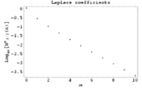
Figure 1: Laplace coefficients for the perturbed potential Eq. (12) for $x=0.5$. Values are plotted on a logarithmic scale ($\log_{10}[b_{1/2}^{m}(x)]$) for $m\in[0..10]$.

3 LINEAR ANALYSIS

How will the disk react to the presence of this quadrupolar or multipolar component in the gravitational field? To answer this question, we can first study its linear response. To do this, we treat each multipolar component as a small perturbation to the equilibrium state prescribed in Sec. 2. The hydrodynamical equations of the accretion disk with adiabatic motion are given by :

$$\frac{\partial\rho}{\partial t}+\mathrm{div}\,(\rho\,\@vec{v}) = 0$$ (14)

$$\frac{\partial\@vec{v}}{\partial t}+(\@vec{v}\cdot\@vec{\nabla}\,)\,\@vec{v} = \@vec{g}-\frac{\@vec{\nabla}\,p}{\rho}$$ (15)

$$\frac{D}{Dt}\left(\frac{p}{\rho^{\gamma}}\right) = 0$$ (16)

All quantities have their usual meanings, $\rho$ being the density of mass in the disk, $\@vec{v}$ the velocity of the disk, $p$ the gaseous pressure, $\gamma$ the adiabatic index and $\@vec{g}$ the gravitational field imposed by the star. Since we are not interested in the accretion process itself, we neglect the viscosity whatever its origin (molecular, turbulent, etc…).

3.1 Lagrangian displacement

Perturbing the equilibrium state with respect to the Lagrangian displacement $\@vec{\xi}$, to first order we get for the Eulerian perturbations of the density, velocity and pressure :

$$\delta\rho = -\,\mathrm{div}\,(\rho\,\@vec{\xi})$$ (17)

$$\delta\@vec{v} = \frac{\partial\@vec{\xi}}{\partial t}+(\@vec{v}\cdot\@vec{\nabla}\,)\,\@vec{\xi}-(\@vec{\xi}\cdot\@vec{\nabla}\,)\,\@vec{v}$$ (18)

$$\delta p = -\,\@vec{\xi}\cdot\@vec{\nabla}\,p-\gamma\,p\,\mathrm{div}\,\@vec{\xi}$$ (19)

Making allowance for a perturbation in the gravitational field and following the Frieman-Rotenberg analysis (Frieman & Rotenberg Frieman1960 (1960)), the Lagrangian displacement satisfies a second order linear partial differential equation :

$$\rho\,\frac{\partial^{2}\@vec{\xi}}{\partial t^{2}}+2\,\rho\,\@vec{v}\cdot\@vec{\nabla}\,\frac{\partial\@vec{\xi}}{\partial t}-\@vec{\nabla}(\gamma\,p\,\mathrm{div}\,\@vec{\xi}+\@vec{\xi}\cdot\@vec{\nabla}\,p)-\mathrm{div}\,(\rho\,\@vec{\xi}\,\@vec{v}\cdot\@vec{\nabla}\,\@vec{v}-\rho\,\@vec{v}\,\@vec{v}\cdot\@vec{\nabla}\,\@vec{\xi})$$

$$+\@vec{g}\,\mathrm{div}\,(\rho\,\@vec{\xi})+\mathrm{div}\,(\rho\,\@vec{\xi})\,\delta\@vec{g} = \rho\,\delta\@vec{g}$$ (20)

We emphasize the fact that the last expression in the above equation contains a term $\mathrm{div}\,(\rho\,\@vec{\xi})\,\delta\@vec{g}$ which is of second order with respect to the perturbation and therefore should be neglected. But in doing so, we suppress the parametric resonance which will be studied in more detail below. Depending on the magnitude of the perturbation, this instability will develop on a timescale closely related to the amplitude of the perturbation and should then not be ignored.

Introducing the convictive derivative by $D/Dt=\partial_{t}+\Omega\,\partial_{\varphi}$, we get for Eq. (3.1) a more concise form :

$$\rho\,\frac{D^{2}\@vec{\xi}}{Dt^{2}}-\@vec{\nabla}(\gamma\,p\,\mathrm{div}\,\@vec{\xi}+\@vec{\xi}\cdot\@vec{\nabla}\,p)-\mathrm{div}\,(\rho\,\@vec{\xi}\,\@vec{v}\cdot\@vec{\nabla}\,\@vec{v})+\@vec{g}\,\mathrm{div}\,(\rho\,\@vec{\xi})+\mathrm{div}\,(\rho\,\@vec{\xi})\,\delta\@vec{g}=\rho\,\delta\@vec{g}$$ (21)

Usually, when evolving in an axisymmetric gravitational field, the above equation reduces to its traditional form where $\delta\@vec{g}=\@vec{0}$. However, in our treatment, due to the gravitational perturbation, a driving force given by $\rho\,\delta\@vec{g}$ appears. Moreover a parametric resonance is also involved due to the term $\mathrm{div}\,(\rho\,\@vec{\xi})\,\delta\@vec{g}$. This will be explained in the next section.

Finding an analytical stability criteria for this system is complicated or even an impossible task. Furthermore, we cannot apply the classical development in plane wave solutions leading to an eigenvalue problem. Indeed, the presence of some coefficients varying periodically in time including $\delta\@vec{g}$ prevent from such a treatment. However, the problem can be cast into a more convenient form if we treat each component of the Lagrangian displacement as independent variables and set the other two components equal to zero. This simplified 3D analysis is done in section 5. But before, we make a complete 2D linear analysis of Eq. (21) in the following section.

4 THIN DISK APPROXIMATION

If we neglect the warping of the accretion disk, we can carry out a more complete 2D linear analysis. Indeed, for a thin accretion disk, its height $H$ is negligible compared to its radius $R$, $(H/R)\approx(c_{\mathrm{s}}/R\,\Omega)\ll 1$. We can give a detailed analysis of the response of the disk to a linear perturbation by setting $\xi_{\mathrm{z}}=0$ in the Eq. (3.1) or Eq. (21).

We seek solutions by writing each perturbation, such as the components of the Lagrangian displacement $\@vec{\xi}$, those of the perturbed velocity $\delta\@vec{v}$, the perturbed density $\delta\rho$, and the perturbed pressure $\delta p$ as

$$X(r,\varphi,t)={\rm Re}[\tilde{X}(r)\,e^{i(m\,\varphi-\sigma\,t)}],$$ (22)

where $m$ is the azimuthal wavenumber and $\sigma$ the eigenfrequency of the perturbation related to the speed pattern $\Omega_{\mathrm{p}}$ by $\sigma=m\,\Omega_{\mathrm{p}}$.

Introducing the new unknown $\psi=\sqrt{r\,p}\,\xi_{\mathrm{r}}$, it can be shown that the problem reduces to the solution of a Schrödinger type equation, (see Appendix A) :

$$\psi^{\prime\prime}(r)+V(r)\,\psi(r)=F(r)$$ (23)

Eq. (23) is the fundamental equation we have to solve to find the solutions to our problem far from the corotation resonance. We refer the reader to Appendix B of (Pétri 2005a , paper I) where we give an analytical method to find approximate solutions to this equation.

The solutions of Eq. (23) divide into two classes of different nature. The first one corresponds to free wave solutions propagating in the accretion disk an associated with the homogeneous part, $F(r)=0$. This gives rise to an eigenvalue problem in which the pattern speed of the perturbation is determined by the specific boundary conditions. The second one consists of a non-wavelike disturbance associated with the inhomogeneous part, $F(r)\neq 0$ due to the gravitational perturbation. Here, the pattern speed of the density perturbation is known and equal to the compact object rotation rate. Therefore, there is no eigenvalue problem at this stage, we need only to solve an usual ordinary differential equation with prescribed initial conditions.

For the purpose of numerical applications, the density profile in the disk has the form $\rho_{0}(r)=\frac{10^{-6}}{r}$. The adiabatic constant is equal to $\gamma=5/3$. The validity of the thin disk approximation in the Newtonian and in the Schwarzschild case is verified by plotting the ratio $H/R$ as shown in Fig. 2. We now discuss them in more details in the next subsections.

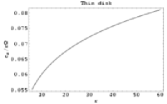
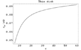
Figure 2: Thin disk approximation in the Newtonian case, on the left and in the Schwarzschild case, on the right. The ratio $H/R=c_{\mathrm{s}}/R\,\Omega$ is plotted and remains less than $1/10$ in the whole disk.

4.1 Free wave solutions

We compute the free wave solutions in order to show the influence of the location of the inner boundary of the disk. When the disk approaches the ISCO, the eigenfrequency of the waves increases. Let’s start with a rough estimate. Looking for free wave solutions, a crude estimate for the radial dependence is given by the WKB expansion as follows :

$$\Psi(r)=\Phi(r)\,e^{i\int^{r}k(s)\,ds}$$ (24)

Putting this approximation into Eq. (23), the dispersion relation is given by :

$$\omega^{2}=\kappa^{2}+c_{\mathrm{s}}^{2}\,k^{2}$$ (25)

Free waves can only propagate in regions where $\omega^{2}-\kappa^{2}=V(r)\,c_{\mathrm{s}}^{2}\geq 0$. The frontier between propagating and damping zone is defined by the inner and outer Lindblad radius $r_{\mathrm{L}}^{in/out}$ defined by $V(r_{\mathrm{L}}^{in/out})=0$. Using the results of Appendix B of paper I, we can guess a better approximation to the solution of the homogeneous Eq. (23) which is valid even for $r\approx r_{\mathrm{L}}^{in/out}$. For the inner Lindblad resonance which is of interest here, we introduce the following function $\omega_{1}$, writing $r_{\mathrm{L}}=r_{\mathrm{L}}^{in}$ :

$$\omega_{1}(r) = -\left[-\frac{3}{2}\,\int_{r_{\mathrm{L}}}^{r}\sqrt{V(s)}\,ds\right]^{2/3}\mathrm{for\;}r\leq r_{\mathrm{L}}$$ (26)

$$\omega_{1}(r) = \left[\frac{3}{2}\,\int_{r_{\mathrm{L}}}^{r}\sqrt{-V(s)}\,ds\right]^{2/3}\mathrm{for\;}r\geq r_{\mathrm{L}}$$ (27)

The function $\psi$ is then a linear combination of the 2 linearly independent solutions :

$$\psi_{1}(r) = \frac{Ai(\omega_{1}(r))}{\sqrt{|\omega_{1}^{\prime}(r)|}}$$ (28)

$$\psi_{2}(r) = \frac{Bi(\omega_{1}(r))}{\sqrt{|\omega_{1}^{\prime}(r)|}}$$ (29)

Furthermore, we impose the solution to remain bounded as one boundary condition, which leads to $C_{2}=0$. Thus the solution for the Lagrangian displacement is : $\xi_{\mathrm{r}}=C_{1}\,\psi_{1}(r)/\sqrt{r\,p}$. At the inner boundary of the accretion disk, the Lagrangian pressure perturbation should vanish. This is expressed as $\Delta p=0$ or equivalently $\mathrm{div}\,\@vec{\xi}=0$. To the lowest order consistent with our approximation, the Lagrangian radial displacement $\xi_{\mathrm{r}}$ must satisfy :

$$\xi^{\prime}(R_{1})+\left(1+2\,m\,\frac{\Omega}{\omega}\right)\,\frac{\xi_{\mathrm{r}}(R_{1})}{R_{1}}=0$$ (30)

This last condition determines the eigenfrequencies $\sigma$ as a function of the azimuthal mode $m$. For any $m$, there is an infinite set of eigenvalues. However, the corresponding eigenfunctions become more and more oscillatory, implying larger and larger wavenumber. In the numerical applications, we shall restrict our attention to the ten first one corresponding also to the highest values $\sigma$.

The eigenvalues for the density waves are shown with decreasing value in Table 1. This holds for a neutron star with angular velocity $\nu_{*}=\Omega_{*}/2\pi=100$ Hz. We compared the Newtonian case with the Schwarzschild metric. The highest speed pattern given by $\sigma/m$ never exceeds the orbital frequency at the ISCO.

Table 1: The ten first highest eigenvalues $\sigma$ for the free wave solutions of Eq. (23). Values are normalized to the frequency of the ISCO, $\Omega_{\mathrm{ISCO}}=6^{-3/2}$. Results are given for 3 azimuthal modes $m=2,5,10$ as well for the Newtonian as for the Schwarzschild gravitational field.

Eigenvalues $\sigma/\Omega_{\mathrm{ISCO}}$
Newtonian			Schwarzschild
$m=2$	$m=5$	$m=10$	$m=2$	$m=5$	$m=10$
0.838519	3.55997	8.22185	1.34337	4.01528	8.62713
0.60303	2.9742	7.26843	0.916075	3.2938	7.56642
0.468333	2.6023	6.6388	0.688728	2.84633	6.87224
0.373567	2.32075	6.15182	0.53807	2.51832	6.34571
0.302154	2.09279	5.74874	0.42896	2.25799	5.91539
0.246424	1.90117	5.40309	0.346084	2.04223	5.5494
0.20198	1.73634	5.09951	0.281241	1.85881	5.22998
0.166046	1.592	4.82837	0.229963	1.69932	4.94587
0.136682	1.46451	4.58301	0.188738	1.55983	4.68884
0.112755	1.35037	4.36067	0.153789	1.43488	4.45707

Some examples of the corresponding eigenfunctions for the density waves are shown in Fig. 3 with arbitrary normalization. Each of them possesses its own inner Lindblad radius depending on the eigenvalue.

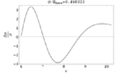
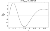
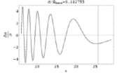
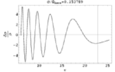
Figure 3: Density wave perturbation in the disk caused by the free wave propagation for the azimuthal mode $m=2$. Some examples are shown for different eigenvalues and for the Newtonian geometry, on the left, as well as for Schwarzschild one, on the right. The vertical bar indicates the location of the inner Lindblad resonance. The normalization of the eigenfunctions is arbitrary.

In a real accretion disk, the precise location of its inner edge does not necessarily reach the ISCO, but can fluctuate due to the varying accretion rate. For instance when the accretion process is enhanced, the inner edge moves closer to the ISCO. As a results the highest eigenvalue of the free waves also increases, see Fig. 4. When the ISCO is reached, the eigenvalues does not change anymore because the boundary conditions remains at the ISCO and the eigenfrequencies saturate. This kind of saturation of the QPO frequency has been observed in some LMXB as reported for instance in a paper by Zhang et al. (Zhang1998 (1998)). The accretion disk has probably reached its ISCO in this particular system. Relating the free wave solutions to this QPO cut off mechanism is not obvious at this stage of our study. Indeed, exciting the waves with a frequency (the star rotation rate $\Omega_{*}$) different from its eigenfrequency ($\sigma$) would require a non-linear process not taken into account in our model so far. However, we will show that already in the linear stage, for sufficiently strong amplitude in the perturbation field, the parametric resonance explains some interesting features of the kHz QPOs (see Sec. 5.2).

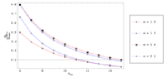
Figure 4: Variation of the highest eigenvalue, corresponding to the eigenfunction having no node, as a function of the location of the inner edge of the disk $R_{\mathrm{in}}$. There is a monotonic increase as the disk approaches the ISCO at $R_{\mathrm{in}}=6\,R_{\mathrm{g}}$. Results are shown for the $m=2,5$ modes in the Newtonian (N) and Schwarzschild (S) spacetime, respectively red and blue curves. The gravitational radius is defined by $R_{\mathrm{g}}=G\,M_{*}/c^{2}$.

4.2 Driven wave perturbations

These driven waves are useful to check our numerical scheme described in Sec. 6. Indeed, in the non-linear simulation, the free wave solutions decay and only the forced solution will survive on a very long timescale. We now solve the full inhomogeneous Eq. (23) to seek for the solution corresponding to the non-wavelike perturbation in the case of a quadrupolar field perturbation. The quadrupolar momentum of the gravitational field due to the non-spherical rotating star is given by :

$$\delta g_{\mathrm{r}}(r,\varphi,t) = \frac{3}{4}\,\frac{G}{r^{4}}\,\left(D_{\mathrm{xx}}+D_{\mathrm{yy}}+(D_{\mathrm{xx}}-D_{\mathrm{yy}})\,e^{2\,i\,(\varphi-\Omega_{*}\,t)}\right)$$ (31)

$$\delta g_{\varphi}(r,\varphi,t) = \frac{i}{2}\,\frac{G}{r^{4}}\,(D_{\mathrm{xx}}-D_{\mathrm{yy}})\,e^{2\,i\,(\varphi-\Omega_{*}\,t)}$$ (32)

In the numerical applications, we choose $D_{\mathrm{xx}}$ and $D_{\mathrm{yy}}$ such that $D_{\mathrm{xx}}+D_{\mathrm{yy}}$ remains negligible with respect to $D_{\mathrm{xx}}-D_{\mathrm{yy}}$. In the complex amplitudes of $\delta g_{\mathrm{r/\varphi}}$ we therefore only keep the radial dependence for the mode $m=2$. Thus :

$$\delta g_{\mathrm{r}}(r) = \frac{3}{4}\,\frac{G}{r^{4}}\,(D_{\mathrm{xx}}-D_{\mathrm{yy}})$$ (33)

$$\delta g_{\varphi}(r) = \frac{i}{2}\,\frac{G}{r^{4}}\,(D_{\mathrm{xx}}-D_{\mathrm{yy}})$$ (34)

We have to solve the second order ordinary differential equation for $\psi$ with the appropriate boundary conditions Eq. (30). The solution is :

$$\psi_{\mathrm{r}}(r)=C_{1}\,\psi_{1}(r)+C_{2}\,\psi_{2}(r)+\pi\,\mathrm{sign}(\omega_{1}^{\prime}(r))\,\int_{r_{\mathrm{L}}}^{r}\left(\psi_{1}(r)\,\psi_{2}(s)-\psi_{1}(s)\,\psi_{2}(r)\right)F(s)\,ds$$ (35)

The constant $C_{2}$ is chosen such that the solution remains bounded for $r\gg r_{\mathrm{L}}$ :

$$C_{2}=\lim_{r\to\infty}\pi\,\mathrm{sign}(\omega_{1}^{\prime})\,\int_{r_{\mathrm{L}}}^{r}\psi_{1}(s)\,F(s)\,ds$$ (36)

This integral is convergent because the function $\psi_{1}$ is exponentially decreasing with the radius.

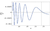
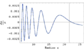
Figure 5: Non-wavelike density perturbation in a Newtonian potential, on the left, and in a Schwarzschild potential, on the right, for the mode $m=2$ and the speed pattern $\sigma=2\,\Omega_{*}$. The amplitude of the disturbances is related to the strength of the gravitational perturbation and is therefore not arbitrary.

The analytical solutions Eq. (35) agree well with the direct numerical integration of Eq. (23). On the Fig. 5, there is no graphical distinction between them nor for the Newtonian potential neither for the Schwarzschild field.

4.3 Corotation resonance

The corotation resonance is defined by the radius $r_{\mathrm{c}}$ where $\omega_{*}(r_{\mathrm{c}})=0$. Actually, this equation possesses two solutions corresponding to $\omega(r_{\mathrm{c}})=\pm\frac{m\,c_{\mathrm{s}}(r_{\mathrm{c}})}{r_{\mathrm{c}}}$. The width of this region is of the order of the disk height $O(H)$. For very thin disks, this discrepancy can be neglected and the two solutions merge together in an unique corotation radius given by $\omega(r_{\mathrm{c}})=0$. In other words, we assume in this case that $\omega=\omega_{*}$. However, in our numerical application, the separation between the two corotation radii is large enough to be resolved. For the detailed study of both corotation, we have to use the more accurate Eq. (A). Keeping only the leading divergent terms in the coefficients of the ordinary differential equation, we obtain :

$$\frac{m^{2}\,c_{\mathrm{s}}^{4}}{r^{2}\,\omega_{*}^{2}}\,\xi_{\mathrm{r}}^{\prime\prime}(r)+\frac{m^{2}\,c_{\mathrm{s}}^{4}}{r^{2}}\,\frac{d}{dr}\left(\frac{1}{\omega_{*}^{2}}\right)\,\xi_{\mathrm{r}}^{\prime}(r)+2\,\frac{m\,c_{\mathrm{s}}^{2}\,\Omega\,\omega}{r}\,\frac{d}{dr}\left(\frac{1}{\omega_{*}^{2}}\right)\,\xi_{\mathrm{r}}(r)=i\frac{m\,c_{\mathrm{s}}^{2}}{r}\,\frac{d}{dr}\left(\frac{1}{\omega_{*}^{2}}\right)\,\delta g_{\varphi}(r)$$

We introduce the new independent variable :

$$x=\frac{r-r_{\mathrm{c}}}{r_{\mathrm{c}}}$$ (38)

Developing $\omega_{*}$ to the first order around the corotation radius $r_{\mathrm{c}}$ we have :

$$\omega_{*}(r)=\omega_{*}(r_{\mathrm{c}})+(r-r_{\mathrm{c}})\,\omega_{*}^{\prime}(r_{\mathrm{c}})+o(r-r_{\mathrm{c}})=x\,r_{\mathrm{c}}\,\omega_{*}^{\prime}(r_{\mathrm{c}})+o(x)\approx\alpha\,x$$ (39)

To this approximation, we have to solve :

$$\xi_{\mathrm{r}}^{\prime\prime}(x)-\frac{2}{x}\,\xi_{\mathrm{r}}^{\prime}(x)-4\,\frac{\Omega\,\omega\,r_{\mathrm{c}}^{2}}{m\,c_{\mathrm{s}}^{2}\,x}\,\xi_{\mathrm{r}}(x)=-2\,i\,\frac{r_{\mathrm{c}}^{2}\,\delta g_{\varphi}(r_{\mathrm{c}})}{m\,c_{\mathrm{s}}^{2}\,x}$$ (40)

This is of the form :

$$y^{\prime\prime}(x)-\frac{2}{x}\,y^{\prime}(x)-\frac{b}{x}\,y(x)=\frac{c}{x}$$ (41)

with $b=4\,\frac{\Omega\,\omega\,r_{\mathrm{c}}^{2}}{m\,c_{\mathrm{s}}^{2}\,x}\geq 0$ and $c=-2\,i\,\frac{r_{\mathrm{c}}^{2}\,\delta g_{\varphi}(r_{\mathrm{c}})}{m\,c_{\mathrm{s}}^{2}}$. Making the change of variable $t=2\,\sqrt{b\,x}$ and introducing the new unknown $v(t)$ by $y(t)=t^{3}\,v(t)$, it can be shown that $v(t)$ satisfies the modified Bessel equation of order 3 :

$$v^{\prime\prime}(t)+\frac{1}{t}\,v^{\prime}(t)-(1+\frac{9}{t^{2}})\,v(t)=0$$ (42)

This is solved by :

$$v(t)=C_{1}\,I_{3}(t)+C_{2}\,K_{3}(t)$$ (43)

Thus, the complete most general solution to Eq. (40) for which a particular solution is easily found to be a constant equal to $\xi_{\mathrm{r}}^{p}(r)=i\,\frac{\delta g_{\varphi}(r_{\mathrm{c}})}{2\,\Omega\,\omega}$, is

$$\xi_{\mathrm{r}}(x)=C_{1}\,x^{3/2}\,I_{3}(2\,\sqrt{b\,x})+C_{2}\,x^{3/2}\,K_{3}(2\,\sqrt{b\,x})+i\,\frac{\delta g_{\varphi}(r_{\mathrm{c}})}{2\,\Omega\,\omega}$$ (44)

Finally, near the corotation radius, the Lagrangian displacement which remains bounded needs $C_{1}=0$ :

$$\xi_{\mathrm{r}}(x)=C_{2}\,x^{3/2}\,K_{3}(2\,\sqrt{b\,x})+i\,\frac{\delta g_{\varphi}(r_{\mathrm{c}})}{2\,\Omega\,\omega}$$ (45)

The density disturbance induced in the disk by the rotating gravitational perturbation is then to the lowest order :

$$\frac{\delta\rho}{\rho}=-\frac{\mathrm{div}\,(\rho\@vec{\xi})}{\rho}=-\frac{1}{\rho\,r}\,\frac{d}{dr}(r\,\rho\,\xi_{\mathrm{r}})+i\,\frac{m}{r\,\omega_{*}^{2}}\,\left(\delta g_{\varphi}+2\,i\,\Omega\,\omega\,\xi_{\mathrm{r}}\right)$$ (46)

The displacement Eq. (45) is continuous and differentiable everywhere. Thus, the first term on the right hand side has a finite value. The second term on the RHS needs a special treatment. Indeed, when $r$ approaches $r_{\mathrm{c}}$ the numerator and the denominator vanish as well, leaving us with an undetermined expression of the form $0/0$. To find the behavior near $r_{\mathrm{c}}$ we note that near the corotation, $(\delta g_{\varphi}+2\,i\,\Omega\,\omega\,\xi_{\mathrm{r}})$ behaves as $(\delta g_{\varphi}(r)-\delta g_{\varphi}(r_{\mathrm{c}}))=\delta g_{\varphi}^{\prime}(r_{\mathrm{c}})\,(r-r_{\mathrm{c}})$ with $\delta g_{\varphi}^{\prime}(r_{\mathrm{c}})\neq 0$. Thus we conclude that it approaches zero as $x$ and

$$\frac{\delta\rho}{\rho}\approx i\,\frac{m\,\delta g_{\varphi}^{\prime}(r_{\mathrm{c}})}{\omega_{*}^{\prime}(r_{\mathrm{c}})^{2}\,r_{\mathrm{c}}^{2}\,x}$$ (47)

The divergent term in the density perturbation Eq. (47) tends to infinity as $\frac{1}{x}$. This result is consistent with the conclusions drawn by Goldreich & Tremaine (Goldreich1979 (1979)) for a disk without self-gravity.

From the comparison between Newtonian and Schwarzschild geometry, we conclude that the introduction of general relativistic effects as the ISCO does not changes the qualitative behavior of the disk response. The ISCO only shifts the location of the Lindblad resonances and the eigenvalues of the free wave solutions.

4.4 Counterrotating disk

We can also use the previous analysis for a counterrotating accretion disk. Because the spin of the star does not intervene in the homogeneous Schrödinger equation, the free wave solutions remain identical to the above mentioned results. The only change comes from the non-wavelike disturbance for which we have to replace $\Omega_{*}\rightarrow-\Omega_{*}$. Following the same outline as in 4.2, we solve numerically the inhomogeneous Schrödinger equation and we also looked for an analytical approximate solution. The results showing the density perturbation is plotted in Fig. 6. The two solutions are graphically indistinguishable, the discrepancy is less than 1 %. In this special case, the Lindblad resonances do not appear anymore in the computational domain.

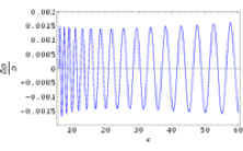
Figure 6: Density perturbation $\delta\rho/\rho$ in the counterrotating disk evolving in a Newtonian potential. Results are given for the mode $m=2$ and the eigenvalue $\sigma=-2\,\Omega_{*}$.

5 SIMPLIFIED ANALYSIS

5.1 The eigenvalue problem

To get more insight in the nature of the resonances, we focus now only on the displacement of the disk in each direction independently, setting $\xi_{i}=0$ in the other directions. This means that we neglect the coupling between the oscillations occurring in perpendicular directions. Despite this simplification, this will help us to bring out the meaning of the oscillations and to derive some resonance conditions without removing any physically meaningful mechanism.

Let’s begin the study with the motion in the vertical direction, setting $(\xi_{\mathrm{r}},\xi_{\varphi})=0$, we find :

$$\rho\,\frac{D^{2}\xi_{\mathrm{z}}}{Dt^{2}}-\frac{\partial}{\partial z}\left(\gamma\,p\,\frac{\partial\xi_{\mathrm{z}}}{\partial z}\right)-\rho\,\xi_{\mathrm{z}}\,\frac{\partial g_{\mathrm{z}}}{\partial z}+\frac{\partial}{\partial z}\left(\rho\,\xi_{\mathrm{z}}\right)\,\delta g_{\mathrm{z}}=\rho\,\delta g_{\mathrm{z}}$$ (48)

Developing the vertical component of the gravity near the equatorial plane to the first order in $z$, it can be cast into the form $g_{\mathrm{z}}(r,z)=-\kappa_{\mathrm{z}}^{2}(r)\,z$. The vertical epicyclic frequency $\kappa_{\mathrm{z}}$ depends only on the radius. So we get :

$$\frac{D^{2}\xi_{\mathrm{z}}}{Dt^{2}}-\frac{1}{\rho}\,\frac{\partial}{\partial z}\left(\rho\,c_{\mathrm{s}}^{2}\,\frac{\partial\xi_{\mathrm{z}}}{\partial z}\right)+\kappa_{\mathrm{z}}^{2}\,\xi_{\mathrm{z}}+\frac{1}{\rho}\,\frac{\partial}{\partial z}\left(\rho\,\xi_{\mathrm{z}}\right)\,\delta g_{\mathrm{z}}=\delta g_{\mathrm{z}}$$ (49)

We have introduced the sound speed by $c_{\mathrm{s}}^{2}=\frac{\gamma\,p}{\rho}$.

The same can be done for the radial motion by setting $(\xi_{\mathrm{z}},\xi_{\varphi})=0$, we obtain a similar expression :

$$\frac{D^{2}\xi_{\mathrm{r}}}{Dt^{2}}-\frac{1}{\rho\,r}\,\frac{\partial}{\partial r}\left(\rho\,c_{\mathrm{s}}^{2}\,r\,\frac{\partial\xi_{\mathrm{r}}}{\partial r}\right)+\kappa_{\mathrm{r}}^{2}\,\xi_{\mathrm{r}}+\frac{1}{\rho\,r}\,\frac{\partial}{\partial r}\left(r\,\rho\,\xi_{\mathrm{r}}\right)\,\delta g_{\mathrm{r}}=\delta g_{\mathrm{r}}$$ (50)

The exact value of the radial epicyclic frequency depends on the pressure distribution in the disk.

Eq. (49) and (50) look very similar, the discrepancy coming only from the difference between the planar and the cylindrical geometry (terms containing $r$). We recognize in the two first terms of Eq. (49) and (50) a sound wave propagation equation in a tube of spatial varying but time independent cross section (Morse & Feshbach Morse1953 (1953)). The first and third term put together is an harmonic oscillator at the epicyclic frequency $\kappa_{\mathrm{r/z}}$. So the three first terms are a generalization of the Klein-Gordon equation and do not give rise to any kind of instability. The interesting part are those containing the perturbation in the gravitational field $\delta g_{\mathrm{r/z}}$. Neglecting the sound wave propagation, we recognize a kind of Hill equation corresponding to an oscillator with periodically time-varying eigenfrequency. It is well known that this type of equation shows what is called a parametric resonance. Moreover due to the rotation of the star, this perturbation will vary sinusoidally in time and the Hill equation specializes to the Mathieu equation for which we know the resonance conditions. Indeed, Mathieu equation written in the form

$$y^{\prime\prime}(t)+\omega_{0}^{2}\,(1+h\,\cos\gamma\,t)\,y(t)=0$$ (51)

becomes unstable if the excitation frequency $\gamma=2\frac{\omega_{0}}{n}$ where $n$ is an integer (Landau & Lifshitz Landau1982 (1982)). Note that the resonant frequency does not depend on the amplitude $h$. The corresponding growth rates are proportional to $h^{n}$. For small amplitudes of the excitation term, only the first few integer $n$, let’s say $n\leq 5$, are relevant for this parametric instability.

The equation contains also an harmonic oscillator excited by a driven force given by $\delta g_{\mathrm{r/z}}$. This gives rise to the well known driven resonance.

A careful analysis of Eq. (49) and Eq. (50) shows that in the frame locally corotating with the disk, the Lagrangian displacement feels a modulation due to the gravity perturbation term $\delta g_{\mathrm{r/z}}$. In this corotating frame, its time dependence contains expressions like $\cos m(\varphi-(\Omega_{*}-\Omega)\,t)$ and $\sin m(\varphi-(\Omega_{*}-\Omega)\,t)$, (Eq. 2.2). Therefore the modulation occurs at a frequency $m\,|\Omega_{*}-\Omega|$. Each Fourier mode of the perturbed gravitational field contributes to give its proper modulation frequency.

From this analysis we expect three kind of resonances corresponding to :

• a corotation resonance at the radius where the angular velocity of the disk equals the rotation speed of the star. This is only possible for prograde disks. The resonance condition to determine the corotating radius is simply :

  $$\Omega=\Omega_{*}$$ (52)

• a inner and outer Lindblad resonances at the radius where the radial or vertical epicyclic frequency equals the frequency of each mode of the gravitational potential as seen in the locally corotating frame. We find the resonance condition to be :

  $$m\,|\Omega_{*}-\Omega|=\kappa_{\mathrm{r/z}}$$ (53)

  The name for this resonance arises from the analogy with the theory of density waves met in the context of the spiral structure in galactic dynamics. If the pressure acts as a restoring force in the vertical direction, the derivation of the vertically driven resonances is given by $m\,|\Omega_{*}-\Omega|=\sqrt{1+\Gamma}\,\kappa_{\mathrm{z}}$, where $\Gamma=\partial\ln P/\partial\ln\rho$ is the effective adiabatic index, (see Lubow Lubow1981 (1981)). We will not go into such refinement for a first approach to the resonance problem.

• a parametric resonance related to the time-varying epicyclic frequency, (Hill equation). The rotation of the star induces a sinusoidally variation of the epicyclic frequency leading to the well known Mathieu’s equation. The resonance condition can be derived as followed :

  $$m\,|\Omega_{*}-\Omega|=2\,\frac{\kappa_{\mathrm{r/z}}}{n}$$ (54)

Note that the driven resonance is a special case of the parametric resonance for $n=2$. However, their growth rate differ by the timescale of the amplitude magnification. Driving causes a linear growth in time while parametric resonance causes an exponential growth.

The parametric resonance condition Eq. (54) has been derived on the basis of a single particle orbit perturbation without taking into account the fluid description of the gas. Hirose and Osaki (Hirose1990 (1990)) applied this method in the context of tidally distorted accretion disk in cataclysmic variable. However, Lubow (Lubow1991 (1991)) showed that a more careful treatment of the resonances in the hydrodynamical case leads to some eccentric instability as well to unstable tilt of the accretion disk due to mode coupling (Lubow Lubow1992 (1992)). Due to the effect introduce by the fact that the disk is a fluid, the growth rate of this instability is only quadratic in the strength of the tidal force. Nevertheless, another parametric instability arising in a tidally distorted accretion disk has been introduced by Goodman (Goodman1993 (1993)). He showed that the growth rate is linear in the tidal force amplitude and propagates only in a three-dimensional disk.

5.2 Results

5.2.1 Newtonian disk

From the resonance conditions derived above, Eq. (53) and Eq. (54), we can find the radii where each of this resonance will occur. Beginning with the Newtonian potential, it is well known that the angular velocity, the radial and epicyclic frequencies for a single particle are all equal so that $\Omega=\kappa_{\mathrm{r}}=\kappa_{\mathrm{z}}$. This conclusion remains true for a thin accretion disk having $c_{\mathrm{s}}/R\,\Omega\ll 1$. Distinguishing between the two signs of the absolute value, we get for the parametric resonance condition Eq. (54), which includes the Lindblad resonance for the special case $n=2$, the following orbital rotation rate :

$$\frac{\Omega}{\Omega_{*}}=\frac{m}{m\pm 2/n}$$ (55)

As a consequence, the resonances are all located in the frequency range $\Omega\in[\Omega_{*}/3,3\,\Omega_{*}]$.

In table 2, we indicate the results for a $300$ Hz and a $600$ Hz spinning neutron star and for the first three mode $m$ and for the integer $n=1,2$. Because of the degeneracy $\kappa_{\mathrm{r}}=\kappa_{\mathrm{z}}$, the resonances in the radial and vertical directions occur at exactly the same locations.

Table 2: Value of the orbital frequencies at the parametric resonance radii for the first three order $n$ in the case of a Newtonian gravitational potential. The results are given for a $1.4\,\mathrm{M}_{\odot}$ neutron star rotating respectively at $300$ Hz and $600$ Hz. The value on the left of the symbol / corresponds to the absolute value sign taken to be - and on the right to be +.

Azimuthal mode $m$	Orbital frequency $\nu(r,a)$ (Hz)
	$\nu_{*}=600$ Hz		$\nu_{*}=300$ Hz
	$n=1$	$n=2$	$n=1$	$n=2$
1	-600 / 200	—- / 300	-300 / 100	— / 150
2	—- / 300	1200 / 400	— / 150	600 / 200
3	1800 / 360	900 / 450	900 / 180	450 / 225

The pair of highest orbital frequencies for the $\nu_{*}=300$ Hz spinning neutron star are $\nu_{1}=900$ Hz and $\nu_{2}=600$ Hz. The peak separation frequency is then $\Delta\nu=300$ Hz $=\nu_{*}$. The vertical motion induced by the parametric resonance at that location will appear as a modulation in the luminosity of the accretion disk. For the 600 Hz spinning neutron star, the highest orbital frequencies are 1800 Hz and 1200 Hz. However, due to the ISCO, the former one is not observed because it is located inside the ISCO and therefore does not correspond to a stable orbit. Therefore, the first two highest observable frequencies are $\nu_{1}=1200$ Hz and $\nu_{2}=900$ Hz. The peak separation frequency becomes then $\Delta\nu=300$ Hz $=\nu_{*}/2$. Thus the peak separation for slow spinning neutron stars is $\Delta\nu=\nu_{*}$ whereas for fast spinning neutron star the peak separation is $\Delta\nu=\nu_{*}/2$. This segregation between slow and fast rotating neutron stars is well observed in several accreting systems (van der Klis vanderKlis2004 (2004)). These conclusions confirm the results already obtained in the single particle approximation (Pétri 2005b , 2005c ).

We believe that only oscillations in the vertical direction can give rise to significant periodic changes in the accretion disk luminosity. However, resonances associated with the radial epicyclic frequency are shown because we start with a 2D study in the equatorial plane (linear analysis and numerical simulations). Radial oscillations in the disk are hardly observable because they will not lead to a significant change in the luminosity as would be the case for a warped disk for instance. The warping is induced at some preferred radii where the resonance conditions for vertical oscillations are fulfilled. This study would necessitate a full 3D treatment of the accretion disk which is left for future work. Nevertheless, the properties of the propagation of waves in a three-dimensional accretion disk have been investigated by many authors. Lubow and Pringle (Lubow1993 (1993)) studied the linear behavior of free waves in an isothermal disk. Korycansky and Pringle (Korycansky1995 (1995)) extended this work to the case of polytropic disks and showed that the local 2D dispersion relation is not valid anymore. Due to the stratified vertical structure, waves are refracted and reach the surfaces of the disk (Lin et al. 1990a ). This happens within a distance of the order of $r_{\mathrm{L}}/m$ and is called wave-channeling by Lubow & Ogilvie (Lubow1998 (1998)) who undertook a detailed study of the wave propagation in the neighborhood of the Lindblad resonances. Finally, the 3D response to a tidal force was explored by Lin et al. (1990b ). The behaviour of the waves launched at the resonance radii (corotation, Lindblad and parametric) propagating in the 3D disk is a complicated task. In this paper, we just start with a simple picture, focusing on the resonances itself without taking into account the propagation of the disturbances.

5.2.2 General relativistic disk

When the inner edge of the accretion disk reaches values of a few gravitational radii, the general relativistic effects become important. The degeneracy between the three frequencies $\Omega$, $\kappa_{\mathrm{r}}$ and $\kappa_{\mathrm{z}}$ will be removed and they will depend on the angular momentum of the star $a$. Indeed we distinguish 3 characteristic frequencies in the accretion disk around a Kerr black hole (or a rotating neutron star) :

• the orbital angular velocity :

  $$\Omega(r,a)=\frac{1}{r^{3/2}+a}$$ (56)

• the radial epicyclic frequency :

  $$\kappa_{\mathrm{r}}(r,a)=\Omega(r,a)\,\sqrt{1-\frac{6}{r}+8\,\frac{a}{r^{3/2}}-3\,\frac{a^{2}}{r^{2}}}$$ (57)

• the vertical epicyclic frequency :

  $$\kappa_{\mathrm{z}}(r,a)=\Omega(r,a)\,\sqrt{1-4\,\frac{a}{r^{3/2}}+3\,\frac{a^{2}}{r^{2}}}$$ (58)

The parameter $a$ corresponds to the angular momentum of the star, in geometrized units. We also assume that $G\,M_{*}=1$. For a neutron star of mass $M_{*}$ and rotating at the angular velocity $\Omega_{*}$, it is given by $a=\frac{c\,I_{*}}{G\,M_{*}^{2}}\,\Omega_{*}$.

We have the following ordering :

$$\Omega>\kappa_{\mathrm{z}}>\kappa_{\mathrm{r}} for \;\;a>0$$ (59)

$$\kappa_{\mathrm{z}}>\Omega>\kappa_{\mathrm{r}} for \;\;a<0$$ (60)

The parametric resonance conditions Eq. (54) splitted into the two cases become :

$$\Omega(r,a)\pm\frac{2\,\kappa_{\mathrm{r/z}}(r,a)}{m\,n}=\Omega_{*}$$ (61)

For a given angular momentum $a$, we have to solve these equations for the radius $r$. For a neutron star, we adopt the typical parameters :

• mass $M_{*}=1.4\,\mathrm{M}_{\odot}$ ;

• angular velocity $\nu_{*}=\Omega_{*}/2\pi=300-600$ Hz ;

• moment of inertia $I_{*}=10^{38}\;kg\,m^{2}$ ;

• angular momentum $a_{*}=\frac{c\,I_{*}}{G\,M_{*}^{2}}\,\Omega_{*}$.

The angular momentum is then given by $a_{*}=5.79*10^{-5}\,\Omega_{*}$. Solving Eq. (61) for the radius and then deducing the orbital frequency at this radius we get the results shown in tables 3 and 4. For the spin rate of the star we find $a_{*}=0.1-0.2$ and so the vertical epicyclic frequency remains close to the orbital one $\kappa_{\mathrm{z}}\approx\Omega$. Thus for the vertical resonance, we are still approximately in the Newtonian case mentioned in the previous section and the same conclusions apply here to. Consequently, the relativistic results are the same as those discussed in the previous section dealing with a Newtonian disk. The only difference comes from the presence of the ISCO added in a self-consistent way by changing the behaviour of the radial epicyclic frequency which vanishes at the inner edge.

Table 3: Value of the orbital frequencies at the radial parametric resonance radii for the first three order $n$ in the general relativistic Kerr spacetime. The results are given for a $1.4\,\mathrm{M}_{\odot}$ neutron star rotating respectively at $300$ Hz and $600$ Hz. The value on the left of the symbol / corresponds to the absolute value sign taken to be - and on the right to be +.

Azimuthal mode $m$	Orbital frequency $\nu(r,a)$ (Hz)
	$\nu_{*}=600$ Hz		$\nu_{*}=300$ Hz
	$n=1$	$n=2$	$n=1$	$n=2$
1	2542 / 212	1566 / 319	1257 / 106	779 / 159
2	1566 / 318	955 / 419	779 / 159	477 / 210
3	1135 / 380	809 / 468	566 / 190	404 / 234

Table 4: Value of the orbital frequencies at the vertical parametric resonance radii for the first three order $n$ in the general relativistic Kerr spacetime. The results are given for a $1.4\,\mathrm{M}_{\odot}$ neutron star rotating respectively at $300$ and $600$ Hz. The value on the left of the symbol / corresponds to the absolute value sign taken to be - and on the right to be +.

Azimuthal mode $m$	Orbital frequency $\nu(r,a)$ (Hz)
	$\nu_{*}=600$ Hz		$\nu_{*}=300$ Hz
	$n=1$	$n=2$	$n=1$	$n=2$
1	—- / 200	—- / 300	— / 100	— / 150
2	—- / 300	1198 / 400	— / 150	599 / 200
3	1790 / 360	899 / 450	898 / 180	450 / 225

We emphasize the fact that these results apply to a rotating asymmetric magnetic field with exactly the same resonance conditions Eq. (52)-(53)-(54) provided that the flow is not to far from its Keplerian motion, i. e. a weakly magnetized accretion disk with high $\beta$-plasma parameter where this parameter is defined by (Delcroix & Bers Delcroix1994 (1994), see also paper I) :

$$\beta=\frac{p}{B^{2}/2\mu_{0}}$$ (62)

$p$ being the pressure and $B$ the local magnetic field strength.

6 NUMERICAL SIMULATIONS

Now we have identified the resonance location (Lindblad, parametric and corotation) in the disk due to the perturbation in the gravitational field, we go further to include the full non linearities of the hydrodynamical equations by performing 2D simulations in the ($r,\varphi$) plane. This is the goal of the next section.

6.1 Linear analysis

In order to check the numerical pseudo-spectral code, we solve the full non-linear HD equations with a weak $m=2$ azimuthal perturbation. We retrieve the results mentioned in section 4.2. This is discussed in the following subsections.

We use the geometrized units for which $G=c=1$. The distances are measured with respect to the gravitational radius given by $R_{\mathrm{g}}=G\,M_{*}/c^{2}$. Moreover, the simulations are performed for a star with $M_{*}=1$ so that in the new units we have $R_{\mathrm{g}}=1$. In all the simulations presented below, the star is assumed to be an ellipsoid with the main axis given by $R_{\mathrm{x}}=R_{\mathrm{z}}\neq R_{\mathrm{y}}$. The standard resolution is $N_{\mathrm{R}}\times N_{\varphi}=256\times 32$ where $N_{\mathrm{R}}$ and $N_{\varphi}$ are the number of grid points in the radial and azimuthal direction respectively.

Before the time $t=0$, the disk stays in its axisymmetric equilibrium state and possesses only an azimuthal motion. At $t=0$, we switch on the perturbation by adding the quadrupolar component to the gravitational field. We then let the system evolve during more than one thousand orbital revolutions of the inner edge of the disk. We performed four sets of simulations. In the first one, the gravitational potential was Newtonian. In the second one, we used a pseudo-Newtonian potential in order to take into account the ISCO. This is well suited to describe the Schwarzschild spacetime. In the third one, we took into account the angular momentum of the star by introducing a pseudo-Kerr geometry. And finally in the fourth and last set, we performed simulations with a counter rotating accretion disk evolving in a Newtonian potential described in the first set.

We perform the simulation in the thin disk limit. For this thin gaseous disk, there is a slightly difference of the order $(H/R)^{2}$ between the single particle characteristic frequencies and the true disk frequencies where $H$ is the typical height of the disk and $R$ its radius. Indeed, inspecting Eq. (50) and neglecting the gravitational perturbation $\delta g_{\mathrm{r}}$, a rough estimation in order of magnitude gives $\partial/\partial r\approx R^{-1}$ and due to the thin disk approximation we also have $c_{\mathrm{s}}\approx\Omega_{\mathrm{k}}\,H$ where $\Omega_{\mathrm{k}}$ is the Keplerian orbital frequency for a single particle. Therefore the coefficient in front of $\xi_{\mathrm{r}}$ is approximately $\Omega_{\mathrm{k}}^{2}\,(1-H^{2}/R^{2}$), baring in mind that $\kappa_{\mathrm{r}}\approx\Omega_{\mathrm{k}}$ and proving the aforementioned statement. In all our simulations, we choose the physical parameters such that this ratio remains less than $1/10$, spanning roughly from $0.05$ to $0.09$. In such a way the single particle approximation remains valid within 10 %. Typical behaviors of the ratio $H/R$ are depicted for the Newtonian and Schwarzschild case in Fig. 2. If the disk were assumed to be thick so that $H\approx R$, the difference between single particle and fluid frequency can be appreciable. Moreover, the orbital motion remains no longer Keplerian in such a geometry. We now deal with the results.

6.2 Newtonian potential

First, we study the behavior of the thin disk in the Newtonian potential. In this case, the Keplerian rotation rate, the vertical and the radial epicyclic frequencies for a single particle are all identical as discussed before. To a good approximation we have :

$$\Omega_{\mathrm{k}}\approx\kappa_{\mathrm{r}}\approx\kappa_{\mathrm{z}}$$ (63)

The star normalized rotation rate around the z-axis is equal to $\Omega_{*}=0.0043311$. Assuming a $1.4\,\mathrm{M}_{\odot}$ neutron star, this corresponds to a spin of $\nu_{*}=100.0$ Hz. The disk inner boundary is located at $R_{1}=6.0$ while the outer boundary is located at $R_{2}=60.0$. The orbital angular motion at the inner edge of the disk is $\Omega_{\mathrm{in}}=R_{1}^{-3/2}=0.0680$. We normalize the time by dividing it by the spin period of the star $T_{*}=\frac{2\,\pi}{\Omega_{*}}=1450.7$.

The time evolution of the density perturbation in the disk calculated as $\Delta\rho/\rho_{0}=\rho/\rho_{0}-1$ is shown in Fig. 7. The corotation resonance located at $r=40.0$ expected from the condition Eq. (52) is not visible at this stage. Indeed the weak linear growth rate makes the corotation resonance relevant only after a few $10^{5}$ orbital revolutions which is hundreds of time more than the time of the simulation. However, after a few hundred of orbital revolutions, the disk settles down to a new quasi-stationary state in which the inner and outer Lindblad resonances persist. This happens after a transition regime where density waves leave the disk by crossing its edges. Almost all of the energy put into the disk by the star’s rotation leaves the computational domain at its inner and outer edges. The non reflecting boundary conditions act as a kind of viscosity strongly damping the oscillations. We refer the reader to paper I for the method of implementation of these non reflecting boundary conditions. This is confirmed by inspection of the Fig. 8 in which we have plotted a cross section of the final density perturbation $\delta\rho/\rho_{0}$ for a given azimuthal angle, namely $\varphi=0$. As expected the density perturbation vanishes at the disk edges. The shape of this perturbation agrees well with the linear analysis. Indeed comparing Fig. 8 and the left part of Fig. 5, the only small difference comes from the different boundary conditions imposed. Nevertheless, the location of the inner and outer Lindblad resonances as well as the number of roots of each function and the maximum amplitude are equal.

The nonlinearities are therefore weak for the whole simulation duration. Indeed, looking at the Fourier spectrum of the density in Fig. 9, where the amplitude of each component is plotted vs the mode $m$ on a logarithmic scale. The odd modes are not present. However, the weak nonlinearities create a cascade to high even modes starting with $m=2$. The largest asymmetric expansion coefficient $C_{m}$ is $m=2$, the next even coefficients follow roughly a geometric series with a factor $q=10^{-3}$, so we can write for all $m$ even, $C_{m}\approx q^{m/2-1}\,C_{2}$ until they reach values less than $10^{-20}$ which can be interpreted as zero from a numerical point of view. The deviation from the stationary state being weak, the amplitudes of these even modes decay compared to the previous one, the highest being of course $m=2$. Thus, even in the full non linear simulation, the regime remains quasi linear. As a conclusion, the parametric resonance phenomenon discussed in the previous section is irrelevant at this stage of our work. The effect of strong nonlinearity putting the system out of its linear regime will be studied in a forthcoming paper. Note that due to the desaliasing process, the modes $m\geq 9$ are all set to zero. Note also that the free wave solutions leave the computational domain and are no longer present. Only the non-wavelike disturbance produces significant changes in the density profile.

The resolution of $256\times 32$ which seems rather low is nevertheless justified by the fact that the components of the Fourier-Tchebyshev transform decay rapidly and become negligible after the first few terms in the Fourier expansion and after the first 30 or 40 terms in the Tchebyshev expansion. In order to check that this resolution is however sufficient, we performed a new set simulation by increasing the number of grid points by a factor two in both coordinates, namely we used a resolution of $512\times 64$. The density perturbation is then given by the Fig. 10 and the Fourier expansion coefficients in Fig. 11 which have to be compared respectively with Fig. 7 and Fig. 9. The desaliasing process does not affect the Fourier coefficient because they vanish already well before $m=19$. This proves that the structure is spatially fully resolved with both resolutions. Indeed, there is actually no significant difference between the 2 pictures. The lowest resolution reaches already a very good numerical precision. We therefore keep this $256\times 32$ resolution in the next sections.

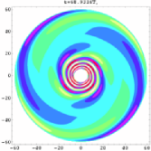
Figure 7: Final snapshot of the density perturbation $\delta\rho/\rho_{0}$ in the accretion disk evolving in a quadrupolar perturbed Newtonian potential. The disk extends from $R_{1}=6.0$ to $R_{2}=60.0$. The rotation rate of the star is $\Omega_{*}=0.0043311$. The time is normalized to the spin period $T_{*}=1450.7$. The $m=2$ structure emerges in relation with the $m=2$ quadrupolar potential perturbation.

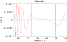
Figure 8: Cross section of the density perturbation $\delta\rho/\rho_{0}$ in the Newtonian disk at the final time of the simulation. The inner and outer Lindblad resonances appear clearly at $r_{\mathrm{L}}^{in/out}=23.7/49.3$. When crossing the corotation resonance the density curve shows a break in its slope.

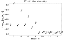
Figure 9: Amplitude of the Fourier components of the density perturbation. $t_{f}$ stands for the final time of the numerical simulation. The axisymmetric mode is not represented. The odd modes are numerically zero. Due to the small nonlinearities, the even modes are apparent but with a weak amplitude. The components $m\geq 9$ are set to zero because of the desaliasing process.

Figure 10: Same as Fig. 7 but for the higher $512\times 64$ resolution. There is no difference between the two runs proving that all the structure in the disk is resolved.

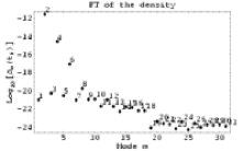
Figure 11: Same as Fig. 9 but for the $512\times 64$ resolution. The components $m\geq 19$ are set to zero because of the desaliasing process. However, the coefficients are already close to zero for $m\geq 9$ without desaliasing.

6.3 Pseudo-Schwarzschild potential

In order to take into account the modification of the radial epicyclic frequency due to the curved spacetime around a Schwarzschild black hole, we replaced the Newtonian potential by the Logarithmically Modified Potential (LMP) proposed by Mukhopadhyay (Mukhopadhyay2003 (2003)). This potential is well suited to approximate the angular and epicyclic frequencies in accretion disks around a rotating black hole. The expression of the radial gravitational field derived from this potential is then given by :

$$g_{\mathrm{r}}=-\frac{G\,M_{*}}{r^{2}}\left[1+R_{ms}\left(\frac{9}{20}\,\frac{R_{ms}-1}{r}-\frac{3}{2r}\,\ln\frac{r}{(3r-R_{ms})^{2/9}}\right)\right]$$ (64)

where $R_{ms}$ is the last stable circular orbit :

$$R_{ms} = 3+Z_{2}\pm\sqrt{(3-Z_{1})(3+Z_{1}+2Z_{2})}$$ (65)

$$Z_{1} = 1+(1-a^{2})^{1/3}\,[(1+a)^{1/3}+(1-a)^{1/3}]$$ (66)

$$Z_{2} = \sqrt{3\,a^{2}+Z_{1}^{2}}$$ (67)

The important feature of this potential is the vanishing of the radial epicyclic frequency for a single particle having a circular orbit at the innermost stable circular orbit (ISCO).

We use the same physical parameters as in the Newtonian case. The time evolution of the density perturbation in the disk is shown in Fig. 12. The Lindblad resonances are now located at $r_{\mathrm{L}}^{in/out}=21.6/45.5$ which differs slightly from the previous simulation because the orbital velocity is no more the Keplerian one but the pseudo-Newtonian one derived from Eq. (64). Here too, these locations are in agreement with the linear analysis. After a few hundreds of orbital revolutions, the disk settles down to a new quasi-stationary state, very close to the one described by the linear analysis. The profile of the density perturbation found by the numerical simulation is shown in Fig. 13 to compare with the right plot of Fig. 5. Note however that for the numerical simulations, the radial epicyclic frequency derived from the LMP Eq. (64) differs slightly from the true one given by Schwarzschild’s solution Eq. (57). As can be seen from Fig. 14, the linear regime is still a good approximation in this case, the dominant Fourier coefficient is always $m=2$.

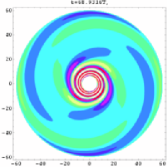
Figure 12: Final snapshot of the density perturbation in the accretion disk evolving in a perturbed pseudo-Schwarzschild potential (LMP). The disk extends from $R_{1}=6.0$ to $R_{2}=60.0$. No wave can propagate between the inner and outer Lindblad resonance.

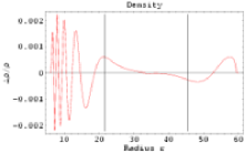
Figure 13: Same as Fig. 8 but for the pseudo-Schwarzschild geometry. The Lindblad resonances are located at $r_{\mathrm{L}}^{in/out}=21.6/45.5$.

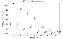
Figure 14: Same as Fig. 9 but for the pseudo-Schwarzschild geometry. The Fourier coefficients follow a decaying geometric series.

To conclude this subsection, we have shown that the introduction of the concept of ISCO in this last run does not change the qualitative conclusions drawn by the Newtonian simulations. Its only effect is to shift the location of the Lindblad resonance. This behavior was expected from the linear analysis.

6.4 Pseudo-Kerr potential

The frame dragging effect induced by the star’s rotation can also be investigated by the pseudo-Newtonian potential described in the previous section. Therefore we run a simulation in which the rotation of the star is taken into account by the gravitational field described by Eq. (64).

To create a significant change in the orbital frequency, we choose a spin parameter $a_{*}=0.5$. Thus the disk inner boundary corresponding to the marginally stable circular orbit is located at $R_{1}=4.24$. The outer computational domain is taken to be 10 times as large, at $R_{2}=42.4$.

The inner Lindblad resonance is clearly identified at $r_{\mathrm{L}}^{in}=19.2$ as can be seen from Fig. 15. The outer Lindblad resonance at $r_{\mathrm{L}}^{out}=45.8$ lies outside the computational domain and therefore does not show up in the plot, Fig. 16. The $m=2$ is the strongest mode whereas the other odd modes decrease following a geometrical series as confirmed by inspection of Fig. 17.

Here again apart from the fact that the disk approaches closer to the neutron star, the resonances behave in the same way as in the previous sections. Thus we strongly believe that the QPO phenomenon has nothing to do with any specific general relativistic effect. It just help to tune the QPO frequencies to some given values which could not be explained by a simple Newtonian gravitational potential.

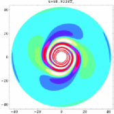
Figure 15: Final snapshot of the density perturbation in the accretion disk evolving in a perturbed pseudo-Kerr potential with $a=0.5$. The disk extends from $R_{1}=4.24$ to $R_{2}=42.4$. The outer Lindblad resonance is not in the grid.

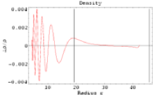
Figure 16: Same as Fig. 8 but for the pseudo-Kerr disk. The inner Lindblad resonance appears clearly at $r_{\mathrm{L}}^{in}=19.2$ while the outer one at $r_{\mathrm{L}}^{out}=45.8$ lies outside the computational grid.

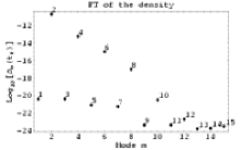
Figure 17: Same as Fig. 9 but for the pseudo-Kerr disk. Again the Fourier coefficients decay like a geometric series.

6.5 Retrograde disk

In this run, we checked that the Lindblad resonances disappear for a retrograde Newtonian disk. We rerun the simulation of subsection 6.2 by changing the sign of the spin of the neutron star by $\Omega_{*}=-0.0043311$. Thus the disk is rotating in the opposite way compared to the star.

As expected, no Lindblad resonance is observed in this run, Fig. 18. The density profile perturbation is depicted in Fig. 19 agrees well with the linear analysis, Fig. 6. A long trailing wave of mode $m=2$ expands in the whole disk area. A quasi-stationary state is reached very quickly. The Fourier spectrum behaves here again in the same manner as in the other runs Fig. 20.

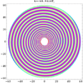
Figure 18: Final snapshot of the density perturbation in the counterrotating accretion disk evolving in a perturbed Newtonian potential. Same values as in caption of Fig. 7 applies expected for the sign of $\Omega_{*}$. A trailing spiral density wave of $m=2$ is propagating in the whole disk.

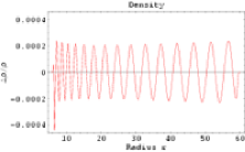
Figure 19: Same as Fig. 8 but for the counterrotating disk. No Lindblad resonances are observed.

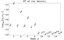
Figure 20: Same as Fig. 9 but for the counterrotating disk.

6.5.1 Wake solution in a protoplanetary disk

We also performed a set of simulations in which a Keplerian disk orbiting around a massive star $M_{*}$ is perturbed by a planet of small mass $M_{p}\ll M_{*}$. In this situation, many azimuthal modes are excited and propagate in the disk. The numerical algorithm is therefore checked when many modes are excited at the same time. The solution is represented by a one-armed spiral wake generated by the planet. In the case of weak perturbation, Ogilvie & Lubow (Ogilvie2002 (2002)) have shown that the linear response of the disk is obtained by constructive interference between wave modes in the disk. The approximate analytical shape of the wake is given by :

$$\varphi=t\pm\frac{3}{2\,\varepsilon}(\frac{r}{r_{\mathrm{c}}}^{3/2}-\frac{3}{2}\,\ln\frac{r}{r_{\mathrm{c}}}-1)$$ (68)

where $r_{\mathrm{c}}$ is the corotation radius and $t$ the time. The $+$ sign applies for the inner part of the disk ($r\leq r_{\mathrm{c}}$) while the $-$ sign applies for the outer part of the disk ($r\geq r_{\mathrm{c}}$). This result from the linear analysis is compared with the full non-linear set of Euler equations. An example is shown in Fig. 21. The non-linear simulation agrees perfectly with the linear solution given by Eq.(68) (the resolution used is $256\times 64$). A one armed spiral wave is launched from the rotating planet and propagates in the entire disk with a pattern speed equal to the rotation rate of the perturber. Several low azimuthal modes are excited to a significant level as seen in Fig. 22. However, to avoid aliasing effect because of the fast Fourier transform, we filtered out the high frequency component for $m\geq 19$. Moreover, the boundary condition imposed as non reflective waves works well by damping the perturbations close to the disk inner and outer edges.

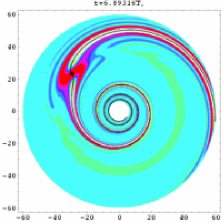
Figure 21: One-armed spiral wake generated by the orbital motion of a planet (or a small mass solid body) in the 2D accretion disk. The density perturbation $\delta\rho/\rho$ is shown. The perturbing body (like a planet) is depicted as a black circle. The linear response Eq.(68) is plotted as a solid line and overlaps well with the non-linear simulation.

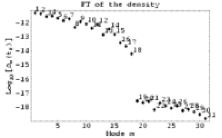
Figure 22: Same as Fig. 9 but for the wake solution.

6.6 Realistic potential

In a last run, we went back to a multipolar gravitational perturbation in the stellar disk as described in Sec. 2.3. Because the gravitational field perturbation contains several Fourier components given by the Laplace coefficients Eq. (11), many azimuthal modes are excited as in the previous case of a protoplanetary disk. For this run, the numerical values are $r_{\mathrm{p}}=5\,R_{*},z_{\mathrm{p}}=0,M_{\mathrm{p}}=10^{-3}\,M_{*}$. In order to keep a good numerical accuracy even with a system containing many modes, we increased the resolution by taking $256\times 64$. The final snapshot of the density perturbation in the disk is shown in Fig. 23. The corotation radius is clearly identified at $r=37.4$. The fluctuation in density are relevant only in the innermost region of the accretion disk where the tidal force is maximal. An inspection of the Fig. 24 confirms this remark. As seen from Fig. 25, the strongest mode is associated with $m=1$ that is the strongest exciting mode. Because the system remains in a linear regime, its total response to the perturbation is simply given by the sum of the response to each mode. This explains the decrease in the perturbed fluctuation with the mode number (see Fig. 1). Here again, the desaliasing process keeps the azimuthal modes $m\geq 19$ close to zero (within the numerical accuracy).

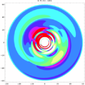
Figure 23: Final snapshot of the density perturbation in the accretion disk evolving in a perturbed Newtonian potential having many azimuthal modes $m$. The disk extends from $R_{1}=6$ to $R_{2}=60$.

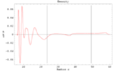
Figure 24: Same as Fig. 8 but for a perturbation containing many modes. The corotation resonance is shown by a vertical bar.

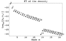
Figure 25: Same as Fig. 9 but for a perturbation containing many modes. Only the lowest Fourier modes are excited to a significant level in accordance with the perturbed potential profile.

7 DISCUSSION

The simulations presented in this paper are preliminary results mainly in order to check the numerical algorithm and to show that pseudo-spectral method are well suited to study accretion flow as was already done by Godon (Godon1997 (1997)). For smooth flows, this method shows evanescent error (exponential decrease with respect to the number of points) and good accuracy is achieved with relatively small number of discretization points.

The warping of the disk is an important processes to account for QPOs because the vertical parametric resonance locations are interesting sites to generate large amplitude in the fluctuation of the luminosity of the accretion disk. A full three dimensional linear analysis is therefore necessary to track the propagation properties of the waves in a polytropic disk. Moreover, non-linear effect are also important because in the case of magnetized accretion disk, the rotating asymmetric perturbed magnetic field is of the same order of magnitude as the background field itself. Full non-linear three dimensional numerical simulations are therefore required. The numerical code designed here can performed this task with a reasonable computational time by using only little discretization points without losing precision.

The study presented in this paper can be extended to the case of a viscous flow in the disk leading therefore to a “real accretion disk”. The viscosity will set a lower limit on the smallest scale that the density perturbation can reach. Moreover, when adding a damping term in the Mathieu equation (51) the threshold for the parametric resonance to grow will be proportional to this viscosity. We therefore expect strong oscillations only in cases where the amplitude of the perturbation is sufficiently high. In addition, the lost of energy by radiation damps these oscillations for which the kinetic energy is converted into photon emission. Finally, because the radial flux implied by the accretion process will reduce the time available for a fluid element to enter into resonance at a given radius, deviation from equilibrium will become smaller compared to a non accreting situation.

Another point not discussed in this work is the pressure induced by the radiation in the vicinity of the inner part of the accretion disk. As for the gaseous pressure, it will shift the resonance conditions derived for a single particle. A significant increase in the accretion flux induces an increase in the pressure radiation to the same order of magnitude. How the disk will react remains an open question. However it provides a correlation between the accretion rate and the orbital frequency at resonance because the resonance conditions Eq. (52)-(53)-(54) will then depend on the total pressure in the disk (gaseous + radiation).

The origin of the rotating asymmetric gravitational field for neutron stars or white dwarfs could be explained in severals ways. First, an inhomogeneous interior structure would naturally lead to the kind of potential introduced in Sec. 2.3. A second possibility is the fast rotation of the star. It leads to strong centrifugal forces deforming the star’s spherical shape into a Maclaurin spheroid. Thirdly, an aspherical star possessing a precession motion should also generate a significant distorted gravitational potential. Anisotropic magnetic stress in the stellar interior exerts also a deformation on the stellar surface which can be inferred by observation of the atmosphere. An application to white dwarfs is given by Fendt & Dravins (Fendt2000 (2000)) and for neutron star by Bonazzola & Gourgoulhon (Bonazzola1996 (1996)).

For the black hole candidates, the reason for an asymmetry in the spacetime manifold is less evident. When accreting matter, the black hole must get ride of its non-stationary state (deviation from the Kerr-Newman geometry) because of the no-hair theorem. In order to get back to its stationary state, it must emit gravitational waves described in the general relativity framework. This replaces the rotating asymmetric Newtonian potential. Like helioseismology, perturbation of the spacetime around black holes gives some insight into their properties. However, unlike asteroseismology, normal mode oscillations are unavoidably associated to gravitational wave emission. They are therefore called quasi-normal modes of the black hole because of their damping (Kokkotas & Schmidt Kokkotas1999 (1999)). If the QPOs observed in the black hole candidates could be associated with the gravitational wave emission and thus with their quasi-normal modes, we would have a new tool to explore their properties as was the case for helioseismology, a kind of “holoseismology”. This idea is discussed in Pétri (2005d ).

The discovery of high coherence in the kHz-QPOs of some systems puts strong constraints on the models. Clumps of matter cannot account for the high quality factor $Q>100$ (Barret et al. 2005a ). The coherence time involved by this picture is to long. We believe that this almost sinusoidal motion can only be imprinted by an external sinusoidal force as for instance a rotating asymmetric field would do. Moreover, sometimes, a sudden drop in this coherence is observed as was happened in 4U1636-536. Like the discrimination between slow and fast rotators (Pétri 2005b , 2005c ), it is interpreted as another manifestation of the ISCO (Barret et al. 2005b ).

8 CONCLUSION

In this paper, we have explored the consequences of a weak rotating asymmetric gravitational potential perturbation on the evolution of a thin accretion disk initially in a stationary axisymmetric state. We have shown that, when one mode is excited, the disk resonates at some radii where the resonance conditions are satisfied and reach a new quasi-stationary state in which some small scale perturbations in the density emanate starting from the inner and outer Lindblad resonance. The non wavelike disturbance rotates at the star’s spin while the free wave solutions are irrelevant because of damping process. Only the driven resonance can be maintained and account for QPOs having very high quality factors. For more general gravitational perturbation potentials, the response of the disk is the some of individual modes as long as the system remains in the linear regime. We gave a example of such a set of resonances in the last part. The physical processes at hand does not require any general relativistic effect. Indeed, the resonances behave identical in the Newtonian as well as in the pseudo-Kerr field. However, in order to get a detailed precise quantitative idea of the properties of free wave solutions and non wavelike disturbances around neutron star, we need a consistent full general relativistic description of the star-disk system. This is left for future work.

The possible warping of the disk, not discussed here, needs a full 3D analysis and simulations. We then expect some low frequency QPOs related to the kHz QPOs in a manner which has still to be determined.

We emphasize that the work presented here is a first step to a new model for the QPOs in LMXBs. A strongly non linear regime is also expected when the gravity perturbation is strong enough. The parametric resonance not developed in the simulations presented in this paper will then be excited. This is left for future work.

To conclude, to date we know about 20 LMXBs containing a neutron star and all of them show kHz-QPOs. We believe that these QPOs could be explained by a mechanism similar to those exposed here. We need only to replace the gravitational perturbation by a magnetic one as described in paper I. However, in an accreting system in which the neutron star is an oblique rotator, we expect a perturbation in the magnetic field to the same order of magnitude than the unperturbed one. Therefore, the linear analysis developed in this series of two papers has to be extended to oscillations having non negligible amplitude compared to the stationary state. We also expect the parametric resonance to become the strongest resonance in the disk. Indeed, as shown in previous work in the single particle approximation and in the MHD case (Pétri 2005b , 2005c ), the twin peak ratio of about 3/2 for the kHz-QPOs is naturally explained as well as their difference being either $\Delta\nu=\nu_{*}$ for slow rotator ($\nu_{*}\leq 300$ Hz) or $\Delta\nu=\nu_{*}/2$ for fast rotator ($\nu_{*}\geq 300$ Hz).

Finally, what would happen if we add a gravitational perturbation to a magnetic one? In the thin and weakly magnetised accretion disk, the linear analysis performed separately in the hydrodynamical as well as in the MHD case remains true when combined together. We expect again the same resonances to occur at the same locations. This is the strength of this model because it encompasses in an unique picture the white dwarf (though to be mainly in the hydrodynamical regime) and neutron star (though to be magnetised) accreting systems, explaining the 3:2 ratio whatever the nature of the compact object. In has also successfully been extended to accreting black holes by replacing these asymmetries by gravitational wave emission (Pétri 2005d ). The predicted 3:2 ratio and some lower frequency QPOs perfectly match the observations from the microquasar GRS1915+105.

Appendix A Derivation of the thin disk eigenvalue problem

In this appendix, we derive the eigenvalue problem satisfied by the radial Lagrangian displacement $\@vec{\xi}$ for a thin accretion disk for which $(H/R)\approx(c_{\mathrm{s}}/R\,\Omega)\ll 1$. We focus only on the fluid motion in the plane of the disk, no warp is taken into account, and so $\xi_{\mathrm{z}}=0$. Projecting Eq. (3.1) on the radial and azimuthal axis, we get the evolution equations for the 2D Lagrangian displacement $(\xi_{\mathrm{r}},\xi_{\varphi})$ as :

$$\rho\,\frac{\partial^{2}\xi_{\mathrm{r}}}{\partial t^{2}}+2\,\rho\,\Omega\,\left(\frac{\partial^{2}\xi_{\mathrm{r}}}{\partial\varphi\partial t}-\frac{\partial\xi_{\varphi}}{\partial t}\right)-\frac{\partial}{\partial r}\,\left(\gamma\,p\,\mathrm{div}\,\@vec{\xi}+\@vec{\xi}\cdot\@vec{\nabla}p\right)+(g_{\mathrm{r}}+r\,\Omega^{2})\,\mathrm{div}\,(\rho\,\@vec{\xi})+$$

$$\rho\,\xi_{\mathrm{r}}\,\frac{d}{dr}(r\,\Omega^{2})+\rho\,\Omega^{2}\left(\frac{\partial^{2}\xi_{\mathrm{r}}}{\partial\varphi^{2}}-2\,\frac{\partial\xi_{\varphi}}{\partial\varphi}-\xi_{\mathrm{r}}\right)=\rho\,\delta g_{\mathrm{r}}$$ (69)

$$\rho\,\frac{\partial^{2}\xi_{\varphi}}{\partial t^{2}}+2\,\rho\,\Omega\,\left(\frac{\partial^{2}\xi_{\varphi}}{\partial\varphi\partial t}+\frac{\partial\xi_{\mathrm{r}}}{\partial t}\right)-\frac{\partial}{r\,\partial\varphi}\,\left(\gamma\,p\,\mathrm{div}\,\@vec{\xi}+\@vec{\xi}\cdot\@vec{\nabla}p\right)+$$

$$\rho\,\Omega^{2}\left(\frac{\partial^{2}\xi_{\varphi}}{\partial\varphi^{2}}+2\,\frac{\partial\xi_{\mathrm{r}}}{\partial\varphi}\right)+g_{\varphi}\,(\rho\,\mathrm{div}\,\@vec{\xi}+\@vec{\xi}\cdot\@vec{\nabla}\rho)=\rho\,\delta g_{\varphi}$$ (70)

These are the two non-homogeneous equation for the Lagrangian displacement in the disk. The perturbation in the gravitational field gives rise to a driving force responsible for the non-homogeneous part. The solutions of these equations consist of free wave solutions and non-wavelike perturbations. In both cases, we are looking for solutions expressed as a plane wave in the $(\varphi,t)$ coordinates :

$$X(r,\varphi,t)=X(r)\,e^{i(m\varphi-\sigma\,t)}$$ (71)

For the non-wavelike solution, the eigenfrequency is imposed by the rotating star and is given by $\sigma=m\,\Omega_{*}$. Putting the development Eq. (71) into the system (A)-(A), we obtain :

$$(\omega^{2}-r\,\frac{d}{dr}(\Omega_{\mathrm{k}}^{2})+\Omega^{2}-\Omega_{\mathrm{k}}^{2})\,\xi_{\mathrm{r}}-2\,i\,\Omega_{\mathrm{k}}\,\omega\,\xi_{\varphi} +$$

$$c_{\mathrm{s}}^{2}\,\frac{\partial}{\partial r}(\mathrm{div}\,\@vec{\xi})+\frac{1}{\rho}\,\frac{\partial p}{\partial r}\,\left[(\gamma-1)\,\mathrm{div}\,\@vec{\xi}+\frac{\partial\xi_{\mathrm{r}}}{\partial r}\right] = -\delta g_{\mathrm{r}}$$ (72)

$$\omega^{2}\,\xi_{\varphi}+2\,i\,\Omega_{\mathrm{k}}\,\omega\,\xi_{\mathrm{r}}+\frac{i\,m}{r}\,\left(c_{\mathrm{s}}^{2}\,\mathrm{div}\,\@vec{\xi}+\frac{1}{\rho}\,\frac{\partial p}{\partial r}\,\xi_{\mathrm{r}}\right) = -\delta g_{\varphi}$$ (73)

We have introduce the following notation :

• the Keplerian angular velocity :

  $$\Omega_{\mathrm{k}}=\sqrt{\frac{G\,M_{*}}{r^{3}}}$$ (74)

• the Doppler shifted eigenfrequency :

  $$\omega=\sigma-m\,\Omega$$ (75)

• the divergence of the complex vector $\@vec{\xi}(\@vec{r})$ :

  $$\mathrm{div}\,\@vec{\xi}=\frac{1}{r}\,\frac{\partial}{\partial r}(r\,\xi_{\mathrm{r}})+\frac{i\,m}{r}\,\xi_{\varphi}$$ (76)

These are the generalization of the equations obtained by Nowak & Wagoner (Nowak1991 (1991)) in case of an external force acting on the disk. We can then solve Eq. (73) for the variable $\xi_{\varphi}$ by :

$$\xi_{\varphi}=-\frac{1}{\omega_{*}^{2}}\,\left[\delta g_{\varphi}+i\,\left(2\,\Omega\,\omega+\frac{m}{r}\,\frac{1}{\rho}\,\frac{\partial p}{\partial r}\right)\,\xi_{\mathrm{r}}+i\,\frac{m\,c_{\mathrm{s}}^{2}}{r^{2}}\,\frac{\partial}{\partial r}(r\,\xi_{\mathrm{r}})\right]$$ (77)

with $\omega_{*}^{2}=\omega^{2}-\frac{m^{2}}{r^{2}}\,c_{\mathrm{s}}^{2}$.

Substituting in the Eq. (A), the radial displacement satisfies a second order linear differential equation :

$$c_{\mathrm{s}}^{2}\,\left[1+\frac{m^{2}\,c_{\mathrm{s}}^{2}}{r^{2}\,\omega_{*}^{2}}\right]\,\frac{\partial^{2}\xi_{\mathrm{r}}}{\partial r^{2}}+\frac{c_{\mathrm{s}}^{2}}{r}\,\left[\frac{\partial\ln\,(rp)}{\partial\ln\,r}+\frac{m^{2}\,c_{\mathrm{s}}^{2}}{r}\,\frac{\partial}{\partial r}(\omega_{*}^{-2})-\frac{m^{2}\,c_{\mathrm{s}}^{2}}{\omega_{*}^{2}\,r^{2}}+\frac{m^{2}\,c_{\mathrm{s}}^{2}}{\omega_{*}^{2}\,r}\,\frac{\partial\ln p}{\partial r}+2\,\frac{m^{2}\,c_{\mathrm{s}}}{\omega_{*}^{2}\,r}\,\frac{\partial c_{\mathrm{s}}}{\partial r}\right]\,\frac{\partial\xi_{\mathrm{r}}}{\partial r}+$$

$$\left[\omega^{2}-\kappa^{2}+4\,\Omega^{2}\,\left(1-\frac{\omega^{2}}{\omega_{*}^{2}}\right)++r\,\frac{\partial}{\partial r}(\Omega^{2}-\Omega_{0}^{2})+\frac{c_{\mathrm{s}}^{2}}{r}\,(\frac{\partial\ln p}{\partial r}-\frac{1}{r})+\right.$$

$$\left.\frac{m\,c_{\mathrm{s}}^{2}}{r}\,\left(2\,\Omega\,\omega+\frac{m}{r}\,\left(\frac{c_{\mathrm{s}}^{2}}{\gamma}\,\frac{\partial\ln p}{\partial r}+\frac{c_{\mathrm{s}}^{2}}{r}\right)\right)\,\frac{\partial}{\partial r}(\omega_{*}^{-2})+\frac{\gamma-1}{\gamma\,r}\,c_{\mathrm{s}}^{2}\,\frac{\partial\ln p}{\partial r}\,\frac{m}{\omega_{*}^{2}}\,\left(2\,\Omega\,\omega+\frac{m}{r}\,\left(\frac{c_{\mathrm{s}}^{2}}{\gamma}\,\frac{\partial\ln p}{\partial r}+\frac{c_{\mathrm{s}}^{2}}{r}\right)\right)+\right.$$

$$\left.\frac{m}{\omega_{*}^{2}}\left(m\,c_{\mathrm{s}}^{2}\frac{\partial}{\partial r}\frac{c_{\mathrm{s}}^{2}}{r^{2}}+c_{\mathrm{s}}^{2}\,\frac{\partial}{\partial r}\left(\frac{2\,\Omega\,\omega}{r}+\frac{m\,c_{\mathrm{s}}^{2}}{\gamma\,r^{2}}\,\frac{\partial\ln p}{\partial r}\right)-\frac{2\,\Omega\,\omega}{r}\,\left(\frac{c_{\mathrm{s}}^{2}}{\gamma}\,\frac{\partial\ln p}{\partial r}+\frac{c_{\mathrm{s}}^{2}}{r}\right)\right)\right]\,\xi_{\mathrm{r}}$$

$$=-\delta g_{\mathrm{r}}-i\left[\left(2\,\frac{\Omega\,\omega}{\omega_{*}^{2}}-\frac{\gamma-1}{r\,\gamma}\,\frac{m\,c_{\mathrm{s}}^{2}}{\omega_{*}^{2}}\,\frac{\partial\ln p}{\partial r}+\frac{m\,c_{\mathrm{s}}^{2}}{r^{2}\,\omega_{*}^{2}}-\frac{m\,c_{\mathrm{s}}^{2}}{r}\,\frac{\partial}{\partial r}\left(\omega_{*}^{-2}\right)\right)\,\delta g_{\varphi}-\frac{m\,c_{\mathrm{s}}^{2}}{r\,\omega_{*}^{2}}\,\frac{\partial\delta g_{\varphi}}{\partial r}\right]$$

This equation can be drastically simplified in the case of a thin disk where the sound speed can be considered as a small quantity. However, in order to include properly the corotation resonance, we keep the leading terms close to the corotation radius and we have :

$$c_{\mathrm{s}}^{2}\,\left[1+\frac{m^{2}\,c_{\mathrm{s}}^{2}}{r^{2}\,\omega_{*}^{2}}\right]\,\frac{\partial^{2}\xi_{\mathrm{r}}}{\partial r^{2}}+\frac{c_{\mathrm{s}}^{2}}{r}\,\left[\frac{\partial\ln\,(rp)}{\partial\ln\,r}+\frac{m^{2}\,c_{\mathrm{s}}^{2}}{r}\,\frac{\partial}{\partial r}(\omega_{*}^{-2})\right]\,\frac{\partial\xi_{\mathrm{r}}}{\partial r}+$$

$$\left[\omega^{2}-\kappa^{2}+4\,\Omega^{2}\,\left(1-\frac{\omega^{2}}{\omega_{*}^{2}}\right)+\frac{m\,c_{\mathrm{s}}^{2}}{r}\,2\,\Omega\,\omega\,\frac{\partial}{\partial r}(\omega_{*}^{-2})\right]\,\xi_{\mathrm{r}}$$

$$=-\delta g_{\mathrm{r}}-i\left[2\,\frac{\Omega\,\omega}{\omega_{*}^{2}}-\frac{m\,c_{\mathrm{s}}^{2}}{r}\,\frac{\partial}{\partial r}\left(\omega_{*}^{-2}\right)\right]\,\delta g_{\varphi}$$ (79)

Furthermore, when far from the corotation, terms including the sound speed $c_{\mathrm{s}}^{2}$ can be neglected compared to other ones, and Eq. (A) reduces to :

$$c_{\mathrm{s}}^{2}\,\left[\frac{\partial^{2}\xi_{\mathrm{r}}}{\partial r^{2}}+\frac{\partial\ln\,(rp)}{\partial\,r}\,\frac{\partial\xi_{\mathrm{r}}}{\partial r}\right]+(\omega^{2}-\kappa^{2})\,\xi_{\mathrm{r}}=-\delta g_{\mathrm{r}}-2\,i\,\frac{\Omega}{\omega}\,\delta g_{\varphi}$$ (80)

Finally we introduce the new unknown $\psi=\sqrt{r\,p}\,\xi_{\mathrm{r}}$ to get to the same order of approximation the following Schrödinger type equation :

$$\psi^{\prime\prime}(r)+V(r)\,\psi(r)=F(r)$$ (81)

The potential is given by :

$$V(r)=\frac{\omega^{2}-\kappa^{2}}{c_{\mathrm{s}}^{2}}$$ (82)

and the source term by :

$$F(r)=-\left(\delta g_{\mathrm{r}}+2\,i\,\frac{\Omega}{\omega}\,\delta g_{\varphi}\right)\,\frac{\sqrt{r\,p}}{c_{\mathrm{s}}^{2}}$$ (83)

Eq. (81) is the fundamental equation we have to solve to find the solution to our problem far from the corotation resonance. We refer the reader to Appendix B of paper I where we develop an analytical method for approximate solutions to this Schrödinger equation.