A simple model of radiative emission in M87

Abstract

We present a simple physical model of the central source emission in the M87 galaxy. It is well known that the observed X-ray luminosity from this galactic nucleus is much lower than the predicted one, if a standard radiative efficiency is assumed. Up to now the main model invoked to explain such a luminosity is the ADAF (Advection-Dominated-Accretion-Flow) model. Our approach supposes only a simple axis-symmetric adiabatic accretion with a low angular momentum together with the bremsstrahlung emission process in the accreting gas. With no other special hypothesis on the dynamics of the system, this model agrees well enough with the luminosity value measured by Chandra.

1 Introduction

M87 is a widely studied galaxy. Many authors have written about its globular clusters and nucleus, about the hypothesis of the existence of a supermassive black hole at its centre, and recently about its jet from the nucleus (Jordán et al., 2004; Wilson & Yang, 2002). One of the most investigated problems on the physics of this galaxy is the problem of its luminosity, particularly the luminosity of its nucleus. By virtue of Chandra observations an estimate of the X-ray nuclear luminosity is about $7\cdot 10^{40}$ $erg\hskip 5.69046pts^{-1}$ (Di Matteo et al., 2003). Moreover, the data from Chandra itself allow to obtain temperature, density and radial speed profiles of the interstellar medium emitting at X-ray frequencies inside the accretion radius of the central black hole. From these quantities it is easy to calculate the Bondi accretion rate, $\dot{M}_{Bondi}=0.1\hskip 5.69046ptM_{\odot}\hskip 5.69046ptyr^{-1}$ (Di Matteo et al., 2003). Supposing a canonical radiative efficiency ($\eta=0.1$), the estimated luminosity is $5\cdot 10^{44}$ $erg\hskip 5.69046pts^{-1}$, much higher than the measured value. A common way of solving this problem is based on the assumption of the ADAF model (Chen et al., 1997) for the accreting gas. In this model a significant part of the energy produced by viscosity is advected towards the central object and therefore the fractio of gravitational energy transformed into emitted radiative energy is much lower than in the canonical Shakura-Sunyaev model (Shakura & Sunyaev, 1973). Moreover, to solve the energy excess problem, some authors have formed the hypothesis that another large part of the produced energy could be converted into the kinematic energy of the matter outflowing from the nucleus by the highly energetic jet (Wilson & Yang, 2002; Marshall et al., 2002).
In our approach, instead, we consider a steady state, axis-symmetric (with a low angular momentum) and adiabatic accretion model. Such a model, by virtue of the low value of angular momentum, is a little refinement of the standard Bondi flow. The hypothesis of an influence of core rotation on the X-ray emission in a large, slowly rotating, elliptical galaxy was already suggested by Kley & Mathews (1995). The emission process we suppose is the electron-ion thermal bremsstrahlung. This type of emission was already considered in the ADAF modeling of M87 (Ozel & Di Matteo, 2001), but not in the basic Bondi model framework. The nuclear X-ray luminosity calculated from our model is compatible with the observed value measured by Chandra. Though this model is very simple, it gives significant results with respect to the problem of the radiative emission modeling.

2 The physical model

We set up a method to fit to an experimental data (the nuclear luminosity) using a model that is compatible with the known framework about the source (whose main ingredients are: no evidence of high rotation, which implies quasi-spherical accretion, and bremsstrahlung emission process). Moreover, to perform such a kind of fit we need just one free parameter (the flow specific angular momentum), whereas the other variables are bound by the observed values at the accretion radius.
Since we will consider only small angular momentum models, we may neglect the role of viscosity. Indeed, with the low angular momentum value we will use, the gas will not rotate more than one orbit from the accretion radius to the black hole. In the presented model the rotational speed is so small that the gaseous structure is rather similar to a spherical one only slightly crushed in the vertical direction by the low angular momentum value. To obtain temperature, density and radial speed profiles we consider a set of three equations, in which the symbols used have the following meanings: $\rho$, $v$ and $a$ are respectively density, gas radial speed and sound speed, $H_{disk}$ is the half-thickness of the disk, $\dot{M}$ is the mass accretion rate, $\lambda$ is the specific angular momentum of the gas, $R_{g}$ is the Schwartzschild radius of the black hole, $\gamma=5/3$ is the ratio $c_{p}/c_{v}$ between the gas specific heats at constant pressure and volume, $\rho_{\infty}$ and $a_{\infty}$ are the density and sound speed values taken at a large distance from the black hole, in our case the values measured by Chandra at the BH accretion radius.

With these definitions, the used equation system is:

mass conservation equation:

$$4\pi rH_{disk}\rho v=\dot{M}=cost$$ (1)

radial momentum equation:

$$v\frac{dv}{dr}=-\frac{1}{\rho}\frac{dP}{dr}-\frac{GM}{(r-R_{g})^{2}}+\frac{\lambda^{2}}{r^{3}}$$ (2)

polytropic relation between density and sound speed:

$$\rho=\rho_{\infty}\left(\frac{a}{a_{\infty}}\right)^{\frac{2}{\gamma-1}}$$ (3)

Eq. 1 is the evaluation of the accretion rate $\dot{M}$ based on the idea that a mass flux $\rho v$ crosses a cylindrical surface of radius $r$ and height $2H_{disk}$, under the hypothesis that $\dot{M}$ is constant in space and time (steady accretion flow). Eq. 2 is the radial momentum transfer equation, with the lagrangian time derivative of the radial speed (without the term $\partial v/\partial t$ since we assume a steady state) in the first member and the three acting forces (pressure gradient, gravitational and centrifugal) in the second one. Eq. 3 is the thermodynamical relation between density and sound speed for an ideal gas during an adiabatic process.
The disk half-thickness is obtained through the following procedure. Using the hypothesis of vertical hydrostatical equilibrium, we can write:

$$\frac{1}{\rho}\frac{\partial P}{\partial z}=\frac{GM}{(r-R_{g})^{2}}\frac{z}{r}$$ (4)

Though the flow we analyze cannot be described as a thin disk, the only way to evaluate quantitatively the vertical height is to make this assumption. This means that we approximate the vertical gradient $\partial P/\partial z$ with $P/H_{disk}$ and substitute the $z$ value in the right hand side of eq. 4 with $H_{disk}$:

$$\frac{1}{\rho}\frac{P}{H_{disk}}=\frac{GM}{(r-R_{g})^{2}}\frac{H_{disk}}{r}$$ (5)

By some simple algebraic calculations, this leads to:

$$H_{disk}=(r-R_{g})\sqrt{\frac{P}{\rho}\frac{r}{GM}}$$ (6)

We used the Paczynsky-Wiita potential $V_{PW}=-(GM)/(r-R_{g})$ (Paczynski & Wiita, 1980) to mimic the general-relativistic gravitational effects. Note that $v>0$ for inflowing gas. The pressure $P$ is given by $P=\rho a^{2}/\gamma$.
This scheme, containing one differential and two algebraic equations, can be substituted by a totally algebraic system of equations by using the Bernoulli relation instead of the radial momentum differential equation 2:

$$\frac{v^{2}}{2}+\frac{a^{2}}{\gamma-1}-\frac{GM}{r-R_{g}}+\frac{\lambda^{2}}{2r^{2}}=B$$ (7)

where $B$ is the Bernoulli constant of the gas flow.

The algebraic equation system was solved using the following procedure. By introducing the Mach number $m=v/a$, solving for $a$ the equation 7 and putting all the terms into the relation 1, we obtained an equation in the unknown $m$:

$$\dot{M}=-r\cdot m\cdot a\cdot K\cdot a^{\frac{2}{\gamma-1}}\propto f(m)\cdot A\left(r,B,\lambda\right)$$ (8)

where $K$ is a constant depending on the entropy of the system and $f$ is function only of the Mach number:

$$f\left(m\right)=-\frac{m}{\left[\frac{m^{2}}{2}+\frac{1}{\gamma-1}\right]^{\frac{\gamma+1}{2\left(\gamma-1\right)}}}$$ (9)

and $A$ is function only of $r$ (B and $\lambda$ are parameters):

$$A\left(r,B,\lambda\right)=r\left[B-V\left(r,\lambda\right)\right]^{\frac{\gamma+1}{2\left(\gamma-1\right)}}$$ (10)

with $V\left(r,\lambda\right)$, the effective body force potential (gravitational plus centrifugal), given by:

$$V\left(r,\lambda\right)=\frac{\lambda^{2}}{2r^{2}}-\frac{GM}{r-R_{g}}$$ (11)

We used the values of density, flow radial speed and sound speed $\rho_{\infty}$, $v_{\infty}$ and $a_{\infty}$ at the BH accretion radius to calculate the Bernoulli constant $B$, necessary to solve the algebraic system. The unknowns are $\rho$, $v$ and $a$. By solving for these quantities, we obtained their radial profiles $\rho(r)$, $v(r)$ and $a(r)$. Finally, from $a(r)$ we found the temperature profile $T(r)=(m_{H}a^{2})/(2\gamma K_{B})$, where $m_{H}$ is the proton mass and $K_{B}$ is the Boltzmann constant. From the density $\rho$ and the temperature $T$ at a certain radius $r$ we calculated the emitted power density at the same $r$ for the bremsstrahlung emission process. Defining $e_{ff}$ as the emitted power density, $n_{e}$ and $n_{i}$ as the electron and ion densities in the gas, $Z$ as the atomic number of the ions, $g_{B}$ as the Gaunt factor, $e$ and $m_{e}$ as the electron charge and mass, $h$ as the Planck constant, the formula we used for bremsstrahlung is the following:

$$e_{ff}=(\frac{2\pi K_{B}}{3m_{e}})^{\frac{1}{2}}\frac{2^{5}\pi e^{6}}{3hm_{e}c^{3}}T^{\frac{1}{2}}n_{e}n_{i}Z^{2}g_{B}$$ (12)

The quantities $n_{e}$ and $n_{i}$ can be calculated from the density $\rho$ by assuming that the accreting gas is an hot plasma of fully ionized hydrogen. We adopted in our model the bremsstrahlung emission mechanism because, as already pointed out, the dominant emission process for the M87 X-ray nuclear luminosity is the thermal bremsstrahlung that yields a peak in the X-ray band (Reynolds et al., 1996). We cut off any emission when the temperature is larger than $2\cdot 10^{9}$ $K$. The main reason for the temperature cut-off is that, beyond the indicated temperature limit, the radiation frequency falls in the $\gamma$ band and therefore the nuclear emission does not contribute to the X-ray luminosity. It is clear that the procedure we followed is valid from a physical point of view if the emission process we considered does not affect very much the flow structure (we did not include the corresponding terms in the energy equation). This means that the time-scale of the process should be larger than the dynamical time of the flow. In the section 3 we show the comparison among these time-scales.
We highlight that, under the hypothesis of negligible viscosity, the algebraic method we followed is completely equivalent to the differential equation approach, since in this case the system is conservative (and the Bernoulli theorem eq. 7 holds). In particular, the algebraic method allows to find the transonic flow with the sonic point at the same radius as in the differential equation approach. In the algebraic scheme the sonic point corresponds to a minimum of $A(r,B,\lambda)$ as a function of $r$ (for the mathematical details see the Appendix of Molteni et al. (1999)), whereas in the differential equation approach the sonic point comes out from the regularity conditions on the function $v(r)$ (i.e. the usual conditions of numerator and denominator of $dv/dr$ equal to zero). For conservative systems both methods give the same results concerning the sonic point position.

3 Results

In this section we present the results obtained with a $\lambda$ value, measured in units of $cR_{g}$ (with $c$ the light speed and $R_{g}$ the Schwartzschild radius of the black hole), of 1.555, that we found to be the value of ’best fit’ of the calculated luminosity to the observed one. This value of angular momentum gives, at the black hole accretion radius, a rotational speed of 0.93 $km/sec$, that is within the observational error of the measured speed data (Cohen & Ryzhov, 1997). It is worth to note that, lowering $\lambda$, the flow structure given by our model gets closer and closer to the Bondi configuration, until, when $\lambda$ = 0, it reaches approximately the Bondi model structure. All the data shown in this section concern the range $3R_{g}<r<2\cdot 10^{5}R_{g}$, since, according to our results, it is within this region that about the $98\%$ of the total luminosity is produced. As we already pointed out in section 2, a criterion to assess the validity of our model in presence of radiative emission processes is that the flow is fundamentally adiabatic. This is verified if the emission time-scale for each considered process is larger than the flow dynamical time $t_{dyn}=r/v$ at the same radius. We present in fig. 1 the values of these typical times at different radii in the range $3R_{g}<r<2\cdot 10^{5}R_{g}$. From this figure it is clear that the bremsstrahlung emission time-scale is larger than the flow dynamical time. We do not consider the synchrotron emission because its frequency range falls in the radio and (via Comptonization) optical bands (Reynolds et al., 1996). As regards the soft X-ray emission lines, they have a significant intensity at low temperatures (about $10^{6}$ K), that can be found only beyond the accretion radius.

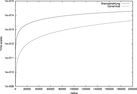
Figure 1: Comparison between the bremsstrahlung and the dynamical time-scales versus $r$. The times are in $secs$.

Our model allows to calculate the luminosity emitted by the whole flow. We present in fig. 2 the partial luminosity $L(r)$ emitted from $3R_{g}$ to a generic radius $r$. The figure shows that the largest part of the total luminosity emitted by the entire flow is produced in the region from $r=3R_{g}$ to $r=2\cdot 10^{5}R_{g}$. The luminosity coming out from the whole system (up to the external boundary at $r=5\times 10^{5}R_{g}$) is $7.1\cdot 10^{40}\hskip 5.69046pterg/sec$. Therefore our model permits to explain the observed luminosity as a result of the accretion flow emission. Obviously this picture is not the only possible one. For example, Wilson & Yang (2002) attribute the origin of the nuclear X-ray emission to the pc, or sub-pc, scale jet. However our hypothesis has the advantage of explaining the observational data in the simple framework of the interstellar medium accreting onto the central black hole.

Figure 2: Partial luminosity $L(r)$ versus $r$. $L(r)$ is in $erg/sec$.

In figs. 3, 4 and 5 we show the radial profiles of the three variables that characterize the flow structure: density, temperature and radial speed. In fig. 6 we show the radial density of the emitted power for the bremsstrahlung process.

Figure 3: Density radial profile. Density is in $g/cm^{3}$.

Figure 4: Temperature radial profile. The temperature is in $K$ degrees.

Figure 5: Flow radial speed vs. $r$. The speed is in $cm/sec$.

Figure 6: Radial density of the emitted power for the bremsstrahlung process. The power density is in $erg\cdot cm^{-1}\cdot sec^{-1}$.

4 Conclusions

In this work we show that the addition of a small gas angular momentum to a simple adiabatic accretion flow together with the thermal bremsstrahlung emission process can give, for the active nucleus of the galaxy M87, a luminosity value that is in good agreement with the measured one, whereas the value obtained supposing the standard radiative efficiency is four orders larger than the measured luminosity. We obtain this result using a very simple model that contains a new free parameter, the specific angular momentum $\lambda$ of the accreting gas, that can be adjusted in order to fit the model to the observed luminosity. With $\lambda=1.555$ the obtained luminosity value is $7.1\cdot 10^{40}\hskip 5.69046pterg/sec$ versus a measured one of about $7\cdot 10^{40}\hskip 5.69046pterg/sec$. Our result can be considered also a way of giving an estimate of the gas angular momentum in the nucleus of M87. Moreover, our model could be applied to other sources in which the low observed luminosity requires a low radiative efficiency model.

References

- Chen et al. (1997) Chen, X., Abramowicz, M. A., Lasota, J.-P., 1997, ApJ, 476, 61
- Cohen & Ryzhov (1997) Cohen, J. G., Ryzhov, A., 1997, ApJ, 486, 230
- Di Matteo et al. (2003) Di Matteo, T., Allen, S. W., Fabian, A. C., Wilson, A. S., Young, A. J., 2003, ApJ, 582, 133
- Jordán et al. (2004) Jordán, A., Côté, P., Ferrarese, L., Blakeslee, J. P., Mei, S., Merritt, D., Milosavljevic, M., Peng, E. W., Tonry, J. L., West, M. J., 2004, ApJ, 613, 279
- Kley & Mathews (1995) Kley, W., Mathews, W. G., 1995, ApJ, 438, 100
- Marshall et al. (2002) Marshall, H. L., Miller, B. P., Davis, D. S., Perlman, E. S., Wise, M., Canizares, C. R., Harris, D. E., 2002, ApJ, 564, 683
- Molteni et al. (1999) Molteni, D., Toth, G., Kuznetsov, O. A., 1999, ApJ, 516, 411
- Ozel & Di Matteo (2001) Ozel, F., Di Matteo, T., 2001, ApJ, 548, 213
- Paczynski & Wiita (1980) Paczynski, B., Wiita, P. J., 1980, A&A, 88, 23
- Reynolds et al. (1996) Reynolds, C. S., Di Matteo, T., Fabian, A. C., Hwang, U., Canizares, C. R., 1996, MNRAS, 283, 111
- Shakura & Sunyaev (1973) Shakura, N. I., Sunyaev, R. A., 1973, A&A, 24, 337
- Wilson & Yang (2002) Wilson, A. S., Yang, Y., 2002, ApJ, 568, 133