The ACS Virgo Cluster Survey IX: The Color Distributions of Globular Cluster Systems in Early-Type Galaxies

Abstract

We present the color distributions of globular cluster (GC) systems for 100 Virgo cluster early-type galaxies observed in the ACS Virgo Cluster Survey, the deepest and most homogeneous survey of this kind to date. While the color distributions of individual GC systems can show significant variations from one another, their general properties are consistent with continuous trends across galaxy luminosity, color, and stellar mass. On average, galaxies at all luminosities in our study ($-22<M_{B}<-15$) appear to have bimodal or asymmetric GC color distributions. Almost all galaxies possess a component of metal-poor GCs, with the average fraction of metal-rich GCs ranging from 15 to 60%. The colors of both subpopulations correlate with host galaxy luminosity and color, with the red GCs having a steeper slope. The steeper correlation seen in the mean color of the entire GC system is driven by the increasing fraction of metal-rich GCs for more luminous galaxies.

To convert color to metallicity, we also introduce a preliminary ($g$–$z$)-[Fe/H] relation calibrated to Galactic, M49 and M87 GCs. This relation is nonlinear with a steeper slope for ${\rm[Fe/H]}\lesssim-0.8$. As a result, the metallicities of the metal-poor and metal-rich GCs vary similarly with respect to galaxy luminosity and stellar mass, with relations of ${\rm[Fe/H]}_{MP}\propto L^{0.16\pm 0.04}\propto M_{\star}^{0.17\pm 0.04}$ and ${\rm[Fe/H]}_{MR}\propto L^{0.26\pm 0.03}\propto M_{\star}^{0.22\pm 0.03}$, respectively. Although these relations are shallower than the mass-metallicity relation predicted by wind models and observed for dwarf galaxies, they are very similar to the mass-metallicity relation for star forming galaxies in the same mass range. The offset between the two GC populations varies slowly ($\propto M_{\star}^{0.05}$) and is approximately 1 dex across three orders of magnitude in mass, suggesting a nearly universal amount of enrichment between the formation of the two populations of GCs. We also find that although the metal-rich GCs show a larger dispersion in color, it is the metal-poor GCs that have an equal or larger dispersion in metallicity. The similarity in the $M_{\star}$–[Fe/H] relations for the two populations, implies that the conditions of GC formation for metal-poor and metal-rich GCs could not have been too different. Like the color-magnitude relation, these relations derived from globular clusters present stringent constraints on the formation and evolution of early-type galaxies.

1. Introduction

Globular clusters (GCs) are found in nearly every nearby galaxy irrespective of its luminosity or gas content. The ubiquity and relative simplicity of these old star clusters makes them a fundamental tool for understanding the star formation, metal-enrichment, and merging histories of galaxies in the local universe. In particular, the color distributions of GC systems have played an important role in constraining the evolution of elliptical galaxies. While the color-magnitude diagram of early-type galaxies has garnered much interest as a strong constraint on the formation of ellipticals (e.g. Bower, Lucey, & Ellis 1992; Stanford, Eisenhardt, & Dickinson 1998), the mean color of an entire galaxy is a crude tool that necessarily combines its detailed star formation and chemical enrichment history into a single number. By comparison, globular clusters trace each major epoch of star formation, and because they are individually resolved single-age, single-metallicity systems with typical ages older than 10 Gyr, they provide a means to determine the distribution in metallicity of the early major star forming events that built their host galaxies.

Metallicity distributions of the field star populations in most nearby ellipticals are difficult or impossible to obtain with current technology, therefore the color distributions of their GC systems (inferred to be distributions in metallicity) provide the only direct probe of their chemical enrichment history. With the dichotomous nature of the Milky Way’s own GC system as a starting point (Searle & Zinn 1978), the availability of the Hubble Space Telescope (HST) over the past 15 years has enabled studies of the color distributions of extragalactic GC systems, and has revealed that bimodality is a common property in massive elliptical galaxies (Gebhardt & Kissler-Patig 1999; Kundu & Whitmore 2001). This has led to the nomenclature of blue or “metal-poor”, and red or “metal-rich” GC populations, which in the Milky Way would correspond to the halo GCs ($\langle{\rm[Fe/H]}\rangle\sim-1.59$) and the bulge/thick disk GCs ($\langle{\rm[Fe/H]}\rangle\sim-0.55$) (Côté 1999). Those dwarf elliptical galaxies that have been studied to date exhibit purely unimodal populations of metal-poor GCs (Lotz, Miller, & Ferguson 2004).

Why these color distributions should be broad or bimodal—i.e. why there should be distinct GC subpopulations—is a key issue in the quest to assemble a consistent picture of bulge, halo, and elliptical galaxy formation (see West et al. 2004 for a review). At the very least, many if not all spheroidal systems cannot have formed in a single, isolated, monolithic starburst. We see in the local universe that massive star clusters are formed wherever there is a high surface density of star formation (Larsen & Richtler 2000), and especially in major mergers (e.g. Zhang, Fall & Whitmore 2001). Thus, some proposed explanations for GC color bimodality invoke sequential episodes of star formation to create the two populations, both induced by major mergers (Ashman & Zepf 1992) and in isolation (Forbes et al. 1997). Others attempt to explain GC systems in the context of hierarchical merging with gas dissipation in both semi-analytic (Beasley et al. 2002) and hydrodynamic models (Kravstov & Gnedin 2005). While these approaches are in some ways the most promising and represent the more quantitative work applied to this problem, neither model naturally produces bimodality. Côté et al. (1998, 2000) showed that multiple star forming events were not necessary to produce bimodal metallicity distributions in a hierarchical merging framework without gas dissipation. We see evidence of this kind of gas-poor merging both locally in the form of accreted dwarf galaxies like the Sagittarius dwarf spheroidal galaxy (Ibata, Gilmore & Irwin 1995), and also in mergers of massive ellipticals in high redshift clusters (van Dokkum et al. 1999).

It is probable that aspects of all of these scenarios (which themselves are not mutually exclusive) are important for the formation of globular cluster systems. Determining the dominant mechanisms for the formation of the GC subpopulations will come from quantifying the detailed nature of these GCs. Studies of metal-poor and metal-rich GCs in individual galaxies have already shown that they have different spatial properties with the metal-rich GCs being more concentrated toward the centers of galaxies (e.g. Geisler, Lee & Kim 1996), and that they have different kinematic properties (Sharples et al. 1998; Zepf et al. 2000; Côté et al. 2001, 2003; Peng et al. 2004). Another approach to understanding GC systems, which we take in this paper, is by precisely quantifying their variation as a function of host galaxy properties. In addition, this allows us to address the similarities and differences between GCs and field stars in a systematic way, providing insight into the nature of star formation and gas flows in the early universe.

Previous studies have investigated GC color or metallicity distributions as a function of host galaxy properties. van den Bergh (1975) and Brodie & Huchra (1991) discussed the correlation between the mean metallicity of GC systems with the mean metallicity of their host galaxies. It is now well-established that more luminous and metal-rich galaxies have more metal-rich GCs. Moreover, the mean color of the metal-rich GC subpopulation also appears to correlate with galaxy luminosity. Both Forbes et al. (1997) and Kundu & Whitmore (2001) found that the colors of the metal-rich GCs correlated with host galaxy luminosity, but neither were able to detect a correlation for the metal-poor GCs. Forbes & Forte (2001) found the same to be true when the GC colors were compared to galaxy velocity dispersion.

Larsen et al. (2001) conducted a careful and homogeneous study of both GC subpopulations with deep HST/WFPC2 photometry in the F555W and F814W filters of 17 galaxies, all of which were brighter than $M_{B}=-18.6$. In the GC color distributions of these galaxies, the mean colors of both the metal-rich and metal-poor peaks increased with host galaxy luminosity. They also for the first time found that the GC system colors had a weak correlation with host galaxy color (expected because of the correlation with luminosity and the color-magnitude relation of early-type galaxies). Of particular interest lately is the degree to which the properties of metal-poor GCs are correlated with their host galaxies. The lack or weakness of any observed trends have indicated to previous authors that the metal-poor GCs must be “universal” and have formed in similar sized gas fragments under similar conditions. Burgarella et al. (2001) compiled color data on the blue GCs for 47 galaxies from the literature and found the trend to be weak or insignificant. At the other end of the galaxy luminosity function, Lotz et al. (2004) measured the GC color distributions of dwarf elliptical galaxies (dEs) using HST/WFPC2 imaging of 69 dEs in the Virgo and Fornax clusters and they too found a shallow relationship between GC color and galaxy luminosity. All of these studies relied on the best data at the time, HST/WFPC2 imaging of galaxy samples with varying degrees of heterogeneity, and almost all were based on $V$–$I$ colors. The installation of the Advanced Camera for Surveys (ACS, Ford et al. 1998) now gives us the opportunity to conduct this sort of study in a much more precise and comprehensive fashion.

The ACS Virgo Cluster Survey (ACSVCS, Côté et al. 2004, Paper I) is an HST/ACS imaging program of 100 early-type galaxies in the Virgo cluster, and is designed for studying GC systems in a deep and homogeneous manner. The breadth and depth of this survey makes it the most complete and homogeneous study of extragalactic globular cluster populations ever undertaken. Characterizing the metallicity distributions of GC systems is one of the key goals of this project. Each galaxy is imaged in the F475W and F850LP filters ($g_{475}$ and $z_{850}$), providing twice the wavelength baseline and metallicity sensitivity of the standard $V$–$I$ color. The high spatial resolution and spatial sampling of the ACS Wide Field Camera (ACS/WFC) allows us to resolve the half-light radii of GCs at the distance of Virgo, facilitating the selection of GC candidates and enabling studies of the GC sizes themselves (Jordán  et al. 2005a, Paper X). Our images also provide high precision photometry and surface brightness profiles of the galaxies themselves (Ferrarese et al. 2005, Paper VI), and their nuclei (Côté  et al. 2005, Paper VIII), as well as distances to each galaxy using the method of surface brightness fluctuations (Mei et al. 2005a,b Papers IV and V). These data have also begun to show the connection between globular clusters and ultracompact dwarf galaxies (Haşegan et al. 2005, Paper VII). Future studies (Mieske et al., in prep) will also use the ACSVCS data to address the topic of color-magnitude relations for the GCs themselves (e.g. Harris et al. 2005). Taken together, we are able to present a complete picture of these Virgo galaxies and their GC systems.

2. Data and Catalogs

2.1. Data Reduction

We have reduced our ACS/WFC images using a dedicated pipeline that is described by Jordán et al. (2004a,b, Papers II, III). Briefly, each image is combined and cleaned of cosmic rays using the Pyraf task multidrizzle (Koekemoer et al. 2002). We then create models of the galaxy in each filter for the purposes of subtracting the galaxy light. After model subtraction, we iterate with SExtractor (Bertin 1996) to mask objects, subtract any residual background, and do our final object detection using estimates of both the image noise and the noise present due to surface brightness fluctuations. Objects are only accepted if they are detected in both filters. After a selection on magnitude and ellipticity to reject obvious background galaxies, we use the program KINGPHOT (Jordán et al. 2005a) to measure magnitudes and sizes for all candidate GCs. KINGPHOT finds the best-fit King model parameters for each object given the point spread function (PSF) in that filter and at that location. Aperture magnitudes are measured on the best-fit PSF-convolved King model. For total magnitudes, we integrate the flux of the model to the limit of the PSF and apply a GC size-dependent aperture correction. This correction is determined by convolving King models of different half-light radii with both the Sirianni et al. PSF (F475W), and a PSF derived from bright stars in the Galactic globular cluster 47 Tuc (F850LP). For the purpose of measuring GC colors, we measure magnitudes within a 4-pixel radius aperture and then apply the average aperture correction for a GC with a half-light radius of 3 pc and a concentration of 1.5. The result is a catalog of total magnitudes, ($g$–$z$) colors, half-light radii ($r_{h}$) and concentrations for each object. Magnitudes and colors are corrected for foreground extinction using the reddening maps of Schlegel, Finkbeiner & Davis (1998), and extinction ratios for the spectral energy distribution of a G2 star (Paper II). In this paper, we use $g$–$z$ to mean $g_{475}$–$z_{850}$ unless explicitly stated otherwise.

Table 1Control Fields

RA(J2000)	Dec(J2000)	HST Program ID
02:06:33.85	$+20$:53:13.36	9488
02:17:20.72	$-04$:44:41.01	9488
04:40:44.48	$-45$:44:21.24	9488
09:54:35.32	$+69$:49:10.54	9575
12:10:53.82	$+39$:14:06.33	9488
12:10:33.95	$+39$:35:22.63	9575
12:25:51.14	$+00$:04:08.60	9488
12:38:32.53	$+62$:26:54.43	9488
12:43:30.12	$+11$:49:20.62	9488
13:41:40.42	$+28$:33:37.39	9488
13:53:57.73	$+69$:28:26.75	9488
15:16:15.80	$+07$:09:43.46	9488
15:43:32.26	$+59$:21:37.66	9488
15:44:50.76	$+59$:02:07.37	9488
22:12:37.23	$-83$:54:18.95	9575
22:22:57.51	$-72$:23:21.07	9488
23:46:49.49	$+12$:44:53.35	9488

2.2. Control Fields

One of the main problems with GC studies, particularly for fainter galaxies, is the contamination from background galaxies. For dwarf galaxies where there may only be a few GCs, the contamination from the background is often larger than the signal. For brighter galaxies, the light from the galaxy itself creates a spatially varying detection efficiency that complicates the comparison to blank fields. This is a problem that requires careful treatment in order to minimize systematic uncertainties, especially in low-luminosity systems.

In order to address this issue, we use archival ACS/WFC imaging of 17 blank, high-latitude fields that have been observed with the F475W and F850LP filters to the same or greater depth than our ACSVCS observations. These images were taken as part of two ACS Pure Parallel programs (GO-9488,GO-9575), and are well-suited to the purpose of understanding the background and foreground contamination in our GC samples (Table 1). Each one of these images was reduced with our pipeline in exactly the same way as our program data. Since there were no large foreground galaxies in any of the control fields, and the exposure times were longer than for our ACSVCS images, all the control data go deeper than our program data. Hence for each galaxy, we created a “custom” control sample by redoing the detection as if there was a Virgo galaxy in front of of each blank field, and each field had the same exposure time as our ACSVCS fields. To do this, we used the noise images for our program fields that are generated in the data reduction. Thus, for each control field we can produce the catalog of objects that we would have detected had the exposure times matched our ACSVCS program images, and had there been a particular ACSVCS galaxy in the foreground.

We find that using the control fields is consistent with and superior to using the local background. The degree of field-to-field cosmic variance for GC candidates in our control fields is on the order of the Poisson noise. Given our efficient selection of GC-like objects, there are not many background objects that make the cut for GC selection (see below). For example, in our faintest galaxy, VCC 1661, we only expect on average about $\sim 9\pm 4$ contaminants to the sample of GC candidates. Determining this background locally as opposed to over many control fields, while possibly more representative of the true background, introduces a large error due to counting noise of small numbers. In general, we find that the number of contaminants that we estimate from the control fields is a good match to the number of contaminants found in the dwarf galaxy fields, where the number of objects is dominated by the background (see Peng et al. 2005).

2.3. Globular Cluster Selection

The selection of a clean and complete catalog of GCs is an essential but difficult part of all GC studies. The ability to resolve and measure sizes for GCs in Virgo with HST provides much greater leverage to separate GCs from foreground stars and background galaxies. In addition, our custom control fields allow us to isolate the location of our contaminating population in the multidimensional parameter space. This efficient selection allows us to avoid stringent cuts on galactocentric radius that may strongly bias measured properties of the GC system. This approach to GC selection and background estimation makes our study particularly unique and important for the GC systems of faint galaxies where the number of GCs is small compared to the number of background galaxies. Previous studies have all required a strict selection on galactocentric radius.

While the details of the GC selection will be described in greater detail in another paper (Jordán et al. 2005b), here we briefly outline the technique. We choose a broad cut on color, selecting only objects with $0.5<g$–$z<2.0$, which generously spans the age and metallicity ranges typical of old star clusters. The strength of our selection lies in the size-magnitude diagram (Figure 1), where background galaxies are typically fainter and more extended than GCs. This figure shows the data and custom control fields for two galaxies in our sample. The custom control fields have been randomly sampled so that only $1/17$ of the objects are plotted, equivalent to what is expected for a single field. It is already well known that GCs typically have a Gaussian-like luminosity function (Harris 1991), and that the Galactic GCs have a median size of $r_{h}\sim 3$ pc. This is evident in the left hand panels of Figure 1 as a population mostly separate from the locus of background contaminants. Notice also how the custom control field includes fewer objects and is shallower for the brighter galaxy.

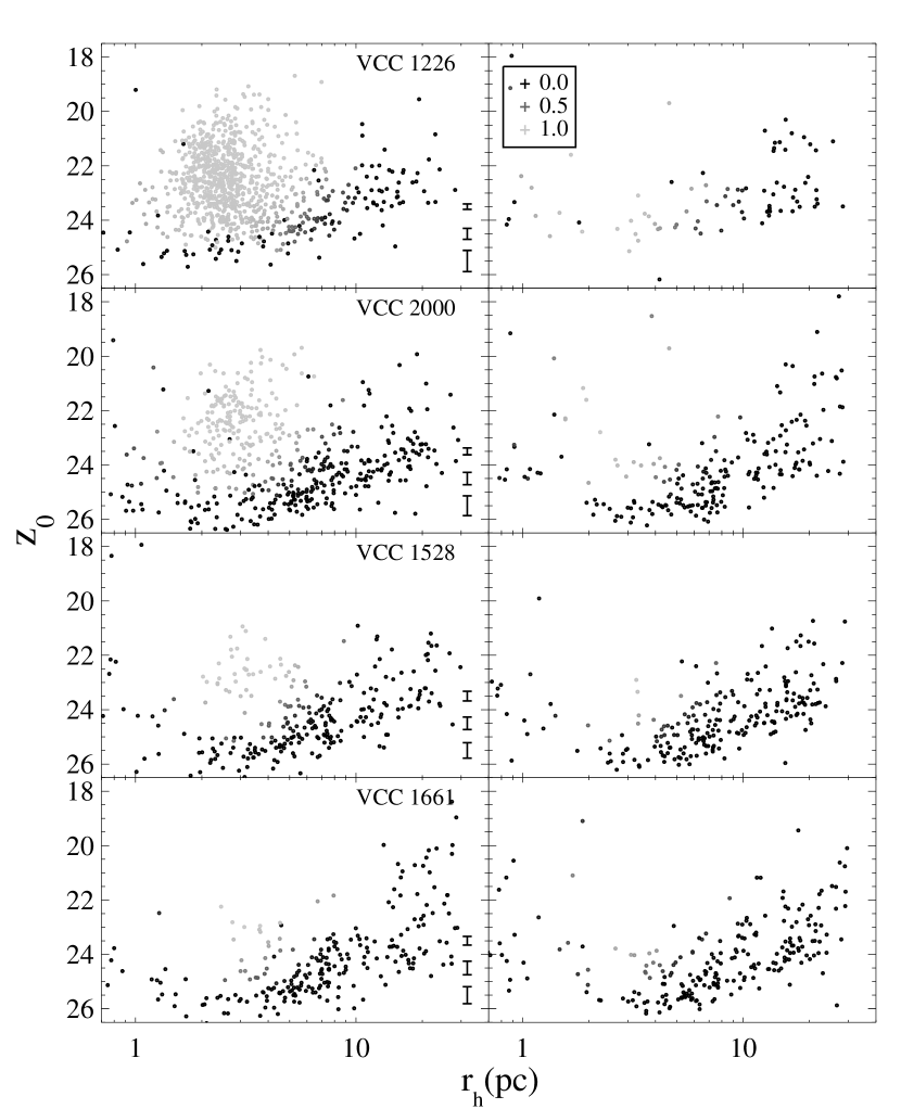
Figure 1.— Globular cluster selection diagrams for four galaxies spanning the magnitude range of our survey. From top to bottom: VCC 1226 (M49, $B=9.31$), VCC 2000 ($B=11.94$), VCC 1528 ($B=14.51$), and VCC 1661 ($B=15.97$). Left panels show the objects detected in the galaxy images. Right panels show a random selection of $1/17$ of the objects detected in 17 blank sky control fields that have been customized for the depth reached in each galaxy. Notice how the control field for VCC 1226 is shallower and has fewer objects because the galaxy is brighter and fills the frame. Object colors are coded by the probability that they are globular clusters. Error bars represent the median photometric error at those magnitudes.

We apply a Gaussian kernel to the control data to produce a nonparametric two dimensional density distribution of contaminants. We then fit a parametric model to the GC locus. In magnitude, we assume a Gaussian distribution, and in size, we use a nonparametric kernel estimate plus a power law tail, with the two joined at $r_{h}=7$ pc. This model is then fit to the data using maximum likelihood estimation — the fitting procedure allows us to account for variations in the GCLF turnover magnitude and differences in the size distributions from galaxy to galaxy. Finally, we use these two density distributions to evaluate the probability that a given object is a GC. Typically, the lines of constant probability run diagonally from the faint, compact region of the diagram to the bright, extended region (seen in Figure 1). However, even at a constant probability cut at a value of 0.5, this dividing line is not exactly the same from galaxy to galaxy. In galaxies with more GCs, it is more likely that objects in the “contaminant” locus are actually GCs, and hence they will be assigned a higher probability. For the purposes of this paper, all of our GC catalogs will use objects with GC probabilities greater than 0.5.

Recently, some investigations have revealed the existence of faint, extended star clusters in NGC 1023, NGC 3384 (Larsen & Brodie 2000; Brodie & Larsen 2002), and other nearby spiral (Chandar, Whitmore, & Lee 2004) and dwarf galaxies (Sharina, Puzia, & Marakov 2005). Because these clusters typically have similar sizes and magnitudes to background galaxies and their nature is still uncertain, our selection cuts do not include them in our GC sample and we do not include them in our analysis. Faint, extended star clusters in the ACSVCS galaxies will be treated in a separate paper (Peng et al. 2005).

3. Results

3.1. Color Distributions of Globular Cluster Systems

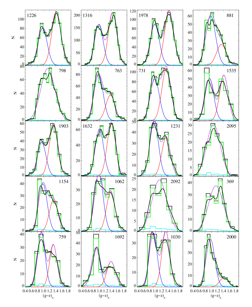
Figure 2.— Globular cluster $(g$–$z)_{0}$ distributions for all 100 ACSVCS galaxies. We plot color histograms of GC candidates (black), expected contaminants (cyan), and statistically cleaned GC distributions (green). The black curve represent a nonparametric kernel density estimate of the cleaned distribution. In cases where the distribution is likely bimodal, we plot the red and blue Gaussian components as determined by the KMM estimates, as well as their sum (purple). In the unimodal cases, we plot the best fit single Gaussian to the entire distribution (purple).

Figure 2.— continued. Globular cluster $(g$–$z)_{0}$ distributions.

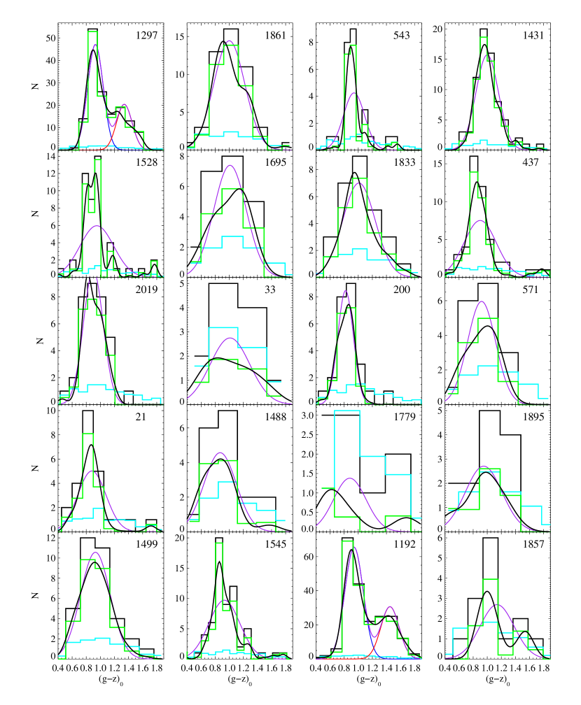
Figure 2.— continued. Globular cluster $(g$–$z)_{0}$ distributions.

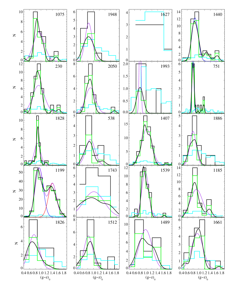
Figure 2.— continued. Globular cluster $(g$–$z)_{0}$ distributions.

Figure 2.— continued. Globular cluster $(g$–$z)_{0}$ distributions.

In Figure 2, we show the $(g$–$z)_{0}$ color distributions for the GC systems of 100 ACSVCS galaxies, ordered by decreasing total $B$ magnitude of the host galaxy. The histograms were created by binning the data with an “optimal” bin size, which is related to the width of the distribution and the total number of objects as $2IQRn^{-1/3}$, where $IQR$ is the interquartile range (the color range that includes the second and third quartile of the ranked color distribution), and $n$ is the total number of objects (Izenman 1991). The bin size is not allowed to be smaller than the mean photometric error. The histograms of the GC data are shown in black, and histograms of the expected contamination as measured from the custom control fields are shown in cyan.

While the level of contamination is negligible for the brighter galaxies, the background is a significant problem for the fainter galaxies. We create statistically cleaned samples of GCs by using a Monte Carlo procedure. For each GC, we calculate the probability that it is a contaminant by using a nonparametric density estimate of the control data as compared to the program galaxy data at that color. Based on this probability, we randomly include or do not include this object (with replacement) from our generated sample. Iterating 100 times for each galaxy, we can produce an average color distribution that is cleaned of contaminants. These histograms are plotted in green. Kernel density estimates of the cleaned distribution are overplotted as black curves.

The cleaned and smoothed color distributions show obvious bimodality for most of the brighter galaxies, something which is expected from previous investigations (e.g. Gebhardt & Kissler-Patig 1998; Larsen et al. 2001, Kundu & Whitmore 2001). For intermediate luminosities and fainter galaxies, the situation becomes less obvious as the number of GCs per galaxy decreases. Yet, it is clear that the fraction of red GCs decreases as the galaxy itself becomes fainter.

The properties of the GC color distribution are often quantified using the Kaye’s Mixture Model (KMM; McLachlan & Basford 1988; Ashman, Bird, & Zepf 1994) to fit two Gaussians to the data using the expectation-maximization (EM) method. We fit the homoscedastic case of this model, where $\sigma$ is the same for both Gaussians. Constraining $\sigma$ reduces the number of free parameters and gain leverage on noisy data in which there are generally large errors when fitting for $\sigma$ individually. We apply KMM to the each of the probabilistically cleaned GC color samples to determine the means of the blue and red peaks in the color distribution. We determine that the two Gaussian model is a better fit to the data than the one Gaussian model if the “p-value” for the bimodal model is less than 0.05. For the cases where bimodality is deemed significant ($p\leq 0.05$), Figure 2 shows the two Gaussians and their sum. For the unimodal case, the single best-fit Gaussian is plotted. In some galaxies, the distribution was determined to be bimodal, but the number of GCs in the red peak was not significant over the background at greater than 2$\sigma$. In these cases, we reject the bimodal hypothesis because the red objects are likely to be background galaxies. The results for KMM, and the parameters for the best fit one or two Gaussian models are presented in Table 2. This table includes the means of the blue and red peaks, the common sigma, the fraction of GCs that are determined to be in the red subcomponent, the total number of GCs (after accounting for the background), the p-value of the two Gaussian hypothesis and its associated error, and the mean and sigma for the entire distribution. In cases where the red peak was less than 2$\sigma$ above the background, only the mean color of the blue peak is reported. In cases where the total number of GCs was statistically equal to zero (see next section), no values could be reliably estimated.

3.2. Notes on Special Galaxies

A few galaxies are noteworthy in that they appear somewhat different from others of similar luminosity. For a more in-depth description of every galaxy in the sample, see Ferrarese et al. (2005, Paper VI). Four galaxies in particular, despite their low luminosities, have prominent blue and red peaks and have large numbers of GC. This is due to their proximity to the two giants of the cluster, M87 and M49, and we are likely observing the GC systems of their larger neighbors. Interestingly, all four are also significantly redder than one would expect for galaxies of their luminosity, and both the number and mean color of the red GCs in these galaxies is similar to those seen in galaxies of the same $(g$–$z)$ color. This suggests that they may be remnants of what were once larger, more luminous systems.

VCC1327/NGC4486A: This dwarf elliptical is only 7.5′ away from M87 (NGC 4486), and its GCs are likely to be dominated by those of the nearby cD galaxy.

VCC 1297/NGC4486B: This compact elliptical galaxy is similar to M32 in appearance, and is only 7.3′ away from M87. Some or all of its GCs may in fact belong to the M87 GC system, and its current size and luminosity may be the result of significant tidal stripping.

VCC 1192/NGC4467: This elliptical galaxy is also compact in appearance and is only 4.2′ away from M49 (NGC 4472). Its GC system may be dominated by that of M49.

VCC 1199: This elliptical is also only 4.5′ from M49. Like the other small galaxies near giant ellipticals, it displays a prominent red peak despite its low luminosity.

Other galaxies of note are:

VCC 1146/NGC4458: This galaxy is unique in the sample in that its GC system is dominated by a single red peak of GCs. The red GC fraction of 0.84 estimated by KMM is not only much larger than the value of 0.3 expected for a galaxy of this luminosity, but is much higher than the 0.6 fraction seen in the giant ellipticals.

VCC 798: This galaxy appears to be the best candidate in our sample for having a trimodal color distribution.

VCC 731: Appears to have significantly more GCs than other galaxies of comparable luminosity. The excess appears to be due to an large number of red GCs.

VCC 1692: The blue and red GCs are particularly well separated in color.

Table 2Color Distributions: Bimodal and Unimodal Parameters

No.	VCC	$\mu_{blue}$	$\mu_{blue,err}$	$\mu_{red}$	$\mu_{red,err}$	$\sigma$	$\sigma_{err}$	$f_{red}$	$f_{red,err}$	$N_{GC}$	$p$	$p_{err}$	$\mu_{1}$	$\mu_{1,err}$	$\sigma_{1}$	$\sigma_{1,err}$
(1)	(2)	(3)	(4)	(5)	(6)	(7)	(8)	(9)	(10)	(11)	(12)	(13)	(14)	(15)	(16)	(17)
1	1226	0.97	0.01	1.42	0.01	0.15	0.01	0.59	0.03	749	$<0.01$	$<0.01$	1.24	0.01	0.27	0.01
2	1316	0.98	0.01	1.43	0.01	0.14	0.01	0.56	0.02	1723	$<0.01$	$<0.01$	1.23	0.01	0.26	0.00
3	1978	0.98	0.01	1.45	0.01	0.15	0.01	0.57	0.03	791	$<0.01$	$<0.01$	1.25	0.01	0.27	0.00
4	881	0.98	0.03	1.33	0.03	0.16	0.01	0.30	0.10	353	0.01	0.02	1.09	0.01	0.23	0.01
5	798	1.02	0.02	1.34	0.03	0.17	0.01	0.37	0.09	503	0.07	0.15	1.14	0.01	0.23	0.01
6	763	0.97	0.01	1.36	0.01	0.15	0.01	0.36	0.04	489	$<0.01$	$<0.01$	1.11	0.01	0.24	0.01
7	731	0.98	0.01	1.36	0.01	0.15	0.01	0.56	0.02	889	$<0.01$	$<0.01$	1.19	0.01	0.24	0.00
8	1535	0.94	0.01	1.41	0.01	0.14	0.01	0.52	0.04	234	$<0.01$	$<0.01$	1.18	0.02	0.28	0.01
9	1903	0.94	0.02	1.33	0.01	0.14	0.01	0.61	0.03	296	$<0.01$	0.01	1.18	0.01	0.24	0.01
10	1632	1.00	0.01	1.39	0.01	0.14	0.01	0.53	0.03	437	$<0.01$	$<0.01$	1.21	0.01	0.24	0.01
11	1231	0.96	0.02	1.35	0.01	0.14	0.01	0.41	0.03	240	$<0.01$	$<0.01$	1.12	0.01	0.24	0.01
12	2095	0.92	0.05	1.22	0.04	0.16	0.02	0.53	0.16	123	0.43	0.33	1.07	0.02	0.22	0.01
13	1154	0.98	0.02	1.33	0.03	0.14	0.01	0.40	0.09	184	0.01	0.05	1.12	0.01	0.22	0.01
14	1062	0.98	0.02	1.37	0.02	0.14	0.01	0.40	0.07	169	$<0.01$	0.01	1.14	0.02	0.24	0.01
15	2092	0.94	0.04	1.33	0.04	0.15	0.02	0.50	0.08	83	0.11	0.14	1.13	0.03	0.24	0.02
16	369	0.95	0.02	1.32	0.02	0.15	0.02	0.54	0.07	170	0.07	0.13	1.15	0.02	0.24	0.01
17	759	0.93	0.02	1.32	0.02	0.12	0.01	0.44	0.07	161	$<0.01$	$<0.01$	1.10	0.01	0.23	0.01
18	1692	0.88	0.01	1.38	0.03	0.14	0.01	0.39	0.05	122	$<0.01$	$<0.01$	1.08	0.03	0.28	0.01
19	1030	0.93	0.02	1.34	0.02	0.13	0.01	0.51	0.06	165	$<0.01$	$<0.01$	1.14	0.02	0.24	0.01
20	2000	0.97	0.02	1.41	0.04	0.14	0.01	0.16	0.05	186	$<0.01$	$<0.01$	1.05	0.02	0.22	0.01
21	685	0.92	0.02	1.36	0.04	0.15	0.02	0.35	0.08	156	$<0.01$	0.01	1.07	0.03	0.26	0.02
22	1664	0.91	0.10	1.31	0.04	0.18	0.03	0.69	0.15	132	0.17	0.23	1.18	0.02	0.25	0.02
23	654	0.92	0.03	$\cdots$	$\cdots$	0.15	0.02	$\cdots$	$\cdots$	42	0.06	0.09	0.99	0.03	0.23	0.02
24	944	0.91	0.02	1.33	0.03	0.12	0.01	0.35	0.07	81	0.01	0.03	1.06	0.02	0.24	0.01
25	1938	0.92	0.04	1.36	0.14	0.16	0.02	0.17	0.09	89	0.07	0.15	0.99	0.03	0.23	0.02
26	1279	0.93	0.02	1.25	0.04	0.14	0.02	0.35	0.12	128	0.21	0.29	1.04	0.02	0.21	0.01
27	1720	0.87	0.02	1.34	0.03	0.13	0.01	0.43	0.07	64	$<0.01$	0.01	1.08	0.04	0.27	0.02
28	355	0.90	0.04	1.42	0.06	0.15	0.02	0.37	0.08	52	0.02	0.04	1.09	0.04	0.29	0.02
29	1619	0.87	0.04	1.23	0.05	0.14	0.01	0.55	0.09	56	0.19	0.21	1.06	0.03	0.23	0.02
30	1883	0.95	0.03	1.35	0.03	0.14	0.02	0.27	0.09	73	0.07	0.13	1.06	0.03	0.23	0.02
31	1242	1.00	0.05	1.44	0.17	0.15	0.03	0.28	0.16	108	0.03	0.06	1.11	0.02	0.22	0.02
32	784	1.01	0.03	1.41	0.06	0.15	0.02	0.31	0.10	55	0.15	0.17	1.14	0.03	0.24	0.02
33	1537	0.91	0.02	1.20	0.04	0.09	0.01	0.28	0.11	37	0.17	0.22	1.00	0.02	0.16	0.01
34	778	0.93	0.05	1.37	0.12	0.14	0.03	0.27	0.13	61	0.09	0.14	1.04	0.03	0.23	0.02
35	1321	0.93	0.03	1.32	0.04	0.11	0.02	0.28	0.07	43	0.02	0.04	1.04	0.02	0.21	0.02
36	828	0.89	0.02	1.29	0.04	0.11	0.01	0.29	0.05	69	0.01	0.02	1.00	0.02	0.21	0.01
37	1250	0.90	0.04	$\cdots$	$\cdots$	0.09	0.03	$\cdots$	$\cdots$	46	0.13	0.30	0.98	0.02	0.17	0.04
38	1630	0.92	0.05	1.37	0.07	0.16	0.02	0.41	0.17	46	0.17	0.21	1.10	0.03	0.27	0.02
39	1146	0.90	0.11	1.28	0.12	0.13	0.02	0.81	0.19	72	0.07	0.22	1.20	0.02	0.19	0.02
40	1025	0.90	0.08	1.31	0.15	0.14	0.02	0.16	0.19	89	0.10	0.25	0.97	0.02	0.19	0.02
41	1303	0.90	0.02	$\cdots$	$\cdots$	0.10	0.01	$\cdots$	$\cdots$	53	$<0.01$	0.01	0.94	0.02	0.17	0.03
42	1913	0.92	0.11	1.19	0.09	0.14	0.03	0.36	0.21	56	0.45	0.40	1.02	0.03	0.19	0.02
43	1327	0.92	0.02	1.34	0.03	0.14	0.01	0.34	0.05	161	$<0.01$	$<0.01$	1.06	0.02	0.24	0.01
44	1125	0.88	0.02	1.19	0.14	0.13	0.02	0.16	0.16	53	0.34	0.36	0.93	0.02	0.17	0.02
45	1475	0.86	0.08	1.19	0.22	0.12	0.02	0.27	0.27	76	0.33	0.34	0.94	0.02	0.16	0.02
46	1178	0.93	0.04	1.33	0.08	0.14	0.02	0.32	0.12	80	0.02	0.03	1.06	0.03	0.23	0.02
47	1283	0.94	0.03	1.29	0.08	0.13	0.03	0.25	0.09	56	0.21	0.30	1.03	0.03	0.21	0.03
48	1261	0.99	0.09	$\cdots$	$\cdots$	0.13	0.03	$\cdots$	$\cdots$	37	0.21	0.41	1.05	0.03	0.19	0.04
49	698	0.90	0.15	1.33	0.24	0.15	0.03	0.30	0.31	108	0.14	0.25	1.00	0.02	0.19	0.02
50	1422	0.87	0.26	1.21	0.19	0.15	0.05	0.51	0.40	29	0.38	0.44	1.09	0.04	0.19	0.04
51	2048	0.92	0.02	$\cdots$	$\cdots$	0.06	0.01	$\cdots$	$\cdots$	16	0.02	0.06	1.01	0.04	0.17	0.03
52	1871	0.88	0.02	$\cdots$	$\cdots$	0.06	0.01	$\cdots$	$\cdots$	13	0.08	0.22	0.96	0.05	0.17	0.05
53	9	0.91	0.03	$\cdots$	$\cdots$	0.10	0.03	$\cdots$	$\cdots$	27	0.01	0.07	1.01	0.06	0.25	0.07
54	575	0.88	0.03	1.21	0.05	0.09	0.02	0.36	0.14	19	0.14	0.20	1.00	0.05	0.18	0.02
55	1910	0.92	0.15	1.51	0.30	0.18	0.05	0.29	0.30	47	0.15	0.19	1.06	0.03	0.25	0.03
56	1049	0.75	0.11	$\cdots$	$\cdots$	0.13	0.04	$\cdots$	$\cdots$	11	0.36	0.32	0.97	0.08	0.27	0.05
57	856	0.96	0.03	$\cdots$	$\cdots$	0.11	0.01	$\cdots$	$\cdots$	42	$<0.01$	0.01	1.02	0.03	0.21	0.04
58	140	0.83	0.10	1.15	0.08	0.11	0.02	0.50	0.25	21	0.35	0.26	1.00	0.04	0.18	0.03
59	1355	0.69	0.13	$\cdots$	$\cdots$	0.14	0.04	$\cdots$	$\cdots$	12	0.41	0.29	0.92	0.07	0.26	0.05
60	1087	0.87	0.11	1.29	0.32	0.13	0.02	0.24	0.30	59	0.31	0.40	0.94	0.02	0.16	0.03
61	1297	0.93	0.01	1.34	0.03	0.11	0.01	0.30	0.04	142	$<0.01$	$<0.01$	1.05	0.02	0.22	0.01
62	1861	0.91	0.05	1.35	0.22	0.15	0.03	0.25	0.12	39	0.27	0.32	1.00	0.04	0.22	0.03
63	543	0.89	0.07	$\cdots$	$\cdots$	0.07	0.03	$\cdots$	$\cdots$	19	0.08	0.21	0.94	0.04	0.15	0.06
64	1431	0.96	0.03	$\cdots$	$\cdots$	0.12	0.02	$\cdots$	$\cdots$	63	0.16	0.26	1.00	0.02	0.16	0.02
65	1528	0.89	0.02	$\cdots$	$\cdots$	0.12	0.03	$\cdots$	$\cdots$	41	0.10	0.31	0.95	0.03	0.24	0.04
66	1695	0.76	0.09	1.19	0.06	0.11	0.03	0.58	0.22	14	0.20	0.25	1.01	0.06	0.23	0.04
67	1833	0.90	0.09	$\cdots$	$\cdots$	0.14	0.03	$\cdots$	$\cdots$	20	0.29	0.31	1.01	0.05	0.23	0.04
68	437	0.83	0.09	$\cdots$	$\cdots$	0.12	0.03	$\cdots$	$\cdots$	38	0.10	0.31	0.90	0.04	0.23	0.05
69	2019	0.76	0.14	1.00	0.08	0.09	0.04	0.48	0.29	27	0.33	0.37	0.90	0.03	0.14	0.02
70	33	0.79	0.12	$\cdots$	$\cdots$	0.11	0.04	$\cdots$	$\cdots$	5	0.78	0.36	1.01	0.16	0.28	0.10

Table 2Color Distributions: Bimodal and Unimodal Parameters

No.	VCC	$\mu_{blue}$	$\mu_{blue,err}$	$\mu_{red}$	$\mu_{red,err}$	$\sigma$	$\sigma_{err}$	$f_{red}$	$f_{red,err}$	$N_{GC}$	$p$	$p_{err}$	$\mu_{1}$	$\mu_{1,err}$	$\sigma_{1}$	$\sigma_{1,err}$
(1)	(2)	(3)	(4)	(5)	(6)	(7)	(8)	(9)	(10)	(11)	(12)	(13)	(14)	(15)	(16)	(17)
71	200	0.69	0.11	0.89	0.08	0.07	0.03	0.63	0.28	18	0.33	0.30	0.82	0.03	0.11	0.02
72	571	0.69	0.08	$\cdots$	$\cdots$	0.09	0.02	$\cdots$	$\cdots$	11	0.26	0.26	0.92	0.06	0.20	0.04
73	21	0.75	0.10	$\cdots$	$\cdots$	0.09	0.03	$\cdots$	$\cdots$	17	0.20	0.31	0.88	0.05	0.20	0.07
74	1488	0.72	0.10	$\cdots$	$\cdots$	0.10	0.05	$\cdots$	$\cdots$	10	0.22	0.27	0.87	0.07	0.23	0.08
75	1779	0.66	0.08	$\cdots$	$\cdots$	0.11	0.06	$\cdots$	$\cdots$	2	0.99	0.07	0.88	0.34	0.23	0.27
76	1895	0.69	0.19	$\cdots$	$\cdots$	0.11	0.05	$\cdots$	$\cdots$	6	0.56	0.39	0.95	0.11	0.26	0.08
77	1499	0.82	0.08	1.18	0.18	0.14	0.03	0.39	0.28	27	0.41	0.32	0.93	0.04	0.21	0.03
78	1545	0.90	0.02	$\cdots$	$\cdots$	0.17	0.03	$\cdots$	$\cdots$	53	0.14	0.33	0.93	0.02	0.22	0.03
79	1192	0.94	0.01	1.45	0.03	0.13	0.01	0.32	0.05	200	$<0.01$	$<0.01$	1.10	0.02	0.28	0.01
80	1857	0.99	0.05	$\cdots$	$\cdots$	0.07	0.02	$\cdots$	$\cdots$	8	0.17	0.33	1.14	0.09	0.24	0.07
81	1075	0.82	0.16	$\cdots$	$\cdots$	0.11	0.05	$\cdots$	$\cdots$	20	0.14	0.31	0.93	0.04	0.19	0.05
82	1948	0.72	0.06	$\cdots$	$\cdots$	0.05	0.02	$\cdots$	$\cdots$	6	0.67	0.37	0.83	0.06	0.12	0.04
83	1627	$\cdots$	$\cdots$	$\cdots$	$\cdots$	$\cdots$	$\cdots$	$\cdots$	$\cdots$	0	$\cdots$	$\cdots$	$\cdots$	$\cdots$	$\cdots$	$\cdots$
84	1440	0.87	0.04	$\cdots$	$\cdots$	0.11	0.02	$\cdots$	$\cdots$	31	$<0.01$	0.02	0.98	0.04	0.25	0.04
85	230	0.84	0.11	$\cdots$	$\cdots$	0.11	0.03	$\cdots$	$\cdots$	31	0.09	0.27	0.92	0.04	0.21	0.05
86	2050	0.79	0.06	$\cdots$	$\cdots$	0.06	0.02	$\cdots$	$\cdots$	13	0.22	0.28	0.89	0.06	0.17	0.10
87	1993	$\cdots$	$\cdots$	$\cdots$	$\cdots$	$\cdots$	$\cdots$	$\cdots$	$\cdots$	2	$\cdots$	$\cdots$	$\cdots$	$\cdots$	$\cdots$	$\cdots$
88	751	0.80	0.01	$\cdots$	$\cdots$	0.03	0.01	$\cdots$	$\cdots$	15	0.05	0.20	0.85	0.04	0.12	0.04
89	1828	0.73	0.16	0.97	0.12	0.08	0.03	0.61	0.39	20	0.30	0.41	0.88	0.03	0.11	0.03
90	538	0.75	0.08	$\cdots$	$\cdots$	0.07	0.03	$\cdots$	$\cdots$	5	0.69	0.41	0.89	0.09	0.16	0.09
91	1407	0.96	0.06	$\cdots$	$\cdots$	0.13	0.03	$\cdots$	$\cdots$	49	0.12	0.27	1.02	0.02	0.18	0.03
92	1886	0.70	0.05	$\cdots$	$\cdots$	0.04	0.02	$\cdots$	$\cdots$	6	0.58	0.43	0.80	0.05	0.11	0.03
93	1199	0.94	0.02	1.40	0.02	0.14	0.01	0.41	0.04	216	$<0.01$	$<0.01$	1.13	0.02	0.27	0.01
94	1743	0.75	0.19	$\cdots$	$\cdots$	0.13	0.07	$\cdots$	$\cdots$	7	0.46	0.40	1.01	0.17	0.36	0.10
95	1539	0.90	0.07	$\cdots$	$\cdots$	0.06	0.02	$\cdots$	$\cdots$	34	0.13	0.21	0.97	0.02	0.12	0.04
96	1185	0.85	0.03	$\cdots$	$\cdots$	0.12	0.02	$\cdots$	$\cdots$	26	0.10	0.22	0.92	0.04	0.21	0.03
97	1826	0.66	0.07	$\cdots$	$\cdots$	0.08	0.03	$\cdots$	$\cdots$	8	0.35	0.34	0.76	0.07	0.18	0.06
98	1512	0.63	0.11	$\cdots$	$\cdots$	0.06	0.02	$\cdots$	$\cdots$	9	0.27	0.33	0.82	0.06	0.15	0.04
99	1489	0.83	0.04	1.22	0.05	0.09	0.02	0.40	0.16	16	0.12	0.20	0.98	0.05	0.22	0.03
100	1661	0.75	0.17	$\cdots$	$\cdots$	0.09	0.05	$\cdots$	$\cdots$	12	0.19	0.29	0.95	0.06	0.20	0.08

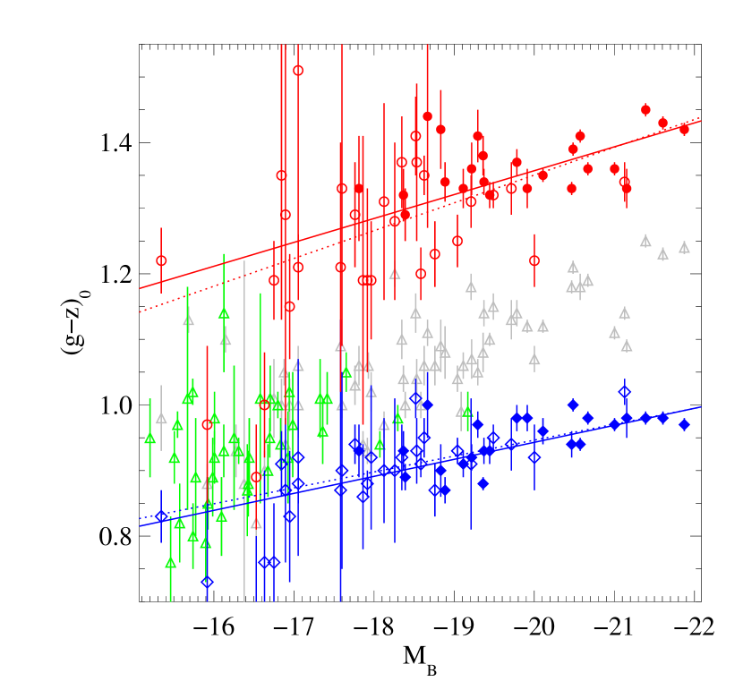
Figure 7.— Mean colors of the entire GC system and the two GC subpopulations as a function of $M_{B}$. We plot the values of the blue and red means as determined by the KMM algorithm assuming a model of two Gaussians with a common dispersion. Only 54 galaxies for which the red peak was more than 2-sigma above the background are plotted with two peaks (circles and diamonds). Filled symbols represent the 24 galaxies that have significant bimodal distributions ($p<0.05$), and the solid lines are fits to these points. Open symbols are for the 30 galaxies with $0.05<p<1$ and the dotted lines are fit to data of all p-values. The means of the entire GC color distribution are also plotted (green and gray triangles) with 46 of the points (green) representing the GC systems determined to be unimodal in color.

VCC 1499: While this galaxy appears to be an elliptical on ground based Digitized Sky Survey images, our ACS images reveal it to contain numerous young blue star clusters at the center. Also, the color of the galaxy is one of the bluest in the sample, suggesting that it may be a dI/dE transition object. In the same field, only 1.4′ away, is a true dE, VCC 1491, hence the clusters measured in this field are a combination of the systems of these two galaxies.

VCC 9: This galaxy has a very low surface brightness for its reported luminosity.

VCC 1938: This S0 galaxy is 1.7′ from the neighboring nucleated dE, VCC 1945. We detect GCs in both galaxies, although there are many fewer associated with VCC 1945 as it is $\sim 2.5$ mag fainter.

VCC 33, 1779, 1627, 1993: In the full field data for these galaxies, the number of GC candidates we detect is less than 3$\sigma$ above the expected background. VCC 1779 shows spiral structure and dust, is likely to have a younger age, and there are a two likely star clusters near the center. The other three galaxies do not show any obvious concentrations of GCs at their centers although there may be one or two GCs in each galaxy. Only for VCC 1627 do we not detect any GC candidates above the background.

For the purposes of the analysis that follow, we exclude from our sample the galaxies VCC 1327, 1297, 1192, 1199 (near giants), 1499, 1779 (younger ages), and 1938 (two galaxy blend) because either the detected globular cluster systems may not be representative of the targeted galaxy, or the young ages belie the classification as an early-type galaxy. This leaves us with 93 galaxies in our sample.

3.3. GC colors and Host Galaxy Properties

3.3.1 Color Decompositions of Individual GC Systems

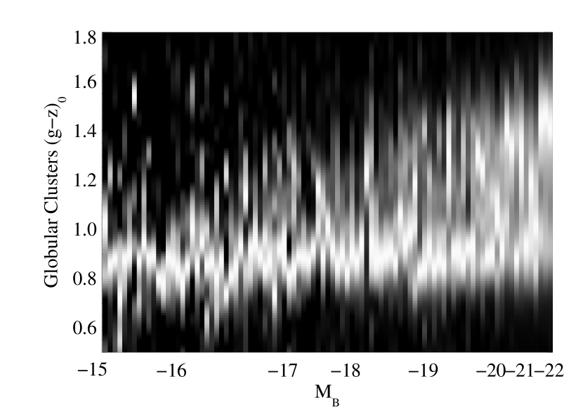
Figure 8.— This image shows the GC color distributions of the ACSVCS galaxies ordered by host galaxy $M_{B}$. Each column is a kernel density estimation of a galaxy’s GC color distribution, with white normalized to represent the peak density. The galaxies are ordered in increasing luminosity from left to right. The image shows that all galaxies seem to possess a population of blue GCs with similar color, but that the color and relative fractions of red GCs is a strong function of galaxy luminosity.

Using the mixture model estimates presented in Table 2, we can investigate the behavior of the blue and red GC subpopulations as a function of galaxy luminosity. Previous studies along these lines were mainly based on HST/WFPC2 data (Forbes et al. 1997, Kundu & Whitmore 2001; Larsen et al. 2001; Burgarella et al. 2001) and included very few galaxies with $M_{B}$ fainter than $-19.5$. The study of Lotz et al. (2004) targeted dEs in Virgo and Fornax, and saw no evidence for bimodality in their GC color distributions. The higher metallicity sensitivity of the ($g$–$z$) color and the deeper photometry of our ACS observations makes this an ideal program for testing these relationships in a homogeneous fashion across a wide range of galaxy luminosities and colors.

In Figure 7, we show the mean colors of the blue and red GC subpopulations as a function of the absolute blue magnitude of their host galaxy. The galaxy magnitudes are from the photometry of Binggeli, Sandage & Tammann (1985) and are listed for the entire sample in Paper I. We assume a distance to the Virgo cluster of 16.5 Mpc (Tonry et al. 2001) with a distance modulus of $31.09\pm 0.03$ mag from Tonry et al. (2001), corrected by the final results of the Key Project distances (Freedman et al. 2001; see also discussion in Mei et al. 2005b). The GC color data follow Table 2, and the two individual means are plotted for all galaxies that had a significant ($>2\sigma$) red GC population. For 24 galaxies plotted as solid points, the distributions were significantly bimodal ($p\leq 0.05$). The color distributions for 30 other galaxies (open points) can also be decomposed into two components, but are less uniquely described by a two-Gaussian model ($0.05<p\leq 1$). In both cases, we plot the means of the two fitted Gaussians only if the number of red GCs is more then 2$\sigma$ above the expected background. This eliminates small numbers of red background galaxies from causing spurious bimodality. For the remaining 46 galaxies (those that have insignificant numbers of red GCs), we treat them as unimodal and plot the means of their entire GC color distributions (triangles).

We are able to resolve the GC subpopulations for galaxies $\sim 2$ mag fainter than those in previous studies, and we observe a clear trend that the mean colors of both blue and red GCs are redder for more luminous host galaxies, and that the slope of the relation for red GCs is steeper by a factor of 1.6–1.9. We fit these relations to both the $p<0.05$ sample and the full sample, deriving the following weighted linear fits of the form

$$\langle g-z\rangle=a+b\times M_{B}$$ (1)

Coefficients for these fits are listed in Table 4. While most galaxies with $M_{B}<-18$ have distinguishable blue and red components in their GC color distributions, the fraction of galaxies whose distributions are not well resolved increases for fainter galaxies until all of the galaxies with $M_{B}>-16$ have an insignificant number of red GCs. Because both the fraction of red GCs and the total number of GCs is lower for fainter galaxies, the red subpopulation becomes more difficult to separate out at intermediate luminosities. However, the slopes that we derive from the brighter galaxies are statistically identical to those fit to the larger sample. In other words, even when a galaxy’s GC color distribution is not statistically very different from unimodal, a decomposition into two components is still consistent with the trends seen in more luminous galaxies, and thus may still be an appropriate description of the system.

3.3.2 Color Distributions Binned by Galaxy Properties

Figure 9.— Kernel density color distributions of GCs in seven bins of host galaxy magnitude (a) and six bins of host galaxy $(g$–$z)_{0}$ (b). Magnitude bins are 1 mag wide and extend from $M_{B}=-21$ to $M_{B}=-15$ (red to blue). The distance to the Virgo cluster is assumed to be 16.5 Mpc. Bins of color are 0.1 mag wide from 1.6 to 1.1, with the last bin extending to 0.75 (red to blue). Distributions have been corrected for the expected background and foreground contamination as measured from our control fields. All color distributions have been constructed with a Gaussian kernel ($\sigma=0.05$ mag). Notice how even the faintest and bluest bins in our sample appear asymmetric, indicating the presence of some red GCs. Data for this plot is listed in Tables 5 and 6

When the data is of high enough quality, it is sometimes best to view the data itself in aggregate rather than struggle with parametrization. Figure 8 displays a nonparametric representation of the GC color distributions for 92 galaxies (the 93 from our analysis sample minus VCC 1627, which has no detected GCs). Each column of this plot is the background cleaned color distribution of a single galaxy’s GCs constructed with a Gaussian kernel, where the grayscale has been scaled such that zero density is black and the mode of the distribution is white. The galaxies are rank ordered by their luminosity with approximate $M_{B}$ labeled on the x-axis. Immediately apparent from this image are the two GC subpopulations and their behavior with galaxy luminosity. Nearly all galaxies appear to possess a blue subpopulation of GCs, and the mean of this population varies only slowly with galaxy luminosity. In addition, there is a population of red GCs whose color and number fraction increase in a continuous fashion across our entire sample, spanning seven magnitudes of galaxy luminosity. Lotz et al. (2004) made a similar inference when comparing the GCs in dEs to the blue GCs in ellipticals. Interestingly, a red wing in the GC color distribution appears to exist even in some of our faintest galaxies, although the small number of GCs and increased noise due to background subtraction makes it difficult to quantify this for any individual galaxy.

Figure 8 displays the utility of grouping galaxies together by their intrinsic properties. Because of the large number of galaxies in our sample, we can quantify trends by treating the galaxies collectively even when any single faint galaxy has too few GCs for substantive analysis. In Figure 9, we investigate the GC color distributions as a function of both galaxy luminosity and galaxy color by binning them and accumulating enough GCs to overcome the noise. We create seven bins of magnitude from $M_{B}=-22$ to $-15$ in steps of one magnitude. We have six bins in galaxy color, five from $(g-z)_{0}=1.6$ to $1.1$ in steps of 0.1 mag, and the last bin somewhat larger $0.75<(g-z)_{0}<1.1$. The colors of the galaxies were derived from our ACS images as described in Paper VI. Briefly, the colors were estimated by directly integrating the observed surface brightness profiles between 1$\arcsec$ and the smaller of one effective radius or the radius at which the surface brightness profile falls one magnitude below the sky (in either filter).

The cumulative background cleaned GC color distributions for these galaxy bins are presented in Figure 9. The trends seen in Figure 8 are also evident in the first plot of Figure 9. In each color distribution a strong blue peak is easily visible, and each distribution is asymmetric about this blue peak, even the one for our faintest bin. The behavior of the red peak is also easy to discern. The number fraction and color of the red peak progressively decreases for fainter galaxies. Where the red peak is obvious, it also appears to be broader than the blue peak. The same progression is seen for bins in galaxy color. Redder galaxies have more red GCs, and these red GCs are themselves redder.

Each of the magnitude and color bins across our entire sample possess a population of blue GCs with some additional red GCs. We can try to decompose these two populations in our binned sample in a way similar to how we treated the individual galaxies, by treating them as the sum of two Gaussian distributions. However, given the higher signal-to-noise of these summed distribution, we find that the sum of two Gaussians, whether with identical or independent variances, is often not a good model for the color distributions for the purpose of measuring the colors of the two modes. When we run the KMM algorithm on these data to test for bimodality, all the color distributions return small $p$-values, including the faintest and bluest bins. However, when estimating the mean values of the blue and red GC peaks, the two-Gaussian fits systematically skew the colors of the blue and red peaks toward the median of the entire distribution—i.e. the estimated color of the blue peak is too red, and the estimated color of the red peak is too blue as compared to a non-parametric estimation from the data. This effect is most pronounced when the modes are of nearly equal strength, and the result is to introduce a bias that is correlated with galaxy luminosity or color. This is something that needs to be treated with care because it can produce correlations that are merely artifacts of the parameter estimation.

3.3.3 Nonparametric Decompositions of Binned GC Color Distributions

While the addition of another Gaussian component (and its attending free parameters) does improve the fit with marginally significant $p$-values in some cases, we instead choose to avoid this somewhat arbitrary model and decompose the two peaks in a nonparametric way. Given the ubiquity of the blue GCs, we start with the assumption that every color distribution is made up of a population of blue GCs with a symmetric distribution about the blue mode. We then take the GCs blueward of the blue mode, reflect them about the blue mode, and take that to be the blue GC population. The remainder of the GCs are then what we consider the red GCs. The peak color of the red peak is estimated from the GC color distribution that has the blue GCs subtracted. While this method does make assumptions, particularly about the symmetry of the blue GC color distribution and the choice of a kernel size, unlike a multi-Gaussian model it makes no assumptions about the shape of the red GC color distribution. The results are also not particularly sensitive to the size of the kernel as long as it is not so small as to introduce spurious peaks, and not so large as to be comparable to the half-width of the blue peak.

Figure 10.— Color histograms and nonparametric decompositions of GCs binned by host galaxy magnitude.

In Figures 10 and 11, we overplot our nonparametric decompositions for the GC color distributions, binned by galaxy magnitude and color. We estimate the median color and the half-width that encompasses 68% of the GCs for each peak, and also for the entire GC population in that bin. The parameters and their errors for this model were estimated using the bootstrap with 1000 iterations. These values are listed in Tables 5 and 6.

Figure 11.— Color histograms and nonparametric decompositions of GCs binned by host galaxy color.

Using these decompositions, we can study the properties of the GC color distribution as a function of galaxy properties. The results of these fits are shown in Figures 12-14. In Figure 12a we show the relationship between the median colors of the red, blue, and total GC populations against galaxy luminosity and galaxy color. As in Figure 7, the colors of the red, blue, and total GC populations correlate with the luminosity of the host galaxy. The coefficients for the linear fits are presented in Table 7. The relationship versus luminosity is similar to that shown with individual galaxies in Figure 7. However, there are two notable differences. First, we are able to trace the mean colors of the red and blue peaks for the entire magnitude range of our sample with much less noise. Second, the slopes of the red and blue relations are more disparate than they are in Table 4. The slope for the red GCs is steeper and the slope for the blue GCs is shallower than was derived from individual galaxies. The result is that the slope for the red GCs is 4.6 times steeper than for the blue GCs.

Why would the two different methods give different values? This difference stems from two effects. The first is that the individual galaxy and binned galaxy data were decomposed using two different methods. When we apply the KMM algorithm to the binned data, we do get a steeper blue GC relation and a shallower red GC relation. However, as we noted before, this is at least in part due to biases in the fitting of the peaks that arises from non-Gaussianity in the underlying distributions. While a homoscedastic two-Gaussian fit is often the best one can do for the GCS of a single galaxy, the binned data provide a more critical test of an inadequate model, and also make nonparametric methods more feasible.

The second reason for the difference is that the GC systems of individual galaxies sometimes cannot be decomposed into two populations, either because they have no red GCs, the number of red GCs has low significance, or the total number of GCs is simply insufficient. These galaxies are necessarily dropped, thus biasing the data toward galaxies with well-spaced GC subpopulations. This is a bias that will be strongest at the faint end of the galaxy luminosity function, and will result in a shallower slope for the red GCs and a steeper slope for the blue GCs. The binned data includes all galaxies, regardless of their individual decomposition, and thus is less biased in this fashion.

Figure 12b also shows the relationship between the colors of these peaks with the color of the galaxy. The bluest bin is somewhat suspect as it contains few galaxies and is quite noisy. The other bins, however, each contain $\gtrsim 400$ GCs. Both of the GC subpopulations show a clear correlation with galaxy color, with the red GCs showing a steeper relation. Larsen et al. (2001) found that the two peaks correlate with galaxy color at the 2–$4\sigma$ level (see their note added in manuscript), and the higher precision of the ACS photometry for both the GCs and the galaxies leaves little to doubt. While this relationship might be expected since galaxy color is known to correlate with luminosity, the color-magnitude relationship for galaxies has significant scatter at the faint end (see Ferrarese et al. 2005) and it is not obvious that a tight correlation should necessarily exist. The coefficients of the weighted linear fits are given in Table 7. The dashed line in this plot shows the one-to-one relation between host galaxy and GC colors. For bright galaxies, the median color of the entire GC system appears to track the galaxy color closely with a $\sim 0.3$ mag offset, but the slope changes for faint galaxies.

Figure 12.— Mean values of blue, red, and total GC colors as a function of host galaxy luminosity (left) and color (right). Magnitude and color bins, are the same as in Figure 9. Points represent the blue peak of the GC color distribution (blue diamonds), the red component (red filled circles), and the mean of the entire distribution (asterisks). The dotted lines are linear fits to the two subpopulations, and the dashed line (right) has slope unity and represents the galaxy colors. Both populations of GCs get redder with galaxy luminosity and color, but the slope for the red GCs is many times steeper.

Figure 13.— Color dispersions ($s_{68}$, the 68% half-width) of blue (diamond), red (dot), and total (asterisk) GC distributions as a function of host galaxy luminosity (left) and color (right) binned by magnitude. Magnitude, and color bins same as in Figure 9. For luminous and red galaxies, the width of the red subpopulation appears to be larger that that for the blue GCs.

In Figure 13, we show the fitted color dispersion in each subpopulation, and the dispersion of the entire color distribution as a function of galaxy luminosity and galaxy color. In both plots, we can see that the dispersion in the GC colors increases for more luminous and redder galaxies. Although most work on individual galaxies necessarily assume that the widths of the blue and red distributions are the same, these decompositions for our binned distributions shows that, at least for the brighter galaxies, the dispersion in color of the two populations may not in fact be the same but that the red GCs may have a larger spread in color. We note that the way we have chosen to do our nonparametric decomposition, the width of the blue GC distribution is entirely dependent on the half of that is blueward of the peak. However, KMM estimates of the dispersions using a heteroscedastic Gaussian model give a similar result.

One of the other noticeable trends across galaxy luminosity and color involves the fraction of red GCs. Figure 9 shows how the fraction of red GCs is much higher in more luminous and redder galaxies. We quantify this in Figure 14, showing that even in the faintest bin in our sample, galaxies on average have a $\sim 15\%$ fraction of red GCs, and this increases to $\sim 60\%$ for the most luminous galaxies. In the most luminous galaxies, however, we are only sampling the inner regions of the GC system and color gradients could slightly affect the total fractions (see e.g. Rhode & Zepf (2004) for a wide-field study). Nevertheless, This changing fraction of red GCs is the main driver behind the correlation between the mean color for the entire system and the luminosity of host galaxy.

Figure 14.— Fraction of red GCs as a function of host galaxy luminosity, binned by magnitude. The fraction of red GCs increases by over a factor of six across the magnitude range of our sample.

4. Discussion

4.1. The ($g$–$z$)–[Fe/H] Relation for Globular Clusters

In order to make inferences on the nature of GCs and their host galaxies, it is necessary to translate observables (color, magnitude) into physical properties (metallicity, luminosity, mass). One of the more critical transformations is that of color to metallicity for globular clusters. Because GCs are old, simple stellar populations, broadband color should be a good proxy for metallicity. Beyond an age of a few Gyr, the color of a star cluster is predominantly determined by its metal content, and because it was formed in a single burst, there is no complicated star formation history to disentangle. However, in practice, determining the precise transformation from different filter systems to [Fe/H] even for this simplest of stellar populations is a difficult task.

Evolutionary synthesis models of stellar populations can in theory produce these relations, but broadband colors provide a challenge as they are highly dependent on the spectrophotometry of the input stellar libraries, whether theoretical or empirical. Recent models (e.g. Bruzual & Charlot 2003) show reasonable agreement with Milky Way, M31, and Magellanic Cloud star clusters. Others have taken an empirical approach and fit various relationships to the measured colors and metallicities of GCs in the Milky Way and other nearby systems. The color used most often is $V$–$I$ and numerous relations have been calibrated, although their slopes can vary by a factor of two (Couture, Harris, & Allwright 1990; Kissler-Patig et al. 1997; Kissler-Patig et al. 1998; Kundu & Whitmore 1998; Barmby et al. 2000). All of these calibrations rely heavily on the Milky Way GCs (although Kissler-Patig 1998 includes GCs from NGC 1399 to supplement the metal-rich end). The main limitations of this approach are the homogeneity of the Galactic GC photometry, the accuracy of the published reddenings, and the inherent sensitivity of the $V$-$I$ color to metallicity. Moreover, models predict that the color-metallicity relationship should be nonlinear, especially for metal-poor populations where metallicity sensitivity in the optical is diminished.

Figure 15.— [Fe/H] versus $(g$–$z)_{0}$ for 40 low-extinction Milky Way GCs, 33 M49 and M87 GCs with ACSVCS photometry, and 22 M49 and M87 GCs with SDSS photometry. All GCs have published spectroscopic metallicity determinations as described in the text. The relatively low scatter in the data compared to previous work shows that the relation is very likely non-linear, with a steepening at ${\rm[Fe/H]}<-0.8$. The dotted line is a broken linear bisector fit to all GCs with ${\rm[Fe/H]}<0$.

The color that we are working with, ($g$–$z$), is twice as sensitive to metallicity as $V$-$I$ (Paper I), and thus offers higher metallicity resolution than previous studies. Because of the importance of deriving this transformation, we have completed a program to image the Milky Way GC system in these two bandpasses in order to derive an empirical ($g$–$z$)–[Fe/H] relation. We used the Cassegrain Focus CCD Imager on the CTIO 0.9-meter telescope over two observing runs (8 May – 12 May 2003 and 31 May – 6 June 2004) to observe $\sim 100$ Milky Way GCs in the $g^{\prime}$ and $z^{\prime}$ filters. We present a preliminary color-metallicity relation in this section, while the details and final analysis of this data set will be presented in a separate paper (West et al., in prep).

From a sample of 76 Milky Way GCs with good photometry, we selected 40 that have low reddenings of $E(B-V)<0.3$. Reddenings and [Fe/H] values for these GCs were obtained from the McMaster Milky Way GC catalog (Harris 1996) with reddenings and metallicities predominantly compiled from Reed, Hesser, & Shawl (1985), Webbink (1985), Armandroff & Zinn (1988), and Zinn (1985). To supplement this sample, especially at higher metallicities, we added GCs in the giant ellipticals M87 and M49 that have spectroscopic metallicities (Cohen, Blakeslee, & Ryzhov 1998; Cohen, Blakeslee, & Côté 2003). The latter metallicities were measured using models of Worthey (1994) and calibrated to the metallicity scale of Zinn & West (1984). For 33 of these GCs, we have ($g_{475}$–$z_{850}$) colors from our ACS/WFC photometry. For another 22, we were able to retrieve $g_{SDSS}$ and $z_{SDSS}$ photometry from the Sloan Digital Sky Survey Third Data Release (Abazajian et al. 2005), and correct them for reddening from the maps of Schlegel et al. (1998). All photometry was shifted to the HST/WFC AB photometric system ($g_{475}$ and $z_{850}$).

In Figure 15, we show the combined sample of 95 globular clusters with both a metallicity determination and a ($g$–$z$) color. While there is still sizable scatter in the data, the relation is tight enough to show a significant departure from linearity with the relation steepening for [Fe/H]$<-1.0$. The dotted line shows a broken linear fit to the data, with a break point of ($g$–$z$)$=1.05$. Because there is appreciable scatter in both axes, we fit the relation as both [Fe/H] vs. ($g$–$z$) and ($g$–$z$) vs. [Fe/H], and take the mean of the results (e.g. Barmby et al. 2000). We take this approach because there is both intrinsic and observational scatter in both variables, and the scatter is not well-quantified. We also fit the data using an ordinary least squares bisector fit and the method of bivariate correlated errors with intrinsic scatter (BCES; Akritas & Bershady 1996). We find that both of these methods give similar results, with the slopes varying by less than $4\%$ depending on the chosen method, a range much smaller than the error (see also Isobe et al. 1990 for a discussion of linear regression methods). Our fit does not include the GCs with [Fe/H]$>0$. Not only are the Worthey (1994) models not well-calibrated in that regime, but the mean colors of the red GCs that we are concerned with in this paper always have ($g$–$z$)${}_{0}<1.5$.

The relation we derive is:

$${\tiny{\rm[Fe/H]}=\left\{\begin{array}[]{ll}-6.21+(5.14\pm 0.67)(g_{475}-z_{850}),&\mbox{$0.70<(g_{475}-z_{850})\leq 1.05$}\\ -2.75+(1.83\pm 0.23)(g_{475}-z_{850}),&\mbox{$1.05<(g_{475}-z_{850})<1.45$}\end{array}\right.}$$ (2)

Figure 16.— [Fe/H] versus $(g$–$z)_{0}$ for Milky Way, M49, and M87 GCs (as in Figure 15) with stellar population models. For each model we plot the [Fe/H] and $(g$–$z)_{0}$ values for a 13 Gyr simple stellar population (black points, linearly interpolated). The solid purple line is the broken linear bisector fit from Figure 15. While the models show decent agreement with the data, there is a large spread at low metallicity, and there are also no models for metallicities in the crucial range $-0.6<{\rm[Fe/H]}<-1.6$.

In Figure 16, we show the same data and the broken linear fit, but plot predicted colors from three different models with different initial mass functions (IMF). We choose the high resolution models of Bruzual & Charlot (2003) with IMFs of Chabrier (2003) and Salpeter (1955), the 2001 release of the Bruzual & Charlot (1993) models, and the PÉGASE models, Version 2 (Fioc & Rocca-Volmerange 1997) with both Salpeter and Kroupa (2001) IMFs. In all cases, we have linearly interpolated the model data (black points) for a 13 Gyr old simple stellar population. While there is decent agreement between the models at metallicities [Fe/H]$>-1$, the relations are increasingly in disagreement at lower metallicities, and the steepness of the relation makes the choice of IMF an important one. Additionally, the lack of model isochrones for $-1.6<{\rm[Fe/H]}<-0.7$ means that there is little information on the color-metallicity relation for a range that is crucial for GCs, and where the slope of the relation is rapidly changing. Because of this, we will adopt our preliminary empirical relation to obtain metallicities in this paper. Nevertheless, we urge caution to all who would transform GC colors into metallicities using either theoretical or empirical relations.

Lastly, we note that by using the Milky Way GCs to calibrate the color-metallicity relation, we are assuming that all globular clusters have old ($>10$ Gyr) ages. This, however, may not be the case in all GC systems. For example, spectroscopic age determinations of metal-rich GCs in a few other galaxies show that some of them can have intermediate ages of 3–8 Gyr (Goudfrooij et al. 2001; Peng et al. 2004; Puzia et al. 2005). For the trends we see in color to be caused solely by age trends, though, would require that the red GCs in our faintest galaxies have a mean age of 3 Gyr, assuming that the GCs in the most massive galaxies were 13 Gyr old. While this mean age is unlikely given the current data, it is not out of the question that smaller galaxies may have somewhat younger metal-rich GCs. The age difference necessary for the blue GCs would be smaller (7 Gyr old in our faintest bin). However, all spectroscopic evidence to date indicates that metal-poor GCs in nearby galaxies have ages that are consistent with those of the Galactic GC system. Thus, we will assume that the Milky Way GCs can provide a good calibration for extragalactic GCs with the caveat that if there is a trend for less luminous or bluer galaxies host younger GCs, it will serve to flatten the relations we derive for metallicity.

4.2. Globular Cluster Metallicities, Galaxy Luminosity, and Stellar Mass

Using our empirical color-metallicity relation, we can transform the colors of the binned GC populations to [Fe/H]. In Figure 17, we plot the metallicities of the blue, red, and total GC populations against the host galaxy $M_{B}$. The coefficients for the linear fits to these relations are presented in Table 7. As was suggested by Figure 12a, the metallicities of both the metal-rich and metal-poor GC populations increase for more luminous host galaxies. One noticeable difference from Figure 12a, however, is that the slope of the relation for the metal-poor GCs is more pronounced, and is similar to the slope for the metal-rich GCs. Given the ($g$–$z$)-[Fe/H] relation in equation 2, the metallicity of the GC populations are proportional to a power of the luminosity as $Z\propto L^{\alpha}$ where $\alpha=0.16\pm 0.04,\ 0.26\pm 0.03,\ {\rm and}\ 0.52\pm 0.02$ for the metal-poor, metal-rich, and total GC populations. These errors include the formal errors in the color-metallicity relation. Lotz et al. (2004) fit the relation to the $V$–$I$ colors of the total GC populations in Virgo and Fornax dEs (assuming only a single component), and their slopes were $Z\propto L^{0.16\pm 0.05}\ {\rm to}\ L^{0.22\pm 0.05}$ depending on whether they included Local Group dwarf spheroidals or the blue GCs from Larsen et al. (2001). This is in reasonable agreement with our fits especially considering that our sample galaxies are generally more massive, and that they used both a different color and color-metallicity relation.

One of the most fundamental galaxy properties is its mass. While we do not have dynamical masses for these galaxies yet, we can obtain a rough estimate of its stellar mass-to-light ratio from its broadband optical-infrared colors. We use our ($g$–$z$) colors and $J$-$K$ from the Two Micron All Sky Survey Extended Source Catalog. These colors and magnitudes are listed in Paper VI. Although these galaxies likely have complex star formation histories that complicate the determination of $M/L_{B}$, we can obtain a crude estimate by comparing their colors to simple stellar population model grids. We use the Bruzual & Charlot (2003) models to obtain an average luminosity-weighted $M/L_{B}$ for each galaxy. We then create seven logarithmic bins of mass and nonparametrically decompose the GC populations. These values are listed in Table 8.

Figure 17.— Mean metallicities of blue, red, and total GC populations as a function of galaxy luminosity. Bins and points are the same as for Figure 12. The asterisk represents the spheroidal component of the Milky Way (bulge and halo) and its GC system.

Figure 18 shows the relationship between the metallicity of the GC subpopulations and galaxy stellar mass. Similar to the previous figure, the metallicities of both GC subpopulations correlate strongly with galaxy mass. Across nearly four orders of magnitude in stellar mass, we find that $Z\propto M_{\star}^{\beta}$ where $\beta=0.17\pm 0.04,\ 0.22\pm 0.03,\ {\rm and}\ 0.41\pm 0.01$ for the metal-poor, metal-rich, and total GC populations.

The more obvious manifestation of the correlation in the metal-poor GCs is due to the nature of the ($g$–$z$)-[Fe/H] relation, which steepens for bluer/metal-poor stellar populations. One implication of this is that it is a difficult task to tease out any differences between metal-poor clusters using broadband colors, and that the apparent universality of the population (at least in metallicity) may be in part due to photometric errors, small numbers of GCs, or the use of a less sensitive color such as $V$-$I$. Almost all previous studies on this topic have also used linear color-metallicity relations in either $V$–$I$ or $C$–$T_{1}$.

Larsen et al. (2001) derive slopes between $V$–$I$ and $M_{B}$ of $-0.016\pm 0.005$ and $-0.020\pm 0.008$ for the blue and red GCs, respectively. If we convert these to [Fe/H] using the relation of Barmby et al. (2000), which has a slope of 4.22, then this gives $\alpha=0.17\ {\rm and}\ 0.21$ for  the blue and red GCs. As with the slopes we derived with KMM on individual galaxies, the blue GCs have a slightly steeper, and the red GCs a slightly shallower slope than what we finally derive with the binned sample. However, given the differences in sample, filters, and the assumption of a linear color-metallicity relation, the comparison can be considered consistent.

Figure 18.— Mean metallicities of blue, red, and total GC populations as a function of galaxy stellar mass. Stellar mass has been translated from luminosity using an average, luminosity-weighted mass-to-light ratio. Data for this plot is in Table 8.

We emphasize, however, that the significances of the correlations are independent of the color-metallicity relation. It is the exact values of these proportionalities, especially the one for the metal-poor GCs, that are critically dependent on the adopted ($g$–$z$)-[Fe/H] relation. We illustrate this in Figure 19, in which we plot the various linear fits for the $M_{B}$-[Fe/H] data assuming different transformations from ($g$–$z$) to [Fe/H]. The models we use are the same as those in Figure 16, and as in that Figure we linearly interpolate the models. While the slopes for the metal-rich GCs are all very similar, the slopes for the metal-poor GCs can vary by a factor of three. However, one bit of independent reassurance is visible in Figures 17 and 19 where the large asterisk represents the Milky Way spheroid (bulge and halo), and its associated metal-rich and metal-poor populations of globular clusters. We take the luminosity of the Galactic spheroid to be $M_{B}=-19.19$ from Côté (1999). That these values are close to what we might predict from the relations derived for Virgo ellipticals is interesting in itself, and lends credibility to our empirical color-metallicity transformation.

4.3. The Formation and Evolution of Globular Cluster Systems

Our ability to characterize the GC metallicity distributions across a large range of galaxy masses provides a clearer and more precise view of the nature of globular cluster systems. The continuity of GC system properties that we see paints a picture in which the formation and evolution of GC systems shares a common mechanism across all galaxies. Other properties of GC systems are also either constant or slowly varying, such as the luminosity function, the size distribution (Jordán et al. 2005a), and the GC formation efficiency—globular clusters make up 0.25% of the baryonic mass of a galaxy (McLaughlin 1999). This continuity mirrors the structural properties of the galaxies themselves, which show them to be part of a continuously varying single family (Ferrarese et al. 2005, Paper VI; Côté et al. 2005, Paper VIII).

Figure 19.— Linear fits to the [Fe/H]-$M_{B}$ relations assuming different transformations from $(g$–$z)_{0}$ to [Fe/H]. We show fits using different models with different IMFs as well as our empirical broken linear fit to the Galactic GC data. While the slope of the relation in the red GC metallicity regime is generally robust across different assumed transformations, the slope of the blue GC relation can vary by a factor of three.

The correlations of the mean metallicities of metal-poor and metal-rich GCs with galaxy mass, luminosity, and color show that the formation of both subpopulations are closely linked to their parent galaxies. The nearly universal presence of a metal-poor population points to an era of star formation that was ubiquitous in the early universe at or shortly after reionization. Even at that early epoch—one associated with an epoch of “halo formation”—the metallicities of the forming star clusters are directly affected by the depth of the potential well that will eventually host the GC system. The metal-rich GCs appear to be associated with the formation of bulges and ellipticals—the metal-rich spheroid that defines the Hubble sequence in the local universe. Their numbers correlate strongly with the mass of the spheroid, indicating that they may have formed in the same events. Comparisons between GC and planetary nebula kinematics also support this view (Peng et al. 2004).

The relationship between the mean metallicity of a stellar system and its mass is a record of the enrichment and merging that occurred. There is a well established mass-metallicity relationship for the field stars of dwarf galaxies (e.g. Dekel & Woo 2003) and for the gas phase abundance of normal galaxies (Tremonti et al. 2004). Supernova wind feedback and its associated loss of metals has been used to explain the $Z\propto M^{0.4}$ relationship for Local Group dwarfs (Dekel & Silk 1986) and can reproduce the flattening of this relationship at higher mass. In their high-resolution simulations, Kravstov & Gnedin (2005) find their simulated galaxies to have $Z\propto M^{0.5}$. Although we know little about the epoch of halo formation, it is possible that galaxy outflows also play a role in enriching and triggering the formation of globular clusters (Scannapieco, Weisheit & Harlow 2004). Do these relationships apply to GC systems, and should they?

Interestingly, we find $Z\propto M^{0.41}$ for the total GC systems of our sample galaxies. This may just be a coincidence since the slope is driven by the fraction of metal-rich GCs and hence must flatten at lower masses to follow the metal-poor relation. Moreover, it is in the dwarf regime where $\alpha=0.4$ is seen for the field stars, not for more massive galaxies. However, if we assume that the metal-poor and metal-rich GCs were formed in different events then we might expect that their individual $\alpha$ values would reflect the global metallicities of their host galaxies. In the mass range that we are concerned with ($10^{9}$ to $10^{12}M_{\sun}$), the slope of the $M_{\star}$–$Z$ relationship for galaxies is significantly shallower than $\alpha=0.4$. Fitting the effective yield data for the SDSS galaxies presented in Table 4 and Figure 8 of Tremonti et al. (2004), we find that in this mass range $Z\propto M^{0.19}$, which is quite similar the relation for both GC subpopulations, and is also significantly shallower than the relation seen for Local Group dwarf galaxies. This suggests that star formation and feedback in both the epochs of halo and metal-rich spheroid formation may not have been too different from each other or from that observed in the present day. In addition, we find that the Milky Way’s total spheroid falls neatly on our relations derived for Virgo ellipticals. While there are some dependencies between the two samples because our color-metallicity relation was partly calibrated using Galactic GCs, the luminosity of the spheroid is independent. This agreement suggests that spheroids and GC systems in disk galaxies may form in much the same was as cluster ellipticals, although a large census of GC systems in disk galaxies will be necessary to explore such issues.

The slopes of the mass-metallicity relationships are surprisingly similar for metal-rich and metal-poor GCs. One consequence of this is a nearly constant offset between the metallicities of the two populations across nearly three orders of magnitude in mass, $\Delta{\rm[Fe/H]}\propto M_{\star}^{0.05}\sim 1\ {\rm dex}$. If the two populations are formed in different star forming events, this offset could point to a characteristic enrichment that is attained between starbursts.

Recent studies of galaxies in general point to the existence of a bimodality in galaxy properties about a “characteristic mass” of $3\times 10^{10}M_{\sun}$ (Kauffmann et al. 2003). Galaxies with higher masses tend to be spheroids with old stellar populations, and those with lower masses are likely to be star-forming disks. This bimodal rather than continuous distribution of galaxy properties may have its roots in the details of gas inflow and outflow, or feedback from active galactic nuclei (Dekel & Birnboim 2005). For the GC systems, the only property that appears to change at this mass scale is the fraction of red GCs, which is nearly constant above this mass, and drops quickly below it. This reinforces the idea that the metal-rich GCs are linked to the formation of the metal-rich spheroid. This characteristic mass is also the regime at which the mass-metallicity relation of star forming galaxies appears to flatten (Tremonti et al. 2004). It is interesting to note then, although perhaps not entirely surprising since our sample consists only of early-types, that this characteristic mass does not appear to be important for the mass-metallicity relationships of GC systems. All galaxies appear to possess some old, GC-like stellar population, regardless of mass, gas content, or Hubble type (see Chandar, Whitmore, & Lee 2004, Olsen et al. 2004 for GCs in spiral galaxies and Seth et al. 2004 for dwarf irregulars). More observations are necessary to determine whether the GC systems of disk galaxies other than the Milky Way are consistent with the same trends we see in this study, but if they are then it would point to a scenario where the processes that are affected by this characteristic mass scale occur after (or independently from) the formation of the GC system. This is further supported by the constant offset in metallicity between GCs and the field stars of $\sim 0.8$ dex that has been observed across a large range of galaxy luminosity (Jordán et al. 2004c). We speculate that this could be because massive star clusters form early in a star formation episode and are less affected by the subsequent feedback-related effects that shape the main body of the galaxy.

With larger numbers of GCs in our sample allowing us to study galaxies in bulk, we choose to defer debates over whether a single GC system is unimodal, bimodal, or multimodal. Occasional claims for multimodality have been made for specific galaxies (in particular because of a population of intermediate-age metal-rich clusters), although it is very difficult to tease out such effects with single color data alone. In our data, we assess that VCC 881 and 798 show color distributions that are potentially multimodal, but the occurrence is otherwise rare or too difficult to discern. While there are always individual galaxies with unique GC systems, the general trends are unmistakable. GC color distributions are on average bimodal or asymmetric down to the magnitude limit of our sample, $M_{B}\sim-15$. Almost all galaxies have a population of metal-poor GCs, the mean metallicity of which increases with galaxy mass. These galaxies also possess some number of more metal-rich GCs whose number fraction and mean metallicity are also strong functions of galaxy mass.

Figure 20.— Metallicity dispersions (68% half-width) for the red and blue GC populations. Dispersions were calculated using the color dispersions and transforming them to metallicity using the proper branch of the ($g$–$z$)-[Fe/H] relation. Note that although the red GCs had a larger dispersion in color (Figure 13), the steeper slope of the color-metallicity relation in the blue results in the blue GCs having the larger dispersion in metallicity.

The metallicity dispersions of GC systems increases rapidly for more massive galaxies, and this is largely driven by the increasing fraction of the red GCs. When comparing the metallicity dispersions of the red and blue GCs, the red GCs in massive galaxies do seem to have larger dispersions in color than the blue GCs, a factor of 1.3 in the mean. However, the shallower slope (i.e. increased metallicity sensitivity) of the ($g$–$z$)–[Fe/H] relation at ${\rm[Fe/H]}>-0.8$ means that they do not translate into larger dispersions in metallicity. In fact, the slope of the color-metallicity relation is $2.8\pm 0.5$ times steeper for metal-poor clusters, which means that it is the metal-poor GCs that have the larger dispersion in metallicity. This is illustrated in Figure 20, where the median dispersion is $0.53\pm 0.07$ dex for the metal-poor GCs, and $\sim 0.29\pm 0.04$ dex for the metal-rich GCs, where the errors reflect the formal errors in the slope of the ($g$–$z$)-[Fe/H] relation.

The dispersion in metallicity potentially tells us something about the degree of gas mixing that occurred during galaxy formation. A large metallicity dispersion could be caused by prolonged formation in a single galaxy, or also by a combination of star formation events that are chemically isolated from each other (whether spatially or temporally) and that only merge together after star formation has ceased. This latter scenario could apply to both metal-poor globular clusters that formed from isolated gaseous fragments in the early universe, or to metal-rich clusters that form during the hierarchical build up of the metal-rich spheroid. It will be interesting to see whether the lack of a larger dispersion in the metal-rich GCs, if confirmed, poses a problem for secondary formation scenarios that require the red GCs to be the product of multiple star forming events at moderate to low redshift, or if the metallicity resolution is still inadequate to resolve these effects. A narrower dispersion in metallicity also suggests that the metal-rich population may be formed in few large starforming events where the gas is well mixed.

Naturally, this inference is highly dependent on the color-metallicity relation, but we point out that none of the models shown in Figure 16 will produce a larger dispersion for the metal-rich GCs. At best, the two populations have the same dispersion. The Milky Way GC system does not show such a large dispersion difference between the metal-poor and metal-rich GCs, however, and so we will likely need the final ($g$–$z$)-[Fe/H] calibration before we can verify this intriguing result.

5. Conclusions

Ever since the launch of $HST$, the color distributions of extragalactic globular cluster systems have provided a unique window onto the evolution of elliptical galaxies. In this paper we present the globular cluster color distributions in ($g$–$z$) of 100 early-type galaxies from the ACS Virgo Cluster Survey. As the largest sample of its kind, studied with the increased sensitivity and spatial sampling of the $ACS/WFC$, and with the $g_{475}$ and $z_{850}$ bandpasses, this is one of the definitive data sets for extragalactic GC studies. We use carefully constructed control fields to account for galaxy specific and spatially varying foreground and background contamination. We also use a new size-magnitude algorithm to produce a clean sample of GCs. Using both two-Gaussian models and a nonparametric decomposition of the color distributions, we measure the characteristics of the traditional metal-poor and metal-rich subcomponents of the GC systems. We also present a preliminary transformation from ($g$–$z$) to [Fe/H] using the colors of Galactic GCs, as well as GCs in M49 and M87. Our main conclusions are:

1. While the color distributions of individual galaxies can show significant variations from one another, their general properties are consistent with continuous trends across galaxy luminosity, color, and mass. Both dwarf and giant ellipticals appear to be subject to the same family of processes that drive the formation and evolution of GC systems.

2. Galaxies at all luminosities in our study, on average, appear to have bimodal or asymmetric GC color distributions. All galaxies have a system of blue GCs with an average color around $g$–$z\sim 0.9$ and a red component whose fraction varies with the luminosity or color of the galaxy. When decomposed into blue and red GC subpopulations, the red GCs on average compose $\sim 15\%$ of the GCs in the faintest and bluest galaxies in our sample ($M_{B}=-16$, $g$–$z=1.0$), and up to 60% of the GCs the brightest and reddest galaxies ($M_{B}=-21$, $g$–$z=1.5$).

3. The colors of the blue and red GC subpopulations correlate with the luminosity and color of the host galaxy. In ($g$–$z$), the slope determined for the red GCs is 4.6 times steeper than for the blue GCs.

4. The color and metallicity widths of the entire GC system increases with galaxy luminosity and color. The width of the red population is larger than that of the blue population in color, but because of the decreased sensitivity of color to metallicity in the blue, the widths of the red peak in metallicity are consistent with being smaller than those of the blue peak.

5. Using new Galactic GC imaging combined with M49 and M87 GCs that have spectroscopic metallicities, we have defined a new preliminary color-metallicity relation for globular clusters. We find that this relation shows clear nonlinearity and parametrize the relation with a broken line with a break point at ($g$–$z$)=1.05, [Fe/H]$=-0.81$. The steepening of the relation at low metallicity is critical to the proper interpretation of metal-poor GC colors. Current evolutionary synthesis models produce colors for 13 Gyr SSPs that are roughly consistent with our color-metallicity relation, but show large variation for $g$–$z<1.0$.

6. The metallicities of the metal-rich and metal-poor GC subpopulations both correlate with the luminosity of the host galaxy, with the slope for the metal-rich GCs 1.7 times steeper. The derived slopes are not nearly as disparate in metallicity as they are in color because of the steeper color-metallicity relation for metal-poor GCs. However, uncertainty in the ($g$–$z$)–[Fe/H] relation in the blue can cause this slope to change by a factor of three. We find that $Z\propto L^{0.16\pm 0.04}$ for metal-poor GCs, $Z\propto L^{0.25\pm 0.03}$ for metal-rich GCs , and $Z\propto L^{0.52\pm 0.02}$ for the total GC population.

7. We use the optical-infrared colors of the ACSVCS galaxies to derive crude stellar masses and find that the metallicities of the GC populations also correlate with the stellar mass of the host galaxy. The ratio of the slopes is smaller again, with the slope for the metal-rich GCs 1.4 times steeper. We find $Z\propto M_{\star}^{0.17\pm 0.04}$ for metal-poor GCs, $Z\propto M_{\star}^{0.22\pm 0.03}$ for metal-rich GCs, and $Z\propto M_{\star}^{0.41\pm 0.01}$ for the total GC population.

8. The small difference in slope in the $M_{\star}$–$Z$ relation means that the metallicity difference between the metal-poor and metal-rich GC subpopulations is a nearly constant $\Delta{\rm[Fe/H]}\sim 1\ {\rm dex}$, varying slowly with stellar mass as $M_{\star}^{0.05}$.

As part of the ACSVCS, we have also obtained long-slit spectroscopy of the entire galaxy sample. In a subsequent paper, we will present the properties of the GC color distributions as a function of galaxy metallicity, alpha-enhancement, and total dynamical mass. A future paper will also address these results in the context of detailed modeling of host galaxy merging histories.

Table 4Linear fits to Red and Blue GC components of individual galaxies versus $M_{B}$

		$\langle g-z\rangle=a+b\times M_{B}$
	p-value	$a$	$b$
Red GCs	$p<0.05$	$0.629\pm 0.082$	$-0.036\pm 0.004$
	$0<p<1$	$0.503\pm 0.061$	$-0.042\pm 0.003$
Blue GCs	$p<0.05$	$0.424\pm 0.063$	$-0.026\pm 0.003$
	$0<p<1$	$0.462\pm 0.046$	$-0.024\pm 0.002$

Table 5Two-Component Decompositions for GC Color Distributions, Binned by $M_{B}$

$M_{B}$	$\mu_{b}$	$\mu_{r}$	$s_{68,b}$	$s_{68,r}$	$f_{red}$	$\langle(g$–$z)_{host}\rangle$	$N_{gc}$	$\mu_{1}$	$\sigma_{1}$
(1)	(2)	(3)	(4)	(5)	(6)	(7)	(8)	(9)	(10)
-21.4	$0.95\pm 0.01$	$1.40\pm 0.01$	$0.13\pm 0.01$	$0.17\pm 0.01$	$0.63\pm 0.03$	1.50	3214	$1.26\pm 0.01$	$0.30\pm 0.01$
-20.5	$0.93\pm 0.02$	$1.32\pm 0.02$	$0.12\pm 0.01$	$0.16\pm 0.01$	$0.56\pm 0.06$	1.47	3122	$1.15\pm 0.01$	$0.26\pm 0.01$
-19.5	$0.91\pm 0.01$	$1.28\pm 0.02$	$0.10\pm 0.01$	$0.16\pm 0.01$	$0.52\pm 0.04$	1.44	1692	$1.08\pm 0.01$	$0.26\pm 0.01$
-18.5	$0.89\pm 0.02$	$1.24\pm 0.03$	$0.10\pm 0.01$	$0.16\pm 0.01$	$0.51\pm 0.06$	1.38	1088	$1.04\pm 0.01$	$0.24\pm 0.01$
-17.7	$0.89\pm 0.01$	$1.16\pm 0.02$	$0.10\pm 0.01$	$0.12\pm 0.01$	$0.33\pm 0.04$	1.36	644	$0.96\pm 0.01$	$0.18\pm 0.01$
-16.6	$0.87\pm 0.01$	$1.13\pm 0.03$	$0.10\pm 0.01$	$0.12\pm 0.01$	$0.29\pm 0.06$	1.14	505	$0.92\pm 0.01$	$0.17\pm 0.01$
-15.7	$0.88\pm 0.01$	$1.12\pm 0.04$	$0.10\pm 0.01$	$0.09\pm 0.02$	$0.15\pm 0.06$	1.14	233	$0.89\pm 0.01$	$0.14\pm 0.01$

Table 6Two-Component Decompositions for GC Color Distributions, Binned by galaxy $(g-z)$

$(g$–$z)_{0}$	$\mu_{b}$	$\mu_{r}$	$s_{68,b}$	$s_{68,r}$	$f_{red}$	$N_{gc}$	$\mu_{1}$	$\sigma_{1}$
(1)	(2)	(3)	(4)	(5)	(6)	(7)	(8)	(9)
1.52	$0.95\pm 0.02$	$1.40\pm 0.02$	$0.13\pm 0.01$	$0.16\pm 0.01$	$0.55\pm 0.05$	2064	$1.20\pm 0.01$	$0.30\pm 0.01$
1.47	$0.91\pm 0.00$	$1.32\pm 0.01$	$0.10\pm 0.01$	$0.18\pm 0.01$	$0.58\pm 0.02$	6375	$1.13\pm 0.01$	$0.28\pm 0.01$
1.37	$0.91\pm 0.02$	$1.23\pm 0.02$	$0.12\pm 0.01$	$0.15\pm 0.01$	$0.47\pm 0.05$	1439	$1.04\pm 0.01$	$0.23\pm 0.01$
1.26	$0.88\pm 0.02$	$1.16\pm 0.05$	$0.10\pm 0.01$	$0.13\pm 0.02$	$0.31\pm 0.08$	518	$0.94\pm 0.01$	$0.18\pm 0.01$
1.14	$0.89\pm 0.01$	$1.12\pm 0.03$	$0.11\pm 0.01$	$0.09\pm 0.01$	$0.18\pm 0.05$	393	$0.92\pm 0.01$	$0.14\pm 0.01$
1.02	$0.87\pm 0.01$	$1.14\pm 0.06$	$0.13\pm 0.02$	$0.10\pm 0.04$	$0.14\pm 0.07$	99	$0.88\pm 0.02$	$0.15\pm 0.02$

Table 7Linear fits to Red and Blue GC components of versus Galaxy Properties

$X$	$Y$		$Y=a+bX$
Galaxy Property	GCS Property	GCs	$a$	$b$
$M_{B}$	$(g$–$z)$	Red	$0.163\pm 0.006$	$-0.058\pm 0.001$
		Blue	$0.668\pm 0.046$	$-0.013\pm 0.003$
$(g$–$z)$	$(g$–$z)$	Red	$0.405\pm 0.091$	$0.622\pm 0.063$
		Blue	$0.795\pm 0.033$	$0.078\pm 0.024$
$M_{B}$	[Fe/H]	Red	$-2.452\pm 0.021$	$-0.105\pm 0.013$
		Blue	$-2.771\pm 0.232$	$-0.064\pm 0.015$
		All	$-4.854\pm 0.124$	$-0.206\pm 0.006$
$log_{10}(M_{\star})$	[Fe/H]	Red	$-2.759\pm 0.032$	$0.219\pm 0.028$
		Blue	$-3.296\pm 0.328$	$0.167\pm 0.039$
		All	$-5.250\pm 0.156$	$0.409\pm 0.014$

Table 8Two-Component Decompositions for GC Color Distributions, Binned by Stellar Mass

$M_{\star}(M_{\sun})$	$\mu_{b}$	$\mu_{r}$	$s_{68,b}$	$s_{68,r}$	$f_{red}$	$\langle(g$–$z)_{host}\rangle$	$N_{gc}$	$\mu_{1}$	$\sigma_{1}$
(1)	(2)	(3)	(4)	(5)	(6)	(7)	(8)	(9)	(10)
4.8E+11	$0.96\pm 0.02$	$1.40\pm 0.01$	$0.14\pm 0.01$	$0.16\pm 0.01$	$0.58\pm 0.04$	1.50	3558	$1.23\pm 0.01$	$0.30\pm 0.01$
1.7E+11	$0.94\pm 0.02$	$1.32\pm 0.01$	$0.12\pm 0.01$	$0.16\pm 0.01$	$0.57\pm 0.04$	1.48	2789	$1.16\pm 0.01$	$0.26\pm 0.01$
5.7E+10	$0.89\pm 0.01$	$1.26\pm 0.02$	$0.10\pm 0.01$	$0.16\pm 0.01$	$0.54\pm 0.04$	1.46	1326	$1.07\pm 0.01$	$0.25\pm 0.01$
2.0E+10	$0.92\pm 0.02$	$1.27\pm 0.02$	$0.12\pm 0.01$	$0.15\pm 0.01$	$0.44\pm 0.05$	1.39	1061	$1.04\pm 0.01$	$0.24\pm 0.01$
8.6E+09	$0.88\pm 0.01$	$1.16\pm 0.02$	$0.10\pm 0.01$	$0.13\pm 0.01$	$0.37\pm 0.04$	1.33	528	$0.96\pm 0.01$	$0.18\pm 0.01$
2.7E+09	$0.88\pm 0.02$	$1.13\pm 0.04$	$0.10\pm 0.01$	$0.12\pm 0.01$	$0.32\pm 0.07$	1.20	487	$0.93\pm 0.01$	$0.16\pm 0.01$
1.1E+09	$0.87\pm 0.01$	$1.13\pm 0.04$	$0.11\pm 0.01$	$0.09\pm 0.03$	$0.16\pm 0.06$	1.11	268	$0.88\pm 0.01$	$0.15\pm 0.01$

References

- Abazajian et al. (2005) Abazajian, K., et al. 2005, AJ, 129, 1755
- Akritas & Bershady (1996) Akritas, M. G., & Bershady, M. A. 1996, ApJ, 470, 706
- (3) Armandroff, T. E., and Zinn, R. 1988, AJ, 96, 92
- Ashman & Zepf (1992) Ashman, K. M., & Zepf, S. E. 1992, ApJ, 384, 50
- Ashman et al. (1994) Ashman, K. M., Bird, C. M., & Zepf, S. E. 1994, AJ, 108, 2348
- Barmby et al. (2000) Barmby, P., Huchra, J. P., Brodie, J. P., Forbes, D. A., Schroder, L. L., & Grillmair, C. J. 2000, AJ, 119, 727
- Beasley et al. (2002) Beasley, M. A., Baugh, C. M., Forbes, D. A., Sharples, R. M., & Frenk, C. S. 2002, MNRAS, 333, 383
- Binggeli et al. (1985) Binggeli, B., Sandage, A., & Tammann, G. A. 1985, AJ, 90, 1681
- Bower et al. (1992) Bower, R. G., Lucey, J. R., & Ellis, R. S. 1992, MNRAS, 254, 601
- Brodie & Huchra (1991) Brodie, J. P., & Huchra, J. P. 1991, ApJ, 379, 157
- Brodie & Larsen (2002) Brodie, J. P., & Larsen, S. S. 2002, AJ, 124, 1410
- Bruzual & Charlot (2003) Bruzual, G., & Charlot, S. 2003, MNRAS, 344, 1000
- Bruzual A. & Charlot (1993) Bruzual A., G., & Charlot, S. 1993, ApJ, 405, 538
- Burgarella et al. (2001) Burgarella, D., Kissler-Patig, M., & Buat, V. 2001, AJ, 121, 2647
- Chabrier (2003) Chabrier, G. 2003, PASP, 115, 763
- Chandar et al. (2004) Chandar, R., Whitmore, B., & Lee, M. G. 2004, ApJ, 611, 220
- Cohen et al. (1998) Cohen, J. G., Blakeslee, J. P., & Ryzhov, A. 1998, ApJ, 496, 808
- Cohen et al. (2003) Cohen, J. G., Blakeslee, J. P., & Côté, P. 2003, ApJ, 592, 866
- Cote et al. (1998) Côté, P., Marzke, R. O., & West, M. J. 1998, ApJ, 501, 554
- Côté (1999) Côté, P. 1999, AJ, 118, 406
- Côté et al. (2000) Côté, P., Marzke, R. O., West, M. J., & Minniti, D. 2000, ApJ, 533, 869
- Côté et al. (2001) Côté, P., et al. 2001, ApJ, 559, 828
- Côté et al. (2003) Côté, P., McLaughlin, D. E., Cohen, J. G., & Blakeslee, J. P. 2003, ApJ, 591, 850
- Côté et al. (2004) Côté, P., et al. 2004, ApJS, 153, 223 (Paper I)
- Côté et al. (2005) Côté, P., et al. 2005, ApJ, submitted (Paper VIII)
- Couture et al. (1990) Couture, J., Harris, W. E., & Allwright, J. W. B. 1990, ApJS, 73, 671
- Dekel & Silk (1986) Dekel, A., & Silk, J. 1986, ApJ, 303, 39
- Dekel & Birnboim (2004) Dekel, A., & Birnboim, Y. 2004, ArXiv Astrophysics e-prints, arXiv:astro-ph/0412300
- Dekel & Woo (2003) Dekel, A., & Woo, J. 2003, MNRAS, 344, 1131
- Ferrarese et al. (2005) Ferrarese, L., et al. 2005, ApJ, submitted (Paper VI)
- Fioc & Rocca-Volmerange (1997) Fioc, M., & Rocca-Volmerange, B. 1997, A&A, 326, 950
- Forbes et al. (1997) Forbes, D. A., Brodie, J. P., & Grillmair, C. J. 1997, AJ, 113, 1652
- Forbes & Forte (2001) Forbes, D. A., & Forte, J. C. 2001, MNRAS, 322, 257
- Ford et al. (1998) Ford, H. C., et al. 1998, Proc. SPIE, 3356, 234
- Freedman et al. (2001) Freedman, W. L., et al. 2001, ApJ, 553, 47
- Gebhardt & Kissler-Patig (1999) Gebhardt, K., & Kissler-Patig, M. 1999, AJ, 118, 1526
- Geisler et al. (1996) Geisler, D., Lee, M. G., & Kim, E. 1996, AJ, 111, 1529
- Goudfrooij et al. (2001) Goudfrooij, P., Mack, J., Kissler-Patig, M., Meylan, G., & Minniti, D. 2001, MNRAS, 322, 643
- Harris (1991) Harris, W. E. 1991, ARA&A, 29, 543
- Harris (1996) Harris, W. E. 1996, AJ, 112, 1487
- Harris et al. (2005) Harris, W. E., Whitmore, B. C., Karakla, D., Okon, W., Baum, W. A., Hanes, D. A., & Kavelaars, J. J. 2005, ApJ, accepted, arXiv:astro-ph/0508195
- Haşegan et al. (2005) Haşegan, M., et al. 2005, ApJ, 627, 203 (Paper VII)
- Ibata et al. (1995) Ibata, R. A., Gilmore, G., & Irwin, M. J. 1995, MNRAS, 277, 781
- Isobe et al. (1990) Isobe, T., Feigelson, E. D., Akritas, M. G., & Babu, G. J. 1990, ApJ, 364, 104
- Izenman (1991) Izenman, A. J. (1991). Recent Developments in Nonparametric Density Estimation. Journal of the American Statistical Association, 86, 205-224.
- Jordán et al. (2004a) Jordán, A., et al. 2004a, ApJS, 154, 509 (Paper II)
- Jordán et al. (2004b) Jordán, A., et al. 2004b, ApJ, 613, 279 (Paper III)
- Jordán et al. (2004c) Jordán, A., Côté, P., West, M. J., Marzke, R. O., Minniti, D., & Rejkuba, M. 2004c, AJ, 127, 24
- Jordán et al. (2005a) Jordán, A., et al. 2005a, ApJ, accepted, arXiv:astro-ph/0508219 (Paper X)
- Jordán et al. (2005b) Jordán, A., et al. 2005b, ApJ, in prep
- Kissler-Patig et al. (1997) Kissler-Patig, M., Kohle, S., Hilker, M., Richtler, T., Infante, L., & Quintana, H. 1997, A&A, 319, 470
- Kissler-Patig et al. (1998) Kissler-Patig, M., Brodie, J. P., Schroder, L. L., Forbes, D. A., Grillmair, C. J., & Huchra, J. P. 1998, AJ, 115, 105
- Koekemoer et al. (2002) Koekemoer, A. M., Fruchter, A. S., Hook, R. N., & Hack, W. 2002, The 2002 HST Calibration Workshop : Hubble after the Installation of the ACS and the NICMOS Cooling System, Proceedings of a Workshop held at the Space Telescope Science Institute, Baltimore, Maryland, October 17 and 18, 2002. Edited by Santiago Arribas, Anton Koekemoer, and Brad Whitmore. Baltimore, MD: Space Telescope Science Institute, 2002., p.339, 339
- Kravtsov & Gnedin (2005) Kravtsov, A. V., & Gnedin, O. Y. 2005, ApJ, 623, 650
- Kroupa (2001) Kroupa, P. 2001, MNRAS, 322, 231
- Kundu & Whitmore (1998) Kundu, A., & Whitmore, B. C. 1998, AJ, 116, 2841
- Kundu & Whitmore (2001) Kundu, A., & Whitmore, B. C. 2001, AJ, 121, 2950
- Larsen & Richtler (2000) Larsen, S. S., & Richtler, T. 2000, A&A, 354, 836
- Larsen & Brodie (2000) Larsen, S. S., & Brodie, J. P. 2000, AJ, 120, 2938
- Larsen et al. (2001) Larsen, S. S., Brodie, J. P., Huchra, J. P., Forbes, D. A., Grillmair, C. J. 2001, ApJ, 121, 2974
- Lotz et al. (2004) Lotz, J. M., Miller, B. W., & Ferguson, H. C. 2004, ApJ, 613, 262
- McLachlan & Basford (1988) McLachlan, G. J., & Basford, K. E. 1988, Mixture Models: Inference and Application to Clustering (New York: M. Dekker)
- Mei et al. (2005a) Mei, S., et al. 2005a, ApJS, 156, 113 (Paper IV)
- Mei et al. (2005b) Mei, S., et al. 2005b, ApJ, 625, 121 (Paper V)
- Mieske et al. (2006) Mieske, S., et al., in prep
- Olsen et al. (2004) Olsen, K. A. G., Miller, B. W., Suntzeff, N. B., Schommer, R. A., & Bright, J. 2004, AJ, 127, 2674
- Peng et al. (2004) Peng, E. W., Ford, H. C., & Freeman, K. C. 2004, ApJ, 602, 705
- Peng et al. (2005) Peng, E. W., et al. 2005, submitted
- Puzia et al. (2005) Puzia, T. H., Kissler-Patig, M., Thomas, D., Maraston, C., Saglia, R. P., Bender, R., Goudfrooij, P., & Hempel, M. 2005, ArXiv Astrophysics e-prints, arXiv:astro-ph/0505453
- (70) Reed, B. C., Hesser, J. E., and Shawl, S. J. 1988, PASP, 100, 545
- Rhode & Zepf (2004) Rhode, K. L., & Zepf, S. E. 2004, AJ, 127, 302
- Salpeter (1955) Salpeter, E. E. 1955, ApJ, 121, 161
- Scannapieco et al. (2004) Scannapieco, E., Weisheit, J., & Harlow, F. 2004, ApJ, 615, 29
- Schlegel et al. (1998) Schlegel, D. J., Finkbeiner, D. P., & Davis, M. 1998, ApJ, 500, 525
- Searle & Zinn (1978) Searle, L., & Zinn, R. 1978, ApJ, 225, 357
- Seth et al. (2004) Seth, A., Olsen, K., Miller, B., Lotz, J., & Telford, R. 2004, AJ, 127, 798
- Sharples et al. (1998) Sharples, R. M., Zepf, S. E., Bridges, T. J., Hanes, D. A., Carter, D., Ashman, K. M., & Geisler, D. 1998, AJ, 115, 2337
- Sharina et al. (2005) Sharina, M. E., Puzia, T. H., & Makarov, D. I. 2005, ArXiv Astrophysics e-prints, arXiv:astro-ph/0505624, å, accepted
- Sirianni et al. (2005) Sirianni, M., Jee, M.J., Ben tez, N., Blakeslee, J.P., Martel, A.R., Meurer, G., Clampin, M., De Marchi, G., Ford, H.C., Gilliland, R., Hartig, G.F., Illingworth, G.D., Mack, J., & McCann, W.J. 2005, PASP, accepted
- Stanford et al. (1998) Stanford, S. A., Eisenhardt, P. R., & Dickinson, M. 1998, ApJ, 492, 461
- Tonry et al. (2001) Tonry, J. L., Dressler, A., Blakeslee, J. P., Ajhar, E. A., Fletcher, A. B., Luppino, G. A., Metzger, M. R., & Moore, C. B. 2001, ApJ, 546, 681
- Tremonti et al. (2004) Tremonti, C. A., et al. 2004, ApJ, 613, 898
- van den Bergh (1975) van den Bergh, S. 1975, ARA&A, 13, 217
- van Dokkum et al. (1999) van Dokkum, P. G., Franx, M., Fabricant, D., Kelson, D. D., & Illingworth, G. D. 1999, ApJ, 520, L95
- (85) Webbink R. F. 1985, in Dynamics of Star Clusters, IAU Symposium 113, ed. J. Goodman and P. Hut (Dordrecht: Reidel), 541
- West et al. (2004) West, M. J., Côté, P., Marzke, R. O., & Jordán, A. 2004, Nature, 427, 31
- Worthey (1994) Worthey, G. 1994, ApJS, 95, 107
- Zepf et al. (2000) Zepf, S. E., Beasley, M. A., Bridges, T. J., Hanes, D. A., Sharples, R. M., Ashman, K. M., & Geisler, D. 2000, AJ, 120, 2928
- Zinn & West (1984) Zinn, R., & West, M. J. 1984, ApJS, 55, 45
- (90) Zinn, R. 1985, ApJ, 293, 424