The Rate of Type Ia Supernovae at High Redshift

Abstract

We derive the rates of Type Ia supernovae (SNIa) over a wide range of redshifts using a complete sample from the IfA Deep Survey. This sample of more than 100 SNIa is the largest set ever collected from a single survey, and therefore uniquely powerful for a detailed supernova rate (SNR) calculation. Measurements of the SNR as a function of cosmological time offer a glimpse into the relationship between the star formation rate (SFR) and Type Ia SNR, and may provide evidence for the progenitor pathway. We observe a progressively increasing Type Ia SNR between redshifts $z\approx 0.3-0.8$. The Type Ia SNR measurements are consistent with a short time delay ($t\approx 1$ Gyr) with respect to the SFR, indicating a fairly prompt evolution of SNIa progenitor systems. We derive a best-fit value of SFR/SNR $\approx 580\ h_{70}^{-2}$ M${}_{\mathord{\odot}}$/SNIa for the conversion factor between star formation and SNIa rates, as determined for a delay time of $t\approx 1$ Gyr between the SFR and the Type Ia SNR. More complete measurements of the Type Ia SNR at $z>1$ are necessary to conclusively determine the SFR–SNR relationship and constrain SNIa evolutionary pathways.

1 Introduction

Studies of the various types of supernovae (SN) at high redshift can place important constraints on such processes as the star formation rate (SFR) as a function of redshift as well as progenitor models for the various types of SN. Unfortunately, surveys for SN at cosmological distances are typically concerned with finding as many Type Ia SN (SNIa) as possible given the limitations imposed by the difficulty in obtaining observing time with wide-field cameras and spectrographs on large telescopes, which make it difficult to control for systematic biases that may prevent the calculation of accurate rates. The standard procedure for SN surveys is to observe a patch of sky on two nights separated by a few weeks, to allow for SN to explode and approach maximum brightness (see, for example, Perlmutter et al. 1995, Schmidt et al. 1998). The images are subtracted and searched, with objects determined to be the most likely SNIa candidates observed with a sufficiently powerful spectrograph to measure redshift and positively identify SN features. The result is a collection of SN likely to be biased from the actual distribution due to a number of effects. Near the sensitivity limits of any survey, Malmquist-type biases will come into play. This may affect SN samples in unexpected ways if the luminosity function changes with $z$, so that it is sampled differently at different redshifts. The need to select spectroscopic targets is also an important limitation on SN surveys, because it requires that the likelihood of obtaining a useful spectrum of the SN be a strong consideration in sample selection. Candidates that are located at or near the centers of galaxies are often rejected for multiple reasons. First, they are considered likely to be due to AGN activity, rather than a SN (particularly for conventional surveys, where there is typically no previously established baseline for an object’s photometric behavior). Second, at the core of a galaxy a SN is often difficult to separate from the background light. These factors tend to make it unlikely that SN candidates near the centers of host galaxies will be observed spectroscopically. Since it is only possible to observe a small fraction of the discovered candidates spectroscopically, prudence requires selecting those candidates most likely to yield positive and unambiguous identification as a SNIa. Again it should be noted that these concerns become dominant at $z>0.5$, and surveys at much lower $z$ are not expected to be as susceptible.

Despite these and other limitations in past surveys which potentially cause the discovered samples to be significantly biased from the actual distribution, there have been numerous attempts to estimate the Type Ia supernova rate (SNR) over a range of redshifts. At low redshifts, measurements have been given by Hardin et al. 2000 ($z\approx 0.15$), Madgwick et al. 2003 ($z\approx 0.1$), Blanc et al. 2004 ($z\approx 0.13$), and Cappellaro et al. 1999 ($z\approx 0.01$). Pain et al. (1996) was the first measurement of the rate of SNIa at large cosmological distances, using a sample of only 3 SN at a mean redshift of $\langle z\rangle=0.38$ from a search area of 1.7 sq. deg. This was extended by Pain et al. (2002), with a sample of 38 SN at a mean redshift of $\langle z\rangle=0.55$ in an area of $\sim$12 sq. deg. Tonry et al. (2003) used a sample of 8 SN at a mean redshift of $\langle z\rangle=0.46$ from a search area of 2.4 sq. deg. As noted by Tonry et al., the derived rates for all three of these studies are in general agreement with a constant Type Ia SNR to $z\approx 0.5$, indicating that observational biases may not be a significant problem (or that the samples are all affected by the same biases, despite coming from independent searches). However, the recent results of Blanc et al. (2004) hint that the SNR evolves between $z\approx 0.1-0.5$.

Generally, SN surveys are carried out with the strategy described above, which can be termed the “single-template” method. A major limitation to these surveys is their inability to obtain light-curves for the majority of the discovered SN, due to the difficulties in obtaining telescope time for both spectroscopic and photometric follow-up observations. As discussed above, this problem becomes particularly difficult at $z>0.5$ where the resources necessary for an accurate spectroscopic confirmation become so great. An alternative approach is the “continuous search” strategy, which uses wide-field imagers to repeatedly observe a region of the sky. This allows for more efficient discovery of SN and automatically provides full light-curve coverage for all variable objects in the survey fields. The first SN survey to be carried out in this manner was the IfA Deep Survey (Barris et al. 2004), which observed an area of 2.5 square degrees approximately every other week to a 5-$\sigma$ point source depth of $m\approx 25$ in $RIZ$ during late 2001 and early 2002, using Suprime-Cam (Miyazaki et al. 1998) on the Subaru 8.2-m telescope, and the 12K camera (Cuillandre et al. 1999) on the Canada-France-Hawaii 3.6-m telescope (CFHT). The area was divided into 5 fields of $\approx 0.5$ sq. deg. well separated in R.A. to allow for continuous coverage over most of the fall and winter from Mauna Kea. The conventional SN search component carried out while the survey was ongoing discovered two dozen SNIa, including 15 at $z>0.7$, doubling the then-existing published sample at these high redshifts. Also discovered were over 100 additional SN candidates which were not confirmed as SNIa, most of which were not observed spectroscopically at all (see IAU Circulars referenced in Barris et al. 2004).

Dahlen et al. (2004) have recently measured rates based on SN found during a SN search component of the ACS GOODS survey (Riess 2002), which included a continuous search similar to the IfA Deep Survey. They observed a total of 25 SNIa out to very high redshifts ($z\approx 1.6$) in an area of $\sim$300 sq. arcmin, allowing them to estimate rates over a wide range of redshifts, using bins centered at $\langle z\rangle=0.4$, 0.8, 1.2, 1.6. The large number of SN discovered allows an investigation into the evolution of the Type Ia SNR, impossible for previous surveys which were forced to bin objects together over a wide range of redshifts. They report a significant increase in the Type Ia SNR from $z=0.4$ to $z=0.8$, in contrast with other recent measurements indicating a fairly flat SNR (e.g., Tonry et al. 2003). The small area of the survey means that the uncertainties are fairly large at low-$z$ where their observed volume is small, as well as at the high-$z$ end where incompleteness may become severe. Using this indication of an evolution in the Type Ia SNR, in combination with SFR measurements, Strolger et al. (2004) argue that a long time-delay ($t\approx 3-4$ Gyr) is indicated by these observations. With measurements of the Type Ia SNR based on the IfA Deep Survey we are able to further investigate this question, and the implications for SNIa progenitors.

1.1 Type Ia Supernova Progenitor Models

The specific progenitors of SNIa are still unknown, though there is a general consensus that they are the result of the explosion of C-O white dwarfs (see Hillebrandt & Niemeyer 2000; as well as Nomoto et al. 2000 and other work from the same volume, for several recent reviews). This is a worrying situation to be in due to the profound implications for modern astrophysics indicated by the evidence for an accelerating universe based on SNIa observations (e.g. Barris et al. 2004, Tonry et al. 2003, Knop et al. 2003, Riess et al. 1998, Perlmutter et al. 1999).

It is now agreed that there must be multiple pathways to a SNIa explosion in order to account for the diversity of their observed light-curve and spectral properties (as demonstrated by Li et al. 2001). Discovery of a SNIa within a known progenitor system would be a major breakthrough, but given the low rate of occurrence and the faintness of the assumed progenitors, such a felicitous event is unlikely in the near future (though see Ruiz-Lapuente et al. 2004 for a possible identification of a binary progenitor system for Tycho Brahe’s 1572 supernova). Reliance on theoretical models (or plausibility arguments, such as those made by Livio & Riess 2003) is not desirable, both because of significant model uncertainties, such as specific information regarding the composition of the progenitor and accreted material and the details of the explosion, and because of a fundamental uncertainty about whether a model that might produce accurate predictions of SNIa observables may actually correspond to the pathway occurring in nature.

One significant difference between the DD and SD models is their expected evolutionary timescales. Stars that produce C-O WDs have main-sequence masses of $3-8$ M${}_{\mathord{\odot}}$ (Nomoto et al. 1994), and therefore have a short lifetime ($t<0.6$ Gyr). A DD system can therefore form within a few tens to hundreds of millions of years after the initial period of star formation that produced the progenitor stars. The size of the orbit of the two C-O WDs then determines the length of time until they coalesce. One common model for the formation of a DD system involves a common-envelope phase (see Yungelson & Livio 2000 and references therein), which will result in quite close orbits and short times until the SN explosion. The estimated length of time between the initial star formation ($not$ the formation of the DD system) and the explosion as a SNIa peaks at roughly a few hundred million years (Yungelson & Livio 2000, Ruiz-Lapuente et al. 2000). For a SD system, the companion star can be fairly low mass, with a correspondingly long main-sequence lifetime. The time until SN explosion is therefore determined by the evolutionary timescale of the companion star, so that a distribution of $t>1$ Gyr is expected (Yungelson & Livio 2000, Ruiz-Lapuente et al. 2000).

This difference between the two classes of models indicates that a detailed study of the SFR and Type Ia SNR could assist in determining the preferred SNIa pathway (see Ruiz-Lapuente et al. 1995, Madau, della Valle & Panagia 1998, Gal-Yam & Maoz 2004, and the reviews given above). If the Type Ia SNR closely follows the SFR, then the progenitor evolution must be short, and the DD pathway is likely to be preferred (based on current understanding of the two models). If the Type Ia SNR appears to be significantly delayed with respect to the SFR, then the evolutionary timescale is long, indicating that the SD model is more likely to reflect reality. The measurement of accurate SNIa rates, despite the inherent difficulties discussed above, may therefore be a powerful tool for resolving our current lack of understanding of the details of these explosions.

1.2 Metallicity Measurements as Probes of SNR

There have been indications supporting a short time delay between progenitor formation and SNIa explosion from a number of metallicity studies. The different classifications of SN play different roles in the chemical enrichment of galaxies and the intracluster medium (ICM) due to the differences in explosion products. The bulk of oxygen and a fraction of iron is produced in SN II, while SNIa produce the majority of iron (see Matteucci & Greggio 1986, and references therein), with the details dependent upon the IMF, which determines the fraction of stars that end up as each of the various SN types. Observed metallicity ratios such as [O/Fe] $vs$ [Fe/H] can therefore aid in constraining the relationship between Type Ia SNR and Type II SNR (which is expected to very closely the SFR, due to the very short lifetimes of massive stars that end up at Type II SN). Pettini et al. (1999) found that metallicity ratios reveal that damped Ly$\alpha$ systems show signs of enrichment from SNIa, indicating that substantial numbers have exploded at redshifts higher than $z\approx 1.5$, which points to a short delay-time. Matteucci & Recchi (2001), using [O/Fe] and [Fe/H] measurements from the solar neighborhood, derive a timescale of $t\sim 1$ Gyr at which SNIa become the dominant source of Fe production, though they note that this value need not be universal. Scannapieco & Bildsten (astro-ph/0507456), also using [O/Fe] ratios, predict a SNR dominated by a prompt component with a time delay of $t\sim 0.7$ Gyr.

Kobayashi et al. (1998) developed a model in which the Type Ia SNR is strongly dependent upon the Fe abundance found within the progenitors, and predict a decline between $z\sim 1-2$, which would match that predicted by the long delay favored by Strolger et al. (2004), whereas a short delay results in a Type Ia SNR that does not peak until $z>2$. In further work, Kobayashi, Tsujimoto, & Nomoto (2000) predict a global Type Ia SNR which is quite different from the long-delay model (and simple short delays as well), exhibiting a second peak at $z\sim 3$ due to evolution of the local environment and dominant progenitor pathway throughout cosmological history. Measurements of the SNR at such high redshifts are not yet possible.

In this paper we detail the calculations of SNIa rates from the IfA Deep Survey. In Section  2 we describe the process by which we have re-analyzed the IfA Deep Survey data to provide a first look at the very faint, variable universe, and a comprehensive catalog of SN candidates in the survey fields, necessary for an accurate calculation of SN rates. In Section  3 we apply several tests designed to weed out potential non-Type Ia contaminants to produce a sample of 98 SN which we are confident is a complete sample of SNIa with a minimal number of interlopers. In Section  4 we describe the process of determining the underlying SN rate based on the number of SN that were detected. Section  5 presents the calculated rates and discusses some of the complications. Section  6 details implications of comparisons with star formation rates, and Section  7 gives our conclusions.

2 Light Curves of Everything

As mentioned above, the IfA Deep Survey, with its repeated use of wide-field imagers on large telescopes, had several advantages over traditional surveys carried out with the “single-template” strategy. First, the exclusive use of wide-field cameras meant that each survey field could be searched for new SN after every new observation. This allows a very large sample to be accumulated (since we are in a sense undertaking numerous conventional surveys consecutively) and therefore enables the calculation of SNR over a range of statistically reasonably-sampled redshift bins. Second, complete light-curves were obtained for all discovered SN rather than for a select few. This is crucial since the large number of discovered objects precludes obtaining spectroscopic observations for the entire sample, so light-curve shape information must be used in many instances for both SN identification and redshift determination. Third, after the conclusion of the survey light-curves spanning the time baseline of several months can be constructed for $all$ objects in the fields, allowing a complete study of variable sources in the survey area. We call this ability “Light Curves of Everything,” or LCOE. Similar work has recently been presented by Becker et al. (2004), from Deep Lens Survey observations that also made repeat visits to selected fields over extended periods of time.

The most obvious application of LCOE for our purposes is to augment the SN search component of the IfA Deep Survey. Our extensive set of SN detection software is readily extendable to the task of producing and searching an arbitrarily large set of difference images for variable sources. Upon identification of SN candidates, our light-curve analysis procedure may be readily performed. The primary difficulty lies in the intermediate step of determining which photometrically variable objects are indeed SN, from the overwhelming number of other types of objects. During the course of the IfA Deep Survey, and in other SN surveys, this task was accomplished by searching every subtraction by eye. This is required because automated object-detection algorithms typically have a high rate of false-positives, as well as missing many real objects of interest, and attempts to suppress the former usually lead to a larger number of the latter. However, manual inspection during a complete LCOE re-analysis is utterly impractical for several reasons. First, we wish to search $all$ pairs of images, rather than a single difference image, increasing the amount of data to be searched by multiple orders of magnitude. In addition, we would like to control systematics in a meaningful way, and so wish to remove human subjectivity from the process as much as possible.

2.1 Detection of Photometrically Variable Objects

The basic procedure for detecting variable objects is the same as that used in conventional SN surveys (see, e.g., Schmidt et al. 1998, Tonry et al. 2003, Barris et al. 2004) for discovering SN—for a given pair of images, PSF matching is performed, the images are placed onto a common flux scale, and the subtractions performed. Object detection software is then run on the difference image in order to detect variable sources, which are more easily identified in such an image. During the SN survey, difference images from a pair of observations are then inspected by human searchers in order to find the best candidates, which are then observed spectroscopically.

We wish to perform a more comprehensive search for variable objects, and so this process was repeated in a much more general fashion. For every pair of images, the subtraction and search steps were carried out, and a catalog of variable sources detected by our search software was constructed. We perform all $N*(N-1)$ possible subtractions, rather than the $N*(N-1)/2$ number of unique combinations, because we wish to find both rising and declining objects in all epochs, and our detection software does not trigger on “holes” from negative variations. The catalogs from every subtraction are then merged into a master catalog of all variable objects in each field.

This process was repeated for each of the three survey filters ($RIZ$). The union of the catalogs from each filter was taken in order to produce a master list of all objects which exhibited variability in any of the three filters. Using this master list, photometry in each filter was rerun for every object to construct a final list of complete multi-band photometry for all variable sources. Even though a given object might have been detected in only a single filter, flux measurements were taken at the source position for every subtraction in every filter. Light-curves were then constructed using the NN2 method described by Barris (2004) and Barris et al. 2005 (astro-ph/0507584). This method performs all $N*(N-1)/2$ distinct subtractions possible from $N$ observations, and uses the resulting matrix of flux differences to construct variable object light-curves, in contrast with the “single template” method which defines a single observation as the template and subtracts it from the other $N-1$ observations (i.e., forming a single column of the NN2 flux difference matrix). The “single template” method is highly sensitive to errors caused by imperfections in the template image, while the NN2 method is not as dependent on any single image being of high quality.

The result of the pipeline procedure was a catalog containing a total of more than 160,000 potential variable sources. A full analysis of these objects, in order to classify them based on light-curve and image properties and comprehensively study the faint, variable universe, is a prodigious task worthy of more attention than can be dedicated here. We will concentrate on using this sample to further our studies of SNIa.

2.2 Testing for Completeness with Simulated Supernovae

During the LCOE search process, we inserted simulated supernovae into the survey images in order to objectively measure the sensitivity of our objection-detection software. We inserted more than 3000 simulated supernovae into each field throughout the entire course of the survey, mimicking SNIa light curves.

Each field was divided into 48 patches of size 2k x 2k pixels, and in each patch 100 “fake SNIa” were inserted. These “fakers” each had a light-curve roughly approximating that of a SNIa, increasing and decreasing in brightness with peak magnitude ranging from very bright ($m=21$) to extremely faint ($m=26$), timed to peak at different epochs during the survey and with positions stepped by subpixel amounts to check for PSF-matching systematic errors. Once inserted, the “fakers” were treated with the same detection, photometry, and cataloging procedures as true targets.

This procedure allows us to probe in detail the performance of our object-detection pipeline. Our use of the simulated SN in combination with the LCOE analysis provides a test of both our object detection software and our tests for extracting likely SN candidates from the variable source catalog (see Section  2.3). Barris (2004) includes detailed quantitative results for the determination of completion efficiency. Most important is the completeness limit, which we define as the magnitude at which the number of detected simulated supernovae drops to one-half the total inserted number. This value is typically approximately 24.1 for $I$ band, 24.3 for $R$ band, and 23.4 for $Z$ band.

2.3 Extracting Likely Type Ia Supernovae

From the overwhelming number of discovered objects, we wish to efficiently identify likely SNIa, since individually examining the images or light-curves of all of these objects is impossible. In order to facilitate the analysis of detected objects, a total of twelve parameters were calculated for each object with an eye towards their use to isolate SN from other types of variable objects. These parameters include image properties such as the FWHM of the variable source; the magnitude of the variable source and any underlying source, such as the host galaxy of a SN candidate or AGN; and the distance between the location of the variable source and the “host” object. Other parameters describe additional light-curve properties, and include the overall light-curve RMS; the ratio between the RMS and the background flux level; the RMS based on observations from each individual instrument; the RMS when excluding the single most discrepant point; the average RMS between pairs of subsequent observations; the difference between the maximum and minimum observed flux values; the number of times the light-curve crosses the midpoint between the maximum and minimum observed flux values; the length of time between these crossings; and the number of observations in which the object was detected.

It is not immediately obvious what values we should expect a SN light-curve to have for our calculated image and light-curve parameters. However, we possess a few dozen excellent examples of SN Ia in the 23 presented by Barris et al. (2004). We can use these objects as a “training set” and define areas of parameter space where they, and presumably SNIa in general, are likely to lie. For many of the calculated parameters, the 23 IfA Deep Survey SNIa generally lie in a more compact region of multi-parameter space than the complete set of variable objects, indicating that it is possible to construct tests to isolate SNIa with these parameters.

After these tests were applied, a total sample of 727 potential SN candidates remained, a small enough number that no further pruning was considered necessary. At this point the insertion of human judgment into the process was unavoidable, as these objects had to be inspected by eye to categorize their light-curves. Several broad categories were obvious upon inspection of the sample:

1. SN-like: Objects which appear consistent with a SN light-curve. These may have a galaxy “host” or no visible host at all. In the ideal case, a rise and fall are observed, over a plausible time scale. See Barris et al. (2004) for 23 examples of this class of object. For many objects, however, the full light-curve evolution does not fall within the time-frame of the survey, so that only a rise or fall is observed. Such objects are often not suitable for our analysis since their identification as SN is not compelling (see below).

2. AGN-like: Objects which do not have a SN-like light curve, and appear to have a galaxy “host” rather than a point-like “host.” They exhibit a wide range of light-curve properties (e.g., varying between two plateaus of brightness; exhibiting variability timescales not appropriate for a SN of the observed brightness; showing no obvious pattern to the light-curve but varying at levels beyond what we believe is our photometric accuracy). See Figures  1 and  2 for a light-curve and image of an example object classified as “AGN-like.”

3. Variable-star-like: Objects with light-curves similar to those described for AGN-like candidates, but with a stellar appearance (which does not necessarily preclude them from being AGN). A number exhibit some apparent periodicity in their light curve. See Figures  3 and  4 for a light-curve and image of an example object classified as “Variable-star-like.”

4. Technical issues: Variability arising from various problems with the images and/or subtractions rather than actual astrophysical phenomena of interest (diffraction spikes; moving objects, such as satellites and solar system objects, that are incompletely removed by cosmic-ray rejection software; objects which fall too near an edge, so that different epochs include them fully, partially, or not-at-all on the mosaic; etc).

A total of 172 objects were classified as SN-like, further separated into three different subgroups. First, there are the 23 SNIa discovered and spectroscopically confirmed during the IfA Deep survey. Second, 43 objects that were discovered during the survey but for which no spectroscopic information was obtained (see Barris et al. 2004, as well as the IAU Circulars referenced therein). These are objects for which our confidence in their identification as SNIa is high based on their multi-color light-curves, but which were not spectroscopically confirmed due to the limitation in spectroscopic observing time relative to imaging. The LCOE investigation essentially “re-discovered” these 43 objects, as well as the 23 IfA Deep Survey SNIa. Finally, 106 objects which are newly discovered from the LCOE analysis. Because our tests recovered $all$ of the 23 known SNIa (by construction), as well as numerous additional SN that were also previously known, we are confident that our search criteria are reliable and that our sample of SN from the survey area is complete to a magnitude of $m_{I}\approx 24.1$.

3 Sample Selection

We describe above the process by which we have re-analyzed the IfA Deep Survey observations to extract a complete sample of SNIa candidates from the survey fields. This set of 172 SN candidates includes a number of objects with incomplete light-curves, whose full rise and decline is not sufficiently sampled by the survey observations. We consider objects insufficiently covered if they occur so early that there is no clear indication that the maximum was observed, or so late that there are not multiple detections on either side of the peak. This constraint is carefully taken into account below in our calculation of the control time of the survey. Culling such objects leaves 133 candidates, divided among the three groups mentioned above in numbers of 23/40/70. Barris (2004) lists positional and other information for these 133 SN candidates, including redshift-independent distances measured with the method described by Barris & Tonry (2004). This procedure calculates luminosity distances by marginalizing over redshift, which is necessary since we do not posses redshift information for the large majority of our SN. We perform light-curve fitting over a range of redshifts using the Bayesian Adapted Template Match (BATM) method (a non-parametric SNIa light-curve fitting procedure first described by Tonry et al. 2003 and Barris et al. 2004, and in more detail by Barris 2004), and marginalize over $z$, expanding on conventional distance measurement techniques that often marginalize over parameters such as extinction and time-of-explosion while requiring $z$ to be an input parameter.

The BATM method for calculating luminosity distances for SNIa is based upon an idealized set of representative SNIa light-curves that are photometrically and spectroscopically well-sampled in time, and for which accurate distances are known. With such a spectrophotometric template set, predicted light-curves could be produced to compare to observations. However, data of this quality are extremely uncommon at present, so we use a set of light-curves which have excellent temporal coverage over a range of wavelengths and span a wide range of luminosity, and a large set of observed spectra. For a given redshift, the SEDs are shifted and warped so that they match the observed photometry of each template light-curve. BATM treats the “template” and “unknown” in a fundamentally different manner from previous methods for measuring luminosity distances to SN Ia (Phillips 1993; Riess et al. 1996, 1998; Perlmutter et al. 1997). The SEDs and light-curves are shifted to the redshift of the SN to be measured, so that redshift effects are $introduced$ to the template set rather than $removed$ from the observational data. The idea is to compare the observed SN to what we would expect the template to look like at a given redshift, as opposed to comparing the template to what the SN would look like were it at the redshift of the template. BATM compares the unknown SN to a set of 20 template light-curves (see Barris 2004), with the final answer for distance calculated by combining the results from all of the templates based on probabilistic weights calculated from a $\chi^{2}$ test.

Barris & Tonry (2004) demonstrated that for a large sample of 60 Hubble-flow SNIa, $z$-independent distances have approximately the same scatter relative to the Hubble diagram as those using conventional distance methods. Since we wish to determine rates as a function of redshift, we must convert the distances measured by Barris (2004) into corresponding values of redshift. To do so one must adopt a cosmology. We have chosen to use cosmological density parameters of ($\Omega_{M},\Omega_{\Lambda}$) = (0.3, 0.7). In addition to being the currently favored model, this allows the most straightforward comparison with recent authors who have measured rates using similar values.

While the light-curve coverage provided by the extended time baseline of the observations makes us confident that these objects are likely SN, for the majority we do not have spectroscopic confirmation of their SN classification. We know that our sample selection criteria described above are effective at locating SNIa, since they were based upon our known sample of 23 such objects, but also expect that some fraction of the 133 may not be SNIa. We only took spectra of 2 SN II during the course of the IfA Deep Survey, and neither of these objects is found within our sample. This is encouraging because it indicates that many SN II did not pass our tests and are not in the sample (which we attribute to the very different shapes of many SN II light-curves; see Filippenko 1997), though it is likely that some are. We wish to construct further tests to determine which objects are likely to be non-SNIa, so that we may remove them from our sample before calculating rates.

There are a few tests that we can perform that are analogous to those that were used by Barris et al. (2004) to confirm whether candidates were indeed SNIa. The first is a goodness-of-fit test. As a part of the redshift-independent BATM procedure used to measure distances, light-curves are fit at a wide range of redshifts, and at each we have a measure of the goodness-of-fit ($\chi^{2}/N$). This value varies over the redshift range as certain combinations of redshifted spectral and light-curve templates match the observed light-curve better than others—for example, a faint, broad light-curve will be a much better fit at high-$z$ than low-$z$, and hence have a smaller $\chi^{2}$. If a light-curve has large $\chi^{2}$ values over the $entire$ redshift range, it indicates that the observations are not a good match to a SN Ia at $any$ redshift, and the object may not belong in our sample.

The second test concerns the colors of the SN. If an object has colors consistent with a SNIa, it is further evidence that it is likely to be one (see, for instance, Barris et al. 2004 and Riess et al. 2004). However, any light-curve fitting procedure can deal with unusual colors by adjusting the extinction $A_{V}$ of the fit. Extreme values of $A_{V}$ may be a warning sign that the observed colors are not a good match to a SNIa, though care must be taken to consider the fact that some legitimate SN may in fact actually be heavily extinguished. Objects that are too blue, and therefore are fit with a negative extinction, are difficult to reconcile with any legitimate physical process, and may be rejected without too much concern that they are actually SNIa. One concern may be that if a SN in the BATM training set has not been properly de-reddenned, comparison with an unknown SN may reveal it to be overly blue, implying a negative extinction. To prevent such confusion, every attempt has been made to use only SNIa with low extinction values as templates.

In much the same way that we used the 23 known SNIa as a “training set” in Section  2.3 to define regions of multi-parameter space where such objects lie, we can use them as a guide to define “normal” behaviors of $\chi^{2}$ and $A_{V}$ for SN Ia, and reject only candidates that lie well outside of such values. With these guidelines, we have imposed a cutoff rejecting SN which never have values of $\chi^{2}/N<4$ over the redshift range of $z=0.2-1.2$. This eliminates 13 objects. We reject a further 6 objects because they have $\chi^{2}/N>4$ at redshifts near the values corresponding to their calculated luminosity distance in an ($\Omega_{M},\Omega_{\Lambda}$) = (0.3, 0.7) universe, and achieve $\chi^{2}/N<4$ only for significantly different redshifts. For example, if a SN whose distance corresponds to $z=0.8$ has $\chi^{2}/N=5$ at that redshift, but $\chi^{2}/N=2$ at $z=0.2$, it is an indication of something strange with the observed light-curve, and it may not actually be a SNIa. In examining color, we reject candidates with fit values of $A_{V}>1$ when evaluated at the redshift corresponding to their distance. This eliminates 6 objects. Finally, we reject 5 candidates with values of $A_{V}<-0.05$ when evaluated at this redshift, leaving 103 SN. This cutoff value was chosen to eliminate the large number of objects seen in larger samples with very negative extinction values.

An additional test is to look more closely at the light-curve fits for each SN, and examine the template light-curves that match the observations the best. While the final answer for BATM distance is calculated by combining the results from all of the templates, the template that matches best can provide insight into the general light-curve shape. Our selection of light-curve templates reflects the fact that SNIa are a very homogeneous set of objects, but we have included two extremely subluminous Type Ia (SN 1999by and SN 1991bg) to account for the nontrivial number of such faint objects in the luminosity function. However, these SN are so faint ($\sim 1.5$ magnitudes fainter than “normal” Type Ia—see Filippenko et al. 1992, Vinkó et al. 2001) that we do not expect to find them above very low redshifts. If a $z\approx 0.5$ or higher SN is best fit with one of these faint templates, it is likely a sign that something is amiss, since it would be evidence for a fast-declining, bright SN Ia, a type of object that is not believed to exist. When we investigate the templates that are the best match to every SN in each of the four highest redshift bins, there are 4 matched to SN 1999by or SN 1991bg in the $z=0.55$ bin, none in the $z=0.45$ and $z=0.65$ bins, and 1 in the $z=0.75$ bin. Rejecting these 5 objects yields a sample of 98 SN, which we will consider our complete sample of SNIa for the purpose of deriving the observed rates at high-$z$.

Figure  5 plots the fraction of objects that were removed from each redshift bin during the initial weeding-out process to cull the sample from 133 to 98 candidates. The bins at low-$z$ have a higher fraction of rejected objects than the bins at high-$z$. We believe this is due to an actual increased level of contamination at the bright end of our initial sample of 133 objects. Likely contaminants include non-Type Ia SN (see below for further investigations into this possibility), variable stars, and AGN. We attribute the observed drop in the rejected fraction to the fainter luminosity function of the most likely contaminants (Type II and Ib/c SN being typically much fainter than SNIa; see Richardson et al. 2002) causing them to fail to be found by our search at high-$z$, while those at low-$z$ that do make it into our sample are fit poorly and are rejected by our tests (hence the high rejection rate).

4 Measuring Rates

In addition to the sample of SN to use, there are several other pieces of information that must be determined before a rate calculation is possible. These include parameters pertinent to the IfA Deep Survey such as the area covered, sensitivity, and time coverage; properties of SNIa such as luminosity function, light curve shape; and expected host-galaxy extinction values. With this information, we will be able to relate the number of SN observed to the total number of SN that actually occurred, as a function of redshift, and hence measure SNR($z$).

First we must determine the sensitivity limits of the survey, to know how deep we probed in magnitude. Rather than simply examining the signal-to-noise ($S/N$), seeing, and other image parameters, and assuming that we were sensitive to $S/N=10$ or some such value, we carried out a procedure that allows an objective assessment of how well we recovered, as a function of magnitude, simulated SN inserted into the survey images (see Section  2.2 above). We will use the magnitudes corresponding to the 50% completeness limit as a measurement of the sensitivity of the LCOE search procedure that was used to construct our sample of SN. This is equal to $m=24.1-24.2$ for the five survey fields. Note that this is $not$ the detection limit for a typical single-night observation, which is approximately $m_{I}=25.2$ for 5-$\sigma$ point source sensitivity.

Next we must calculate the effective area covered by the survey. This is complicated by the fact that we observed with both CFHT+12K and Subaru+SuprimeCam, with different spatial coverage for the two instruments (see Barris et al. 2004). Each of the five survey fields was observed with two overlapping SuprimeCam pointings ($\approx 0.5$ sq. deg.) but only a single 12K FOV ($\approx 0.38$ sq. deg.). SN located in the “core” region imaged by both Subaru and CFHT have a different length of time during which they are detectable compared to those in the “border” regions, which are only imaged by Subaru. In effect we have in each field two separate surveys that must be considered in predicting the expected number of observable SN. Adding up all these regions, and allowing for a loss of 10% due to bad pixels, edge effects, and other image defects (a value that we use based on prior experience, and consider to be an upper limit), we calculate a total area of 2.3 sq. deg. The effects of the different time coverage of the various fields and sub-fields are discussed in more detail below.

We must consider values for the SNIa luminosity function in order to determine the magnitudes and numbers of SN that we can expect to detect. We adopt the luminosity function for the peak brightness of SNIa given by Li et al. (2001), consisting of three distinct subclassifications, each individually modeled by a Gaussian distribution. These three subgroups are “normal” SNIa with mean absolute magnitude $M_{B}=-19.3$ mag (for $h=0.70$), a dispersion of $\sigma=0.45$ mag, and accounting for 64% of events; “bright”, SN 1991T-like objects with $M_{B}=-19.6$ mag and $\sigma=0.30$ mag and accounting for 20% of events; and “faint”, SN 1991bg-like objects with $M_{B}=-17.8$ mag and $\sigma=0.50$ mag, accounting for 16% of events. During the rate calculation, the normalization of the luminosity function is matched to the observed number of SN to determine the underlying SNR.

Next we require an estimate of the control time covered by the survey. A SN of a given combination of brightness, redshift, and explosion time will be detectable during the period of time when it is brighter than our detection limit. It is the sum of these times that we are sensitive to that is of interest, $not$ the total amount of survey exposure time. Consider a standard single-template SN survey. Subtracting the template epoch from the second (“search”) epoch yields a difference image suitable for discovering SN. A SN that exploded over a range of days between the observations will be detectable, so that if it is visible for a week, then $that$ is the time sensitivity (control time) of the survey (since, reversing the perspective, it means that we are sensitive to SN that explode during a period of one week) rather than the two nights on which we observed or the few weeks time between observations.

The calculation of the control time covered by the survey is complicated by the fact that SN have different values for intrinsic brightness and may occur at various redshifts. In order to calculate the number of SN that we expect to have been able to detect, we work in the parameter space of ($z$, $m_{max,I}$). To calculate the SNIa density in this space, we first calculate how many SNIa occur at each point. We use the value of $m_{max,I}$ from SN 1995D with an SED from SN 1994S to convert to the corresponding value in ($z$, $m_{max,B}$) space, which allows us to use the adopted luminosity function to determine the expected number of such objects. We multiply in a volume factor of $dV/dz/d\Omega$, working with the flat, $\Lambda$-dominated universe with ($\Omega_{M},\Omega_{\Lambda}$) = (0.3, 0.7), and also multiply by a time-dilation factor of $(1+z)^{-1}$. This is necessary because we are interested in the predicted rate for $observing$ SNIa (what we measure) given a rest-frame rate (which we desire). Next we convolve the distribution with a model for the effects of dust extinction approximating the results of Hatano, Branch, & Deaton (1998). In their model 25% of hosts are “bulge systems” with the probability for host $A_{B}$ described by $f(A_{B})\propto 0.02\,\delta(A_{B})+10^{-1.25-A_{B}}$, and 75% are “disk systems” with $f(A_{B})\propto 0.02\,\delta(A_{B})+e^{-3.77-A_{B}^{2}}$. We use redshifted SEDs to determine how the host-galaxy extinction $A_{B}$ determines the observed $I$-band extinction. The assumption that the host galaxy extinction does not vary with redshift is certainly incorrect at some level. However, it would require substantial additional color information to attempt to satisfactorily disentangle redshift and host galaxy extinction, and so we have made the simplifying assumption of no variation.

Given the density of SNIa within ($z$, $m_{max,I}$) space, we take into account that for different values of these parameters a SN is visible to an observer for different periods of time. At a given redshift, a bright SN will obviously be above the detection threshold for a longer period of time than a faint SN due to the differences in peak brightness, and the difference is enhanced by the fact that brighter SN have broader light-curves (e.g., Phillips 1993). Redshift affects the length of time a SN is visible by broadening the light-curve, by dimming it through increased distance, and by changing the portion of the spectrum which lies within the observed filter. For each point in ($z$, $m_{max,I}$) space we must consider how long a SN with those values may be observed. Note that even though the LCOE search procedure was run on all three survey filters ($RIZ$), it is valid to consider that the search was effectively performed only in $I$-band, since the design of the survey was such that the S/N in the $I$-band images was much higher than for $R$ and $Z$, so SNIa should be more detectable in this filter than in the other filters at all redshifts.

To calculate the control time from the SNIa densities in ($z$, $m_{max,I}$) parameter space, we adopt two well-observed SNIa as light-curve templates—SN 1995D, a bright SN with $\Delta m_{15}=0.99$ and MLCS $\Delta=-0.42$; and SN 1999by, a faint SN with $\Delta m_{15}=1.93$, MLCS $\Delta=+1.48$. We use a similar procedure to that used within the BATM method to place these objects in ($z$, $m_{max,I}$) space. At a given redshift, light-curves for SN corresponding to values of $m_{max,I}$ between the two templates are determined by a flux interpolation between them. Light-curves brighter than SN 1995D are calculated by adding a constant positive magnitude offset to SN 1995D to match the peak brightness, and those fainter than SN 1999by are determined by adding a negative offset to it. With these light-curves, we can determine how long a SN at any value of ($z$, $m_{max,I}$) is above the threshold magnitude limit of our survey. Traditional single-template surveys require one to consider that a SN may have exploded before the first observation, meaning that the flux in the subtraction image is the difference between the fluxes in the two epochs, rather than the flux present in the second observation. The long time baseline covered by the IfA Deep Survey and our use of the NN2 procedure (Barris et al. 2005, astro-ph/0507584) mean that we always have an observation where the SN is not present, so we always have a difference image that is sensitive to the actual SN flux.

5 Supernova Rate Calculation

We are now equipped with the necessary information to calculate the rates of SNIa that are consistent with the observed yield from the IfA Deep Survey. We will simply assume that the luminosity function is constant with redshift, i.e. that the relative fractions of bright, normal, and faint SNIa do not change from the values given above, so that the normalization (in terms of number of SNIa per volume per year) is the only free parameter for determining the underlying rate through comparison with the observed sample.

In Figure  6 we plot a histogram of the number of SN within bins of a width of $z=0.1$, calculated from the distances given in Barris (2004) for a ($\Omega_{M},\Omega_{\Lambda}$) = (0.3, 0.7) cosmology. We also show the curve giving the trend of $dV/dz/(1+z)$, which could, with proper normalization, describe the expected envelope of the histogram if the rise in number of SN was simply a reflection of the increased volume and redshift being sampled at different points. The IfA Deep Survey sample discovered is $not$ well described by the increasing volume and time/redshift envelope, indicating that the $z>0.5$ bins in Figure  6 are truly a sign of enhanced SNR. In order to quantify the effect, we now calculate the actual rate corresponding to these histograms. We will truncate our calculation with the $z=0.75$ bin, beyond which sample incompleteness apparently becomes quite severe.

In Table  1 we present the SNR calculations. We have used the regular redshift bins of width $z=0.1$ shown in Figure  6, and give the number of objects within each bin for the initial sample of 133 as well as the final sample of 98 SN. We also include the number of SN that we expect the IfA Deep Survey to have been able to detect, given the information and assumptions from the previous section, if the rate were equal to a constant value of 10^-4 SNIa Mpc^-3 yr^-1 $h_{70}^{3}$, enabling us to determine the rate corresponding to the numbers that were actually observed. For uncertainties we adopt Poisson N^1/2 errors for each bin. Values for both rates and uncertainties are obtained by scaling by the expected number of SN in each redshift bin.

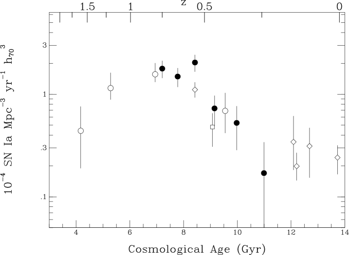
Figure 7: Rates from the IfA Deep Survey (large filled circles) as a function of cosmological time, compared with previously published results: Tonry et al. 2003 (open square); Dahlen et al. 2004 (open circles); open diamonds represent, with increasing redshift, Cappellaro et al. (1999), Madgwick et al. (2003), Blanc et al. (2000), Hardin et al. (2000), and Pain et al. (2002). Note the large discrepancy between the IfA Deep Survey measurement and that of Pain et al. at $z=0.55$. This may indicate sample contamination of this redshift bin.

In Figure  7 we plot these results, as well as recent values from the literature for comparison. The large number of SNIa discovered during the IfA Deep Survey enables us to examine the Type Ia SNR as a function of redshift to an unprecedented level of detail. The rates calculated at $z=0.35$ and $z=0.45$ are in good agreement with the recent calculations presented in the literature, indicating that our sample selection and calculation procedure appear to be working properly. Similarly, the derived value at $z=0.75$ agrees well with that at $z=0.80$ given by Dahlen et al. (2004), confirming their observation of a significantly higher rate at $z\approx 0.8$ compared to $z\approx 0.45$. Our observed point at $z=0.65$ also appears to describe a fairly gradual increase in the SNR as a function of redshift, peaking at perhaps $z\approx 0.8-1.0$, with the points between $z=0.65-0.80$ consistent with a flattening in the rate over this redshift range.

The point at $z=0.55$ is somewhat of an outlier to such a picture. Rather than displaying the general trend of gradually increasing SNR to higher redshifts, the rate at $z=0.55$ is sharply higher than that at $z=0.45$, and higher than the rate measured for $any$ higher redshift bin. It is also substantially higher than the value reported by Pain et al. (2002) at the same redshift, with which it is discrepant at $>3\sigma$ level. We have investigated several systematic effects that could potentially cause this point to be biased to such a high value. First, the redshift-independent BATM method that we have used may tend to incorrectly measure distances for our sample SN, scattering objects into this bin. Among objections to this theory are the good agreement the higher-$z$ and lower-$z$ bins exhibit with previously published rate measurements and the large size of the discrepancy. If there were a large number of SNIa being improperly placed into the $z=0.55$ bin, it seems likely that moving them into their proper bins would create a discrepancy in these other bins where none currently exists. We have also checked the derived redshifts for the 23 known SNIa from Barris et al. (2004), and no spike at $z=0.55$ is observed, a reassuring sign that the $z$-free BATM distances are not systematically overpopulating the bin with SN Ia from other bins. Another possibility is that there are non-SNIa in the sample which tend to be fit at distances corresponding to $z\approx 0.5$. The most obvious candidates for interlopers are CC SN (either Type Ib/c or Type II), though AGN and flaring variable stars could also perhaps mimic SNIa light-curves in certain cases. SN II have a very broad (and uncertain) luminosity function (Richardson et al. 2002), but are roughly two magnitudes fainter than SNIa. We do not believe that SN II are plausible contaminants, however, because their light-curve shapes are quite different from those of SNIa, which will cause most SN II to be rejected by our goodness-of-fit tests, or even be rejected during the LCOE analysis (as for the 2 SN II that we know of that are not included even in our sample of 133). SN Ib/c have light-curve shapes similar to Type Ia, and also have a much fainter luminosity function, so it is possible that they could fool our fitting procedure. To test this, we have measured $z$-free distances for SN 1994I, a typical SN Ic with significant extinction. The light-curves do tend to be fit at higher redshifts, but for this particular SN are not placed in the $z=0.55$ bin. The most important revelation is that the derived fit colors are extremely blue. Such objects would not be able to contaminate our sample, because we would reject it based on such unusual colors. We therefore do not have an obvious source for contamination in the $z=0.55$ bin, and conclude that the rate measurement at this redshift is accurate. We also expect that the analysis that we have performed for this bin gives a general sense of the potential systematic effects on any individual bin, which we also do not expect to be severe.

There is strong justification for the expectation that the systematic errors are small, certainly in comparison with the statistical errors. The primary sources arise from the possibility that the assumptions that were made in Section  4 are incorrect. The most obvious potential discrepancies include the evolution of the assumed dust extinction model, which is tied to an assumed distribution of SN Ia in different types of host galaxy, and the uniformity of the spectrophotometric templates that we have used, which affects both the maximum brightness and the calculations K-corrections. However, the well-established properties of SN Ia are such that effects such as these should be small. Their high degree of heterogeneity implies that our templates should be sufficient for an accurate rate calculation. As has been shown by Dahlen et al. (2004) and others, the value of dust extinction typically needs to be increased by a factor of several before its effects are comparable with statistical errors for similar SN rate calculations.

The primary concern that we have about the accuracy of our rate measurements is for incompleteness at high redshifts. It is clear that our redshift bins at $z>0.75$ are highly incomplete. Attempting to fully quantify the potential systematic errors that may afflict the lower-$z$ bins, e.g. through detailed Monte Carlo simulations of the effects of slight variations in dust extinction, will have much less impact on the conclusions that may be drawn from the measured SN rates than will the recognition that the highest-$z$ bins are incomplete to such an extent that the measurements should be disregarded. As we show in the next section, we believe that the conclusions drawn by Strolger et al. (2004) may be entirely driven by measurements that are highly incomplete rather than reflecting actual evolution in the Type Ia SNR.

6 Comparison with Star Formation Models

The SNR measurements shown in Figure  7 are in general described by a gradual increase in the Type Ia SNR with higher redshift, with signs of flattening by $z\approx 0.8$, perhaps even as early as $z\approx 0.6$. The calculations from the IfA Deep Survey agree well with the recent results from Tonry et al. (2003) and Dahlen et al. (2004), and confirm the indication from the latter that there is a substantial increase in the SNR between $z\approx 0.45$ and $z\approx 0.8$. The size of our sample enables us to trace the history of the SNR in more detail than previously possible. We would like to compare the observed SNR to measurements of the SFR in order to determine whether insight can be gleaned into potential progenitor pathways.

We can first quantify the relationship between SFR and the Type Ia SNR. We have chosen to use the SFR values of Steidel et al. 1999 in order to facilitate a comparison with the recent results presented by Strolger et al. (2004). As shown by the recent compilation of Hopkins et al. (2004), measurements of cosmological SFR at different wavelengths are so widely discrepant that it is not at all clear how well the Steidel et al. values reflect the actual underlying star formation. However, Strolger et al. (2004) recently used the Steidel et al. values to draw profound conclusions about the relationship between SFR and SNR, so we have chosen to do so also in order to facilitate a comparison with their results. We use all SNR measurements at $z<1$ from the surveys mentioned previously. We do not use the higher $z$ values from Dahlen et al. (2004) for two reasons–first, neither the IfA Deep Survey nor any other survey has measured SNR at such high redshifts, so there is no confirmation of the apparent turnover in the SNR indicated by these values. Second, the results of Strolger et al. (2004) indicating a long delay time between SFR and SNR are strongly driven by the measurements at high $z$, so much so that the addition of our measurements at $z<0.8$ will not change their conclusions. We wish to test whether there is any evidence for the Strolger et al. conclusions other than the two highest $z$ redshift bins measured by Dahlen et al.

Using these two collections of SNR and SFR values, we fit over a range of delay times for the SFR/SNR ratio that best matches the observations, using a least-squares analysis. We interpolate the SFR measurements in order to compare with the SNR, rather than choosing a parameterization such as that defined by Giavalisco et al. (2004). We have chosen to do so because it is not clear that this parameterization accurately reflects the published SFR measurements. For example, the SFR measurements of Steidel et al. (1999) are constant between $z=0.75-1.76$ ($t\approx 4-7$ Gyr), yet the model indicates an increase of nearly a factor of 3 over this range. Considering the large observational uncertainties (and the cosmic variance which may afflict the SFR measurements), it is not clear that the model of Giavalisco et al. (2004) should be preferred over other models, including one produced directly from the observations, for comparing with the Type Ia SNR.

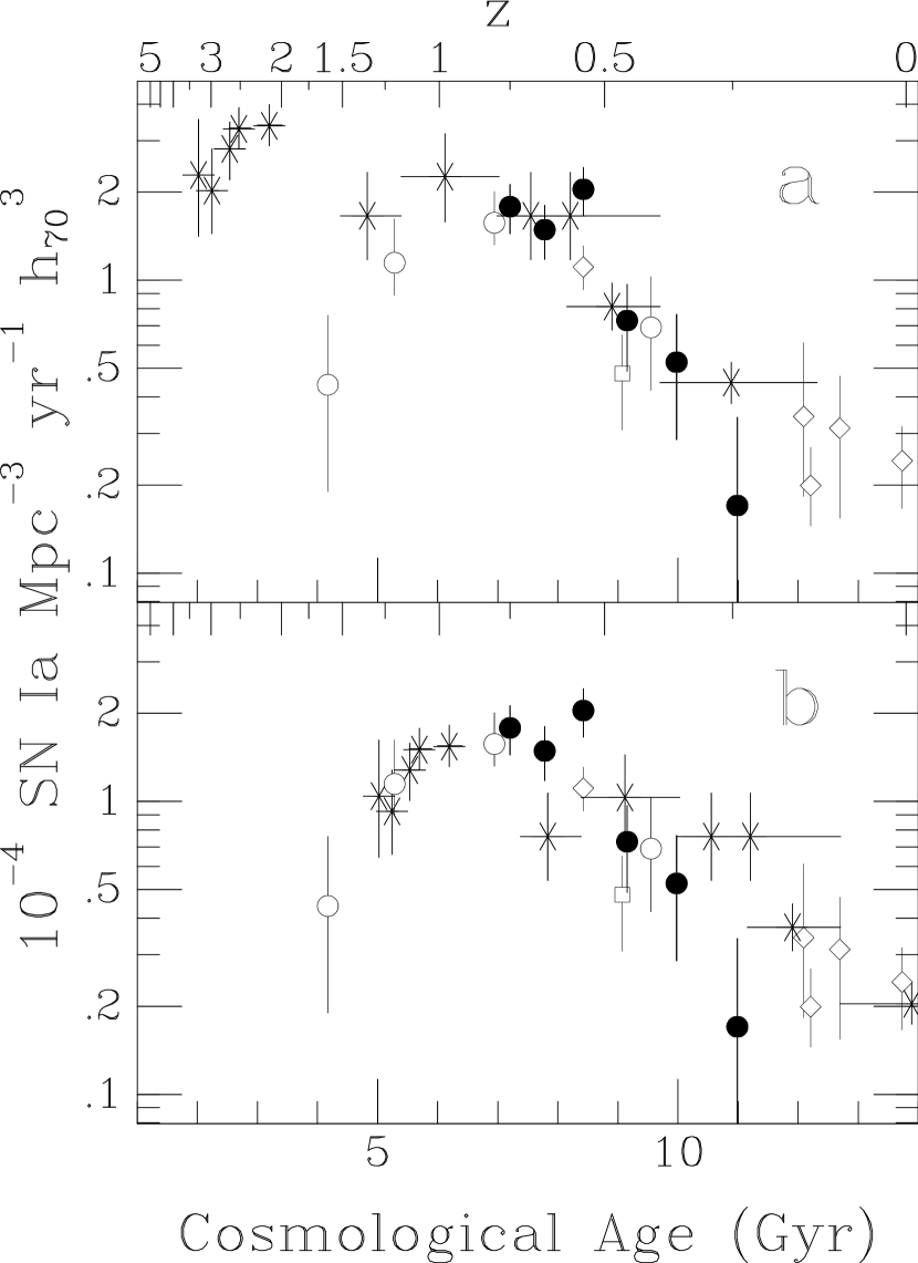
Figure 9: As in Figure  7, Type Ia SNR calculations from the IfA Deep Survey (large filled circles), and previously published rates as given in Figure  7. Also included in this figure are SFR measurements from Steidel et al. 1999 (asterisks, scaled to overlie the SNR values). a) A simple linear shift of $t=1$ Gyr is introduced to the SFR observations as indicated by Table  2. Note the common plateau feature between $t\approx 5-8$ Gyr, as well as the subsequent decline seen in both SFR and SNR measurements. b) A time-delay of $t=4$ Gyr is introduced to the SFR observations as suggested by Strolger et al. (2004). This match is produced by aligning the apparent turnover in the SNR beginning at $z\approx 1.2$ with SFR measurements at $z\approx 3-6$. However, note the poor match between the actual SFR and SNR observations between $t\approx 8-12$ Gyr ($z\approx 0.75-0.25$) in comparison to the linear shift of $t\approx 1$ Gyr shown in a).

The best agreement between SFR and SNR measurements occurs at $t\approx 1$ Gyr, with a derived ratio of SFR/SNR = 580 $h_{70}^{-2}$ M${}_{\mathord{\odot}}$/SNIa (see Table  2 and Figure  8; it should be noted that the deviation of the calculated $\chi^{2}/N$ from 1 is solely due to the $z=0.55$ bin). In Figure  9a we compare the SNR and SFR measurements, shifting the latter by $t=1$ Gyr. This time delay reflect the best-fit value from Table  2, and Figure  9a demonstrates that it matches features evident in both observations—a sudden drop at $z\approx 0.55$ ($t\approx 8.4$ Gyr) in the SNR measurements, after previously being relatively constant for a long period of time ($t\approx 3$ Gyr or more). While we have discussed the possibility of sample contamination afflicting our SNR measurement at $z\approx 0.55$, it may indeed be a sign of a short ($t\approx 1$ Gyr) delayed reaction to a similar relatively abrupt change in the star formation rate, with the repeated caveat that such features in the SFR are even more uncertain than for the SNR.

In Figure  9b we plot the SFR and SNR observations, with a long delay time of $t=4$ Gyr. This value is the best-fit model given by Strolger et al. (2004) for the ACS data and previously published SNR measurements, determined through a comparison with the Giavalisco et al. (2004) SFR model. It is obvious that the apparent turnover indicated by the point at $z=1.6$ is the driving force behind the findings by Dahlen et al. (2004) and Strolger et al. (2004) of a long time-delay between the SFR and SNR. An examination of Figure  9 reveals that the more detailed redshift coverage provided by the large IfA Deep Survey sample does not agree as well with this model as for a short delay time. As discussed above, the flattening in the SNR (indicated by measurements from both the IfA Deep and ACS Higher-Z Surveys) between $z=0.5-1.2$ is well matched by a similar plateau in the SFR $t\approx 1$ Gyr earlier. In Figure  9b, however, the constant region in the SFR measurements has been shifted to correspond to redshifts between $z=0.25-0.7$, a region during which the SNR declines substantially. This reveals the reason for the significantly worse fits with increasing time delay values given in Table  2 and shown in Figure  8—the slope indicated by the SFR measurements is simply too shallow in comparison with SNR values at times $t>2$ Gyr later (though the match with the local SNR measurement of Cappellaro et al. 1999 is somewhat at odds with this finding). While the Giavalisco et al. (2004) model curve utilized by Strolger et al. (2004) fits the data reasonably well, especially when constrained by the $z=1.6$ ACS measurement, the match between the actual SFR and SNR observations is poor.

6.1 WD Progenitor Efficiency

We can also compare the values of SFR/SNR to the expected number of white dwarfs produced during star formation. We adopt a Salpeter (1955) initial mass function (IMF) with a slope of $m=-2.35$ and a mass range of $0.1-125$ M${}_{\mathord{\odot}}$. As noted in Section  1.1, C-O WDs are produced by stars with a main-sequence mass of $3-8$ M${}_{\mathord{\odot}}$ (Nomoto et al. 1994). We can therefore integrate over the IMF to calculate the number of such white dwarfs that are produced per unit star formation:

$$N(C-O\ WD)=\int_{3M_{\mathord{\odot}}}^{8M_{\mathord{\odot}}}\psi(M)dM\ /\int_{0.1M_{\mathord{\odot}}}^{125M_{\mathord{\odot}}}M\psi(M)dM,$$

which results in a value of N(C-O WD)=0.021 M${}_{\mathord{\odot}}^{-1}$. Table  2 includes values for the number of C-O white dwarfs formed by the amount of star formation indicated by the SFR/SNR ratio. For time delays $t=0-1$ Gyr, there are $\approx 10-12$ C-O WDs for each SNIa (adopting $h=0.7$), which indicates an efficiency of 8–10% ($\pm$4%) for producing SNIa (see Figure  8). This value is somewhat higher than the 5–7 % determined by Dahlen et al. (2004), though within the uncertainties.

The various models for SNIa explosion mechanisms discussed in Section  1.1 can in general all accommodate the delay time of $t\approx 1$ Gyr derived here. In fact, even the long delay time of $t=3-4$ Gyr preferred by Strolger et al. (2004) cannot strongly rule out most progenitor pathways, due to theoretical uncertainties. A substantial amount of work must be done to further investigate this matter. The measurements presented here should guide the work of theorists and modelers into providing further constraints.

6.2 Predicting the Type Ia SNR at $z>1$

Based on the above SFR/SNR ratios, we can predict the SNR that we expect at higher redshifts assuming that SNIa do indeed follow the SFR after a delay of $t\approx 1$ Gyr. At $z=1.76$ $(t\approx 3.8$ Gyr), the SFR is 0.09${}_{-0.03}^{+0.04}$ M${}_{\mathord{\odot}}$ Mpc^-3 yr^-1 $h_{70}$. Shifting this point by $t=1$ Gyr would place it at approximately $z=1.35$. If we adopt SFR/SNR = 580$\pm$240 $h_{70}^{-2}$ M${}_{\mathord{\odot}}$/SNIa (for a $t=1$ Gyr time delay), we obtain a predicted Type Ia SNR of 1.5$\pm$0.8 x 10^-4 SNIa Mpc^-3 yr^-1 $h_{70}^{3}$, in good agreement with the value of 1.15${}_{-0.26}^{+0.47}$ x 10^-4 SNIa Mpc^-3 yr^-1 $h_{70}^{3}$ measured by Dahlen et al. (2004).

The next measurement of the SFR at higher redshift is at $z\approx 3$ ($t\approx 2.2$ Gyr), which corresponds to $z\approx 2$ after a shift of $t=1$ Gyr. This measurement of 0.18${}_{-0.03}^{+0.03}$ M${}_{\mathord{\odot}}$ Mpc^-3 yr^-1 $h_{70}$ would predict a Type Ia SNR of 3.0$\pm$1.3 x 10^-4 SNIa Mpc^-3 yr^-1 $h_{70}^{3}$ using SFR/SNR = 580$\pm$240 $h_{70}^{-2}$ M${}_{\mathord{\odot}}$/SNIa. This strongly conflicts with the trend suggested by the $z=1.6$ ACS SNR measurement of 0.44 x 10^-4 SNIa Mpc^-3 yr^-1 $h_{70}^{3}$. However, it agrees well with the predicted range of 1-3.5 x 10^-4 SNIa Mpc^-3 yr^-1 $h_{70}^{3}$ given by Scannapieco & Bildsten 2005 (astro-ph/0507456).

Further measurements of the SNR at $z>1$ must be performed in order to confirm the apparent plateau and decline indicated by the ACS GOODS Survey. We note that since it was a continuous survey, an analysis similar to the LCOE process described here can be carried out on the survey observations. This would be helpful to overcome the difficulties inherent in constructing a complete sample under the time constraints of SN surveys (recall the discussion in the introduction), and ensure the accuracy of their high-$z$ SNR measurements. Without clear evidence for a turnover, there is little power to differentiate between a shift in amplitude and a shift in time, so both short ($t\lesssim 1$ Gyr) and long ($t\approx 3-4$ Gyr) time delays can be accommodated. Confirmation of a turnover would be a strong indication of the need for a long ($t\approx 3-4$ Gyr) time delay between SFR and SNR (see Strolger et al. 2004). Using the actual SFR measurements rather than the parametrized model of Giavalisco et al. (2004) produces a substantially better match to the SNR measurements for short delay times. More measurements at $z>0.8$ are necessary before the behavior of the SNR can be determined at these redshifts. At present, the observations are consistent with a fairly short ($t\approx 1$ Gyr) time delay.

7 Conclusion

The IfA Deep Survey, with its continuous observations of large areas of sky, provides a unique opportunity for a general exploration of the astronomical time domain at very faint magnitude limits and over a wide range of timescales. We have analyzed the survey images with software designed to detect all variable objects and extract a complete sample of SNIa, constructing tests which efficiently detect variable objects with SN-like light-curves. From an initial number of variable objects of a few tens of thousands per field, complete to $m_{I}\approx 24.1$, a sample of approximately 700 candidates was selected based upon these tests, reduced to 133 SN candidates upon visual inspection, nearly 100 of which were determined to be useful for cosmological analysis. The thorough LCOE analysis process we have implemented has allowed us to collect an extremely large, complete SN sample extending to $z\approx 0.8$.

We have investigated the rates of SNIa indicated by the complete sample obtained from the IfA Deep Survey. The large size and broad redshift range of our sample makes it uniquely powerful for probing the SNR throughout cosmological history. We find good agreement between our calculated rates and those previously reported at $z\approx 0.45$ and $z\approx 0.8$, confirming the recent findings of Dahlen et al. (2004) that the SNR rises substantially during this period of cosmological history.

Through a comparison with measurements of the SFR over a wide range of redshifts, we observe no evidence for a significant delay between the SFR and the Type Ia SNR. The best-fit values are for a time-delay of $t\approx 1$ Gyr, in contrast to the much longer values of $t=3-4$ Gyr suggested recently based on results from the ACS GOODS SN survey (Dahlen et al. 2004, Strolger et al. 2004). This short value is supported by metallicity observations in the solar neighborhood as well as in high-$z$ damped Ly-$\alpha$ systems. We are unable to conclusively determine a preferred progenitor system, since most theoretical models can accommodate a delay of $t\approx 1$ Gyr between the SFR and Type Ia SNR.

We derive a best-fit value of SFR/SNR $\approx 580\ h_{70}^{-2}$ M${}_{\mathord{\odot}}$/SNIa for the conversion factor between star formation and SN rates, as determined for a delay time of $t\approx 1$ Gyr between the SFR and the Type Ia SNR. With this value we predict a SNR value at $z\approx 1.25$ in agreement with the published results of Dahlen et al. (2004), but at $z\approx 2$ predict a significantly higher value than they have reported at $z=1.6$. Further investigation into the rates at these high redshifts is required before additional constraints may be placed on the relationship between SFR and SNR, which is necessary to place limits on possible progenitor pathways. A confirmation of the plateau and decline of the Type Ia SNR at $z>1$ would indicate a substantial ($t\approx 3-4$ Gyr) delay time. Current measurements at $z\approx 1$ and below are not capable of conclusively determining the delay times, and are consistent with a short ($t\lesssim 1$ Gyr) time delay with respect to the SFR.

Table 1: IfA Deep Survey Supernova Rates

$z$	N	N	Npredict	Rate	$\sigma$(Rate)
0.25	9	1	5.9	0.17	0.17
0.35	9	5	9.5	0.53	0.24
0.45	15	9	12.3	0.73	0.24
0.55	40	29	14.2	2.04	0.38
0.65	25	23	15.4	1.49	0.31
0.75	32	28	15.7	1.78	0.34

Table 2: SFR/SNR Ratios

$t$(Gyr)	$\chi^{2}/N$	SFR/SNR($\sigma$)	N(WD)($\sigma$)	SN/WD($\sigma$)
0.0	3.7	450(200)	9.5(4.2)	0.11(0.05)
0.5	3.4	520(240)	10.9(5.0)	0.09(0.04)
1.0	2.2	580(280)	12.2(5.9)	0.08(0.04)
1.5	2.8	690(310)	14.5(6.5)	0.07(0.03)
2.0	5.5	905(380)	19.0(8.0)	0.05(0.02)
2.5	5.4	970(590)	20.4(12.4)	0.05(0.03)
3.0	6.6	1060(770)	22.3(16.2)	0.04(0.03)
3.5	8.4	1170(820)	24.6(17.2)	0.04(0.03)
4.0	10.3	1380(910)	29.0(19.1)	0.03(0.02)
4.5	9.6	1430(1000)	30.0(21.0)	0.03(0.02)

Figure 1: Light-curve of example prototype object classified as AGN-like.

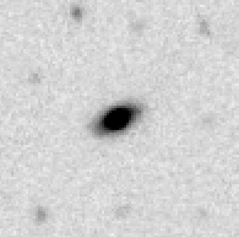
Figure 2: Image of prototype object classified as AGN-like (light curve given in Figure  1).

Figure 3: Light-curve of example prototype object classified as Variable-star-like.

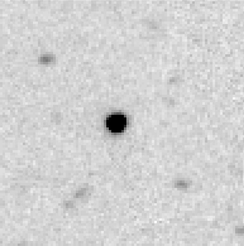
Figure 4: Image of prototype object classified as Variable-star-like (light curve given in Figure  3).

Figure 5: Histogram of the fraction of SN from each bin that were rejected during the culling process from 133 to 98 SN. Note the decline in the rejected fraction to high-$z$, which we attribute to the fainter luminosity function of the most likely potential contaminants (primarily CC SN).

Figure 6: Histogram of the number of discovered SN as a function of redshift. Also shown is the envelope expected to describe the histogram (with arbitrary normalization) were it merely a reflection of the changing volume and redshift being sampled. The steep rise of the histogram with increasing redshift indicates that the numbers of discovered objects are indeed a sign of an actual increase in the SNR.

Figure 8: Trends in $\chi^{2}/N$ (filled circles) and C-O WD explosion efficiency (open circles) as a function of delay-time. Note the best-fit values for a match between SFR and SNR measurements occurs at a time delay of $t\approx 1$ Gyr. Longer time delays produce substantially poorer fits.

References

- Barris (2004) Barris, B.J. 2004, Ph.D. Thesis, University of Hawaii
- Barris & Tonry (2004) Barris, B.J., & Tonry, J.L. 2004, ApJ, 613, L21
- Barris et al. (2004) Barris, B.J., et al. 2004, ApJ, 602, 571
- Becker et al. (2004) Becker, A., et al. 2004, ApJ, 611, 418
- Blanc et al. (2004) Blanc, G., et al. 2004, A&A, 423, 881
- Cappellaro et al. (1999) Cappellaro, E., Evans, R., & Turatto, M. 1999, A&A, 351, 459
- Cassisi et al. (1998) Cassisi, S., Iben, I.J., & Tornambe, A. 1998, ApJ, 496, 376
- Cuillandre et al. (1999) Cuillandre, J-C., et al. 1999, CFH Bulletin. 40
- Dahlen et al. (2004) Dahlen, T., et al. 2004, ApJ, 613, 189
- Filippenko (1997) Filippenko, A.V. 1997, ARA&A, 35, 309
- Filippenko et al. (1992) Filippenko, A.V., et al. 1992, AJ, 104, 1543
- Gal-Yam & Maoz (2004) Gal-Yam, A., & Maoz, D. 2004, MNRAS, 347, 942
- Giavalisco et al. (2004) Giavalisco, M., et al. 2004, ApJ, 600, L103
- Hardin et al. (2000) Hardin, D., et al. 2000, A%A, 362, 419
- Hatano et al. (1998) Hatano, K., Branch, D., & Deaton, J. 1998, ApJ, 502, 177
- Hillebrandt & Niemeyer (2000) Hillebrandt, W., & Niemeyer, J.C. 2000, ARA&A, 38, 191
- Hopkins (2004) Hopkins, A.M. 2004, ApJ, 615, 209
- Iben & Tutukov (1984) Iben, I., & Tutukov, A.V. 1984, ApJS, 54, 335
- Knop et al. (2003) Knop, R.A., et al. 2003, ApJ, 598, 102
- Kobayashi et al. (1998) Kobayashi, C., et al. 1998, ApJ, 503, L155
- Kobayashi et al. (2000) Kobayashi, C., Tsujimoto, T., & Nomoto, K. 2000, ApJ, 539, 26
- Koester et al. (2001) Koester, D., et al. 2001, A&A, 378, 556
- Li et al. (2001) Li, W., et al. 2001, ApJ, 546, 734
- Livio (2000) Livio, M. 2000, in Type Ia Supernovae, Theory and Cosmology. Edited by J.C. Niemeyer and J.W. Truran. Published by Cambridge University press, 33
- Livio & Riess (2003) Livio, M., & Riess, A.G. 2003, ApJ, 594, 93L
- (26) Madau, P., della Valle, M., & Panagia, N. 1998, MNRAS, 297, L17
- Madgwick et al. (2003) Madgwick, D.S., et al. 2003, ApJ, 599, L33
- Matteucci & Greggio (1986) Matteucci, F., & Greggio, L. 1986, A&A, 154, 279
- Matteucci & Recchi (2001) Matteucci, F., & Recchi, S. 2001, ApJ, 558, 351
- Miyazaki et al. (1998) Miyazaki, S. et al. 1998, in Proc. SPIE, 3355, 363
- (31) Nomoto, K. 1982a, ApJ, 257, 780
- (32) Nomoto, K. 1982b, ApJ, 253, 798
- Nomoto et al. (2000) Nomoto, K., et al. 2000, in Type Ia Supernovae, Theory and Cosmology. Edited by J.C. Niemeyer and J.W. Truran. Published by Cambridge University press, 63
- Nomoto et al. (1994) Nomoto, K., et al. 1994, in Proc. Les Houches Session LIV, Supernovae, ed. S.A. Bludman, R. Mochkovitch, & J. Zinn-Justin (Amsterdam: Elsevier Sci. Pub), 199
- Pain et al. (2002) Pain, R., et al. 2002, ApJ, 577, 120
- Pain et al. (1996) Pain, R., et al. 1996, ApJ, 473, 356
- Perlmutter et al. (1995) Perlmutter, S., et al. 1995, in Thermonuclear Supernovae, ed. P. Ruiz-Lapuente, R. Canal, & J. Isern (NATO ASI Ser. C, 486) (Dordrecht: Kluwer), 74
- Perlmutter et al. (1997) Perlmutter, S., et al. 1997, ApJ, 483, 565
- Perlmutter et al. (1999) Perlmutter, S., et al. 1999, ApJ, 517, 565
- Pettini et al. (1999) Pettini, M., et al. 1999, ApJ, 510, 576
- Richardson et al. (2002) Richardson, D., et al. 2002, AJ, 123, 745
- Riess (2002) Riess, A.G. 2002, BAAS, 34, 1161
- RPK (96) Riess, A.G., Press, W.H., & Kirshner, R.P. 1996, ApJ, 473, 88
- Riess et al. (1998) Riess, A.G., et al. 1998, AJ, 116, 1009
- Riess et al. (2004) Riess, A.G., et al. 2004, ApJ, 600, L163
- Ruiz-Lapuente et al. (2004) Ruiz-Lapuents, P., et al. 2004, Nature, 431, 1069
- Ruiz-Lapuente et al. (2000) Ruiz-Lapuente, P., et al. 2000, in Type Ia Supernovae, Theory and Cosmology. Edited by J.C. Niemeyer and J.W. Truran. Published by Cambridge University press, 49
- Ruiz-Lapuente et al. (1995) Ruiz-Lapuente, P., Burkert, A., & Canal, R. 1995, ApJ, 447, L69
- Saffer et al. (1998) Saffer, R.A., Livio, M., & Yungelson, L.R. 1998, ApJ, 502, 394
- Salpeter (1955) Salpeter, E.E. 1955, ApJ, 121, 161
- Schmidt et al. (1998) Schmidt, B.P., et al. 1998, ApJ, 507, 46
- Steidel et al. (1999) Steidel, C.C., et al. 1999, ApJ, 519, 1
- Strolger et al. (2004) Strolger, L.-G., et al. 2004, ApJ, 613, 200
- Tonry et al. (2003) Tonry, J.L., et al. 2003, ApJ, 594, 1
- Vinko et al. (2001) Vinkó, J., et al. 2001, AJ, 121, 3127
- Webbink (1984) Webbink, R.F. 1984, ApJ, 277, 355
- Yungelson & Livio (2000) Yungelson, L.R., & Livio, M. 2000, ApJ, 528, 108