Optical Lightcurve & Cooling Break of GRB 050502A

Abstract

We present lightcurves of the afterglow of GRB 050502A, including very early data at $t-t_{GRB}<60$ s. The lightcurve is composed of unfiltered ROTSE-IIIb optical observations from 44 s to 6 h post-burst, $R$-band MDM observations from 1.6 to 8.4 h post-burst, and PAIRITEL $JHK_{s}$ observations from 0.6 to 2.6 h post-burst. The optical lightcurve is fit by a broken power law, where $t^{\alpha}$ steepens from $\alpha=-1.13\pm 0.02$ to $\alpha=-1.44\pm 0.02$ at $\sim$5700 s. This steepening is consistent with the evolution expected for the passage of the cooling frequency $\nu_{c}$ through the optical band. Even in our earliest observation at 44 s post-burst, there is no evidence that the optical flux is brighter than a backward extrapolation of the later power law would suggest. The observed decay indices and spectral index are consistent with either an ISM or a Wind fireball model, but slightly favor the ISM interpretation. The expected spectral index in the ISM interpretation is consistent within $1\sigma$ with the observed spectral index $\beta=-0.8\pm 0.1$; the Wind interpretation would imply a slightly ($\sim 2\sigma$) shallower spectral index than observed. A small amount of dust extinction at the source redshift could steepen an intrinsic spectrum sufficiently to account for the observed value of $\beta$. In this picture, the early optical decay, with the peak at or below $4.7\times 10^{14}$ Hz at 44 s, requires very small electron and magnetic energy partitions from the fireball.

1 Introduction

GRB afterglows are typically observed to decay as power laws in time (as reviewed by, e.g., Piran, 2005). The leading afterglow model is the synchrotron fireball (Mészáros & Rees, 1997; Sari et al., 1998). It describes the afterglow as synchrotron emission from shock-accelerated electrons with a broken power law spectral energy distribution, with several characteristic break frequencies. When the typical synchrotron frequency ($\nu_{m}$) or the cooling frequency ($\nu_{c}$) passes through the optical bands, the model predicts a break in the lightcurve.

The fireball model’s spectral breaks have different power law indices depending upon the circumburst medium (as discussed by Mészáros et al., 1998). The different resulting lightcurves allow important physical distinctions to be inferred from early afterglow observations. One example is the anticipated difference between a constant circumburst density (called “ISM”) or $r^{-2}$ density gradient (called “Wind” as it resembles the environment produced by a steady mass-loss wind outflow). The GRB follow-up community has worked to produce ever-earlier observations in order to detect lightcurve breaks.

The passage of the cooling frequency, $\nu_{c}$, has been inferred from changes in the broadband spectral index. The first such example was GRB 970508 (Galama et al., 1998), where the optical-to-X-ray slope steepened as if $\nu_{c}$ were passing between them. Direct evidence of a cooling break passage in lightcurves is rarer. GRB 030329 showed a shallow change of slope at $t<0.25$ d postulated to be the cooling break (Sato et al., 2003), although the standard fireball picture is complicated in that case, possibly with “layered” ejecta giving 2 jets and 2 jet breaks (Berger et al., 2003). More recently, Huang et al. (2005) found a shallow break in the GRB 040924 afterglow better explained by $\nu_{c}$ than a jet break.

Here we report observations of the GRB 050502A afterglow in unfiltered optical and $RJHK_{s}$ bands. The optical data span nearly 3 logarithmic decades in time and begin at $t<1$ min after the start of the GRB. We discuss the lightcurves in the context of the fireball model.

2 Observations

This paper’s optical and near-IR lightcurves are the result of three observation teams with different instruments at separate sites: ROTSE-III, PAIRITEL, and MDM.

The ROTSE-III array is a worldwide network of 0.45 m robotic, automated telescopes, built for fast ($\sim 6$ s) responses to GRB triggers from satellites such as HETE-2 and Swift. They have a wide ($1\fdg 85\times 1\fdg 85$) field of view imaged onto a Marconi $2048\times 2048$ back-illuminated thinned CCD, and operate without filters, with a bandpass from approximately 400 to 900 nm. ROTSE-IIIb is located at McDonald Observatory in Texas. The ROTSE-III systems are described in detail in Akerlof et al. (2003).

The 1.3m diameter PAIRITEL (Peters Automated Infrared Imaging Telescope) is a fully automated incarnation of the system used for the Two Micron All-Sky Survey (2MASS). It is located on the Ridge at Mt. Hopkins, Arizona. The camera consists of three 256$\times$256 NICMOS3 arrays that image simultaneously the same $8.\!^{\prime}5\times 8.\!^{\prime}5$ portion of the sky at $J$, $H$, and $K_{s}$ bands (central wavelengths 1.2, 1.6, and 2.2 $\mu$m).

The MDM Observatory is located at Kitt Peak, Arizona. It includes the 1.3m McGraw-Hill telescope, which covers an $8.\!^{\prime}7\times 8.\!^{\prime}7$ field of view. This instrument operates with a standard set of filters. The camera is a SITe $1024\times 1024$ thinned, backside illuminated CCD, with a pixel scale of $0.\!^{\prime\prime}508$.

On 2005 May 2, INTEGRAL detected GRB 050502A (INTEGRAL trigger 2484) at 02:13:57 UT. The position was distributed as a Gamma-ray burst Coordinates Network (GCN) notice at 02:14:36 UT, with a $3\arcmin$ radius error box, 39 s after the start of the burst (Gotz et al., 2005). The burst had a duration of 21 s, with a fluence of $1.4\times 10^{-6}\,\mathrm{erg}\,\mathrm{cm}^{-2}$ in the 20-200 keV band (Gotz & Mereghetti, 2005).

ROTSE-IIIb responded automatically to the GCN notice in 5.0 s with the first exposure starting at 02:14:41.0 UT, 44 s after the burst and only 23 s after the cessation of $\gamma$-ray activity. The automated scheduler began a program of ten 5-s exposures, ten 20-s exposures, and 412 60-s exposures. The first exposure was taken during evening twilight hours, and ROTSE-IIIb was able to follow the burst position until the morning twilight. The early images were affected by scattered clouds and a bright sky background. Near real-time analysis of the ROTSE-III images detected a $14^{th}$ magnitude fading source at $\alpha=13^{h}29^{m}46\fs 3$, $\delta=+42\arcdeg 40\arcmin 27\farcs 7$ (J2000.0) that was not visible on the Digitized Sky Survey red plates, which we reported via the GCN Circular e-mail exploder within 40 minutes of the burst (Yost et al., 2005).

The PAIRITEL instrument on Mt. Hopkins received the GRB 050502A trigger before dusk and generated a rapid response ToO. When an interrupt is generated by a new burst at nighttime, a new set of observations is queued, overriding all other targets. Typical time from GCN alert to slew is 10 seconds and typical slew times are 1-2 minutes. Since this burst occurred before nighttime science operations, it overrode the scheduled observations related to telescope pointing. This behavior yielded a bad pointing model in the first set of observations and has subsequently been prohibited. The first set of usable imaging began at 02:52:39.5 UT, or approximately 39 minutes after the trigger. Several imaging epochs were conducted over the following 5 hours.

PAIRITEL images were acquired with double-correlated sampling with effective exposure times of 7.848 seconds and dithered over several positions during a single epoch of observation. Typical total integration times are between 2 to 30 minutes with approximately 10–30 different dither positions.

The MDM Observatory began $R$-band observations 1.8 hours after the burst, following the initial ROTSE GCN report. 21 exposures were taken of the GRB field spanning a total of 6.4 hours.

3 Data Reductions

The three diverse datasets required different photometric reductions. All the data described below are given in Table 1.

The ROTSE-IIIb images were dark-subtracted and flat-fielded with its standard pipeline. The flat-field was generated from 30 twilight images. SExtractor (Bertin & Arnouts, 1996) was applied for the initial object detection. The images were then processed with a customized version of the DAOPHOT PSF fitting package (Stetson, 1987) that has been ported to the IDL Astronomy User’s Library (Landsman, 1995). The PSF is calculated for each image from a set of $\sim 50$ well-measured stars within $12^{\prime}$ of the target location. The PSF is fit simultaneously to groups of stars using the nstar procedure (Stetson, 1987). Relative photometry was then performed using 13 neighboring stars.

ROTSE-III magnitudes are calibrated as $R$-equivalent to accomodate ROTSE’s peak optical bandpass sensitivity at red wavelengths. The $R$-equivalent magnitude zero-point is calculated from the median offset to the USNO 1 m $R$-band standard stars (Henden, 2005) in the magnitude range of $13.5<V<20.0$ with the color of typical stars in the field such that $0.4<V-R<1.0$. As we have no data on afterglow color information at the early time, no additional color corrections have been applied to the unfiltered data, and the magnitudes quoted are then treated as $R$-band and referred to as “$C_{R}$”.

The PAIRITEL data were processed through its custom reductions pipeline and then combined into mosaics as a function of epoch and filter. The mosaicking used a cross-correlation between reduced images to find the pixel offsets for the dithers. Final images were constructed using a static bad pixel mask and drizzling (Fruchter & Hook, 1997). Bias and sky frames are obtained for each frame by median combining several images before and after that frame. Flat fields are applied from archival sky flats, and are known to be highly stable over long periods of time. Aperture photometry was performed in a 3.5 pixel radius aperture (the average seeing FWHM was 2.4 pixels). The PAIRITEL photometric zeropoints for each of $J$, $H$, and $K_{s}$ were determined from 2MASS catalog stars, of which there are $\sim 20$ in the field.

The MDM data were processed using standard IRAF/DAOPHOT procedures. Aperture photometry was performed in a $1.5\!^{\prime\prime}$ radius aperture (average seeing was $\sim$ $1.5\!^{\prime\prime}$) centered on the OT and nearby field stars. Instrumental magnitudes were then transformed to the $R$ system using the latest calibration provided by Henden et al. (2005), using differential photometry for each image with respect to two Henden stars, the only ones available in the MDM field (RA, DEC = 13:30:04.3, +42:41:06.0 and 13:29:59.8,+42:43:00.2, both J2000).

4 Results

In order to analyze the results, we convert all magnitudes from Table 1 to spectral flux densities. For the $R$ (or ROTSE $C_{R}$) magnitudes, we use the effective frequencies and zeropoint fluxes of Bessell (1979). The $JHK_{s}$ magnitudes are converted using Cohen et al. (2003). There is scant Galactic extinction at the high Galactic latitude of the transient. However, we do correct the fluxes for 0.028, 0.01, 0.006, and 0.004 mags of extinction in the $R$ (& $C_{R}$), $J$, $H$, and $K_{s}$ bands respectively, as found from the extinction estimates of Schlegel et al. (1998).

Prochaska et al. (2005) established the source redshift, $z=3.793$. At such high $z$, absorption from the Lyman-$\alpha$ forest becomes important in the ROTSE-III bandpass. The bandpass covers the wavelength range of approximately $B$ to $I$, but the Ly$\alpha$ absorption from this $z$ significantly depresses wavelengths corresponding to $B$ and $V$. Ordinarily the blue spectrum of an OT would cause an overestimation of the $C_{R}$-band flux from ROTSE instrumental magnitudes, but in this case extinction across a significant fraction of the bandpass makes the conversion using the zeropoint from unextincted field stars underestimate the $C_{R}$-band flux. As a result, we expect a color term between the ROTSE $C_{R}$ and the MDM $R$ magnitudes. The precise color term is a complicated function of the Ly$\alpha$ absorption and the OT spectrum. We fit a constant color term parameter when examining $R$ and $C_{R}$ data together, as a constant multiplicative offset of the ROTSE points relative to the MDM data. This constancy presumes that any OT color changes within the ROTSE bandpass have a small effect upon the color term parameter by comparison to the data uncertainties.

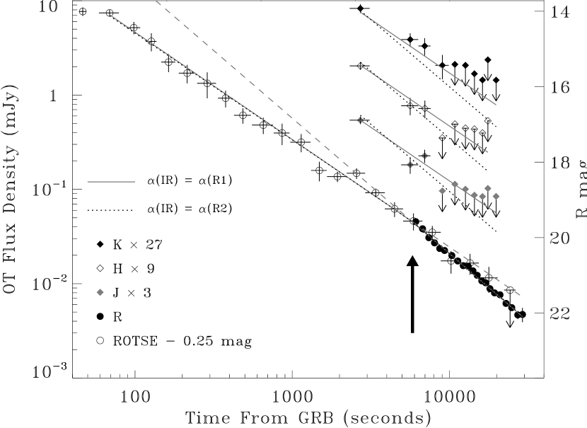
Figure 1: Lightcurves of the optical-IR data presented in this paper. These are converted to fluxes as described in §4, and the $J$, $H$, and $K_{s}$ bands are offset by factors of 3, 9, and 27 respectively for clarity. The ROTSE points are unfiltered and calibrated to $R$ ($C_{R}$). These points are offset by a color term of 0.25 magnitudes, a value determined from the $R$/$C_{R}$-band fit (see §4). Two fit models from Table 2 are overplotted. Each fits the bands simultaneously, scaling flux density $f_{\nu}\propto\nu^{\beta}t^{\alpha}$, with a break in $R$. The magnitude of the $R$ lightcurve break matches the passage of the cooling frequency $\nu_{c}$. The solid fit requires $\alpha(IR)=\alpha_{R1}$, the initial $R$-band decay, and the dotted fit requires $\alpha(IR)=\alpha_{R2}$, the final $R$-band decay. The dashed grey lines show the extrapolations of the initial and final $R$ temporal power laws (solid fit), and the arrow denotes the break time. Both fits are reasonable; $\alpha(IR)=\alpha_{R1}$ is expected for an ISM model, and $\alpha(IR)=\alpha_{R2}$ for a Wind. However, the $\alpha(IR)=\alpha_{R2}$ fit underestimates the $K_{s}$ data.

The lightcurves are plotted in Figure 1. The $R$-band lightcurve appears to be a broken power law. The need for a break is made obvious by the precise MDM observations at later times. The first (ROTSE) point in the lightcurve at $t-t_{GRB}=44$ s seems underluminous relative to subsequent decay. The IR data are less well-sampled, but can be described as a set of power laws with decay rates similar to those seen in the $R$ band.

To quantify these trends, we fit the data using power law and broken power law forms. The smooth broken power law form is

$$f(t)=f_{0}2^{1/s}((t/t_{b})^{-s\alpha_{1}}+(t/t_{b})^{-s\alpha_{2}})^{-1/s},$$ (1)

where $t_{b}$ is the break time, $f_{0}$ is the flux at the break time, $\alpha_{1}$ and $\alpha_{2}$ are the two power law indices, and $s$ is a sharpness parameter. The data (Fig. 1) clearly require a very sharp break transition. We use the form above for convenience, but do not fit the sharpness, setting $s$ at a very high value ($s=125$). As noted above, we also fit a constant multiplicative factor for the ROTSE $C_{R}$ points, as a color term. The ROTSE points after the break observed in the data have significant uncertainties. We expect any color change that may be associated with the break will not change the color term significantly in comparison to the ROTSE error bars.

The “separate” fit uses the form discussed above for the $R$-band data and individual power laws for each IR band (there is no substantial evidence for breaks in the IR data). This allows each band to have different temporal decays and flux normalizations.

The “multiband” fit connects the wavelength bands via a spectral index and coupled temporal decays, as expected in the fireball model. This fit uses the above functional form for $R$-band data, and simultaneously fits single power laws for the IR of the form

$$f(\nu_{i},t)=f_{0i}(\nu_{i}/\nu_{R})^{\beta}(t/t_{b})^{\alpha_{IR}},$$ (2)

where $\nu_{i}$ designates the frequency of an IR band. We attempt two “multiband” forms, $\alpha_{IR}=\alpha_{1}$ (the initial $R$-band decay index) and $\alpha_{IR}=\alpha_{2}$ (the final $R$-band decay index).

4.1 Early Underluminosity?

First, we examined the $R$-band lightcurve (ROTSE & MDM). A single power law does not produce an acceptable fit. We fit all $R$-band data (including “$C_{R}$”) to the “broken power law + color term” function described above, and repeated the exercise excluding the first point. Both produced formally acceptable fits, but excluding the first point improved the fit notably from $\chi^{2}=52.8$ for 39 degrees of freedom (DOF) to $\chi^{2}=44.9$ for 38 DOF.

The first observation, at 44 s post-GRB, appears to plateau, not joining the overall decay seen later. The flux density is approximately 4$\sigma$ below the back-extrapolation of the fit excluding the first point, marginal evidence for a deviation at early times from the later decay. While a single point cannot definitively establish such a deviation, the first point does not fit the overall later decay and thus we exclude it from the lightcurve fits discussed below and recorded in Table 2. The potential constraints placed by this first point are discussed later, in §5.2.

Overluminosity, or flux above the expectations from the subsequent decay, would be expected if a reverse shock’s emission were observable as it passes through the ejecta at early times comparable to our first observation (e.g., Mészáros & Rees, 1997; Sari & Piran, 1999). This is certainly not seen in our lightcurve. The maximum flux we observe in the first observation (99% confidence upper limit) is only 90% of the back-extrapolated flux from the fit excluding the first data point. A flux level significantly above this extrapolation would have been readily measurable.

4.2 Fitting the Frequency Bands Separately

The $R$ (& $C_{R}$) band, excluding the first point, were fit to the broken power law as described above, and each of the $J$, $H$, and $K_{s}$ bands were independently fit to a power law. Nondetections are included as flux densities of $0\pm f(m_{lim})$ to force the fit not to overestimate undetected fluxes. However, the elimination of nondetections from the fits does not change the parameters significantly. The resulting fit parameters are given in Table 2. Overall, the total $\chi^{2}=60$ for 61 DOF.

Due to the Ly$\alpha$ absorption discussed above, the $R$-band fit requires a significant color term, 0.25 magnitudes, for the ROTSE $C_{R}$ data relative to the filtered MDM $R$ measurements. With this systematic correction, the $R$-band lightcurve has a sharp break at a time $5700\pm 800$ s post-burst. The $R$-band lightcurve break is from a decay index $\alpha$ of $-1.13\pm 0.02$ to $-1.44\pm 0.02$, a $\Delta\alpha=-0.31\pm 0.03$. In the fireball model, the expected steepening from a “jet break” (observing a lack of flux due to the edge of conical ejecta) is at least $\Delta\alpha=-0.75$ (Panaitescu & Mészáros, 1999; Sari et al., 1999). The only shallow steepening expected in the fireball model is from the passage of the cooling frequency. The model predicts $\Delta\alpha(\nu_{c}=\nu)=-0.25$, consistent with the observed break at the $1.8\sigma$ level.

The NIR data are consistent with power law fits. The fitted $J$, $H$, and $K_{s}$ decay rates lie between the initial and final $R$-band decay rates. They are internally consistent at the 1$\sigma$ level and thus show no evidence for NIR color changes. The NIR decay indices are not as tightly constrained as those describing the $R$-band, with individual uncertainties $\delta\alpha\approx 0.2$. As the $R$-band break is shallow, each NIR band’s decay is consistent with either the initial or the final $R$-band decay index (at the 1.6$\sigma$ level or better).

Consistency with the initial $R$-band decay would be expected for an ISM fireball in which $\nu_{c}$ drops as $\propto t^{-1/2}$, while consistency with the final $R$-band decay would be expected for a Wind fireball where $\nu_{c}$ rises as $\propto t^{1/2}$ (as reviewed by Piran, 2005). The $K_{s}$ band is slightly more consistent with the ISM picture than the Wind, the $H$ and $J$ with the Wind than the ISM.

As evident from the poorly-determined NIR decay rates, the NIR data do not have the sensitivity to determine the presence or absence of a lightcurve break as shallow as that observed in the $R$-band. Moreover, the NIR time coverage is from 2320 s to 20700 s and the observed $R$-band break is at $5700\pm 800$ s. Even if the NIR data were more sensitive, given the timing of the $R$-band lightcurve break, in the ISM (Wind) model prediction, $\nu_{c}$ would not be observed falling (rising) to (from) the $J$ band during the NIR coverage. The ISM model would predict that $\nu_{c}$ would fall from $R$ to $J$ only at $t\sim 21000\pm 3000$ s. The Wind model would predict that $\nu_{c}$ would rise from $J$ to $R$, with the break in $J$ at $t\sim 1600\pm 200$ s.

4.3 Multiband Fitting

Given no obvious color changes, we also fit the multiband function as described in §§4.1, 4.2. We gave initial parameters to search for two cases, with the NIR decay either the power law behavior of the initial $R$-band lightcurve decay, or of the final $R$ decay. The two results are shown in Table 2. The $R$ decay indices, the $R$-band break time, and the $R$ flux at the break time do not change significantly. The break amplitude $\Delta\alpha$ is consistent with the cooling break passage at the 1.5$\sigma$ level in both cases.

Both multiband fits are formally quite good, with $\chi^{2}$/DOF$\approx$1. The data are insufficiently constraining to distinguish between $\alpha_{IR}=\alpha_{R1}$ (ISM expectation), and $\alpha_{IR}=\alpha_{R2}$ (Wind expectation). We show both of these fits in Figure 1, where the shallower $\beta$ favored by the $\alpha_{IR}=\alpha_{R2}$ model and the steeper IR decay make the fitted model underestimate all the $K_{s}$ data slightly. As the fit is nevertheless good, this only mildly favors $\alpha_{IR}=\alpha_{R1}$ and the ISM interpretation.

4.4 Spectral Index $\beta$

The optical-NIR spectrum of the data is well fit by a power law $f_{\nu}\propto\nu^{\beta}$. This is observed in the NIR data alone ($JHK_{s}$ at one common epoch), as well as $RJHK_{s}$ data (interpolating the $R$-band point). There is no significant change across observation epochs as there is no evidence for color changes from the lightcurves. The temporal decays of the IR bands are not strongly constrained ($\Delta\alpha\approx 0.2$, Table 2), are all mutually consistent, and are consistent (at $<2\sigma$) with either the initial or the final $R$-band decay. Moreover, the complete dataset is well fit by the “multiband” function that includes the spectral index $\beta$ to connect the bands.

The $JHK_{s}$ spectrum at the initial epoch yields $\beta=-0.9\pm 0.3$, while $RJHK_{s}$ gives $\beta=-0.9\pm 0.2$. These are not as well-constrained as the $\beta$ fit using the “multiband” function. When $\alpha_{IR}=\alpha_{R1}$, $\beta=-0.79\pm 0.05$ is fit, and when $\alpha_{IR}=\alpha_{R2}$, $\beta=-0.64\pm 0.06$.

These results are all mutually consistent. Given their variation, we take our measure of the optical-NIR spectral index to be $\beta=-0.8\pm 0.1$. The observed $R$-band lightcurve break will produce color changes relative to the single power laws of the NIR bands, but they are not detectable as we do not have good IR detections in the period from the break to the end of our NIR observations.

5 Discussion

The power law break in the $R$-band lightcurve is consistent with $\Delta\alpha=0.25$, the value expected for the passage of a cooling break $\nu_{c}$ in a fireball model with either an ISM or Wind circumburst density. The fireball model can also steepen a decay via a jet break, or via the passage of the typical frequency $\nu_{m}$ in the fast-cooling ($\nu_{c}<\nu_{m}$) case. The latter, for an observing frequency $\nu$, is the transition from $\nu_{c}<\nu<\nu_{m}$ to $\nu_{c}<\nu_{m}<\nu$. As previously noted, a jet break should be significantly steeper than the $\Delta\alpha\approx 0.3$ observed (Panaitescu & Mészáros, 1999; Sari et al., 1999). The $\nu_{m}$ passage in a fast-cooling case requires the initial decay to be $t^{-1/4}$ before the break (Piran, 2005, § VIIB) which is not compatible with any of the lightcurves.

From the temporal indices, we conclude that we are observing the passage of $\nu_{c}$ through $R$ at $t\approx 6000$ s. In the ISM case, this is a passage from $\nu_{m}<\nu(R)<\nu_{c}$ to $\nu_{m}<\nu_{c}<\nu(R)$. In the Wind case, it is from $\nu_{m}<\nu_{c}<\nu(R)$ to $\nu_{m}<\nu(R)<\nu_{c}$. Both require that $\nu_{m}$ is below the optical by the first fit data point at $t-t_{GRB}=59$ s.

5.1 Interpreting $\alpha$–$\beta$

The fireball model predicts relations between observed temporal and spectral indices and the value $p$ ($N(\gamma)\propto\gamma^{p}$) of the power law index for the spectral energy distribution of synchrotron-emitting electrons. The relations are functions of synchrotron spectral break ordering, the spectral segment, and whether the fireball is the ISM or Wind case, compiled by Piran (2005). With an initial and a final decay index, there are two relations to determine $p$ for each assumed case (ISM or Wind). Using the $R$-band decay indices from the “separate” fit gives values of $p$, $2.51\pm 0.03$ (from the initial $\alpha_{R1}$) and $2.58\pm 0.03$ (final $\alpha_{R2}$), for the constant-density ISM case, and $2.17\pm 0.03$ ($\alpha_{R1}$) and $2.25\pm 0.03$ ($\alpha_{R2}$), assuming the Wind case.

Given the relations between $p$ and $\alpha$, as well as those between $p$ and $\beta$, $\alpha$ and $\beta$ are related (again compiled in Piran, 2005, § VII). With the $R$ lightcurve break modelled by the passage of $\nu_{c}$ in either an ISM or a Wind-like medium, there are four possible $\alpha$–$\beta$ “closure” relations of $g(\alpha,\beta)=0$. We summarize them in Table 3, along with the values for the electron energy spectral index $p(\alpha)$ in these cases, and $p(\beta)$.

As before, the ISM model better represents the data. The ISM closure $g(\alpha,\beta)$ results are more consistent with 0, but the Wind cases do not deviate by more than $\approx 2\sigma$. Similarly, the values of $p$ inferred from the ISM relations $p(\alpha)$ better agree with its $p(\beta)$ than in the Wind case, with a similar level of consistency as the closure relations.

The observed spectral index of $-0.8\pm 0.1$ is consistent with either the ISM or Wind picture, as seen in the closure relations, but is slightly steeper than the Wind model expects (Table 3), by $\Delta\beta\approx 0.2$.

At the source redshift of $z=3.793$ (Prochaska et al., 2005), the $K_{s}$-band in the observer frame is roughly $B$-band in the local frame, and the $R$-band is near-UV at $2\times 10^{15}$ Hz. Over this frequency range in the source frame, a dust extinction law such as that of the Large Magellanic Cloud (LMC) will be linear, leading to a simple power law steepening of the spectrum (Fitzpatrick & Massa, 1988; Reichart, 2001). Dust extinction such as that observed in the Milky Way would have a significant bump in the middle of that frequency range, so we did not consider it. We use the LMC prescription of Reichart (2001) and determine that a small local extinction $A(V)\approx 0.1$ would give $\Delta\beta=0.2$. The amount of extinction would be sufficient to provide an intrinsic spectrum compatible with the Wind model. The extinction law prescribed for the Small Magellanic Cloud bar is steeper than the LMC case, and so if applicable should require less dust.

There cannot be a very large amount of extinction at the burst redshift. To get the observed spectrum with as little extinction as $A(V)=0.5$ requires a flat or rising intrinsic spectrum. Such an intrinsic spectrum is inconsistent with the fireball model.

Hurkett et al. (2005) present the Swift/XRT’s X-ray upper limits, from observations later than those presented here. We compare the X-ray limits to the optical by extrapolating the $R$-band flux density to their epoch, using our fitted models. We convert their flux limit to a spectral flux density limit using the spectral information given, both for their earliest epoch at $\sim 50$ ksec, and for the overall observation. We find that the early optical spectral index of $\beta=-0.8$ is marginally consistent with the X-ray limit, overestimating the X-ray 90% upper limit by approximately a factor of 3. (Given that the uncertainty is $\beta$ is 0.1, note that $\beta=-0.9$ would only overestimate the X-ray limit by a factor of 1.5, and $\beta=-0.95$ would match it.) The expected initial intrinsic $\beta=-0.8$ (ISM model; Table 3) would be marginally consistent, but the expected $\beta=-0.6$ (Wind; Table 3) would be inconsistent, overestimating the X-ray limit by at least a factor of 14.

This X-ray–optical spectrum is consistent with the passage of $\nu_{c}$. With an ISM model, $\nu_{c}$ has passed below the optical, steepening the spectrum between $R$ and the X-ray at later times. With a Wind profile, $\nu_{c}$ increases with time, placing it between $R$ and the X-ray at the time of the X-ray limit. However, $\nu_{c}$ would not get far above the optical and the spectrum steepens between $\nu_{c}$ and the X-ray. In both cases, the steepening $\Delta\beta=-0.5$ above $\nu_{c}$ results in a model-predicted X-ray flux well below the Swift/XRT limit.

5.2 Fireball Model Constraints

If the sub-luminosity of the earliest $R$-band observation (44 s) were known to be due to the passage of the peak $\nu_{m}$, there would be three numerical constraints for the fireball model’s spectral parameters: the peak time in $R$-band, the peak flux density value at that time, and the cooling break time at the $R$-band frequency. The early lightcurve behavior is neither strong evidence for a rollover from an earlier flatter lightcurve evolution, nor for a particular physical mechanism for a rollover. Therefore the first two constraints are inequalities; the peak $\nu_{m}$ could have have passed the optical band earlier.

The observed decay from $44$ to $6000$ s requires that the passage $\nu_{m}=\nu(R)$ is occurring or has occurred at $t\leq 44$ s. If $\nu_{m}$ passed the $R$-band before $44$ s, the synchrotron spectral peak would be at a lower frequency and a higher flux density than the $R$-band’s. Thus the peak flux density $f(\nu_{m})$ at $44$ s must be at least as bright as the initial $R$-band point.

The peak passage $\nu_{m}$ is quite early, having occurred at a time no later than 2.1 times the GRB duration measured by Gotz & Mereghetti (2005). The cooling break passage time of $\approx 5700$ s is significant, placing $\nu_{c}$ in the optical at a fairly early time. This is quite early in comparison to several other cases where broadband data has indicated $\nu_{c}$ is above the optical at a time $\sim$ days post-burst, e.g., 970508 (Galama et al., 1998), 000301C (Berger et al., 2001), or 011211 (Jakobsson et al., 2003). The implication in the ISM case with $\nu_{c}\propto t^{-1/2}$ would be a low value of $\nu_{c}$ during the first observation, with $\nu_{c}\sim 5\times 10^{15}$Hz at $44$ s.

We consider the observational constraints in light of both the ISM and the Wind models for the data. The synchrotron spectrum of a spherical fireball expanding into the ISM at a known redshift depends upon five parameters: energy $E$, density $n$, the power law slope of the electron energy distribution $p$, the energy fraction partitioned to the electrons, $\epsilon_{e}$, and the energy partition to the magnetic fields, $\epsilon_{B}$ (see Piran, 2005, and references therein). With three constraints and the value of $p$, we can put three of $E$, $n$, $\epsilon_{B}$, and $\epsilon_{e}$ in terms of the fourth, thus placing a limit upon a combination of two parameters.

We use the equations of Granot & Sari (2002) for the ISM slow-cooling case for $\nu_{m}$, $\nu_{c}$, and $F_{\nu_{m}}$. Adopting $p=2.55$, we find the numerical relations using the redshift $z=3.793$ (Prochaska et al., 2005) and a cosmology with $\Omega_{m}=0.3$, $\Omega_{\Lambda}=0.7$, $H_{o}=65$ km s^-1Mpc^-1 to determine the appropriate luminosity distance. We can then isolate

$$(\epsilon_{e}/0.1)(\epsilon_{B}/0.01)^{1/3}\leq 0.024,$$ (3)

where $\epsilon_{e}$ and $\epsilon_{B}$ are scaled to 10% and 1% respectively as these are reasonable expectations for the parameters from broadband fits in many afterglow cases (see, e.g., Panaitescu & Kumar, 2002; Yost et al., 2003). Within the simple fireball model that well-describes this afterglow case in the optical-IR, the implication is that the microphysical energy partitions must be quite small. For example, if $\epsilon_{e}=1\%$, then $\epsilon_{B}=0.01\%$. Other parameters can be put in terms of these, thus density $n\propto\epsilon_{B}^{-10/6}$. Keeping $n<100$ cm^-3 requires $\epsilon_{B}$ to be not much less than 1%.

We note that the microphysical parameter combination in eq. 3 is proportional to the peak flux density at 44 s as $F_{\nu_{m}}^{-1/3}$, and to the frequency of the peak $\nu_{m}$ at 44 s as $\nu^{1/2}$. Thus if the peak was significantly below the $R$ band at that time, this combination of microphysical parameters would be notably smaller.

For a Wind model, the physical parameter set is the same except that the density is parameterized by $A_{*}$, where $\rho=5\times 10^{11}A_{*}r^{-2}$ g cm^-1. We do a similar analysis using Granot & Sari (2002)’s equations. In this case, we find

$$(\epsilon_{e}/0.1)(\epsilon_{B}/0.01)^{1/3}\leq 0.08.$$ (4)

Once again the microphysical parameters must be small (and increasingly small as the initial value of $\nu_{m}$ is placed further below the $R$-band frequency).

There is an additional constraint:

$$A_{*}\geq 0.0004(\epsilon_{e}/0.1)^{2}.$$ (5)

This inequality indicates that, if $\nu_{m}<\nu(R)$ at the initial observation, $A_{*}(\epsilon_{e}/0.1)^{-2}$ would be larger than 0.0004. However, from the previous relation the low $\nu_{m}$ would require smaller microphysical parameters, $\epsilon_{e}$ or $\epsilon_{B}$ or both. If $\epsilon_{e}$ is decreased in the case $\nu_{m}<\nu(R)$, then $A_{*}$ would remain low. A value $A_{*}=0.0004$ is a very small wind outflow parameter; $A_{*}\sim 1$ is observed in Wolf-Rayet stars (as reviewed by Willis, 1991). The physical parameter constraints are somewhat easier to fulfill with the ISM fireball model than with the Wind model.

6 Conclusions

We observe a shallow break of $\Delta\alpha\approx 0.3$ in the $R$ lightcurve of the GRB 050502A afterglow at approximately 6000 s post-burst. We note that $J$, $H$, and $K_{s}$ observations during this period, not as well-sampled, do not constrain the presence or absence of such a lightcurve break in the NIR. With the shallow $\Delta\alpha$, we conclude that the optical break represents the passage of the synchrotron cooling frequency $\nu_{c}$ through $R$.

The observed spectral index is $\beta=-0.8\pm 0.1$. This is consistent with an ISM model for the broken $R$-band lightcurve, and slightly steeper than expected in a Wind model. The temporal and spectral index closure relations slightly favor an ISM over a Wind interpretation. A small amount of dust at the host redshift would steepen an intrinsically flatter spectrum sufficiently to accomodate the Wind interpretation.

There is no evidence for an overluminosity at our earliest observation, 44 s after the initial gamma-rays. The first lightcurve point appears suppressed, but from a single point we cannot conclude that this is the case. At a minimum, the early decay requires $\nu_{m}$ at or below $\nu(R)$ at that time. Using that constraint and the observation of $\nu_{c}$’s passage indicates that in both the ISM and the Wind explanations small microphysical energy partitions are required. The Wind interpretation expects an exceptionally low wind outflow parameter $A_{*}$, which may again somewhat favor an ISM interpretation.

Guidorzi et al. (2005) find multicolor evidence for a lightcurve bump at $t\approx 1700-3400$ s. A single ROTSE data point during this period has a slight rise above the overall decay, but not at a significant level given its signal to noise. $JHK_{s}$ sampling is insufficient to address whether the bump occurs at these wavelengths. Without the well-sampled MDM $R$-band observations presented here from 5800-28000 s, Guidorzi et al. (2005) did not detect the passage of $\nu_{c}$ through $R$.

Guidorzi et al. (2005) find the data favors a density variation over a refreshed shock as the source of the bump. In that case, the significance of the bump is greater than expected for $\nu(R)>\nu_{c}$ (see Nakar & Piran, 2003). For the Wind case the cooling break passage observed in the dataset presented here would be from $\nu(R)>\nu_{c}$ to $\nu(R)<\nu_{c}$ at $\approx$6000 s, so this again favors an ISM over a Wind interpretation.

We note that the observed steeper, steady decay following the lightcurve break is evident in the data over at least 0.7 logarithmic decades in time. Despite the evidence for a density variation in the data of Guidorzi et al. (2005), such an impulsive event cannot explain the sustained change in lightcurve evolution seen here.

There are several lines of evidence, including the spectral index, the closure relations of spectral and temporal indices, and the optical bump seen by Guidorzi et al. (2005), that all somewhat favor an ISM model over a Wind one for this afterglow.

With Swift and INTEGRAL providing rapid triggers, and rapid response instruments such as ROTSE and PAIRITEL providing followup, the GRB community is accumulating bursts with prompt, detailed observations. Such data sets should further probe the physics of GRB afterglows.

Table 1: Optical Photometry for GRB 050502A

Telescope	Filter	$t_{\mathrm{start}}$ (s)	$t_{\mathrm{end}}$ (s)	Magnitude
ROTSE-IIIb	None	44.0	49.0	$14.28\pm 0.11$
ROTSE-IIIb	None	59.0	78.9	$14.32\pm 0.09$
ROTSE-IIIb	None	88.5	108.0	$14.71\pm 0.16$
ROTSE-IIIb	None	117.2	136.8	$15.08\pm 0.23$
ROTSE-IIIb	None	146.7	180.5	$15.63\pm 0.23$
ROTSE-IIIb	None	190.0	239.6	$15.92\pm 0.24$
ROTSE-IIIb	None	248.7	327.7	$16.19\pm 0.33$
ROTSE-IIIb	None	337.5	416.7	$16.58\pm 0.22$
ROTSE-IIIb	None	426.5	546.1	$17.04\pm 0.20$
ROTSE-IIIb	None	555.3	754.4	$17.30\pm 0.21$
ROTSE-IIIb	None	763.6	962.7	$17.50\pm 0.28$
ROTSE-IIIb	None	971.9	1309.9	$17.75\pm 0.24$
ROTSE-IIIb	None	1319.7	1658.2	$18.50\pm 0.25$
ROTSE-IIIb	None	1667.4	2214.4	$18.66\pm 0.13$
ROTSE-IIIb	None	2224.1	2908.7	$18.57\pm 0.14$
ROTSE-IIIb	None	2918.0	3881.3	$19.09\pm 0.11$
ROTSE-IIIb	None	3890.5	5075.0	$19.52\pm 0.19$
ROTSE-IIIb	None	5084.1	6741.0	$19.84\pm 0.22$
ROTSE-IIIb	None	6750.1	8823.3	$20.14\pm 0.18$
ROTSE-IIIb	None	8832.5	11670.7	$20.90\pm 0.29$
ROTSE-IIIb	None	11680.6	15415.2	$20.95\pm 0.27$
ROTSE-IIIb	None	15425.1	20274.6	$21.34\pm 0.33$
ROTSE-IIIb	None	20284.1	28421.6	$<21.67$
MDM	$R$	5816.0	6416.0	$19.61\pm 0.03$
MDM	$R$	6458.0	7058.0	$19.79\pm 0.03$
MDM	$R$	7105.0	7705.0	$20.03\pm 0.03$
MDM	$R$	7750.0	8350.0	$20.17\pm 0.03$
MDM	$R$	8386.0	8986.0	$20.32\pm 0.03$
MDM	$R$	9025.0	9625.0	$20.37\pm 0.04$
MDM	$R$	9928.0	10828.0	$20.50\pm 0.04$
MDM	$R$	10871.0	11771.0	$20.65\pm 0.04$
MDM	$R$	11812.0	12712.0	$20.77\pm 0.06$
MDM	$R$	12750.0	13650.0	$20.79\pm 0.08$
MDM	$R$	13687.0	14587.0	$20.91\pm 0.06$
MDM	$R$	14621.0	15461.0	$21.03\pm 0.06$
MDM	$R$	15645.0	16545.0	$21.17\pm 0.06$
MDM	$R$	16587.0	17487.0	$21.23\pm 0.06$
MDM	$R$	17537.0	18737.0	$21.38\pm 0.06$
MDM	$R$	18797.0	19997.0	$21.49\pm 0.06$
MDM	$R$	20115.0	21915.0	$21.54\pm 0.05$
MDM	$R$	22041.0	23841.0	$21.77\pm 0.06$
MDM	$R$	24057.0	25857.0	$21.88\pm 0.08$
MDM	$R$	26358.0	28158.0	$22.08\pm 0.11$
MDM	$R$	28319.0	30119.0	$22.07\pm 0.19$
PAIRITEL	$J$	2322.5	3112.4	$17.38\pm 0.10$
PAIRITEL	$J$	4942.0	6335.4	$18.56\pm 0.21$
PAIRITEL	$J$	6365.4	7583.0	$18.32\pm 0.17$
PAIRITEL	$J$	8158.9	9903.5	$<19.25$
PAIRITEL	$J$	9970.9	11722.3	$<19.07$
PAIRITEL	$J$	11790.4	13538.4	$<19.21$
PAIRITEL	$J$	13568.0	15316.8	$<19.36$
PAIRITEL	$J$	15382.5	17134.5	$<19.40$
PAIRITEL	$J$	17201.3	17979.7	$<19.18$
PAIRITEL	$J$	18951.5	20742.1	$<19.40$
PAIRITEL	$H$	2322.5	3112.4	$16.64\pm 0.10$
PAIRITEL	$H$	4942.0	6335.4	$17.70\pm 0.23$
PAIRITEL	$H$	6365.4	7583.0	$17.77\pm 0.23$
PAIRITEL	$H$	8150.3	9903.5	$<18.55$
PAIRITEL	$H$	9970.9	11722.3	$<18.19$
PAIRITEL	$H$	11790.4	13538.4	$<18.30$
PAIRITEL	$H$	13568.0	15316.8	$<18.32$
PAIRITEL	$H$	15382.5	17134.5	$<18.42$
PAIRITEL	$H$	17201.3	17979.7	$<18.10$
PAIRITEL	$K_{s}$	2322.5	3112.4	$15.85\pm 0.11$
PAIRITEL	$K_{s}$	4942.0	6335.4	$16.67\pm 0.18$
PAIRITEL	$K_{s}$	6365.4	7583.0	$16.84\pm 0.22$
PAIRITEL	$K_{s}$	8150.3	9903.5	$17.36\pm 0.31$
PAIRITEL	$K_{s}$	9970.9	11722.3	$<17.33$
PAIRITEL	$K_{s}$	11790.4	13538.4	$<17.35$
PAIRITEL	$K_{s}$	13568.0	15316.8	$<17.57$
PAIRITEL	$K_{s}$	15382.5	17134.5	$<17.74$
PAIRITEL	$K_{s}$	17201.3	17979.7	$<17.21$
PAIRITEL	$K_{s}$	18951.5	20742.1	$<17.74$

Note. — All times are in seconds since the burst time, 02:13:57 UT (see § 2)

Table 2: Fit Parameters and $\chi^{2}$

Parameter	description	fit value	units
Fits to the Individual Bands
$\alpha_{R1}$	early $R$ power law index	$-1.131\pm 0.023$	-
$\alpha_{R2}$	late $R$ power law index	$-1.437\pm 0.022$	-
$t_{b}$	$R$ break time	$5690\pm 750$	sec
$f_{0,R}(t_{b})$	$f_{\nu}(R)$ at $t_{b}$	$46.7\pm 8.7$	$\mu$Jy
$\kappa$	ROTSE color term	$-0.250\pm 0.073$	mag
$\chi^{2}_{R}$	$\chi^{2}$ of $R$ fit/DOF	44.9/38	-
$\alpha_{J}$	$J$ power law index	$-1.33\pm 0.18$	-
$F_{J}$($t_{0}$)	$f_{\nu}(J)$ of 1st IR epoch	$182\pm 16$	$\mu$Jy
$\chi^{2}_{J}$	$\chi^{2}$ of $J$ fit/DOF	8.0/8	-
$\alpha_{H}$	$H$ power law index	$-1.36\pm 0.21$	-
$F_{H}$($t_{0}$)	$f_{\nu}(H)$ of 1st IR epoch	$229\pm 21$	$\mu$Jy
$\chi^{2}_{H}$	$\chi^{2}$ of $H$ fit/DOF	3.6/7	-
$\alpha_{K_{s}}$	$K_{s}$ power law index	$-1.17\pm 0.17$	-
$F_{K_{s}}$($t_{0}$)	$f_{\nu}(K_{s})$ of 1st IR epoch	$316\pm 32$	$\mu$Jy
$\chi^{2}_{K_{s}}$	$\chi^{2}$ of $K_{s}$ fit/DOF	3.4/8	-
Multiband Fit: NIR decay index = $\alpha_{R1}$
$\alpha_{R1}$	early power law index	$-1.137\pm 0.022$	-
$\alpha_{R2}$	late power law index ($R$ only)	$-1.435\pm 0.022$	-
$t_{b}$	$R$ break time	$5830\pm 250$	sec
$f_{0,R}(t_{b})$	$f_{\nu}(R)$ at $t_{b}$	$45.2\pm 2.8$	$\mu$Jy
$\beta$	spectral index $\nu^{\beta}$	$-0.785\pm 0.052$	-
$\kappa$	ROTSE color term	$-0.263\pm 0.066$	mag
$\chi^{2}$	$\chi^{2}$ of multiband fit/DOF	65.7/66	-
Multiband Fit: NIR decay index = $\alpha_{R2}$
$\alpha_{R1}$	early power law index ($R$ only)	$-1.131\pm 0.024$	-
$\alpha_{R2}$	late power law index	$-1.425\pm 0.022$	-
$t_{b}$	$R$ break time	$5600\pm 1800$	sec
$f_{0,R}(t_{b})$	$f_{\nu}(R)$ at $t_{b}$	$47\pm 21$	$\mu$Jy
$\beta$	spectral index $\nu^{\beta}$	$-0.641\pm 0.055$	-
$\kappa$	ROTSE color term	$-0.252\pm 0.096$	mag
$\chi^{2}$	$\chi^{2}$ of multiband fit/DOF	68.2/66	-

Table 3: Closure Relations for ($R$-band) Decay Index $\alpha$, Spectral Index $\beta$

Model	Relation (= 0)	Result	$p(\alpha)$	$p(\beta)$	expected $\beta(p(\alpha))$
ISM, initially $\nu_{m}<\nu(R)<\nu_{c}$	$\alpha_{1}-1.5\beta$	$0.07\pm 0.15$	$2.51\pm 0.03$	$2.6\pm 0.2$	$-0.76\pm 0.02$
ISM, initially $\nu_{m}<\nu(R)<\nu_{c}$	$\alpha_{2}-1.5\beta+0.25$	$0.01\pm 0.15$	$2.58\pm 0.03$		$-0.79\pm 0.02$
Wind, initially $\nu_{m}<\nu_{c}<\nu(R)$	$\alpha_{1}-1.5\beta+0.25$	$0.32\pm 0.15$	$2.17\pm 0.03$		$-0.59\pm 0.02$
Wind, initially $\nu_{m}<\nu_{c}<\nu(R)$	$\alpha_{2}-1.5\beta+0.5$	$0.26\pm 0.15$	$2.25\pm 0.03$	$2.6\pm 0.2$	$-0.63\pm 0.02$

Note. — The values of $\alpha_{1}$ is $\alpha_{R1}$, and $\alpha_{2}$ is $\alpha_{R2}$ from the Table 2 fit to the individual bands. $\beta$ is $-0.8\pm 0.1$ as determined in §4.4. The multiband fits also satisfy the closure relations given here.

References

- Akerlof et al. (2003) Akerlof, C. W., et al. Jan. 2003, PASP, 115, 132
- Berger et al. (2001) Berger, E., et al. Aug. 2001, ApJ, 556, 556
- Berger et al. (2003) Berger, E., et al. Nov. 2003, Nature, 426, 154
- Bertin & Arnouts (1996) Bertin, E. & Arnouts, S. June 1996, A&AS, 117, 393
- Bessell (1979) Bessell, M. S. Oct. 1979, PASP, 91, 589
- Cohen et al. (2003) Cohen, M., Wheaton, W. A., & Megeath, S. T. Aug. 2003, AJ, 126, 1090
- Fitzpatrick & Massa (1988) Fitzpatrick, E. L. & Massa, D. May 1988, ApJ, 328, 734
- Fruchter & Hook (1997) Fruchter, A. & Hook, R. N. 1997, in Applications of Digital Image Processing XX, Proc. SPIE, Vol. 3164, ed. , A. Tescher
- Galama et al. (1998) Galama, T. J., Wijers, R. A. M. J., Bremer, M., Groot, P. J., Strom, R. G., Kouveliotou, C., & van Paradijs, J. June 1998, ApJ, 500, L97+
- Gotz & Mereghetti (2005) Gotz, D. & Mereghetti, S. 2005, GCN Circ. No. 3329
- Gotz et al. (2005) Gotz, D., Mereghetti, S., Mowlavi, N., Shaw, S., Beck, M., & Borkowski, J. 2005, GCN Circ. No. 3323
- Granot & Sari (2002) Granot, J. & Sari, R. Apr, 2002, ApJ, 568, 820
- Guidorzi et al. (2005) Guidorzi, C., et al. July 2005, ApJL accepted, astro-ph/0507639
- Henden (2005) Henden, A. 2005, GCN Circ. No. 3454
- Huang et al. (2005) Huang, K. Y., et al. Aug. 2005, ApJ, 628, L93
- Hurkett et al. (2005) Hurkett, C., Page, K., Osborne, J. P., Zhang, B., Kennea, J., Burrows, D. N., & Gehrels, N. 2005, GCN Circ. No. 3374
- Jakobsson et al. (2003) Jakobsson, P., et al. Sept. 2003, A&A, 408, 941
- Landsman (1995) Landsman, W. B. 1995, , in ASP Conf. Ser. 77: Astronomical Data Analysis Software and Systems IV
- Mészáros & Rees (1997) Mészáros, P. & Rees, M. J. Feb. 1997, ApJ, 476, 232
- Mészáros et al. (1998) Mészáros, P., Rees, M. J., & Wijers, R. A. M. J. May 1998, ApJ, 499, 301
- Nakar & Piran (2003) Nakar, E. & Piran, T. Nov. 2003, ApJ, 598, 400
- Panaitescu & Kumar (2002) Panaitescu, A. & Kumar, P. June 2002, ApJ, 571, 779
- Panaitescu & Mészáros (1999) Panaitescu, A. & Mészáros, P. Dec. 1999, ApJ, 526, 707
- Piran (2005) Piran, T. 2005, Reviews of Modern Physics, 76, 1143
- Prochaska et al. (2005) Prochaska, J. X., Ellison, S., Foley, R. J., Bloom, J. S., & Chen, H.-W. 2005, GCN Circ. No. 3332
- Reichart (2001) Reichart, D. E. May 2001, ApJ, 553, 235
- Sari & Piran (1999) Sari, R. & Piran, T. Aug. 1999, ApJ, 520, 641
- Sari et al. (1999) Sari, R., Piran, T., & Halpern, J. P. July 1999, ApJ, 519, L17
- Sari et al. (1998) Sari, R., Piran, T., & Narayan, R. Apr, 1998, ApJ, 497, L17
- Sato et al. (2003) Sato, R., Kawai, N., Suzuki, M., Yatsu, Y., Kataoka, J., Takagi, R., Yanagisawa, K., & Yamaoka, H. Dec. 2003, ApJ, 599, L9
- Schlegel et al. (1998) Schlegel, D. J., Finkbeiner, D. P., & Davis, M. June 1998, ApJ, 500, 525
- Stetson (1987) Stetson, P. B. Mar. 1987, PASP, 99, 191
- Willis (1991) Willis, A. J. 1991, , in IAU Symp. 143: Wolf-Rayet Stars and Interrelations with Other Massive Stars in Galaxies
- Yost et al. (2003) Yost, S. A., Harrison, F. A., Sari, R., & Frail, D. A. Nov. 2003, ApJ, 597, 459
- Yost et al. (2005) Yost, S. A., Swan, H., Schaefer, B. A., & Alatalo, K. 2005, GCN Circ. No. 3322