The environmental dependence of clustering in hierarchical models

Abstract

In hierarchical models, density fluctuations on different scales are correlated. This induces correlations between dark halo masses, their formation histories, and their larger-scale environments. In turn, this produces a correlation between galaxy properties and environment. This correlation is entirely statistical in nature. We show how the observed clustering of galaxies can be used to quantify the importance of this statistical correlation relative to other physical effects which may also give rise to correlations between the properties of galaxies and their surroundings. We also develop a halo model description of this environmental dependence of clustering.

1
Introduction

A number of physical mechanisms are expected to play a role in determining the properties of a galaxy: e.g., ram pressure stripping, harrassment, and strangulation  (Gunn & Gott, 1972; Farouki & Shapiro, 1980; Moore et al., 1996; Balogh & Morris, 2000). Many of these operate in dense environments. So the existence of a morphology–density relation—the fraction of galaxies which have elliptical rather than spiral morphologies is higher in denser regions (Dressler, 1980)—is not unexpected. For similar reasons, recent measurements of lower star-formation rates in denser regions, which appears to persist even at fixed morphology (Balogh et al., 2002; Gomez et al., 2003) and stellar mass (Kauffmann et al., 2004), are not unexpected. However, determining which, if any, of the physical mechanisms mentioned above is the dominant one is more difficult.

Hierarchical galaxy formation models have been rather successful at reproducing the morphology–density relation (e.g. Benson et al., 2001). In these models, a correlation between galaxy-type and environment arises even if none of the physical mechanisms mentioned above are present. The correlation is a consequence of the following assumptions. Gravity has transformed small fluctuations in the early Universe into the structures we see today. This transformation was hierarchical, in the sense that small virialized objects formed first, and then merged with one another to form more massive virialized objects at a later time. The virialized objects present at any given time, called dark matter haloes, are approximately 200 times denser than the background universe at the time (Gunn & Gott, 1972). Galaxies form from gas which cools within virialized dark matter haloes (White & Rees, 1978). The properties of a galaxy are determined entirely by the mass and formation history of the dark matter halo within which it formed (e.g. White & Frenk, 1991; Kauffmann et al., 1997; Somerville & Primack, 1999; Cole et al., 2000). Halo masses and formation histories are directly related to the structure of the initial density fluctuation field from which they formed (Press & Schechter, 1974; Lacey & Cole, 1993; Sheth, Mo & Tormen, 2001). In hierarchical models, there is a correlation between fluctuations on different scales, and this induces correlations between halo mass and/or formation and the larger scale environment of a halo (Mo & White, 1996; Lemson & Kauffmann, 1999; Sheth & Tormen, 2002). This, in turn, induces a correlation between galaxy-type and environment. This correlation is entirely statistical in nature. So it is interesting to ask if this statistical correlation is sufficient to explain most of the observed correlation between galaxy-type and environment.

The main goal of the present work is to show how analysis of the clustering of galaxies can be used to quantify the strength of this statistical correlation between galaxy properties and environment. The idea is to show the strength of the statistical effect alone: any discrepancy with observations can then be ascribed to the other physical processes (Sheth, Abbas & Skibba, 2004). Although our argument is general, we focus in particular on the two-point correlation function, $\xi(r)$, and show how it is expected to depend on environment if the only environmental effects on galaxy properties are those which arise from the statistics of the initial fluctuation field. The present analysis is intended to complement traditional measures of the environmental dependence of clustering which tend to focus on correlations between the distribution of an observable (e.g., the luminosity function, or the star formation rate, etc.) and the environment (see e.g. Yang et al., 2003; Mo et al., 2004; Kauffmann et al., 2004; Balogh et al., 2004; Blanton et al., 2004, for some recent analyses).

This paper is arranged as follows. Section 2 uses numerical simulations to illustrate how clustering is expected to depend on environment if the entire environmental depedence arises from the correlation between haloes and their environments. Section 2.1 shows the effect for dark matter. A simple toy model which captures most of the relevant features of this effect is presented in Section 2.2. Section 2.3 uses mock galaxy samples to show that the effect should be easily measured in surveys such as the SDSS. The final section summarizes our results and discusses some implications. An Appendix shows how to describe the effect using the language of the halo model (see Cooray & Sheth, 2002, for a review) of large scale structure.

2 Environmental dependence of $\xi$

Throughout, we show results for a flat $\Lambda$CDM model for which $(\Omega_{0},h,\sigma_{8})=(0.3,0.7,0.9)$ at $z=0$. Here $\Omega_{0}$ is the density in units of critical density today, the Hubble constant today is $H_{0}=100h$ km s^-1 Mpc^-1, and $\sigma_{8}$ describes the rms fluctuations of the initial field, evolved to the present time using linear theory, when smoothed with a tophat filter of radius $8h^{-1}$ Mpc. The GIF and VLS numerical simulations we use to illustrate our arguments were made available to the public by the Virgo consortium. Both were run with the same $\Lambda$CDM cosmology, but with slightly different parameterizations of the initial fluctuation spectrum. The GIF simulation had $256^{3}$ particles in a cubic box with sides $L=141h^{-1}$Mpc. The VLS simulation had $512^{3}$ particles in a cubic box with sides $L=479h^{-1}$Mpc.

2.1 Dark matter simulations

To illustrate how clustering depends on environment, we used the halo and particle distributions in the $\Lambda$CDM GIF simulations (Kauffmann et al., 1999). The simulations contain approximately 90,000 haloes which each have at least ten particles, where the virialized halos were found using a friends-of-friends group finding program. We defined the environment of a halo by using the mass $M_{R}$ within a sphere of radius $R$ centred on the halo. We set $R=5h^{-1}$ or $8h^{-1}$Mpc, but any value which is substantially larger than the typical virial radius (a few hundred kpc), but smaller than the scale on which the Universe is essentially homogeneous, will do. We then ranked all the haloes in decreasing order of $M_{R}$. The particles belonging to the top one-third of the haloes were labeled as belonging to densest environments, and the particles in the bottom one-third of the halo sample were labeled as belonging to the least dense environments. Finally, we computed the correlation function of particles belonging to the haloes in the densest and least dense regions. The results are shown in Figure 1.

There are obvious differences between the two correlation functions. The correlation function for the particles in dense regions extends to larger scales; if fit to a power-law, it would have a shallower slope. The next section describes a simple model for these differences. The smooth curves in the figure show the result of a more complete analytic model that is developed in Appendix A.

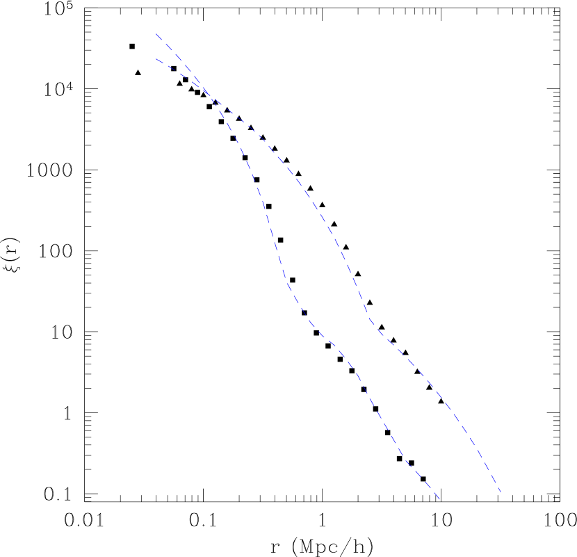
Figure 1: Environmental dependence of the dark matter correlation function in the $\Lambda$CDM GIF simulation. Triangles show $\xi(r)$ of particles in haloes which were defined as having the densest environments (defined by counting the mass within a sphere of radius of $5h^{-1}$Mpc centred on each halo), and squares are from particles in underdense regions. Smooth curves show the analytic model for this environmental effect that is developed in Appendix A.

2.2 A toy model

Let $dn(m,\delta_{c})/dm$ denote the number density of dark matter haloes with mass $m$ at a time when the linear theory overdensity required for spherical collapse is $\delta_{c}$, and let $N(m,\delta_{c}|M,V)$ denote the average number of $m$ haloes in regions of volume $V$ which contain mass $M$. Define $M/V\equiv\bar{\rho}(1+\delta)$, where $\bar{\rho}$ denotes the average density of the background. Dense regions have $\delta>0$. Mo & White (1996) showed that a generic feature of hierarchical models is that $N(m,\delta_{c}|M,V)\neq(1+\delta)\,V\,dn/dm$: i.e., dark halo abundances in dense and underdense regions do not differ by a simple factor which accounts for the difference in density. Rather,

$$N(m,\delta_{c}|M,V)\approx\Bigl{[}1+b(m)\delta\Bigr{]}V{dn(m,\delta_{c})\over dm},$$ (1)

where

$$b(m,\delta_{c})\approx 1-{d\ln dn(m,\delta_{c})/dm\over d\delta_{c}}$$ (2)

is a function which typically increases monotonically with $m$ (e.g. Sheth & Tormen, 1999). As a result, one expects the ratio of the number of massive to low mass haloes to be larger in dense regions than in less dense regions: the mass function in overdense regions should be ‘top-heavy’. Measurements in simulations indicate that this is indeed the case (e.g. Lemson & Kauffmann, 1999; Sheth & Tormen, 2002): the average halo mass increases with $\delta$.

In the GIF simulations, the average mass of the $\sim 30,000$ haloes which reside in the densest regions is approximately $m=2.5\times 10^{12}h^{-1}M_{\odot}$, whereas the average mass of the $\sim 30,000$ haloes which reside in the least dense regions is $m=5.2\times 10^{11}h^{-1}M_{\odot}$. (Hence, the two overdensities differed by a factor of approximately 5.)

The fact that dense regions have a top-heavy mass function has an important consequence for the environmental dependence of the correlation function which we now describe. Let $\xi(r|\delta)$ denote the shape of the correlation function in regions with overdensity $\delta$. Although such regions contain haloes with a range of masses, suppose we require that all haloes have the same mass $m_{\delta}$, chosen to match, say, the mean halo mass in the regions. If these haloes are not clustered, then $\xi(r|\delta)$ is simply a consequence of the shape of the density profiles $\rho(r|\delta)$ around haloes (Peebles, 1974):

$$\xi(r|\delta)=n_{clus}(m_{\delta})\int d{{\mbox{\boldmath$s$}}}\,{\rho({{\mbox{\boldmath$s$}}}|m_{\delta},\delta)\over\bar{\rho}_{\delta}}{\rho({{\mbox{\boldmath$s$}}}+{{\mbox{\boldmath$r$}}}|m_{\delta},\delta)\over\bar{\rho}_{\delta}},$$ (3)

where $n_{clus}(m_{\delta})$ is the average number density of haloes surrounded by regions with overdensity $\delta$, $\bar{\rho}_{\delta}\equiv m_{\delta}n_{clus}$, and $m_{\delta}\equiv\int d{{\mbox{\boldmath$s$}}}\,\rho({{\mbox{\boldmath$s$}}}|m_{\delta},\delta)$. In fact, the haloes are clustered, but Sheth & Jain (1997) show why ignoring halo clustering should be a good approximation on small scales. Hence, to estimate the small scale correlations as a function of environment, we require an estimate of the shapes of halo density profiles.

When fit to spherical models, the density profiles of haloes in simulations are well fit by the functional form $\rho(r|m)/\bar{\rho}=\Delta_{c}(r_{vir}/cr)/(1+cr/r_{vir})^{2}$ where $r_{vir}\equiv(3m/4\pi\Delta_{vir}\bar{\rho})^{1/3}$ and $c\equiv 9\,(10^{13}h^{-1}M_{\odot}/m)^{0.1}$ (Navarro et al., 1997). If we assume that the density profiles of $m$ haloes are the same in all environments (we will modify this assumption shortly), then $\xi(r|\delta)$ is given by inserting this expression for the density profile into the convolution integral above. The result is

$$\xi(r|\delta)={\Delta_{vir}\over\bar{\rho}_{\delta}/\bar{\rho}}\ \lambda(r|m_{\delta},\delta),\qquad{\rm provided}\quad r\leq 2r_{vir},$$ (4)

where $\lambda$ is a messy function of $c$ and $cr/r_{vir}$ (given in Sheth et al., 2001). Since $\Delta_{vir}$ is independent of $m$, in such a model, the environmental dependence of $\xi(r|\delta)$ comes entirely from the fact that dense regions host the more massive haloes, and halo density profiles depend on halo mass. The factor of $\bar{\rho}_{\delta}/\bar{\rho}$ in the denominator derives from the fact that haloes which have a fixed overdensity relative to the global background density $\bar{\rho}$ have a different overdensity relative to the local background $\bar{\rho}_{\delta}$.

Figure 2 shows the result of this simple analytic estimate of $\xi(r|\delta)$ for the two sets of GIF simulation particles: those which reside in the 30,000 haloes with the largest surrounding overdensities (as described previously), and those which reside in the 30,000 haloes with the smallest surrounding overdensities The curves are qualitatively similar to the measurements shown in Figure 1, at least out to scales on which the measurements show an inflection: $\xi$ falls to zero on smaller scales in the less dense regions. The inflections at $\sim 0.8h^{-1}$Mpc and $\sim 3h^{-1}$Mpc in the simulations (Figure 1) denote the scales which are approximately twice the virial radii of the typical haloes in the two regions. Beyond this scale, halo-halo correlations become important; we build a model for this in Appendix A.

Figure 2: The correlation function of particles in haloes which are surrounded by dense regions (curves which extend to larger $r$), and by less dense regions (curves which fall to zero at smaller $r$), in our toy model. The number of haloes in the two environments was assumed to be the same, but the halo mass in dense regions was assumed to be larger by a factor of 5. Solid curves have $c=10$ in both cases, whereas dashed curves include a realistic prescription for the weak mass dependence of $c$.

The curves which extend to larger scales are those for particles in the denser regions. This is easily understood, because dense regions are those for which $m_{\delta}$ is larger, and hence $r_{vir}$ is larger. The reason why $\xi(r|\delta)$ on small scales is larger for the less dense regions is more subtle.

The solid curves show results in which we have set $c=10$ and ignored the mass dependence of $c$, and dashed curves include the mass dependence but assume that there is no additional dependence on environment. Clearly, the mass dependence of $c$ is not a dominant effect even on scales smaller than $r_{vir}/c$. Thus, the difference in amplitudes on small scales derives from the factor of $\bar{\rho}_{\delta}/\bar{\rho}$ in the expression above, and not from the mass dependence of $c$. In the present example, the number of haloes in the two (dense and underdense) regions is the same, but $m_{\delta}$ in dense regions is larger, so $\bar{\rho}_{\delta}/\bar{\rho}$ is larger for the dense regions. Since the shape of $\xi$ is approximately constant on small scales, it has a lower amplitude in denser regions.

The relative unimportance of $c$ has the following interesting consequence. Suppose that halo density profiles do depend on environment (numerical simulations are only just reaching the resolution required to address this question). A simple way of parameterizing this dependence is to allow $c$ to depend both on $m$ and $\delta$. If $c$ depends only weakly on $\delta$, then the effect on $\xi$ will only be noticeable on scales smaller than $r_{vir}/\bar{c}$, where $\bar{c}$ denotes the mean $c$ (averaged over environments).

On the smaller scales, where halo-halo correlations are not important, the differences between the two curves in Figure 1 are qualitatively like those of the simple toy model described above, indicating that our use of a mean density-dependent halo mass $m_{\delta}$, rather than a distribution of masses, does capture the essential features of the density dependence of $\xi(r|\delta)$. On larger scales, where halo correlations are important, Figure 1 shows that $\xi(r|\delta)$ is stronger in dense regions. This is not unexpected in the context of the linear peaks-bias model of (Kaiser, 1984), if, on average, the densest regions at the present time formed from the densest regions in the initial fluctuation field. This is because, in the initial Gaussian random field, the densest regions were more strongly clustered than regions of average density. Therefore, our simple model, in which the environmental dependence of $\xi$ is entirely due to the environmental dependence of the halo mass function, suggests the following generic features for $\xi(r|\delta)$: on scales larger than the virial radius of a typical halo, the amplitude of $\xi$ should increase as $\delta$ increases; on smaller scales, the amplitude of $\xi$ in underdense regions should be larger; hence, the slope of $\xi$ in dense regions should be shallower than in less dense regions.

2.3 Mock galaxy samples

To illustrate that the features described above really are generic, and to make a closer connection to observations, we assigned mock ‘galaxies’ to haloes in the simulations as follows. Sufficiently low mass haloes contain no galaxies. Haloes more massive than some $m_{L}$ contain at least one galaxy. The first galaxy in a halo is called the ‘central’ galaxy. The number of other ‘satellite’ galaxies is drawn from a Poisson distribution with mean $N_{s}(m)$ where

$$N_{s}(m)=\left(\frac{m}{m_{1}}\right)^{\alpha}\text{ if }m\geq m_{L}.$$ (5)

This procedure is motivated by Kravtsov et al. (2004). We distribute the satellite galaxies in a halo around the halo centre so that the radial profile follows that of the dark matter (i.e., the galaxies are assumed to follow an NFW profile). We set $m_{L}=10^{11.27}h^{-1}M_{\odot}$, $m_{1}=23m_{L}$, and $\alpha=0.92$; Zehavi et al. (2004) show that this choice is appropriate for SDSS galaxies more luminous than $M_{r}<-18$. We then compute $N_{5}$, the number of galaxies in a $5h^{-1}$Mpc sphere around each galaxy, and rank the galaxies in order of decreasing $N_{5}$. The top one-third are labeled as being galaxies in dense regions, and the bottom third as being in underdense regions.

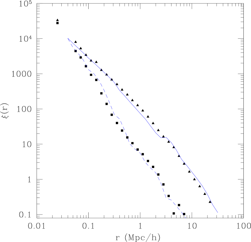
Figure 3: Similar to Figure 1, but now for model galaxies distributed according to the model described in the text around equation 5, and density defined by counting galaxies in spheres centred on the galaxies themselves, rather than the mass in spheres centred on haloes. Curves show the analytic model developed in Appendix A.

Figure 3 presents the correlation functions of the mock galaxies classified as being in dense (top) and underdense (bottom) regions. Once again we see the generic tendency for $\xi$ computed using objects in denser regions to be shallower than when objects in sparser environments are used.

The important point, which we note explicitly here, is the following: By assuming that equation (5) is the same function of $m$ for all environments, and by assuming that the radial profile of the galaxies depends only on halo mass and not on environment, we have constructed a galaxy catalog in which all environmental effects are entirely a consequence of the correlation between halo mass and environment. Therefore, the locii traced out by the two sets of symbols shown in Figure 3 represent the predicted environmental dependence of $\xi$ if there are no environmental effects other than the statistical one determined by the initial fluctuation field.

Over the $1-10h^{-1}$Mpc range which the SDSS data currently probe most reliably, $\xi$ for the dense and underdense samples differs by an order of magnitude. This difference is easily measurable in data sets which are currently available. Comparison of this predicted difference with measurements in the SDSS will provide a sharp test of the assumption that environmental effects are dominated by the statistical correlation between the halo mass function and environment, rather than by other ‘gastro’physics.

3 Discussion and Conclusions

In hierarchical models, the clustering of dark matter particles should be a strong function of environment. This is a consequence of the fact that massive haloes populate the densest regions. If the properties of galaxies are determined entirely by the masses and formation histories of the haloes in which they sit, then the clustering of galaxies should also depend strongly on environment.

We discussed a method for testing this assumption. The test is particularly interesting given recent work which suggests that, at fixed mass, haloes in dense regions form at higher redshifts (Sheth & Tormen, 2004), and that this effect is a decreasing function of halo mass (Gao, Springel & White, 2005). In particular, Section 2.3 described how to generate a mock galaxy catalog in which all correlations with environment are a consequence of the correlation between halo abundances and environment. Comparison of the environmental dependence of clustering in the mock catalog and in real data allows one to test the assumption that environmental effects are dominated by the statistical correlation between halo mass and environment.

The Appendix shows how to incorporate the assumption that environmental effects are determined entirely by the statistical correlation between halo mass and environment into the halo model description of large scale structure. While this model aids in understanding the effect, to perform the test with data, it is unnecessary—measurements of clustering in the mock catalogs of the sort described in Section 2.3 are sufficient. However, the methodology developed in this work provides a means for computing the clustering properties of galaxies affected by other environment dependent processes (assuming that some model for $\langle N_{gal}|m,M,V\rangle$ could be derived) that explicitly do not depend upon the surrounding halo mass. For instance, winds from galaxies in nearby clusters are assumed to depend on the larger scale environment and could affect the clustering statistics.

In particular, on scales larger than a Megaparsec or so, the two-point correlation function $\xi$ of galaxies surrounded by high density regions is predicted to be larger than for galaxies in less dense regions. In addition, the slope of $\xi$ for galaxies in dense regions should be shallower (cf. Figure 3). And if the distribution of galaxies around halo centers depends only weakly on environment (current analyses of galaxy clustering assume any such dependence is negligible), the effect on their clustering amplitude is small.

Our test using mock catalogs is unrealistic in one respect: with real data, one only has redshift-space positions, so one cannot define the local density in real-space. However, if the scale on which the redshift-space density is defined is larger than the typical size of redshift-space distortions ($\sim 5h^{-1}$Mpc), then the real and redshift-space densities will not differ substantially. Hence, we do not expect our separation into environments based on the real-space density within $8h^{-1}$Mpc spheres to differ substantially from that which we would have obtained had we used redshift-space positions instead. A more detailed description of the redshift space method is the subject of work in progress. (E.g., what does one gain by measuring both $\xi(s)$ and the projected correlation function as a function of redshift space environment? The latter quantity depends on local density for similar reasons that $\xi(r)$ does—the halo mass function depends on environment—whereas $\xi(s)$ will have an additional effect coming from the fact that redshift space distortions depend on halo mass.) Comparison of these predictions with clustering in the Sloan Digital Sky Survey is underway.

Appendix A An analytic model

This Appendix provides an analytic model which incorporates the assumption that environmental effects are determined entirely by the statistical correlation between halo mass and environment. Note that to perform the test with data, this analytic model is unnecessary—measurements of clustering in the mock catalogs described previously are sufficient.

The analysis which follows uses the framework of the halo model of large scale structure (see Cooray & Sheth, 2002, for a review). It extends that of the toy model described in the main text in two ways: it allows for a range of halo masses, and it allows for correlations between haloes.

A.1 The halo model for dark matter

In this model, all mass is bound up in dark matter haloes which have a range of masses. Hence, the background density is

$$\bar{\rho}=\int dm\,{dn(m)\over dm}\,m.$$ (6)

where $dn(m)/dm$ denotes the number density of haloes of mass $m$. The correlation function is the Fourier transform of the power spectrum $P(k)$:

$$\xi(r)=\int{dk\over k}\,{k^{3}P(k)\over 2\pi^{2}}\,{\sin kr\over kr}.$$ (7)

In the halo model, $P(k)$ is written as the sum of two terms: one that arises from particles within the same halo and dominates on small scales (the 1-halo term), and the other from particles in different haloes which dominates on larger scales (the 2-halo term). Namely,

$$P(k)=P_{1h}(k)+P_{2h}(k),$$ (8)

where

$$\begin{split}P_{1h}(k)&=\int dm\,{dn(m)\over dm}\,\frac{m^{2}}{\bar{\rho}^{2}}\,|u(k|m)|^{2},\\ P_{2h}(k)&=\left[\int dm\,{dn(m)\over dm}\,\frac{m}{\bar{\rho}}\,b(m)\,u(k|m)\right]^{2}P_{\rm Lin}(k).\end{split}$$ (9)

Here $u(k|m)$ is the Fourier transform of the halo density profile, $b(m)$ is the bias factor which describes the strength of halo clustering, and $P_{Lin}(k)$ is the power spectrum of the mass in linear theory. When explicit calculations are made, we assume that the density profiles of haloes have the form described by Navarro et al. (1997), and that halo abundances and clustering are described by the parameterization of Sheth & Tormen (1999):

$${m\over\bar{\rho}}\,{dn(m)\over dm}\,{\rm d}m = f(m)\,{\rm d}m=f(\nu)\,{\rm d}\nu$$

$$= {{\rm d}\nu^{2}\over\nu^{2}}\,\sqrt{a\nu^{2}\over 2\pi}\,\exp\left(-{a\nu^{2}\over 2}\right)A\,\left[1+(a\nu^{2})^{-p}\right]$$

$$b(m) = 1+{a\nu^{2}-1\over\delta_{\rm sc}}+{2p/\delta_{\rm sc}\over 1+(a\nu^{2})^{p}}$$

$$\nu = {\delta_{\rm sc}\over\sigma(m)}\quad{\rm and}$$

$$\sigma^{2}(m) = \int_{0}^{\infty}{{\rm d}k\over k}\,{k^{3}P_{\rm Lin}(k)\over 2\pi^{2}}\ W^{2}(kR_{0}),$$ (10)

where $W(x)=(3/x^{3})[\sin(x)-x\cos(x)]$ and $R_{0}=(3M/4\pi\bar{\rho})^{1/3}$. That is to say, $\sigma(M)$ is the rms value of the initial fluctuation field when it is smoothed with a tophat filter of comoving size $R_{0}$, extrapolated using linear theory to the present time. Here $\delta_{\rm sc}$ is the critical density required for spherical collapse, extrapolated to the present time using linear theory (it is 1.686 for an Einstein de-Sitter model), and $a\approx 0.71$, $p=0.3$ and $A=(1+\Gamma(1/2-p)/\sqrt{\pi}/2^{p})^{-1}\approx 0.322$. If $a=1$, $p=0$ and $A=1/2$, then ${\rm d}n/{\rm d}m$ is the same as the universal mass function first written down by Press & Schechter (1974).

A.2 Including the environmental effect

The expressions above are the result of averaging over environments. Including the environmental dependence of the halo distribution explicitly is not entirely straightforward, because, as we describe below, it requires knowledge of the probability that a region of volume $V$ has overdensity $\delta$. As we describe below, we use the excursion set model described in Sheth (1998) to do this.

In this model, spherical evolution is described by a ‘moving barrier’:

$$\delta_{0}(\Delta)={\delta_{\rm sc}\over 1.686}\,\Biggl{[}1.686-{1.35\over\Delta}-{1.124\over\Delta^{1/2}}+{0.788\over\Delta^{0.587}}\Biggr{]}$$ (11)

where $\Delta\equiv M/\bar{\rho}V$. This barrier is said to be ‘moving’ because, for general $V$, it is a function of $M$. The excursion set model attributes special significance to the first crossing distribution $f(M,V)dM$ of this barrier by Brownian motion random walks: it is a measure of the mass fraction in regions of size $V$ which contain mass $M$. In this approach, a halo can be thought of as a patch which has collapsed to vanishingly small volume. In the limit of $V\to 0$, $\delta_{0}\to\delta_{\rm sc}$ is the same constant for all $M$. In this limit the barrier is said to have constant ‘height’, and the first crossing distribution $f(M,\delta_{\rm sc})dM$ represents the mass fraction in haloes of mass $M$. Thus, $f(M,\delta_{\rm sc})$ equals $(M/\bar{\rho})$ times $dn(M,\delta_{\rm sc})/dM$, the halo mass function.

Notice that, for general $V$, $\delta_{0}(\Delta)\leq\delta_{\rm sc}$ for all $M$. Hence, $f(m,\delta_{\rm sc}|M,V)$, the first crossing distribution of $\delta_{\rm sc}$ by walks which first crossed the moving barrier associated with non-zero $V$ at $M$, denotes the mass fraction of cells of size $V$ which contain mass $M$ which is in haloes which have mass $m$ for some $m\leq M$. This fraction equals $(m/M)$ times $N(m,\delta_{\rm sc}|M,V)$, the environmental dependent mass function discussed in the main text (cf. equation 1).

In the main text (e.g. Section 2.1), we define the environment of a halo by considering the mass in a patch of volume $V$ surrounding it. To classify haloes by their environment, we must be able to estimate the number density of haloes of mass $m$ which are surrounded by regions of volume $V$ which contain mass $M$. If $dn(m)/dm$ denotes the number density of $m$ haloes, and $f(M,V|m)$ denotes the fraction of $m$ haloes which contain mass $M$ in the surrounding volume $V$, then the number density of such haloes is $f(M,V|m)\,dn(m)/dm$. In the excursion set model, this equals

$$\begin{split}{dn(m)\over dm}\,f(M,V|m)dM&={\bar{\rho}\over m}\,f(m)f(M,V|m)\,dM\\ &=\frac{\bar{\rho}}{m}\,f(M,V)f(m|M,V)\,dM\\ &=n(M,V)\,N(m|M,V)\,dM,\end{split}$$ (12)

where $f(M,V)dM$ is given by computing the first-crossing distribution of the moving barrier associated with spherical collapse described above. (In practice, we use the analytic approximation to the first crossing distribution of such moving barrier problems given by Sheth & Tormen, 2002).

The mass density contributed by haloes that are embedded in regions of mass $M_{min}\leq M\leq M_{max}$ is;

$$\bar{\rho}_{\delta} = \int_{M_{min}}^{M_{max}}dM\int_{0}^{M_{max}}dm\,{dn(m)\over dm}\,f(M,V|m)\,m$$ (13)

$$= \int_{M_{min}}^{M_{max}}\!\!\!\!\!\!\!dM\,n(M,V)\int_{0}^{M}dm\,N(m|M,V)\,m$$

$$= \int_{M_{min}}^{M_{max}}\!\!\!\!\!\!\!dM\,n(M,V)\,M.$$

In the standard model, the density profile of a halo depends on its mass, but not on the surrounding environment. In this case, the one-halo term is

$$\begin{split}P_{1h}(k|\delta)=&\int_{M_{min}}^{M_{max}}dM\,n(M,V)\\ \ &\times\int_{0}^{M}dm\,N(m|M,V)\left(\frac{m}{\bar{\rho_{\delta}}}\right)^{2}|u(k|m)|^{2}.\end{split}$$ (14)

This reduces to the standard 1-halo term in the limits $M_{min}\rightarrow 0$ and $M_{max}\to\infty$.

The two-halo term is more complex as it now has two types of contributions: pairs which are in the same patch (2-halo–1-patch), and pairs in different patches (2-halo–2-patch). The 2-halo–1-patch term can only be important on intermediate scales (i.e., those which are larger than the diameter of a typical halo but smaller than the diameter of a patch). It is more complex to model this term accurately, as we describe shortly. The 2-halo–2-patch term, on the other hand, is simpler. It should be well approximated by

$$\begin{split}{P_{2h-2p}(k|\delta)\over P_{\rm Lin}(k|R_{p})}&=\Biggl{[}\int_{M_{min}}^{M_{max}}dM\,n(M,V)\,B(M,V)\\ \ &\qquad\times\int_{0}^{M}\!\!dm\,N(m|M,V)\frac{m}{\bar{\rho_{\delta}}}\,u(k|m)\Biggr{]}^{2},\end{split}$$ (15)

where $P_{\rm Lin}(k|R_{p})$ denotes the power spectrum associated with setting the linear theory correlation function to $-1$ on scales smaller than the diameter of a patch $2R_{p}$. This truncation has little effect on small $kR_{p}\ll 1$, where $P_{\rm Lin}(k|R_{p})\approx P_{\rm Lin}(k)$. The factor $B(M,V)$ describes bias associated the clustering of the patches, and depends on the abundance of such patches in exactly the same way that $b(m)$ is related to $dn(m)/dm$ (c.f. equation 2). Note that this expression assumes that the 2-halo–2-patch term is given simply by weighting the patch-patch correlation by the halo abundance within a patch.

To a first approximation, patches do not overlap with one another, so the 2-halo–2-patch term should drop on scales smaller than the diameter of a patch. It is on these scales that $P_{2h-1p}$ should begin to dominate. A first approximation for the net effect of $P_{2h-1p}$, then, is to not enforce this small-scale decrease of $P_{2h-2p}$, and to simply use the expression above for $P_{2h-2p}$ but $P_{\rm Lin}(k)$ instead of $P_{\rm Lin}(k|R_{p})$, for all $k$. Section A.4 shows that this expression reduces to the standard two-halo term when $M_{min}\rightarrow 0$ and $M_{max}\rightarrow\infty$, so it is at least a reasonable approximation. However, we will see below that the correlation function of objects in underdense regions sometimes shows a clear signature of the fact that patches do not overlap. Thus, a more sophisticated approximation is required to describe clustering in underdense regions.

To estimate the 2-halo–1-patch term, it is convenient to think of the patches as haloes, and of the haloes as patch-substructure. Sheth & Jain (2003) have developed the halo model description of clustering when haloes have substructure. They allow for the possibility that a halo may be made up of a smooth component plus a population of subclumps. Our present case corresponds to assigning all the mass to subclumps, and none to the smooth component, so that only the final two of the four terms in their equation (31) contribute. Our expression for $P_{1h}(k|\delta)$ is effectively the same as their final term, so their third term is our $P_{2h-1p}(k|\delta)$. Namely,

$$\begin{split}P_{2h-1p}(k|\delta)&=\int_{M_{min}}^{M_{max}}dM\,n(M,V)\\ \ &\ \times\int_{0}^{M}dm_{1}\,\left(\frac{m_{1}}{\bar{\rho_{\delta}}}\right)|u(k|m_{1})|\\ \ &\ \times\int_{0}^{M-m}dm_{2}\,\left(\frac{m_{2}}{\bar{\rho_{\delta}}}\right)|u(k|m_{2})|\\ \ &\ \times\ N(m_{1},m_{2}|M,V)\ U(k|m_{1},m_{2},M)^{2}.\end{split}$$ (16)

Here $U$ denotes the normalized Fourier transform of the spatial distribution of $m_{1}$ and $m_{2}$ haloes within a patch. A simple first estimate would use the correlation function of the haloes to model this profile, but to truncate this at the patch radius, since both haloes are required to lie within the patch:

$$U^{2}\approx b(m_{1})b(m_{2})\,{P_{\rm Lin}(k)-P_{\rm Lin}(k|R_{p})\over M/\bar{\rho}}$$ (17)

where $P_{\rm Lin}(k)-P_{Lin}(k|R_{p})$ denotes the power spectrum associated with setting the linear theory correlation function to zero on scales larger than the diameter of a patch $2R_{p}$. The other term, $N(m_{1},m_{2}|M,V)$, denotes the average number of haloes of mass $m_{1}$ and $m_{2}$ in patches $V$ which contain total mass $M$. Sheth & Lemson (1999) argue that, as a consequence of mass conservation,

$$N(m_{1},m_{2}|M,V)\approx N(m_{1}|M,V)\,N(m_{2}|M-m_{1},V-v_{m_{1}}),$$ (18)

where $v_{m}$ is the volume associated with an $m$ halo.

When $M\gg m$ and $V\gg v_{m}$, as it is in large overdense regions, then $N(m_{1},m_{2}|M,V)\approx N(m_{1}|M,V)\,N(m_{2}|M,V)$ i.e, $N(m_{1},m_{2}|M,V)$ is well approximated by the product of the individual mean values. In this case,

$$\begin{split}{P_{2h-1p}(k|\delta)\over P_{\rm Lin}(k)-P_{\rm Lin}(k|R_{p})}\approx&\int_{M_{min}}^{M_{max}}dM\,{n(M,V)\over M/\bar{\rho}}\\ \ &\times\Biggl{[}\int_{0}^{M}dm\,N(m|M,V)\,b(m)\,\\ \ &\qquad\quad\times\left(\frac{m}{\bar{\rho_{\delta}}}\right)|u(k|m)|\Biggr{]}^{2}.\end{split}$$ (19)

In underdense regions, however, simply using the product of the individual mean values is expected to be a bad approximation.

The smooth curves in Figure 1 show that the model developed above provides a good description of the environmental dependence of the dark matter correlation function. In our comparisons, we have found that the full expression (equations 16–18) provides a substantially better description of $P_{2h-1p}$ in the underdense regions, whereas the simpler approximation of equation (19) is adequate for the dense regions.

A.3 From dark matter to galaxies

We now discuss how the model above can be extended to describe the environmental dependence of galaxy clustering. When all environments have been averaged over, the mean number density of galaxies $\bar{n}_{gal}$ is given by replacing the weighting by $m$ in equation (6) for the mean density by $\langle N_{gal}|m\rangle$, the mean number of galaxies in an $m$-halo. For instance, one could use equation (5) to write $\langle N_{gal}|m\rangle=1+\langle N_{s}|m\rangle$. Similarly, the weighting by $m/\bar{\rho}$ in $P_{2h}(k)$ is replaced with a weighting by $\langle N_{gal}|m\rangle/\bar{n}_{gal}$. And the weighting by $(m/\bar{\rho})^{2}$ in the 1-halo term becomes $[2\langle N_{s}|m\rangle\,u(k|m)+\langle N_{s}|m\rangle^{2}\,|u(k|m)|^{2}]/n_{gal}^{2}$. This weighting assumes there is always one galaxy at the centre, and that the number of satellite galaxies in an $m$-halo follows a Poisson distribution with mean $\langle N_{s}|m\rangle$.

If one had an estimate of the dark matter density field, then one could include the environmental dependence of galaxy clustering by writing the mean number of galaxies in an $m$-halo surrounded by a region $V$ containing mass $M$ as $\langle N_{gal}|m,M,V\rangle$. If this mean number did not depend on $M$ and $V$, then the environmental dependence of galaxy clustering would be described by making the same replacements in the expressions for $P(k|\delta)$ as one makes for $P(k)$.

In practice, one observes galaxies, not dark matter, so one has an estimate of the galaxy density field $\delta_{gal}=N/\bar{n}_{gal}V-1$, and not of the dark matter $\delta=M/\bar{\rho}V-1$. Our previous expressions show what to do if the environment as defined by the mass density $\delta$ is known; describing galaxy clustering as a function of environment defined by the galaxies themselves, $\delta_{gal}$ rather than by the dark matter $\delta$, is considerably more complicated.

A.3.1 Effects of scatter in the $\delta_{gal}-\delta$ relation

However, a simple approximate model can be derived if one assumes that $\langle N_{gal}|m,M,V\rangle=\langle N_{gal}|m\rangle$ is a monotonic function of $m$, and that the scatter around this mean relation is small. The reason why is particularly easy to see if $\langle N_{gal}|m\rangle\propto m$ and there is no scatter around this relation. If the environment of each galaxy is quantified by the number $N$ of other galaxies in a volume $V$ around it, then rank ordering cells by $N$, which is an observable, is the same as rank ordering by $M$, which is not. This rank ordering allows us to describe the environmental dependence of galaxy clustering by making simple adjustments to the expressions of Section A.2.

In particular, suppose that one has measured how the number density of galaxies surrounded by regions containing at least $N_{min}$ other galaxies depends on $N_{min}$. This number density is given by summing over the observable quantity $N$. However, this number density can also be written as

$$\begin{split}\bar{n}_{\delta-gal}&=\int_{M_{min}(N_{min})}^{\infty}\!\!\!\!dM\,n(M,V)\\ \ &\qquad\times\quad\int_{0}^{M}dm\,N(m|M,V)\,\langle N_{gal}|m\rangle,\end{split}$$ (20)

where $M_{min}(N_{min})$ is obtained by requiring that the value of this expression match that observed as $N_{min}$ is varied. Once $M_{min}(N_{min})$ is known, the two-halo two-patch term can be written as

$$\begin{split}P_{2h-2p}^{gal}(k|\delta)&\approx b_{\delta-gal}^{2}\,P_{Lin}(k),\quad{\rm where}\\ \bar{n}_{\delta-gal}\,b_{\delta-gal}&=\int_{M_{min}}^{\infty}dM\,n(M,V)\,B(M,V)\\ \ &\ \times\ \int_{0}^{M}dm\,N(m|M,V)\,\langle N_{gal}|m\rangle,\end{split}$$ (21)

with the analagous substitutions for the $(m/\bar{\rho}_{\delta})$ terms in equation (16) for $P_{2h-1p}(k|\delta)$. For similar reasons, the one-halo term in the centre plus Poisson satellites model is

$$\begin{split}P_{1h}^{gal}(k|\delta)=&\int_{M_{min}}^{\infty}dM\,n(M,V)\int_{0}^{M}dm\,N(m|M,V)\,\\ \,&\times\ {[2\langle N_{s}|m\rangle\,u(k|m)+\langle N_{s}|m\rangle^{2}\,|u(k|m)|^{2}]\over\bar{n}_{\delta-gal}^{2}}.\end{split}$$ (22)

These expressions, which follow from those in Section A.2, are only accurate if the relation between the number of galaxies in a cell $N$ (the observable) and the mass in the cell $M$ is deterministic (i.e., has no scatter) and monotonic. There will be scatter in $N$ at fixed $M$ if $\langle N_{gal}|m\rangle$ is a monotonic but nonlinear function of $m$, even if there is no scatter around the $\langle N_{gal}|m\rangle$ relation. This scatter arises from the fact that there is scatter in the halo distribution at fixed $M$. (Write $N=\sum_{i}N(m_{i})$ and $\sum_{i}m_{i}\equiv M$. This shows that $N$ is independent of the distribution of the $m_{i}$ only if $N(m_{i})\propto m_{i}$.)

Figure 4: Number of galaxies within spheres of radii $5h^{-1}$ Mpc centered on each galaxy, versus the total mass in the sphere, for the galaxy model described in Section 2.3. The small scatter in $M$ at large $N$ suggests that our model should be reasonably accurate.

Scatter in $N$ at fixed $M$ means there is scatter in $M$ at fixed $N$. The expressions above should provide reasonable approximations to the exact description if the mean mass $M$ associated with a given value of $N$ in a cell, $\langle M|N\rangle$, is a monotonic function with small scatter. In this context, ‘small’ means that the dependence of clustering on environment (e.g., the mix of haloes) does not change dramatically over the range of environments associated with the rms scatter in $M$ around the mean $\langle M|N\rangle$. To see what this means, recall that, if the scale on which the environment is defined is large, then equation (1) indicates that this dependence is proportional to $b(m)(M/\bar{\rho}V-1)$. Massive haloes have $b(m)>1$, with $b(m)$ a strongly increasing function of $m$, whereas low mass haloes have $b(m)<1$, and the $m$-dependence is weak. Since the most massive haloes populate the densest cells, the model can tolerate larger scatter in the $M-N$ relation at small $N$ than at large $N$.

Figure 4 shows the relation between the number of galaxies $N$ and the mass $M$ within a sphere of radius $5h^{-1}$Mpc centred on each galaxy, for the galaxy model described in Section 2.3. The figure indicates that treating $N$ as a monotonic deterministic function of $M$ (and vice-versa) is a good approximation at least at high masses, even though the underlying relation between number of galaxies and halo mass, $\langle N_{gal}|m\rangle$, is nonlinear (equation 5). Notice that the scatter around the mean $\langle M|N\rangle$ relation is particularly small at large $N$. Although the scatter increases at smaller $N$, we argued above that, in this regime, the effect of scatter is less important. Hence, Figure 4 suggests that the simple model developed in this section should be reasonably accurate.

Recall that Figure 3 shows measurements of the environmental dependence of galaxy clustering made in a mock galaxy catalog constructed using the GIF simulation following methods outlined in Section 2.3. The smooth curves in Figure 3 show that the model developed here is in reasonable agreement with the measured dependence of $\xi(r)$ on $\delta_{gal}$.

A.3.2 The two contributions to the 2-halo term

In constructing the model, we remarked that there were two types of contribution to the two-halo term. So one might wonder if there is some clear signature of the transition from one type of contribution to another. The mock galaxy sample used for Figure 3 does not result in a $\xi(r|\delta)$ with a clear inflection or break on the patch scale.

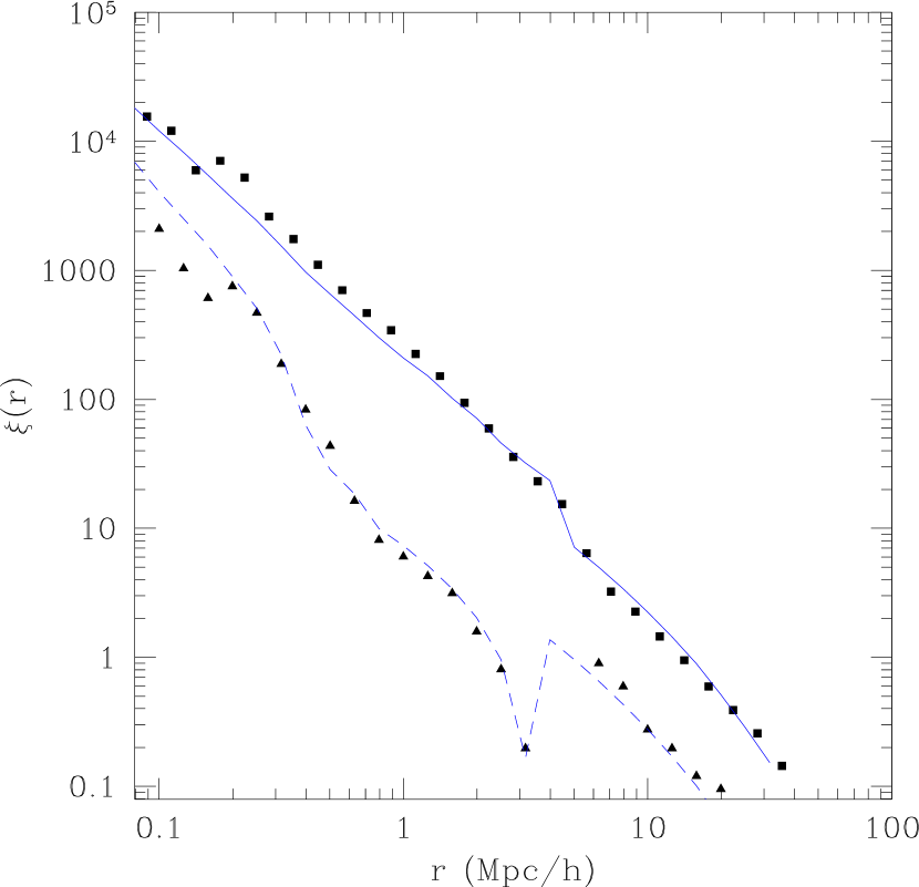
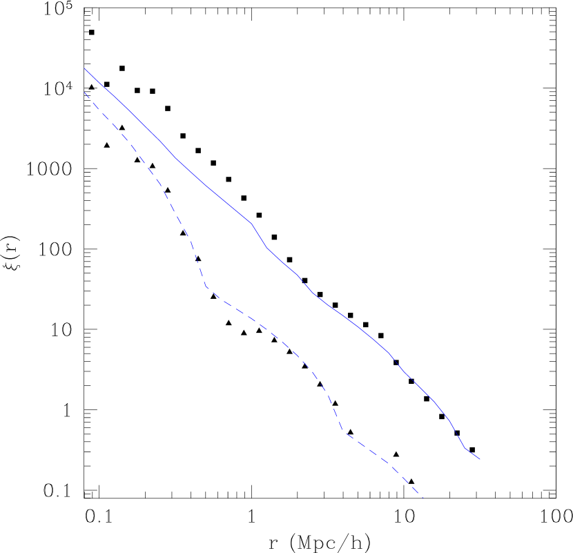
Figure 5: Correlation function for mock galaxies in the VLS simulations. Squares show $\xi(r|\delta)$ for the overdense sample and triangles are for the underdense sample. In the top panel, the density was defined by counting galaxies within spheres having radius $5h^{-1}$Mpc centred on each object, and the bottom panel used $8h^{-1}$Mpc spheres. Curves show the associated analytic model which is able to describe the three different clustering regimes.

However, such a transition is seen in Figure 5, which shows results for a mock galaxy sample in the VLS simulations, constructed with $M_{min}=10^{12.72}h^{-1}M_{\odot}$ and $\alpha=1.39$, chosen to be similar to galaxies more luminous than $M_{r}=-21$. The top and bottom panels show results from analyses in which the large scale environment was defined by the mass within spheres of radii $5h^{-1}$ and $8h^{-1}$Mpc, respectively. The inflection indicating the transition from $\xi_{2h-1p}(r|\delta)$ to $\xi_{2h-2p}(r|\delta)$ is more clearly seen for low density regions, and it is clearer when the scale which defines the environment is smaller. For these more luminous galaxies, using the simpler equation (19) in $P_{2h-1p}$ is an excellent approximation in dense regions, but grossly overestimates (by at least a factor of two) the clustering strength on intermediate scales in underdense regions. In underdense regions, equations (16)–(18) are substantially more accurate. We would like to point out that the relation between $N$ and $M$ (that was mentioned in the previos section) within spheres of $8h^{-1}$Mpc, shows more scatter at large $N$. As the model is more sensitive to larger scatter at large $N$, we believe this causes the analytical prediction to depart from the simulation results at small scales, as shown in the lower panel of Figure 5.

Figure 1 indicates that our model for the environmental dependence of dark matter clustering is accurate, and the agreement between the symbols and the curves in Figures 3 and 5 indicates that our approximate model for the environmental dependence of galaxy clustering also works quite well. Although it is reassuring that the model works so well—it suggests that we understand the physics which drives the environmental dependence of clustering—this analytic description is not needed to perform the test of environmental effects described in the main text.

A.4 Consistency checks

This section shows that the expressions in Section A.2 do reduce to the standard expressions in Section A.1 upon averaging over all environments.

The mass density is

$$\begin{split}\bar{\rho}_{\delta}&=\int_{M_{min}}^{M_{max}}dM\,n(M,V)\int_{0}^{M}dm\,N(m|M,V)\,m\\ &\to\int_{0}^{\infty}dm\,m\int_{m}^{\infty}dM\,n(M,V)\,N(m|M,V)\\ &=\int_{0}^{\infty}dm\,{dn(m)\over dm}\,m\int_{m}^{\infty}dM\,f(M,V|m)\\ &=\int_{0}^{\infty}dm\,{dn(m)\over dm}\,m=\bar{\rho}\end{split}$$ (23)

when $M_{min}\to 0$ and $M_{max}\to\infty$ (this limit corresponds to averaging over all environments). In this limit, the one-halo term is

$$P_{1h}(k|\delta) \to \int_{0}^{\infty}dM\,n(M,V)$$ (24)

$$\quad\times\quad\int_{0}^{M}dm\,N(m|M,V)\left({m\over\bar{\rho}}\right)^{2}|u(k|m)|^{2}$$

$$= \int_{0}^{\infty}dm\,\left({m\over\bar{\rho}}\right)^{2}\,|u(k|m)|^{2}$$

$$\qquad\times\quad\int_{m}^{\infty}dM\,n(M,V)\,N(m|M,V)$$

$$= \int_{0}^{\infty}dm\,{dn(m)\over dm}\,\left({m\over\bar{\rho}}\right)^{2}\,|u(k|m)|^{2}.$$

Similarly, the two halo term becomes

$${P_{2h-2p}(k|\delta)\over P_{Lin}(k|R_{p})} \to \Biggl{[}\int_{0}^{\infty}dM\,n(M,V)\,B(M,V)$$ (25)

$$\times\int_{0}^{M}dm\,N(m|M,V)\left({m\over\bar{\rho}}\right)\,u(k|m)\Biggr{]}^{2}$$

$$= \Biggl{[}\int_{0}^{\infty}dm\,{m\over\bar{\rho}}\,u(k|m)\int_{m}^{\infty}dM\,N(m|M,V)$$

$$\qquad\qquad\times\quad n(M,V)\,B(M,V)\Biggr{]}^{2}.$$

This can be simplified as follows. The halo overdensity is

$$\delta_{h}(m|M,V)={dN(m|M,V)/dm\over V\,dn(m)/dm}-1\equiv b(m|M,V)\,\delta.$$ (26)

When $V\gg 1$, then $\delta\ll 1$, and $M$ is almost surely much larger than the typical halo mass, so $M\gg m$ for most values of $m$. In this limit,

$$\begin{split}{dN(m,\delta_{c}|M,V)/dm\over V\,dn(m)/dm}&=(1+\delta)\,{dn[m,\delta_{c}-\delta_{0}(\delta)]/dm\over dn(m)/dm}\\ \ &\to(1+\delta)\,\left(1-\delta_{0}(\delta){d\ln dn(m)/dm\over d\delta_{c}}\right)\\ \ &\to 1+\delta-\delta\,{d\ln dn(m)/dm\over d\delta_{c}},\end{split}$$ (27)

where we have used the fact that $\delta_{0}\approx\delta\ll 1$. Hence, we can approximate $\delta_{h}(m)\approx b(m)\delta$ where $b(m)\approx 1-d\ln n(m,\delta_{c})/d\delta_{c}$ (equation 2) is no longer a function of $V$. Our assumption is that $B(M)$ is related to $n(M,V)$ similarly. Thus, the second integral in the expression above becomes

$$\int_{m}^{\infty}dM\,n(M,V)\,B(M,V)\,N(m|M,V)$$ (28)

$$= \int_{m}^{\infty}dM\,n(M,V)\,\left[1-{d\ln n(M,V)\over d\delta_{0}}\right]\,N(m|M,V)$$

$$= {dn(m)\over dm}-\int_{m}^{\infty}dM\,{dn(M,V)\over d\delta_{0}}\,N(m|M,V)$$

$$= {dn(m)\over dm}-{d\over d\delta_{0}}\int_{m}^{\infty}dM\,n(M,V)\,N(m|M,V)$$

$$\qquad+\int_{m}^{\infty}dM\,n(M,V)\,{dN(m|M,V)\over d\delta_{0}}$$

$$= {dn(m)\over dm}-{dn(m)\over d\delta_{0}}-{d\over d\delta_{c}}\int_{m}^{\infty}dM\,n(M,V)\,N(m|M,V)$$

$$= {dn(m)\over dm}\left[1-{d\ln dn(m)/dm\over d\delta_{c}}\right]$$

$$= {dn(m)\over dm}\,b(m).$$

Hence

$${P_{2h-2p}(k|\delta)\over P_{Lin}(k|R_{p})}\to\Biggl{[}\int_{0}^{\infty}dm\,{dn(m)\over dm}\,{m\over\bar{\rho}}\,b(m)\,u(k|m)\Biggr{]}^{2}.$$ (29)

If we do not truncate the two-halo term on small scales, as a crude approximation for $P_{2h-1p}$, i.e., if we simply set $P_{Lin}(k|R_{p})\to P_{Lin}(k)$, then this agrees with equation (9).

If we do truncate, then we must check if the large-scale limit of $P_{2h-1p}+P_{2h-2p}$ agrees with equation (9). In the limit of large patches and all environments, the two-halo one-patch term becomes

$${P_{2h-1p}(k|\delta)\over P_{\rm Lin}(k)-P_{\rm Lin}(k|R_{p})}\to\int_{0}^{\infty}dM\,{n(M,V)(1+\delta)\over M/\bar{\rho}}$$

$$\times\left[\int_{0}^{M}dm\,{dn(m)\over dm}\,{m\over\bar{\rho}}\,b(m)\,u(k|m)\,V[1+b(m)\delta]\right]^{2}.$$

On large scales $\delta\ll 1$ so we can ignore $b\delta$ compared to unity. Since $M/\bar{\rho}=V(1+\delta)$,

$${P_{2h-1p}(k|\delta)\over P_{\rm Lin}(k)-P_{\rm Lin}(k|R_{p})}\approx\int_{0}^{\infty}dM\,Vn(M,V)$$

$$\qquad\qquad\qquad\qquad\times\left[\int_{0}^{M}dm\,{dn(m)\over dm}\,\frac{m}{\bar{\rho}}\,b(m)\,u(k|m)\right]^{2}$$

$$\qquad\qquad\approx\int_{0}^{\infty}dM\,Vn(M,V)$$

$$\qquad\qquad\qquad\qquad\times\left[\int_{0}^{\infty}dm\,{dn(m)\over dm}\,\frac{m}{\bar{\rho}}\,b(m)\,u(k|m)\right]^{2}$$

$$\qquad\qquad=\left[\int_{0}^{\infty}dm\,{dn(m)\over dm}\,\frac{m}{\bar{\rho}}\,b(m)\,u(k|m)\right]^{2}$$ (30)

where the second line follows from the fact that if $M$ is much larger than the mass of the largest halo, then the upper limit of the integrals over $m$ can safely be changed from $M$ to $\infty$, and the final line uses the fact that the integral over $M$ which remains is the same as the integral over the counts-in-cells probability distribution, and so equals unity. This shows explicitly that, in this limit, $P_{2h-1p}+P_{2h-2p}$ agrees with equation (9).

References

- Balogh & Morris (2000) Balogh M.L., Morris S.L., 2000, MNRAS, 318, 703
- Balogh et al. (2002) Balogh M.L. et al., 2002, MNRAS, 337, 256
- Balogh et al. (2004) Balogh M.L. et al., 2004, MNRAS, 348, 1355
- Benson et al. (2001) Benson A.J. et al., 2001, MNRAS, 327, 1041
- Blanton et al. (2004) Blanton M.R., Eisenstein D.J., Hogg D.W., Zehavi I., 2004, astro-ph/0411037
- Cole et al. (2000) Cole S., Lacey C.G., Baugh C.M., Frenk C.S., 2000, MNRAS, 319, 168
- Cooray & Sheth (2002) Cooray A., Sheth R.K., 2002, Phys. Rep., 372, 1
- Dressler (1980) Dressler A., 1980, ApJ, 236, 351
- Farouki & Shapiro (1980) Farouki R., Shapiro S.L., 1980, ApJ, 241, 928
- Gao, Springel & White (2005) Gao L., Springel V., White S. D. M., 2005, MNRAS, submitted
- Gomez et al. (2003) Gomez P.L. et al., 2003, ApJ, 584, 210
- Gunn & Gott (1972) Gunn J.E., Gott J.R.I., 1972, ApJ, 528, 118
- Hogg et al (2004) Hogg D.W. et al., 2004, ApJ, 601, L29
- Kaiser (1984) Kaiser N., 1984, ApJ, 284, 9
- Kauffmann et al. (1997) Kauffmann G., Nusser A., Steinmetz M., 1997, MNRAS, 286, 795
- Kauffmann et al. (1999) Kauffmann G., Colberg J.M., Diaferio A., White S.D.M., 1999, MNRAS, 307, 529
- Kauffmann et al. (2004) Kauffmann G. et al., 2004, MNRAS, 353, 713
- Kravtsov et al. (2004) Kravtsov A. et al., 2004, ApJ, 609, 35
- Lacey & Cole (1993) Lacey C., Cole S., 1993, MNRAS, 262, 627
- Lemson & Kauffmann (1999) Lemson G., Kauffmann G., 1999, MNRAS, 302, 111
- Mo & White (1996) Mo H.J., White S.D.M., 1996, MNRAS, 282, 347
- Mo et al. (2004) Mo H. J., Yang X., van den Bosch F. C., Jing Y. P., 2004, MNRAS, 349, 205
- Moore et al. (1996) Moore B., Katz N., Lake G., Dressler A., Oemler A., 1996, Nat, 379, 613
- Navarro et al. (1997) Navarro J.F., Frenk C.S., White S.D.M., 1997, ApJ, 490, 493
- Peebles (1974) Peebles P.J.E., 1974, ApJ, 189, L51
- Peebles (1980) Peebles P.J.E., 1980, The Large-Scale Structure of the Universe. Princeton Univ. Press, Princeton, NJ
- Press & Schechter (1974) Press W.H., Schechter P., ApJ, 1974, 187, 425
- Sheth (1998) Sheth R.K., 1998, MNRAS, 300, 105
- Sheth & Jain (1997) Sheth R.K., Jain B., 1997, MNRAS, 285, 231
- Sheth & Jain (2003) Sheth R.K., Jain B., 2003, MNRAS, 345, 62
- Sheth & Lemson (1999) Sheth R.K., Lemson G., 1999, MNRAS, 304, 767
- Sheth & Tormen (1999) Sheth R.K., Tormen G., 1999, MNRAS, 308, 119
- Sheth & Tormen (2002) Sheth R.K., Tormen G., 2002, MNRAS, 329, 61
- Sheth & Tormen (2004) Sheth R.K., Tormen G., 2004, MNRAS, 350, 1385
- Sheth, Abbas & Skibba (2004) Sheth R.K., Abbas U., Skibba R.A., in Diaferio A., ed, 2004, Proc. IAU Coll. 195, Outskirts of galaxy clusters: intense life in the suburbs, CUP, Cambridge, p. 349
- Sheth et al. 2001 (2001) Sheth R.K., Mo H., Tormen G., 2001, MNRAS, 323, 1
- Sheth et al. (2001) Sheth R.K., Hui L., Diaferio A., Scoccimarro R., 2001, MNRAS, 325, 1288
- Somerville & Primack (1999) Somerville R., Primack J.R.S., 1999, MNRAS, 310, 1087
- White & Frenk (1991) White S.D.M., Frenk C.S., 1991, ApJ, 379, 52
- White & Rees (1978) White S.D.M., Rees M.J., 1978, MNRAS, 183, 341
- Yang et al. (2003) Yang X., Mo H.J., van den Bosch F.C., 2003, MNRAS, 339, 1057
- Zehavi et al. (2004) Zehavi I. et al., 2004, astro-ph/0408569