Oscillations of rotating bodies: A self-adjoint formalism applied to dynamic tides and tidal capture

Abstract

We consider the excitation of the inertial modes of a uniformly rotating fully convective body due to a close encounter with another object. This could lead to a tidal capture or orbital circularisation depending on whether the initial orbit is unbound or highly eccentric. We develop a general self-adjoint formalism for the response problem and thus solve it taking into account the inertial modes with $m=2$ for a full polytrope with $n=1.5.$ We are accordingly able to show in this case that the excitation of inertial modes dominates the response for large impact parameters and thus cannot be neglected in calculations of tidal energy and angular momentum exchange or orbital circularisation from large eccentricity.

1 Introduction

The process of tidal capture of a body into a bound orbit through the excitation of oscillatory internal modes is thought to be of general importance in astrophysics. It is likely to play a role in binary formation in globular clusters (eg. Press & Teukolsky, 1977, hereafter PT and references therein) as well as in tidal interactions of stars within galactic centres. When there are repeated close encounters as for a highly eccentric orbit, circularisation may result, a process of potential importance for extrasolar planets (eg. Ivanov & Papaloizou 2004, hereafter IP).

Until now, only the oscillation modes associated with spherical non rotating stars have been considered with possibly rotation being treated as a perturbation (eg. PT,IP). But angular momentum is transfered in tidal encounters and when, as is often the case, the internal inertia is much less than that of the orbit, the tidally excited object would be expected to rotate at a balanced rate or undergo pseudo synchronisation. Then the rotation frequency is matched to the most important ones in a Fourier decomposition of the tidal forcing. It is then natural to expect that inertial modes controlled by the rotation (see eg. Papaloizou & Pringle 1981, hereafter PP) become important for the tidal response. This is especially the case for a barotropic configuration , with no stratification and hence no low frequency $g$ modes. We would expect inertial modes, which have periods that scale with the rotation frequency, to be particularly important for large periastron distances as the fundamental spherical modes suffer increasing frequency mismatch as this distance increases.

It is the purpose of this paper to calculate the response of a rotating body taking the inertial modes into account. In particular we focus on modes with $m=2$ which dominate the angular momentum exchange and a full polytrope with index $n=1.5.$ We show that the inertial modes indeed dominate the response at larger periastron distances of interest in many cases.

In section 2 we give the basic equations governing the linear response of a uniformly rotating barotropic star to the tidal forcing due to a close encounter. In section 3 we give a self-adjoint representation of the linear problem and discuss how it can be used to provide a formal solution in terms of a spectral decomposition as can be done for a non rotating star. In section 4 we develop expressions for the energy and angular momentum exchange. In section 5 we give results for a polytrope with index $n=1.5$, showing that the $m=2$ inertial wave response is contained within just a few global modes and that inertial modes dominate the tidal response for large periastron passages. Accordingly these must be considered when discussing tidal circularisation from large eccentricity for objects such as extrasolar planets.

2 Basic equations

We assume that the star is rotating with uniform angular velocity ${\Omega}$ directed perpendicular to the orbital plane. In this case the hydrodynamic equations for the perturbed quantities take the simplest form in the rotating frame. For a convective star, approximated as barotropic, we have

$${D^{2}{\mbox{\boldmath${\xi}$}}\over Dt^{2}}+2{\mbox{\boldmath${\Omega}$}}\times{D\mbox{\boldmath${\xi}$}\over Dt}=-\nabla W.$$ (1)

Here ${\xi}$ is the Lagrangian displacement vector, and

$$W=c_{s}^{2}\rho^{{}^{\prime}}/\rho+\Psi^{int}+\Psi^{ext},$$ (2)

where $\rho$ is the density, $\rho^{{}^{\prime}}$ is the density perturbation, $c_{s}$ is the adiabatic sound speed, $\Psi^{int}$ is the stellar gravitational potential arising from the perturbations and $\Psi^{ext}$ is the external forcing tidal potential. Note that the centrifugal term is absent in equation $(\ref{eq 1})$ being formally incorporated into the potential governing the static equilibrium of the unperturbed star. The convective derivative ${D\over Dt}\equiv{\partial\over\partial t}$ as there is no unperturbed motion in the rotating frame.

The linearised continuity and Poisson equations are

$$\rho^{{}^{\prime}}=-\nabla(\rho{\mbox{\boldmath${\xi}$}})\quad{\rm and}\quad\Delta\Psi^{int}=4\pi G\rho^{{}^{\prime}}.$$ (3)

We use a cylindrical coordinate system $(\varpi,\phi,z)$ with origin at the centre of the star and assume that the tidal potential and the resulting perturbation to some quantity, say $Q$, is represented in terms of a Fourier transform over the angle $\phi$ and time $t$. Thus $Q=\sum_{m}\left(\exp({im\phi})\int^{+\infty}_{-\infty}d\sigma\tilde{Q}_{m}\exp({-i\sigma t})+cc\right)$, where the sum is over $m=0$ and $2$ and $cc$ denotes the complex conjugate. The reality of $Q$ implies that the Fourier transform, indicated by tilde satisfies $\tilde{Q}_{m}(\sigma)=\tilde{Q}_{-m}^{*}(-\sigma).$

To solve the forcing problem we obtain equations for the Fourier transforms of the perturbations using $(\ref{eq 1})-(\ref{eq 3}).$ We can then express $\tilde{\mbox{\boldmath${\xi}$}}_{m}$ in terms of $\tilde{W}_{m}$ with help of $(\ref{eq 1})$, the density perturbation in terms of $\tilde{\Psi}^{ext}_{m}$, $\tilde{\Psi}^{int}_{m}$ and $\tilde{W}_{m}$ with help of (2), and substitute the results into the continuity equation (3) to get

$$\sigma^{2}{\mbox{\boldmath${A}$}}\tilde{W}_{m}-\sigma{\mbox{\boldmath${B}$}}\tilde{W}_{m}-{\mbox{\boldmath${C}$}}\tilde{W}_{m}=\sigma^{2}d{\rho\over c_{s}^{2}}(\tilde{\Psi}^{ext}_{m}+\tilde{\Psi}^{int}_{m}-\tilde{W}_{m}),$$ (4)

where $d=4\Omega^{2}-\sigma^{2}$, and

$${\mbox{\boldmath${A}$}}=-{1\over\varpi}{\partial\over\partial\varpi}\left(\varpi\rho{\partial\over\partial\varpi}\right)-{\partial\over\partial z}\left(\rho{\partial\over\partial z}\right)+{m^{2}\rho\over\varpi^{2}},$$ (5)

$${\mbox{\boldmath${B}$}}=-{2m\Omega\over\varpi}{\partial\rho\over\partial\varpi},\quad{\mbox{\boldmath${C}$}}=-4\Omega^{2}{\partial\over\partial z}\left(\rho{\partial\over\partial z}\right).$$ (6)

It is very important to note that the operators ${A}$, ${B}$ and ${C}$ are self-adjoint when the inner product

$$(W_{1}|W_{2})=\int_{V}dz\varpi d\varpi W^{*}_{1}W_{2},$$ (7)

with $V$ denoting the volume of the star. Also when $W$ is not a constant ${A}$ and ${B}$ are positive definite and ${C}$ is non negative definite. Equations (2), (4) and the Poisson equation (3) form a complete set.

When $\tilde{\Psi}^{ext}_{m}=0,$ equation (4) describes the free oscillations of a rotating star. These may be classified as relatively high frequency $f$ and $p$ modes and inertial modes with eigen frequencies $\sigma\sim\Omega$. The $f$ and $p$ modes exist in non rotating stars and can be treated in a framework of perturbation theory (eg. IP). Here we focus on the response of inertial waves to tidal forcing, for slow rotation. We seek a solution as a series expansion in the small parameters $\sigma/\Omega_{*}$ and $\Omega/\Omega_{*}$, where $\Omega_{*}=\sqrt{(GM_{*}/R^{3}_{*})}$, with $M_{*}$ and $R_{*}$ being the mass and the radius of the star, respectively. The small parameters will be assumed to be of the same order.

To zeroth order (when $\sigma\rightarrow 0$) the tidal potential induces a quasi-static bulge in which tidal forces are balanced by pressure and self gravity and $\tilde{\rho}^{{}^{\prime}}_{m}\rightarrow\tilde{\rho}_{m,st}$ with ${\tilde{\Psi}^{int}_{m}}\rightarrow{\tilde{\Psi}^{int}_{m,st}}$. From equation (4) we conclude that $W$ is smaller than the potential perturbations by a factor of order $\sigma^{2}/\Omega^{2}_{*}$ (see PP for details). Accordingly, setting $W=0$ in equation (2) and using equation (3) we obtain

$$\tilde{\rho}_{m,st}=-{\rho\over c^{2}_{s}}(\tilde{\Psi}^{int}_{m,st}+\tilde{\Psi}^{ext}),\quad\Delta\Psi^{int}_{m,st}=4\pi G\tilde{\rho}_{m,st}.$$ (8)

In the lowest order approximation we find $\tilde{W}_{m}$ using equation (4) neglecting the higher order term proportional to $\rho\tilde{W}_{m}/c_{s}^{2}$ on the right hand side. We thus have

$$\sigma^{2}{\mbox{\boldmath${A}$}}\tilde{W}_{m}-\sigma{\mbox{\boldmath${B}$}}\tilde{W}_{m}-{\mbox{\boldmath${C}$}}\tilde{W}_{m}=S,$$ (9)

where the source term

$$S=-\sigma^{2}d\tilde{\rho}_{m,st}=\sigma^{2}d{\rho\over c_{s}^{2}}(\tilde{\Psi}^{ext}_{m}+\tilde{\Psi}^{int}_{m,st})$$ (10)

is completely determined by the external forcing via equation (8). Finally, the perturbation of the internal gravitational potential associated with $\tilde{W}_{m}$, $\delta\tilde{\Psi}_{m}=\tilde{\Psi}^{int}_{m}-\tilde{\Psi}^{int}_{m,st}$ follows from (2), (3) and (8)

$$\Delta\delta\tilde{\Psi}_{m}={4\pi G\rho\over c_{s}^{2}}(\tilde{W}_{m}-\delta\tilde{\Psi}_{m}).$$ (11)

3 Reduction of the problem to standard self-adjoint form and formal solution

Equation (9) is of a general type that governs the linear response of rotating bodies in a context that is much wider than the specific one considered here ( see Lynden Bell & Ostriker 1967). One recurring difficulty has been that the way in which the frequency $\sigma$ occurs does not readily allow application of the general spectral theory of self-adjoint operators to the response calculation even though ${A}$, ${B}$ and ${C}$ are themselves self-adjoint (eg. Dyson & Schutz 1979). We here provide a formulation in which the problem can be dealt with in the same way as a standard self-adjoint one such as occurs for a non rotating star.

We begin by remarking that the self-adjoint and non negative character of ${A}$, ${B}$ and ${C}$ allows the spectral theorem to be used to specify their square roots, eg. ${\mbox{\boldmath${A}$}}^{1/2}$, defined by condition ${\mbox{\boldmath${A}$}}={\mbox{\boldmath${A}$}}^{1/2}{\mbox{\boldmath${A}$}}^{1/2}$. The positiveness of ${A}$ allows definition of the inverse of ${\mbox{\boldmath${A}$}}^{1/2}$, ${\mbox{\boldmath${A}$}}^{-1/2}$. Technically, this is done through using the spectral decomposition

$${\mbox{\boldmath${A}$}}W=\sum_{j}\lambda_{j}\phi_{j}\left<W|\phi_{j}\right>\quad F({\mbox{\boldmath${A}$}})W=\sum_{j}F(\lambda_{j})\phi_{j}\left<W|\phi_{j}\right>,$$ (12)

..etc., where $\phi_{j}$ and $\lambda_{j}$ are the eigenfunctions and the eigenvalues of the corresponding operators and the last equation defines a general function of the operator ${A}$. The sum may formally include integration with an appropriate measure in the case of a continuous spectrum of the corresponding operators.

Now let us consider a generalised two dimensional vector $\vec{Z}$ with components such that $\vec{Z}=(Z_{1},{\mbox{\boldmath${C}$}}^{1/2}\tilde{W}_{m})$ and the straightforward generalisation of the inner product given by equation (7). It is easy to see that equation (9) can be derived from the matrix form

$$\sigma\vec{Z}={\mbox{\boldmath${H}$}}\vec{Z}+\vec{S},$$ (13)

where

$${\mbox{\boldmath${H}$}}=\left(\begin{array}[]{cc}{\mbox{\boldmath${A}$}}^{-1/2}{\mbox{\boldmath${B}$}}{\mbox{\boldmath${A}$}}^{-1/2}&{\mbox{\boldmath${A}$}}^{-1/2}{\mbox{\boldmath${C}$}}^{1/2}\\ {\mbox{\boldmath${C}$}}^{1/2}{\mbox{\boldmath${A}$}}^{-1/2}&0\end{array}\right),$$ (14)

and the source vector $\vec{S}$ has the components $({\mbox{\boldmath${A}$}}^{-1/2}S,0).$ It then follows from (13) that we may choose $Z_{1}=\sigma{\mbox{\boldmath${A}$}}^{1/2}\tilde{W}_{m}.$ Since the off diagonal elements in the matrix (14) are adjoint of each other and the diagonal elements are self adjoint, that the operator ${H}$ is self-adjoint is manifest. Now we can use the spectral theory of self-adjoint operators to look for a solution to (9) in the form $\vec{Z}=\sum_{k}\alpha_{k}\vec{Z}_{k}$, where $\vec{Z}_{k}$ are the real eigenfunctions of ${H}$ which satisfy

$$\sigma_{k}\vec{Z}_{k}={\mbox{\boldmath${H}$}}\vec{Z}_{k},$$ (15)

the associated necessarily real eigen frequencies being $\sigma_{k}.$

Substituting (15) into (13) we obtain

$$\alpha_{k}={<\vec{Z}_{k}|\vec{S}>\over<\vec{Z}_{k}|\vec{Z}_{k}>(\sigma+i\nu-\sigma_{k})},$$ (16)

where, following the Landau prescription, we have added an infinitesimal imaginary part $\nu>0$ to the frequency $\sigma.$ The inner product induced by ${H}$ turns out to be $<\vec{Z}_{k}|\vec{Z}_{l}>=\sigma_{k}\sigma_{l}(W_{k}|{\mbox{\boldmath${A}$}}W_{l})+(W_{k}|{\mbox{\boldmath${C}$}}W_{l})$, where $W_{k}={\mbox{\boldmath${C}$}}^{-1/2}Z_{2}^{k}=\sigma_{k}^{-1}{\mbox{\boldmath${A}$}}^{-1/2}Z_{1}^{k}$. Using (10) and (16) we explicitly obtain

$$\tilde{W}_{m}=\sigma d\sum_{k}{\sigma_{k}^{2}(W_{k}|\tilde{\rho}_{m,st})\over N_{k}(\sigma_{k}-i\nu-\sigma)}W_{k},$$ (17)

where $N_{k}=\sigma^{2}_{k}(W_{k}|{\mbox{\boldmath${A}$}}W_{k})+(W_{k}|{\mbox{\boldmath${C}$}}W_{k})$ is the norm.

4 Transfer of energy and angular momentum from orbit to inertial waves

The time derivative $\dot{E}$ of the wave energy $E$ associated with the rotating frame and the time derivative $\dot{L}$ of the wave angular momentum $L$ are given by usual expressions

$$\dot{E}=-\int d\phi\left(\dot{\rho}^{{}^{\prime}}|\Psi_{ext}\right),\quad\dot{L}=-\int d\phi\left(\rho^{{}^{\prime}}|{\partial\Psi_{ext}\over\partial\phi}\right).$$ (18)

The wave energy associated with the inertial frame, $E_{I}$ is given in terms of $E$ and $L$ (eg. Friedman $\&$ Schutz 1978, hereafter FS) through

$$E_{I}=E+\Omega L.$$ (19)

Expressing $\rho^{{}^{\prime}}$ with help of (2) in terms of $W$ and discarding the total derivatives which cannot contribute to the total energy transfer $\Delta E=\int^{+\infty}_{-\infty}dt\dot{E}$, we obtain

$$\Delta E=-\int^{+\infty}_{-\infty}dt\int^{2\pi}_{0}d\phi\left({\rho\over c^{2}_{s}}(\dot{W}-\delta\dot{\Psi})|\Psi^{ext}\right).$$ (20)

Contributions $\Delta E_{m}$ to $\Delta E$ arising from different values of $m$ may be calculated separately. Substituting the corresponding Fourier transforms into (20), and integrating over time, we obtain

$$\Delta E_{m}=4\pi^{2}i\int d\sigma\sigma\{(\tilde{\Psi}^{ext}_{m}|\delta\tilde{\rho}_{m})-(\delta\tilde{\rho}_{m}|\tilde{\Psi}^{ext}_{m})\},$$ (21)

where $\delta\tilde{\rho}_{m}={\rho\over c^{2}_{s}}(\tilde{W}_{m}-\delta\tilde{\Psi}_{m})$. Note that for the problem on hand $\Psi^{ext}_{m}$ and $\Psi^{int}_{m,st}$ are real (see below). Now we substitute the spectral decomposition $\delta\tilde{\Psi}_{m}=\sum_{k}\alpha_{k}\delta\Psi_{k}$, where $\Delta\delta\Psi_{k}={4\pi G\rho\over c^{2}_{s}}(W_{k}-\delta\Psi_{k})$, together with (17) into (21). The singularities in the integral over $\sigma$ corresponding to $\sigma=\sigma_{k}$ and determining all non-zero contributions to the integral are dealt with using the Landau prescription. Then the energy transfer is a sum of contributions associated with each mode, being given by

$$\Delta E_{m}=-8\pi^{3}\sum_{k}{\sigma_{k}^{4}(4\Omega^{2}-\sigma^{2}_{k})\over N_{k}}(W_{k}|\tilde{\rho}_{m,st})(\delta\rho_{m,k}|\tilde{\Psi}^{ext}_{m}),$$ (22)

where $\delta\rho_{m,k}={\rho\over c_{s}^{2}}(W_{k}-\delta\Psi_{k})$, and both integrals are evaluated for $\sigma=\sigma_{k}$.

Using the symmetry properties of the operator $\Delta+{4\pi G\rho\over c_{s}^{2}}$ one can readily see that the integrals are, in fact, the negatives of each other, thus we finally obtain

$$\Delta E_{m}=8\pi^{3}\sum_{k}{\sigma_{k}^{4}(4\Omega^{2}-\sigma^{2}_{k})\over N_{k}}A^{2}_{k},$$ (23)

where $A_{k}=|(\tilde{\rho}_{m,st}|W_{k})|$.

The expression for the angular momentum transfer follows immediately from (23) and the general relation between wave energy and angular momentum corresponding to a mode with particular value of $m$: $E_{m}/L_{m}=\sigma/m$ (eg. FS). We have $\Delta L_{0}=0$ and

$$\Delta L_{2}=16\pi^{3}\sum_{k}{\sigma_{k}^{3}(4\Omega^{2}-\sigma^{2}_{k})\over N_{k}}A^{2}_{k}.$$ (24)

The expressions (23), (24) can be evaluated when the star is in a parabolic orbit, being the limit of a highly eccentric orbit, using the expression for $\tilde{\Psi}^{ext}$ given in the quadrupole approximation by PT. From this we obtain

$$\tilde{\Psi}^{ext}_{m}=\sqrt{{5\over 2\pi^{3}}{(2-|m|)!\over(2+|m|)!}}{B_{|m|}\over(1+q)}I_{2,-m}(y)\Omega_{p}r^{2}P^{|m|}_{2}(\cos\theta),$$ (25)

where $B_{2}=\sqrt{{3\pi\over 10}}$, $B_{0}=-{1\over 2}\sqrt{{\pi\over 5}}$. $q$ is the ratio of $M_{*}$ to the mass of the star exerting the tides, $M$: $q=M_{*}/M$. $\Omega_{p}=\sqrt{{GM(1+q)\over R^{3}_{p}}}$ is a typical frequency of periastron passage and $R_{p}$ is the periastron distance. The functions $I_{2,-m}(y)$ specify the dependence of $\tilde{\Psi}^{ext}_{m}$ on $\sigma$, they are described by PT. y=$\bar{\Omega}(\bar{\sigma}+m)$, where we use dimensionless frequencies $\bar{\sigma}=\sigma/\Omega$ and $\bar{\Omega}=\Omega/\Omega_{p}$. $P_{l}^{m}(x)$ is the associated Legendre function, and $(r,\theta)$ are the spherical coordinates.

Now we express the density perturbation entering in (23), (24) as $\tilde{\rho}_{m,st}=-{\rho\over c_{s}^{2}}F\tilde{\Psi}^{ext}_{m}.$ Here we introduce a factor $F$ to account for self-gravity of the star that can be obtained from the solution of (8)  . We substitute this expression and (25) in (23), (24) and express all quantities in natural units. These are such that the spatial coordinates, density and sound speed are expressed in units of $R_{*}$, the averaged density ${\bar{\rho}}={3M_{*}\over 4\pi R_{*}^{3}}$, and $\sqrt{GM_{*}\over R_{*}}$, respectively. We then have

$$\Delta E_{m}={C_{m}\over(1+q)^{2}}\bar{\Omega}^{4}\sum_{k}\{\bar{\sigma}_{k}^{4}(4-\bar{\sigma}_{k}^{2})Q_{k}^{2}I^{2}_{2,-m}(y)\}{E_{*}\over\eta^{6}},$$ (26)

$$\Delta L_{2}={2C_{2}\over(1+q)^{2}}\bar{\Omega}^{3}\sum_{k}\{\bar{\sigma}_{k}^{3}(4-\bar{\sigma}_{k}^{2})Q_{k}^{2}I^{2}_{2,-m}(y)\}{L_{*}\over\eta^{5}},$$ (27)

where $E_{*}={GM_{*}\over R_{*}}$, $L_{*}=M_{*}\sqrt{GM_{*}R_{*}}$, and $\eta={\Omega_{*}/\Omega_{p}}=\sqrt{M_{*}R_{p}^{3}\over(1+q)MR_{*}^{3}}$, $C_{2}={3\over 16}$ and $C_{0}=3/4$. The overlap integrals $Q_{k}$ have the form:

$$Q_{k}=({\rho\over c_{s}^{2}}Fr^{2}P^{m}_{2}|W_{k})/\sqrt{\bar{N}_{k}},$$ (28)

where $\bar{N}_{k}=N_{k}/\Omega^{2}$.

5 Numerical Calculations

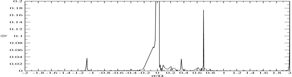
Figure 1: The dependence of $Q_{k}$ on the values of $\sigma_{k}$.

The eigen frequencies $\bar{\sigma}_{k}$ and the integrals $Q_{k}$ in equations (26-27) have to be calculated numerically, for a given model of the star. Therefore, equation (15) describing free oscillations of the star must be solved. For our numerical work we model the star as $n=1.5$ polytrope and use the method of solution of (15) proposed by PP . Namely, we reduce (15) to an ordinary matrix equation using an appropriate set of trial functions, and solve the corresponding eigenvalue problem. The details of our approach will be given in a separate publication. Here we note that we use different numbers $N_{t}$ of the trial functions to study convergence of our numerical scheme with the largest number being equal to $N^{max}_{t}=225$. Also we adopt a spherical model of the star assuming that the distortion of the stellar structure due to rotation does not influence significantly our results. Since the modes corresponding to $m=2$ fully determine the transfer of angular momentum in the quadrupole approximation and apparently dominate the energy transfer, which can only be increased if $m=0$ modes are included, we consider only them.

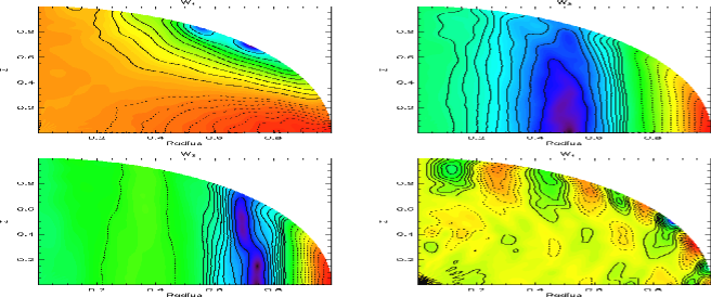
Figure 2: The distribution of $\tilde{W}_{k}$ over the star. $\tilde{W}_{k}=0$ at the origin. Contour lines of different style correspond to values of $\tilde{W}_{k}$ of opposite signs. The upper left (right) plot corresponds to $\sigma_{1}=-1.063$ ( $\sigma_{2}=0.697$). The lower left (right) plot corresponds to $\sigma_{3}=0.362$ ($\sigma_{4}=0.703$).

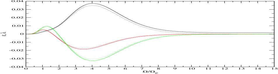
Figure 3: The dependence of the dimensionless quantities $\epsilon$, $\epsilon_{I}$ and $\lambda$ on $\bar{\Omega}$ (see (29) and the text for definitions).

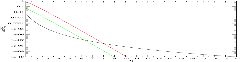
Figure 4: The dependence of the energy transfer on $\eta$. The black curve (red and green) give the contribution of the inertial waves (fundamental mode). We assume that $q\ll 1$ and $\bar{\Omega}=\bar{\Omega}_{crit}\approx 1.6$.

The absolute values of the eigen frequencies $\sigma_{k}$ are always smaller than or equal to $2\Omega$. For complete polytropes it is expected that they ultimately yield an everywhere dense discrete spectrum (PP). In our numerical approach their number is equal to $2N_{t}$, and therefore the number of the terms in the series in (26) and (27) depends on $N_{t}$. However, only the eigenfunctions with some definite values of $\sigma_{k}$ give a significant contribution to the series. These terms correspond to global eigen modes with a large scale distribution of $\tilde{W}_{k}$ over the star. Therefore, the overlap integrals corresponding to the global modes are not averaged to small values after integration over the volume of the star. The number of the global modes does not depend on $N_{t}$. In figure 1 we show the overlap integrals as functions of the eigen frequencies. There is a sharp rise of $Q_{k}$ near $\sigma_{k}=0$ and very close to $\sigma_{k}=2$, and several peaks corresponding to different values of $\sigma_{k}$. The rise at $\sigma_{k}\approx 0$, $2$ is due to numerical inaccuracy of our method, but the corresponding modes practically do not influence our results and therefore the numerical inaccuracy is not significant for our purposes. Note that the feature at $\sigma_{k}\approx 0$ can be removed by an appropriate regularisation of ${C}$.

Three peaks with $\sigma_{1}=-1.063$ and $Q_{1}=0.037$, $\sigma_{2}=0.697$ and $Q_{2}=0.175$, $\sigma_{3}=0.362$ and $Q_{3}=0.034$ correspond to the global modes. The spatial distribution of the corresponding eigenfunctions is shown in figure 2. For comparison we also show a non global mode with $\sigma_{4}=0.703$ and a very small value of $Q_{4}$. It is clear from this figure that the global modes have a large scale distribution of $\tilde{W}_{k}$.

It follows from (26) and (27) that for a given model of the star, the quantities

$$\epsilon_{m}=(1+q)^{2}\eta^{6}(\Delta E_{m}/E_{*}),\quad\lambda=(1+q)^{2}\eta^{5}(\Delta L_{2}/L_{*}),$$ (29)

depend only on $\bar{\Omega}$. In figure 3 we show the dependence of $\epsilon_{2}$ (the solid black curve) and $\lambda$ (the solid red curve) on $\bar{\Omega}$. The solid green curve shows the dependence of the energy transfer in the inertial frame, $\epsilon_{I}=\epsilon_{2}+\bar{\Omega}\lambda$. Note that the energy transfer in the inertial frame is negative when $\bar{\Omega}>2$. The dotted curves show the dependencies of the corresponding quantities calculated with only two global modes, the retrograde mode with $\sigma_{1}=-1.063$ and the prograde mode with $\sigma_{2}=0.697$. Figure 3 shows that the dotted and the solid curves are very close to each other. Therefore, only two modes are essential for our problem. The angular momentum transfer is equal to zero when $\bar{\Omega}=\bar{\Omega}_{crit}=1.6$, where $\epsilon_{crit}\approx 0.0065$. The condition $\Delta L_{2}=0$ may be easily realised in an astrophysical situation where the inertial modes dominate the tidal response and the moment of inertia of the star is sufficiently small. In this case the system quickly relaxes to the so-called state of pseudo synchronisation where $\Delta L_{2}=0$. In figure 4 we show the dependence of $\Delta E/E_{*}$ on $\eta$ for this case. The black curve shows the contribution of the inertial waves,

$$\Delta E_{2}\approx{0.0065\over(1+q)^{2}\eta^{6}}E_{*}.$$ (30)

The red curve shows the contribution of the $f$ mode to the energy transfer calculated for a non-rotating star (PT) and the green curve shows the same quantity but calculated when $\bar{\Omega}=\bar{\Omega}_{crit}$ (IP) . It is clear from this figure that when $\eta>8$ the inertial waves dominate the tidal response. For a planet with Jupiter mass and radius circularising from large eccentricity to attain a final period of $6$ days, $\eta\sim 18$ (IP), such that inertial modes dominate by a wide margin.

6 Conclusions

In this Paper we formulate a new self-adjoint approach to the problem of oscillations of uniformly rotating fully convective star and apply this approach to the tidal excitation of the inertial waves and tidal capture. The approach can be used in any other problem where oscillations with typical frequencies of the order of the angular velocity are important. It can also be extended to the case of convectively stable stars. The oscillations with higher frequencies can also be treated in framework of an extension of our formalism.

We show that the tidal response due to inertial waves can be represented as a spectral decomposition over normal modes. This formalism is general enough to be applied even when the spectrum is not regular and discrete. For full polytropes, only a few global modes with a large scale distribution of the perturbed quantities over the star contribute significantly to the response. We find general expressions for the energy and angular momentum transfer between the orbit and inertial waves. It is shown that when the inertial waves dominate the tidal response and a state of pseudo synchronisation is reached the energy transfer is determined by simple equation (30). As follows from that equation the energy transfer does not decrease exponentially with the orbital periastron and therefore at large periastra the energy transfer due to inertial waves dominates over the energy transfer due to excitation of the fundamental mode. This can be very important for the problem of tidal circularisation of the extra solar planets (see above, IP and references therein), and can be of interest for other problems, such as eg. the problem of tidal capture of convective stars in globular clusters. The application of our approach to extra solar planets will be discussed in a separate publication.

References

- (1) Dintrans, B., Ouyed, R., 2001, AA, 375, L47
- (2) Dyson, J., Schutz, B. F., 1979, RSPSA, 368, 389
- (3) Friedman, J. L., Schutz, B. F., 1978, ApJ, 221, 937 (FS)
- (4) Ivanov, P., Papaloizou, J., 2004, MNRAS, 347, 437 (IP)
- (5) Lockitch, K. H., Friedman, J. L., 1999, ApJ, 521, 764
- (6) Lynden Bell D., Ostriker, J. P., 1967, MNRAS, 136, 293
- (7) Papaloizou, J., Pringle, J. E., 1981, MNRAS, 195, 743 (PP)
- (8) Press, W. H., Teukolsky, S. A., 1977, ApJ, 213, 183 (PT)