$T\rm_{eff}$ and $\log g$ Determinations

Abstract

A discussion on the determination of effective temperature ($T\rm_{eff}$) and surface gravity ($\log g$) is presented. The observational requirements for model-independent fundamental parameters are summarized, including an assessment of the accuracy of these values for the Sun and Vega. The use of various model-dependent techniques for determining $T\rm_{eff}$ and $\log g$ are outlined, including photometry, flux fitting, and spectral line ratios. A combination of several of these techniques allows for the assessment of the quality of our parameter determinations. While some techniques can give precise parameter determinations, the overall accuracy of the values is significantly less and sometimes difficult to quantify.

1 Introduction

The stellar atmospheric parameters of effective temperature ($T\rm_{eff}$) and surface gravity ($\log g$) are of fundamental astrophysical importance. They are the prerequisites to any detailed abundance analysis. As well as defining the physical conditions in the stellar atmosphere, the atmospheric parameters are directly related to the physical properties of the star; mass ($M$), radius ($R$) and luminosity ($L$).

Model atmospheres are our analytical link between the physical properties of the star ($M$, $R$ and $L$) and the observed flux distribution and spectral line profiles. These observations can be used to obtain values for the atmospheric parameters, assuming of course that the models used are adequate and appropriate. The values of $T\rm_{eff}$ and $\log g$ obtained must necessarily be consistent with the actual values of $M$, $R$ and $L$. Unfortunately, the physical properties of stars are not generally directly ascertainable, except in the cases of a few bright stars and certain binary systems. We have to rely on model atmosphere analyses of spectra in order to deduce the atmospheric parameters.

We need to be confident in the atmospheric parameters before we start any detailed analyses. This is especially important when comparing stars with peculiar abundances to normal ones.

1.1 Effective Temperature

The effective temperature of a star is physically related to the total radiant power per unit area at stellar surface ($F\rm_{\ast}$):

$$\sigma\mbox{$T\rm_{eff}$}^{4}\equiv\ \int_{0}^{\infty}F_{\nu}d\nu=\mbox{$F\rm_{\ast}$}=\frac{L}{4\pi R^{2}}$$

It is the temperature of an equivalent black body that gives the same total power per unit area, and is directly given by stellar luminosity and radius.

Since there is not true ‘surface’ to a star, the stellar radius can vary with the wavelength of observation and nature of the star. Radius is taken as the depth of formation of the continuum, which in the visible region is approximately constant for most stars (Gray, 1992).

Providing there is no interstellar reddening (or due allowance for it is made), the the total observed flux at the earth ($f\rm_{\oplus}$) can be used to determine the total flux at the star:

$$\mbox{$F\rm_{\ast}$}=\frac{\theta^{2}}{4}\mbox{$f\rm_{\oplus}$}$$

The only additional requirement is a determination of the stellar angular diameter ($\theta$). This can be obtained directly using techniques such as speckle photometry, interferometry, and lunar occultations, and indirectly from eclipsing binary systems with known distances. We must, however, be aware that some of these methods require the (not always explicit) use of limb-darkening corrections.

1.2 Surface Gravity

The surface gravity of a star is directly given by the stellar mass and radius:

$$g=g_{\odot}\frac{M}{R^{2}}$$

or, logarithmically,

$$\log g=\log M-2\log R+4.437$$

Surface gravity is a measure of the photospheric pressure of the stellar atmosphere. Direct measurements are possible from eclipsing spectroscopic binaries, but again be aware of hidden model atmosphere dependences.

2 Fundamental Stars

A fundamental star has at least one of its atmospheric parameters obtained without reference to model atmospheres. An ideal fundamental star will have both parameters measured. These stars are vital for the quality assurance of model predictions. Unfortunately, the number of fundamental stars is relatively limited by the lack of suitable measurements. There now follows a non-exhaustive summary of the main sources of observational data.

2.1 Sources of Stellar Fluxes

Ultraviolet fluxes have been obtained by various space-based observatories: TD1 (Thompson et al., 1978; Jamar et al., 1976; Macau-Hercot et al., 1978), OAO-2 (Code et al., 1980), and the IUE final archive. HST is also another potential source of flux-calibrated ultraviolet spectra.

Optical spectrophotometry can be obtained various sources, such as Breger (1976); Adelman et al. (1989); Burnashev (1985); Glushneva et al. (1998). The ASTRA spectrophotometer should soon provide a large amount of high-precision stellar flux measurements (Adelman et al., 2005). In the absence of suitable spectrophotometry, optical fluxes can be estimated from photometry (Smalley & Dworetsky, 1995; Smalley et al., 2002).

Infrared flux points can be obtained from the 2MASS, DENIS and IRAS surveys, as well as the compilation by Gezari et al. (1999).

2.2 Sources of Angular Diameters

Useful catalogues of angular diameter measurements are CADARS (Pasinetti-Fracassini et al., 2001) and CHARM2 (Richichi et al., 2005). But, beware, not all are direct measurements!

Incidentally, Kervella et al. (2004a) have produced a good surface brightness relationship for main-sequence and sub-giants. While it is obviously not for use of fundamental parameters, it can be used in the determination of stellar distances (See for example Southworth et al. 2005).

2.3 Source of Masses and Radii

Detached eclipsing binary systems are our source of stellar masses and radii. These are often accurate to 1$\sim$2%, and give us our direct $\log g$ determinations. Useful sources include Popper (1980), Andersen (1991), Perevozkina & Svechnikov (1999), Lastennet & Valls-Gabaud (2002).

For use in $T\rm_{eff}$ determinations, radii need to be converted into angular diameters, which requires an accurate distance determination. For example, the HIPPARCOS parallax catalogue (ESA, 1997), or the membership of a cluster with a known distance, provided that distance has not been obtained using model-dependent methods.

Single star mass determination is exceedingly difficult, with microlensing the only known direct method (Alcock et al., 2001; Jiang et al., 2004). This relies on chance alignments and is considerably less accurate than that possible with eclipsing binary systems.

2.4 Accuracy of Direct Measurements

2.4.1 Sun

Our nearly stellar companion, the Sun, has the most accurately known stellar parameters. The measured total solar flux at the earth, the Solar Constant, is $f$ = 1367 $\pm$ 4 W m^-2 (Mendoza, 2005). Variations due to the Solar Cycle and rotation, contribute 0.1% and 0.2%, respectively (Zahid et al., 2004). This equates to $\pm$ 4 K in the Solar effective temperature. A value of $T\rm_{eff}$ = 5777 $\pm$ 10 K is obtained from the Solar Constant and the measured Solar radius, including calibration uncertainties. The Solar surface gravity is exceedingly well known; $\log g$ = 4.4374 $\pm$ 0.0005 (Gray, 1992).

2.4.2 Vega

The bright star Vega is our primary stellar flux calibrator (Hayes & Latham, 1975; Bohlin & Gilliland, 2004). The measured total flux at the earth is $f\rm_{\oplus}$ = 29.83 $\pm$ 1.20 $\times$ 10^-9 W m^-2 (Alonso et al., 1994), which is an uncertainty of some 4%. There have been reports that Vega may be variable (Fernie, 1981; Vasil’yev et al., 1989), but these have not been substantiated, and may well be spurious. Nevertheless, this is something that ought to be investigated. Using the interferometric angular diameter of Ciardi et al. (2001), $\theta$ = 3.223 $\pm$ 0.008, we obtain $T\rm_{eff}$ = 9640 $\pm$ 100 K. Most of the uncertainty ($\sim$95K) is due to the uncertainties in the measured fluxes, while the error in the angular diameter only contributes $\sim$10K.

Since Vega is a single star, there is no direct fundamental $\log g$ measurement. Thus any calibration with uses Vega as a zero-point must assume a value for $\log g$. However, detailed model atmosphere analyses give a value of $\log g$= 3.95 $\pm$ 0.05 (Castelli & Kurucz, 1994).

An interesting discussion on the accuracy of the visible and near-infrared absolute flux calibrations is given by Mégessier (1995). These uncertainties place a limit on our current direct determinations of stellar fundamental parameters.

3 Indirect Methods

The direct determination of $T\rm_{eff}$ and $\log g$ is not possible for most stars. Hence, we have to use indirect methods. In this section we discuss the use of various techniques used to determine the atmospheric parameters.

When determining $T\rm_{eff}$ and $\log g$, using model-dependent techniques, we must not neglect metallicity ([M/H]). An incorrect metallicity can have a significant effect on perceived values of these parameters.

3.1 Photometric Grid Calibrations

There have been many photometric systems developed to describe the shape of stellar flux distributions via magnitude (colour) differences. Since they use wide band passes observations can be obtained in a fraction of the time required by spectrophotometry and can be extended to much fainter magnitudes. The use of standardized filter sets allows for the quantitative analysis of stars over a wide magnitude range.

Theoretical photometric indices from ATLAS flux calculations are normalized using the observed colours and known atmospheric parameters of Vega. Vega was originally chosen because it is the primary flux standard with the highest accuracy spectrophotometry.

An alternative, semi-empirical approach, is to adjust the theoretical photometry to minimize discrepancy with observations of stars with known parameters. Moon & Dworetsky (1985) used stars with fundamental values to shift the grids in order to reduce the discrepancy between the observed and predicted colours. In contrast, Lester, Gray & Kurucz (1986) treated the raw model colours in the same manner as raw stellar photometry. The model colours were placed on the standard system using the usual relations of photometric transformation. However, both these approached have the potential to mask physical problems with models.

Figure 1: The Smalley & Dworetsky (1995) $uvby\beta$ photometry grids

Overall, photometry can give very good first estimates of atmospheric parameters. In the absence of any other suitable observations, the values obtainable from photometry are of sufficient accuracy for most purposes, with typical uncertainties of $\pm$200 K and $\pm$0.2 dex in $T\rm_{eff}$ and $\log g$, respectively.

3.2 $T\rm_{eff}$–colour Relationships

Effective temperatures can be estimated from photometric colour indices. Empirical calibrations are based on stars with known temperatures, often obtained using the IRFM. There are many examples in the literature, for example, (Alonso et al., 1996; Houdashelt et al., 2000; Sekiguchi & Fukugita, 2000; VandenBerg & Clem, 2003; Clem et al., 2004; Ramírez & Meléndez, 2005b).

Particularly useful are $V-K$ calibrations, since this index is much less sensitive to metallicity than $B-V$ (Alonso et al., 1996; Kinman & Castelli, 2002; Ramírez & Meléndez, 2005b). However, this index is more sensitive to the presence of a cool companion.

Often, there are several steps involved in obtaining the calibrations. The uncertainties and final error on the parameters obtained to always immediately obvious.

3.3 InfraRed Flux Method

The InfraRed Flux Method (IRFM), developed by Blackwell & Shallis (1977) and Blackwell, Petford & Shallis (1980), can be used to determine $T\rm_{eff}$. The method relies on the fact that the stellar surface flux at an infrared wavelength ($\lambda_{0}$) is relatively insensitive to temperature. The method is almost model independent (hence near fundamental), with only the infrared flux at the stellar surface, $\phi(\mbox{$T\rm_{eff}$},\mbox{$\log g$},\lambda_{0})$, requiring the use from model calculations (Blackwell & Lynas-Gray, 1994; Mégessier, 1994):

$$\frac{\mbox{$f\rm_{\oplus}$}}{f_{\lambda_{0}}}\equiv\frac{\mbox{$F\rm_{\ast}$}}{F_{\lambda_{0}}}=\frac{\sigma\mbox{$T\rm_{eff}$}^{4}}{\phi(\mbox{$T\rm_{eff}$},\mbox{$\log g$},\lambda_{0})}$$

The method requires a complete flux distribution in order to obtain the total integrated ($f\rm_{\oplus}$) stellar flux. In practice, however, all of the flux is not observable, especially in the far-ultraviolet. But, this is only a serious problem in the hottest stars, where model atmospheres can be used to insert the missing flux, in order to obtain the total integrated flux. Accurate infrared fluxes are, of course, essential for this method to produce reliable results.

The method is sensitive to the presence of any cooler companion stars. The effect of the companion is to lower the $T\rm_{eff}$ derived for the primary. A modified method was proposed and discussed by Smalley (1993). This method relies on the relative radii of the two components in the binary system. The effect of allowing for the companion can be dramatic; the $T\rm_{eff}$ determined for the primary can be increased by 200 K or more.

A very useful by-product of the IRFM is that it also gives the angular diameter ($\theta$) of the star.

Given good spectrophotometry, the IRFM should give estimates of $T\rm_{eff}$, which are closest to the ‘true’ fundamental value. In fact it has been used as the basis of other calibrations (e.g. Ramírez & Meléndez 2005a). Typically we can obtain temperatures to an accuracy of 1$\sim$2% (Blackwell et al., 1990). The IRFM results for Vega have an uncertainty of $\sim$150K.

Uncertainties in absolute calibration of IR photometry are important. For example, for 2MASS an error of $\sim$50K, for a $T\rm_{eff}$ of 6500K, arises from the uncertainty in the absolute calibration alone.

3.4 Flux Fitting

The emergent flux distribution of a star is related to its atmospheric parameters. We can use spectrophotometry to determine values for these parameters, by fitting model atmosphere fluxes to the observations. Figure 2 shows the sensitivity of the flux distribution to the various atmospheric parameters. However, interstellar reddening must be allowed for, since it can have a significant effect on the observed flux distribution and derived parameters.

Figure 2: The sensitivity of flux distributions to $T\rm_{eff}$, $\log g$ and [M/H]. The base model ($T\rm_{eff}$ = 7500, $\log g$ = 4.0, [M/H] = 0.0) is represented by a solid line. The dotted and dashed lines indicate models with one of the parameters adjusted, as indicated.

The currently available optical flux distributions need are in need of revision. This something that will be done by ASTRA (Adelman et al., 2005).

3.5 Balmer Profiles

The Balmer lines provide an excellent $T\rm_{eff}$ diagnostic for stars cooler than about 8000 K due to their virtually nil gravity dependence (Gray, 1992; Heiter et al., 2002). By fitting these theoretical profiles to observations, we can determine $T\rm_{eff}$. For stars hotter than 8000 K, however, the profiles are sensitive to both temperature and gravity. For these stars, the Balmer lines can be used to obtain values of $\log g$, provided that the $T\rm_{eff}$ can be determined from a different method.

Figure 3: Sensitivity of Balmer profiles to [M/H] and $v\sin i$. The synthetic spectra have been calculated with $T\rm_{eff}$ = 7500 and $\log g$ = 4.0 and a simulated resolution of around 0.4Å. The true shape of the H$\gamma$ profile is shown as the dotted line.

3.6 Spectral Line Ratios

Spectral lines are sensitive to temperature variations within the line-forming regions. Line strength ratios can be used as temperature diagnostics, similar to there use in spectral classification. Gray & Johanson (1991) used line depth ratios to determine stellar effective temperatures with a precision of $\pm$10 K. While this method can yield very precise relative temperatures, the absolute calibration on to the $T\rm_{eff}$ scale is much less well determined (Gray, 1994). This method is ideal for investigating stellar temperature variations (Gray & Livingston, 1997).

3.7 Metal Line Diagnostics

In a detailed spectral analysis, the equivalent width of many lines are often measured. These can be used to determine the atmospheric parameters via metal line diagnostics.

Ionization Balance

The abundances obtained from differing ionization stages of the same element must agree. This gives a line in a $T\rm_{eff}$ – $\log g$ diagram.

Excitation Potential

Abundances from the same element and ionization stage should agree for all excitation potentials

Microturbulence

The same abundance of an element should be obtained irrespective of the lines equivalent width. This is the technique used to obtain the mictroturbulence parameter ($\xi\rm_{turb}$) See Magain (1984) for discussion of systematic errors in microturbulence determinations. Typically can expect to get $\xi\rm_{turb}$ to no better than $\pm$ 0.1 km s^-1.

Using these techniques it is possible to get a self-consistent determination of a star’s atmospheric parameters.

3.8 Global Spectral Fitting

An alternative to a detailed analysis of individual spectral line measurements, is to use the whole of the observed stellar spectrum and find the best-fitting synthetic spectrum. The normal procedure is to take a large multi-dimensional grid of synthetic spectra computed with various combinations of $T\rm_{eff}$, $\log g$, $\xi\rm_{turb}$, [M/H] and locate the best-fitting solution by least squares techniques.

The benefit of this method is that it can be automated for vast quantities of stellar observations and that it can be used for spectra that are severely blended due to low resolution or rapid rotation.

Naturally, the final parameters are model dependent and only as good as the quality of the model atmospheres used. The internal fitting error only gives a measure of the precision of the result and is thus a lower limit uncertainty of the parameters on the absolute scale. Determination of the accuracy of the parameters requires the assessment of the results of fitting, using the exact same methods, to spectra of fundamental stars.

4 Parameters of Individual Stars

In this section the atmospheric parameters of some individual stars is presented.

4.1 Procyon

Procyon is a spectroscopic binary, with a period of 40 years. The companion is a white dwarf. This bright F5IV-V star is a very useful fundamental star. Using $f\rm_{\oplus}$ = 18.0 $\pm$ 0.9 $\times$ 10^-9 W m^-2 (Steffen, 1985) and $\theta$ = 5.448 $\pm$ 0.053 mas (Kervella et al., 2004b), we get $T\rm_{eff}$ = 6530 $\pm$ 90K. Accurate masses of the two components were obtained by Girard et al. (2000), who gave M = 1.497 $\pm$ 0.037 M_⊙ for the primary. Kervella et al. (2004b), however, used the HIPPARCOS parallax to revise the mass to M = 1.42 $\pm$ 0.04 M_⊙. The radius is obtained from the angular diameter and distance: R = 2.048 $\pm$ 0.025 R_⊙ (Kervella et al., 2004b). These give $\log g$ = 3.96 $\pm$ 0.02 (Kervella et al., 2004b).

4.2 Arcturus

The cool K1.5III giant Arcturus is another important fundamental star. The total flux at the earth was determined by Griffin & Lynas-Gray (1999) to be $f\rm_{\oplus}$ = 49.8 $\pm$ 0.2 $\times$ 10^-9 W m^-2, which implies an uncertainty of $<$1%! Using $\theta$ = 21.373 $\pm$ 0.247 mas obtained by Mozurkewich et al. (2003), we get $T\rm_{eff}$ = 4250 $\pm$ 25K. (Griffin & Lynas-Gray, 1999)

The model atmosphere analysis by Decin et al. (2003) gave $T\rm_{eff}$ = 4320 $\pm$ 140K and $\log g$ = 1.50 $\pm$ 0.15. Their $T\rm_{eff}$ is consistent with the fundamental value. Griffin & Lynas-Gray (1999) found $\log g$ = 1.94 $\pm$ 0.05.

Verhoelst et al. (2005) presented a discussion on the possible presence of a binary companion (see also Griffin 1998).

4.3 63 Tau

Situated in the Hyades open cluster, 63 Tau is a classical Am star with a spectroscopic binary period of 8.4 days. The companion has not been detected, and it either a cool G-type or later star or a compact object (Patience et al., 1998).

Figure 4 shows a $T\rm_{eff}$–$\log g$ diagram for 63 Tau. This is a great visualization tool, since it allows you to view the relative positions of solutions from the different methods. Using such a diagram it is easy to see how varying various other parameters, such as [M/H], affects the relative positions of the various solutions.

In theory all diagnostics should give unique $T\rm_{eff}$ and $\log g$ solution. However, in practice there is a region in $T\rm_{eff}$ and $\log g$ space that contains the solution and its uncertainty. In the case of 63 Tau, the best fitting solution is $T\rm_{eff}$ = 7400 $\pm$ 200K and $\log g$ = 4.2 $\pm$ 0.1 for [M/H] = +0.5.

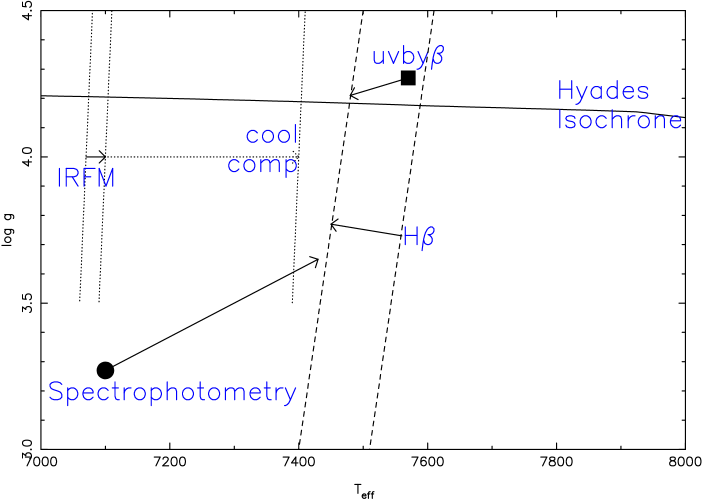
Figure 4: A $T\rm_{eff}$–$\log g$ diagram for 63 Tau. The results from four methods are shown as follows: the filled square is from the Moon & Dworetsky (1985) $uvby\beta$ girds, the filled circle is from spectrophotometric flux fitting, the dashed line that from fitting H$\beta$ profiles and the dotted line the IRFM result. Photometry and Balmer lines agree very well, but are significantly hotter than the results from Spectrophotometry and the IRFM. The solid arrows indicate the effect of using [M/H] = +0.5 models. Now spectrophotometry is in good agreement with photometry and Balmer line, but the IRFM is still significantly lower. However, by introducing a cool companion (5000 K) the IRFM can be brought into agreement with the other methods (dotted arrow). The solid line is the Hyades isochrone, based on the evolutionary calculations of Schaller et al. (1992). (Adapted from Smalley 1996)

4.4 53 Cam

The magnetic Ap star 53 Cam has a rotation period of 8 days and spectroscopic binary orbital period of 6$\frac{1}{2}$ years (Hoffleit & Warren, 1991).

Photometric calibrations give discrepant results: $uvby\beta$ grid of Moon & Dworetsky (1985) gives 10610 $\pm$ 130 K and 4.06 $\pm$ 0.05, while the $uvby$ grid of Smalley & Kupka (1997) gives 8720 $\pm$ 250 K and 4.76 $\pm$ 0.13 for [M/H] = +1.0 and the Kunzli et al. (1997) Geneva calibration gives 8740 $\pm$ 90 K, 4.44 $\pm$ 0.10.

Available flux measurements yield $f\rm_{\oplus}$ = 9.19 $\pm$ 0.73 $\times$ 10^-11 W m^-2. Using the IRFM $T\rm_{eff}$ = 8200 $\pm$ 250 K is obtained for a single star solution. A binary solution would give 8600K for a 6500 K main-sequence secondary, which is in agreement with some of the photometric results.

The analysis by Kochukhov et al. (2004) gave $T\rm_{eff}$ = 8400 $\pm$ 150 K and $\log g$ = 3.70 $\pm$ 0.10, but they found that the results from spectrophotometry and Balmer lines discordant. This demonstrates the important difference between effective temperature as indicated by the emergent fluxes and that obtained from line-forming regions. If the model used is not appropriate to the physical structure of the star’s atmosphere, then the results will disagree.

5 Conclusions

The atmospheric parameters of a star can be obtained by several techniques. By using a combination of these techniques we can assess the quality of our parameter determinations. While some techniques can give precise parameter determinations, the overall accuracy of the values is significantly less and sometimes difficult to evaluate. Realistically, the typical errors on the atmospheric parameters of a star, will be $T\rm_{eff}$ $\pm$100 K (1$\sim$2%) for $T\rm_{eff}$ and $\pm$0.2 dex ($\sim$20%) for $\log g$. For a typical mictroturbulence uncertainty of $\pm$ 0.1km s^-1, these uncertainties give rise to errors of the order of 0.05 $\sim$ 0.1 dex in abundance determinations. Naturally, the exact size of the uncertainty will depend upon the sensitivity of the lines used in the analysis.

It may appear strange, but the effective temperature of a star is not important; it is the T($\tau_{0}$) relationship that determines the spectral characteristics (Gray, 1992). Hence, the parameters obtained from spectroscopic methods alone may not be consistent with the true values as obtained by model-independent methods. This is not necessarily important for abundance analyses of stars, but it is an issue when using the parameters to compare with fundamental values or to infer the physical properties of stars.

References

- Adelman et al. (1989) Adelman S.J., Pyper D.M., Shore S.N., White R.E., Warren W.H., 1989, A&AS, 81, 221
- Adelman et al. (2004) Adelman S.J., Gulliver A.F., Smalley B., Pazder J.S., Younger P.F. et al., 2004, IAUS, 224, 911
- Adelman et al. (2005) Adelman S.J., Gulliver A.F., Smalley B., Pazder J.S., Younger P.F. et al., 2005, these proceedings.
- Alcock et al. (2001) Alcock C., Allsman R.A., Alves D.R., Axelrod T.S., Becker A., et al., 2001, Nature, 414, 617
- Alonso et al. (1994) Alonso A., Arribas S., Martínez-Roger C., 1994, A&A, 282, 684
- Alonso et al. (1996) Alonso A., Arribas S., Martínez-Roger C., 1996, A&A, 313, 873
- Andersen (1991) Andersen J., 1991, A&A Rev., 3, 91
- Blackwell & Lynas-Gray (1994) Blackwell D.E., Lynas-Gray A.E., 1994, A&A, 282, 899
- Blackwell & Shallis (1977) Blackwell D.E., Shallis M.J., 1977, MNRAS, 180, 177
- Blackwell, Petford & Shallis (1980) Blackwell D.E., Petford A.D., Shallis M.J., 1980, A&A, 82, 249
- Blackwell et al. (1990) Blackwell D.E., Petford A.D., Arribas S., Haddock D.J., Selby M.J., 1990, A&A, 232, 396
- Bohlin & Gilliland (2004) Bohlin R.C., Gilliland R.L., 2004, AJ, 127, 3508
- Breger (1976) Breger M., 1976, ApJS, 32, 7
- Burnashev (1985) Burnashev V.I., 1985, Abastumanskaya Astrofiz. Obs. Bull. 59, 83 [III/126]
- Castelli & Kurucz (1994) Castelli F., Kurucz R.L., 1994, A&A, 281, 817
- Ciardi et al. (2001) Ciardi D.R., van Belle G.T., Akeson R.L., Thompson R.R., Lada E.A., Howell S.B., 2001, ApJ, 559, 1147
- Clem et al. (2004) Clem J.L., VandenBerg D.A., Grundahl F., Bell R.A., 2004, AJ, 127, 1227
- Code et al. (1980) Code A.D., Holm A.V., Bottemiller R.L., 1980, ApJS, 43, 501 [II/83]
- Decin et al. (2003) Decin L., Vandenbussche B., Waelkens C., Eriksson K., Gustafsson B., et al., 2003, A&A, 400, 679
- ESA (1997) ESA, 1997, The Hipparcos and Tycho Catalogues, ESA SP-1200
- Fernie (1981) Fernie J.D., 1981, PASP, 93, 333
- Gezari et al. (1999) Gezari D.Y., Pitts P.S., Schmitz M., 1999, Unpublished [II/225]
- Girard et al. (2000) Girard T.M., Wu H., Lee J.T., Dyson S.E., van Altena W.F., et al., 2000, AJ, 119, 2428
- Glushneva et al. (1998) Glushneva I.N., Kharitonov A.V., Knyazeva L.N., Shenavrin V.I., 1992, A&AS, 92, 1
- Gray (1992) Gray D.F., 1992, The observation and analysis of stellar photospheres, CUP.
- Gray (1994) Gray D.F., 1994, PASP, 106, 1248
- Gray & Johanson (1991) Gray D.F., Johanson H.L., 1991, PASP, 103, 439
- Gray & Livingston (1997) Gray D.F., Livingston W.C., 1997, ApJ, 474, 802
- Griffin (1998) Griffin R.F., 1998, Obs, 118, 299
- Griffin & Lynas-Gray (1999) Griffin R.F., Lynas-Gray A.E., 1999, A&A, 282, 899
- Hayes & Latham (1975) Hayes D.S., Latham D.W., 1975, ApJ, 197, 593
- Heiter et al. (2002) Heiter U., Kupka F., van’t Veer-Menneret C., Barban C., Weiss W.W., et al. 2002, A&A, 392, 619
- Hoffleit & Warren (1991) Hoffleit D., Warren Jr W.H, 1991, The Bright Star Catalogue, 5th Revised Ed. [V/50]
- Houdashelt et al. (2000) Houdashelt M.L., Bell R.A., Sweigart A.V., 2000, AJ, 119, 1448
- Jamar et al. (1976) Jamar C., Macau-Hercot D., Monfils A., Thompson G.I., Houziaux L., Wilson R., 1976, Ultraviolet Bright-Star Spectrophotometric Catalogue, ESA SR-27 [III/39A]
- Jiang et al. (2004) Jiang G., DePoy D.L., Gal-Yam A., Gaudi B.S., Gould A., et al., 2004, ApJ, 617, 1307
- Kervella et al. (2004a) Kervella P., Thévenin F., Di Folco E., Ségransan D., 2004a, A&A, 426, 297
- Kervella et al. (2004b) Kervella P., Thévenin F., Morel P., Berthomieu G., Bordé, Provost J., 2004b, A&A, 413, 251
- Kinman & Castelli (2002) Kinman T., Castelli F., 2002, A&A, 391, 1039
- Kochukhov et al. (2004) Kochukhov O., Bagnulo S., Wade G.A., Sangalli L., Piskunov N., et al., 2004, A&A, 414, 613
- Kunzli et al. (1997) Kunzli M., North P., Kurucz R.L., Nicolet B., 1997, A&AS, 122, 51
- Lastennet & Valls-Gabaud (2002) Lastennet E., Valls-Gabaud D., 2002, A&A, 396, 551
- Lester, Gray & Kurucz (1986) Lester J.B., Gray R.O., Kurucz R.L., 1986, ApJS, 61, 509
- Macau-Hercot et al. (1978) Macau-Hercot D., Jamar C., Monfils A., Thompson G.I., Houziaux L., Wilson R., 1978, Supplement to the Ultraviolet Bright-Star Spectrophotometric Catalogue, ESA SR-28 [II/86]
- Magain (1984) Magain P., 1984, A&A, 134, 189
- Mégessier (1994) Mégessier C., 1994, A&A, 289, 202
- Mégessier (1995) Mégessier C., 1995, A&A, 296, 771
- Mendoza (2005) Mendosa B., 2005, AdSpR, 35, 882
- Moon & Dworetsky (1985) Moon T.T., Dworetsky M.M., 1985, MNRAS, 217, 305
- Mozurkewich et al. (2003) Mozurkewich D., Armstrong J.T., Hindsley R.B., Quirrenbach A., Hummel C.A. et al., 2003, AJ, 126, 2502
- Pasinetti-Fracassini et al. (2001) Pasinetti-Fracassini L.E., Pastori L., Covino S., Pozzi A., 2001, A&A, 367, 521 [II/224]
- Patience et al. (1998) Patience J., Ghez A.M., Reid I.N., Weinberger A.J., Matthews, K., 1998, AJ, 115, 1972
- Perevozkina & Svechnikov (1999) Perevozkina E.L., Svechnikov M.A., 1999 [V/118]
- Popper (1980) Popper D.M., 1980, ARA&A, 18, 115
- Ramírez & Meléndez (2005a) Ramírez I., Meléndez J., 2005a, ApJ, 626, 4446
- Ramírez & Meléndez (2005b) Ramírez I., Meléndez J., 2005b, ApJ, 626, 465
- Richichi et al. (2005) Richichi A., Percheron I., Khristoforova M., A&A, 431, 773
- Schaller et al. (1992) Schaller G., Schaerer D., Meynet G., Maeder A., 1992, A&AS, 96, 269
- Sekiguchi & Fukugita (2000) Sekiguchi M., Fukugita M., 2000, AJ, 120, 1072
- Smalley (1993) Smalley B., 1993, MNRAS, 265, 1035
- Smalley (1996) Smalley B., 1996, ASP Conf, 108, 43
- Smalley & Dworetsky (1995) Smalley B., Dworetsky M.M., 1995, A&A, 293, 446
- Smalley & Kupka (1997) Smalley B., Kupka F., 1997, A&A, 328, 349
- Smalley et al. (2002) Smalley B., Gardiner R.B., Kupka F., Bessell M.S., 2002, A&A, 395, 601
- Southworth et al. (2005) Southworth J., Maxted P.F.L., Smalley B., 2005, A&A, 429, 645
- Steffen (1985) Steffen M., 1985, A&AS, 59, 403
- Thompson et al. (1978) Thompson G.I., Nandy K., Jamar C., Monfils A., Houziaux L., Carnochan D.J., Wilson R., 1978, The Science Research Council, U.K. [II/59B]
- VandenBerg & Clem (2003) VandenBerg D.A, Clem J.L., 2003, AJ, 126, 778
- Vasil’yev et al. (1989) Vasil’Yev I.A., Merezhin V.P., Nalimov V.N., Novosyolov V.A., 1989, IBVS, 3308, 1
- Verhoelst et al. (2005) Verhoelst T., Bordé P.J., Perrin G., Decin L., Eriksson K., et al., 2005, A&A, 435, 289
- Zahid et al. (2004) Zahid H.J., Hudson H.S., Fröhlich C., 2004, Solar Physics, 222, 1