Carbon Ignition in Type Ia Supernovae: II. A Three-Dimensional Numerical Model

Abstract

The thermonuclear runaway that culminates in the explosion of a Chandrasekhar mass white dwarf as a Type Ia supernova begins centuries before the star actually explodes. Here, using a 3D anelastic code, we examine numerically the convective flow during the last minute of that runaway, a time that is crucial in determining just where and how often the supernova ignites. We find that the overall convective flow is dipolar, with the higher temperature fluctuations in an outbound flow preferentially on one side of the star. Taken at face value, this suggests an asymmetric ignition that may well persist in the geometry of the final explosion. However, we also find that even a moderate amount of rotation tends to fracture this dipole flow, making ignition over a broader region more likely. Though our calculations lack the resolution to study the flow at astrophysically relevant Rayleigh numbers, we also speculate that the observed dipolar flow will become less organized as the viscosity becomes very small. Motion within the dipole flow shows evidence of turbulence, suggesting that only geometrically large fluctuations ($\sim 1$ km) will persist to ignite the runaway. We also examine the probability density function for the temperature fluctuations, finding evidence for a Gaussian, rather than exponential distribution, which suggests that ignition sparks may be strongly spatially clustered.

1 INTRODUCTION

The leading model for a Type Ia supernova is a carbon-oxygen white dwarf that accretes matter from a binary companion at a sufficiently high rate that it is able to grow to the Chandrasekhar mass and explode (eg., Hillebrandt & Niemeyer, 2000). Much of the research in recent years has focused upon the computationally challenging problem of how a nuclear fusion flame, once formed in the white dwarf interior, succeeds in burning a sufficient fraction of its mass to ⁵⁶Ni and intermediate mass elements to power a healthy explosion and give a credible light curve and spectrum (eg., Gamezo et al., 2003; Plewa et al., 2004; Röpke & Hillebrandt, 2005). Equally important, however, is just how the flame ignites. A flame starting from a single point at the middle, a single point off center, and a multitude of points isotropically distributed around the center will all give qualitatively different results (Niemeyer & Hillebrandt, 1995; Niemeyer, Hillebrandt, & Woosley, 1996; Plewa et al., 2004; García-Senz & Bravo, 2005; Röpke et al., 2005). The first numerical simulation of carbon ignition suggested central ignition (Höflich & Stein, 2001), but may not have correctly represented the pre-explosive convective flow because of its restricted geometry. Analytic calculations have supported the idea of off-center ignition, probably at multiple points (Garcia-Senz & Woosley, 1995; Woosley, Wunsch, & Kuhlen, 2003; Wunsch & Woosley, 2004), but require their own assumptions, for example the persistence of fluctuations and the existence (or non existence) of an ordered background flow.

The numerical simulation of carbon ignition in this environment involves a different sort of physics, and optimally, a different sort of computer code than the flame propagation problem. The fluid motion is very subsonic (Mach number less than about 0.01) and the density contrasts that must be followed are small $\sim 10^{-5}$. Both can pose problems for compressible hydrodynamics codes. The simulation must be followed in 3D for a long time and this is challenging for a code that is Courant limited by the speed of sound. However, these same circumstances are very favorable for anelastic hydrodynamics, which is Courant limited by the fluid velocity. In § 3.1 we describe the implementation for the supernova problem of a 3D anelastic code that has previously been employed to study the sun (Glatzmaier, 1984), the earth’s geodynamo (Glatzmaier & Roberts, 1995), and planetary convection (Sun, Schubert, & Glatzmaier, 1993). This code is based on spectral methods that greatly improve the effective resolution over ordinary spatial grids. As we shall see, resolution is a big issue since the Reynolds number in the star is Re $\sim 10^{14}$ (Woosley, Wunsch, & Kuhlen, 2003), far beyond what can be achieved in any presently existing code. We are thus only able to glimpse large scale features (§ 4.2) and hints of complex structures beneath.

Nevertheless, we come to some interesting conclusions. The overall convective flow, for the range of Reynolds numbers that is accessible, is dipolar. This has been seen before in different environments (eg., Woodward et al., 2003), but the present study is the first to find it in numerical simulations of Type Ia supernova ignition. This flow suggests the supernova may ignite in a lop-sided fashion, but there are many caveats (§ 5). We are also able to determine the probability density function (PDF) of the temperature fluctuations and show that it is Gaussian. This has important implications for the number of ignition points (Woosley, Wunsch, & Kuhlen, 2003). We also call attention to the turbulence that exists in the outgoing “jet” of the dipole (§ 4.4). Superimposed on the flow which carries the sparks that will ignite the supernova is the beginning of what looks to be a Kolmogorov cascade to smaller scales. This will limit the size of the temperature fluctuation that is necessary to ignite the star off center. Sparks that are too small will be dissipated by turbulence before they run away. It will take a finer resolved study than the present one to conclusively address the issue, but it may be that the smallest ignition points are of resolvable size, $\sim 1$ km.

2 The Initial Model

In our implementation of the anelastic approximation we solve for thermodynamic perturbations to an isentropic, constant reference state (see Section 3.2). The one-dimensional background state has been determined here using an implicit hydrodynamics code, kepler(Weaver, Zimmerman, & Woosley, 1978). A white dwarf composed of 50% carbon and 50% oxygen was allowed to accrete (carbon and oxygen) at a rate of 10^-7 ${\mathrm{M}_{\odot}}\ \,{\mathrm{yr}}\ ^{-1}$ . When the central density and temperature reached $3.2\times 10^{9}$ g cm^-3 and $2.5\times 10^{8}$ K, nuclear energy generation from carbon fusion exceeded the plasma neutrino loss rate. The excess energy was carried away by convection. At this point the star’s mass was 1.38 $\mathrm{M}_{\odot}$ and its radius 1580 km.

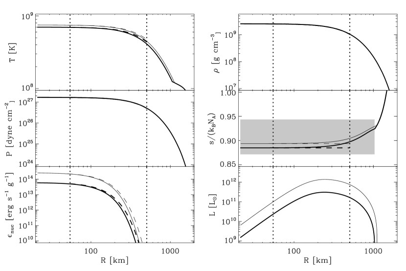
Figure 1: The one-dimensional kepler model: Temperature, density, pressure, entropy per baryon, nuclear energy generation, and radiative luminosity as a function of radius. Thick lines are for the $T_{c,8}=7$, thin lines for the $T_{c,8}=7.5$ snapshot. The vertical dotted lines denote the inner and outer boundary of the three-dimensional anelastic simulation. Dashed lines indicate the isentropic reference state (see Section 3.2). The gray region in the entropy plot demarcates the range of radii that are convectively unstable in the kepler model.

Over the next 5000 years the central temperature rose and the extent of the convective core grew, from initially less than 1%, to 0.45 $\mathrm{M}_{\odot}$ when the central temperature was $4\times 10^{8}$ K (2 years before explosion), and to 0.95 $\mathrm{M}_{\odot}$ when the central temperature was $6\times 10^{8}$ K (3 hours before explosion). During this ramp up to runaway, neutrino losses and radiation transport to the surface of the star were negligible and a small amount of energy went into expansion (the central density first increased slightly then declined by 15%). Most of the energy went simply into raising the temperature of the convective core and extending its extent (Baraffe et al., 2004).

When the central temperature reached $7.5\times 10^{8}$ K, the convective core was 1.15 $\mathrm{M}_{\odot}$ (1040 km) and the central density, $2.7\times 10^{9}$ g cm^-3. The net binding energy of the white dwarf (internal plus gravitational) was $4.36\times 10^{50}$ erg and the pressure scale height was 450 km. If mixing length convection was left on, the explosion occurred 190 s later. Radial profiles of $T$, $\rho$, $P$, $sm_{p}/k_{B}$ (entropy per baryon), $\epsilon_{\rm nuc}$, and $L$ are shown in Figure 1, at two different times: when the central temperature has reached $T_{\rm c,8}=7$ and $T_{\rm c,8}=7.5$. It is interesting to note that though the entropy in the convective region in the Kepler model was constant to within 1%, the convective flux was not constant for any appreciable span of radii. Two-thirds of the total nuclear energy ($3.0\times 10^{45}$ erg s^-1) was produced within the inner 0.01 $\mathrm{M}_{\odot}$ , but the luminosity itself rose to a maximum of $2.6\times 10^{45}$ erg s^-1 and declined to approximately zero at the outer edge of the convective core. Almost all of the nuclear energy is lost in transit to heating along the way.

3 A THREE DIMENSIONAL MODEL USING ANELASTIC HYDRODYNAMICS

3.1 The Code and its Modifications

The code used for the simulations presented here is based upon the anelastic hydrodynamics code of Glatzmaier (1984). The hydrodynamic equations are implemented in a fully spectral manner, expanding all quantities in spherical harmonics to cover the angular variations, and in Chebyshev polynomials for the radial dependence. Although a spectral method in spherical coordinates is more difficult to implement than one based on a finite differencing scheme on a Cartesian grid, and also requires more communication on a multi-processor parallel computation system, a major advantage is the greater efficiency provided by the spectral method. To achieve a modest accuracy of a few percent, spectral methods typically require only half as many degrees of freedom per dimension as a fourth order finite difference method (Boyd, 2000). Chebyshev polynomials are defined on a domain from $-1$ to $+1$, which in this code is mapped to the inner and outer boundary of the convective region. Unfortunately, the current implementation of spherical coordinates prohibits the computational domain from extending all the way to the origin, since $1/r$ terms in the angular derivatives lead to divergences. A central sphere is cut out and replaced by an inner impermeable boundary condition, even in situations where the convective region includes the center of the star (see 3.3). The code employs a rhomboidal truncation of the spherical harmonic modes, which means that every longitudinal Fourier mode ($e^{im\phi}$) has the same number of latitudinal associated Legendre functions ($P_{l}^{m}(\cos\theta)$). A rhomboidal truncation scheme is easier to parallelize than a more conventional triangular truncation ($-l\leq m\leq+l$), and it ensures that the latitudinal resolution is the same for all longitudinal modes.

In this formulation of anelastic hydrodynamics, the mass, momentum, and entropy conservation equations are expanded in a power series around a one-dimensional, constant, and isentropic reference state, and only the lowest orders terms are retained. The reference state is determined by the one-dimensional stellar evolution code kepler (see Sections 2 and 3.2). In the following all reference state quantities are barred, and all perturbations denoted with a $\delta$. The fundamental quantities in this code are the entropy ($\delta s$) and pressure ($\delta P$) perturbations. In order to relate these to the more familiar quantities density and temperature, we require an equation of state.

$$\delta T = \left(\overline{\frac{\partial T}{\partial s}}\right)_{P}\delta s+\left(\overline{\frac{\partial T}{\partial P}}\right)_{s}\delta P$$ (1a)

$$\delta\rho = \left(\overline{\frac{\partial\rho}{\partial s}}\right)_{P}\delta s+\left(\overline{\frac{\partial\rho}{\partial P}}\right)_{s}\delta P$$ (1b)

The equation of state is specified by four thermodynamic partial derivatives, which are part of the time-independent reference state and depend only on radius. We use the Helmholtz equation of state code Timmes & Swesty (2000) to calculate these derivatives for a given kepler reference state.

In total, we solve for two thermodynamic variables ($\delta s$ and $\delta P$), the perturbation of the gravitational potential ($\delta\Phi_{g}$), and the three components of the fluid flow velocity ($v_{r},v_{\theta},$ and $v_{\phi}$). The relevant equations are:

$$\mathbf{\nabla}\cdot(\bar{\rho}\mathbf{v}) = 0$$ (2a)

$$\bar{\rho}\frac{\partial\mathbf{v}}{\partial t} = -\mathbf{\nabla}\cdot(\bar{\rho}\mathbf{v}\otimes\mathbf{v})-\bar{\rho}\mathbf{\nabla}(\frac{\delta P}{\bar{\rho}}+\delta\Phi_{g})$$ (2b)

$$-\left(\frac{\partial\bar{\rho}}{\partial s}\right)_{P}\delta s\;\bar{g}\;\mathbf{\hat{r}}+2\;\bar{\rho}\;\mathbf{v}\times\mathbf{\bar{\Omega}}$$

$$+\mathbf{\nabla}\cdot\left(2\bar{\rho}\bar{\nu}(\bar{\mathbf{\mathsf{E}}}-\frac{1}{3}(\mathbf{\nabla}\cdot\mathbf{v})\mathbf{\mathsf{I}})\right)$$

$$\bar{\rho}\bar{T}\frac{\partial\delta s}{\partial t} = \mathbf{\nabla}\cdot(\bar{\kappa}\bar{\rho}\bar{T}\mathbf{\nabla}\delta s)-\bar{T}\mathbf{\nabla}\cdot(\bar{\rho}\delta s\mathbf{v})$$ (2c)

$$+\bar{\rho}(\bar{\epsilon}_{\rm nuc}+\delta\epsilon_{\rm nuc})$$

$$-\bar{\rho}(\bar{\epsilon}_{\nu}+\delta\epsilon_{\nu})$$

$$\mathbf{\nabla}^{2}\delta\Phi_{g} = 4\pi G\delta\rho$$ (2d)

Here $\bar{\mathbf{\mathsf{E}}}$ is the rate of strain tensor, $\mathbf{\mathsf{I}}$ the identity matrix, and $\bar{\Omega}$ the reference state rotation vector. In order to allow for the differential heating of hot and cold convective elements, we have included a first order perturbation term in addition to the one-dimensional background nuclear burning rate. This background energy generation rate is determined from the kepler output and fitted to a power law, $\rho T^{\alpha}$. For the simulations discussed in this paper $\alpha$ is approximately equal to 27. The total energy generation rate is then:

$$\epsilon_{\rm nuc}=\bar{\epsilon}_{\rm nuc}+\epsilon^{\prime}_{\rm nuc}\propto\bar{\rho}\bar{T}^{\alpha}\left(1+\frac{\delta\rho}{\bar{\rho}}+\alpha\frac{\delta T}{\bar{T}}\right)$$ (3)

Energy losses to neutrinos ($\bar{\epsilon}_{\nu},\epsilon_{\nu}$) act as a sink in the entropy conservation equation. Results from one dimensional simulations indicate that these neutrino losses are negligible (Section 2), and we have included them in Equation (2) only for completeness.

Momentum and energy transport at scales below our spatial resolution are handled by introducing artificially high viscous and thermal diffusion coefficients $\bar{\nu}$ and $\bar{\kappa}$. In our simulation the Prandtl number (Pr $=\bar{\nu}/\bar{\kappa}$) is kept at unity, and $\bar{\nu}$ and $\bar{\kappa}$ are lowered as much as possible for a given resolution (see Section 3.3). These turbulent diffusion coefficients also enter in the calculations of the dimensionless numbers characterizing the fluid flow, the Rayleigh (Ra) and Reynolds (Re) numbers.

$${\rm Ra} \sim \frac{D^{3}g\Delta s}{c_{P}\bar{\nu}\bar{\kappa}}$$ (4a)

$${\rm Re} \sim \frac{vD}{\bar{\nu}}$$ (4b)

Here $D$ is the depth of the modeled region and $\Delta s$ the change in specific entropy across $D$. Ra is proportional to the ratio of buoyancy to diffusion forces, and Re is proportional to the ratio of inertial to viscous forces. A large Rayleigh number indicates very vigorous convection, and a large Reynolds number indicates a highly turbulent flow. Typical Rayleigh numbers in the central convective region of a pre-SNIa white dwarf are around $10^{25}$ and typical Reynolds numbers around $10^{14}$ Woosley, Wunsch, & Kuhlen (2003). Use of the turbulent viscous and thermal diffusion coefficients instead of the true molecular ones greatly reduces the magnitude of Ra and Re that are achievable with this code. Our simulations reach Ra $\approx 10^{7}$ and Re $\approx 1500$, just entering the turbulent convective regime, but a far cry from the true physical conditions (see Section 4).

3.2 Mapping the Background State into the 3D-Code

From a given kepler output (Section 2) we extract the density and pressure profiles for the region of interest. For numerical stability, we then fit a polytrope ($P(r)=K\rho(r)^{1+1/n}$) to this profile, and solve the resulting Lane-Emden equation for $\bar{P}(r)$ and $\bar{\rho}(r)$. Using the Helmholtz equation of state code Timmes & Swesty (2000) we solve for the corresponding temperature profile $\bar{T}(r)$ and for the thermodynamic partial derivatives (see Section 3.1). Since the kepler models are close to, but not completely isentropic we also determine a volume averaged background state entropy. This quantity is useful for comparisons with analytical models, but never used in the 3D anelastic calculation itself.

3.3 Models and Procedures

Analytical considerations show Woosley, Wunsch, & Kuhlen (2003) that the ignition of the final deflagration leading to the supernova explosion is likely to start somewhere off-center at about $150-200$ km. We have chosen to model a region extending from $50$ km to $500$ km. The boundary conditions at these radii are impermeable and stress-free ($v_{\perp}=0$ and $\frac{\partial}{\partial r}\left(\frac{v_{\parallel}}{r}\right)=0$).

Since almost all of the energy generation and the most vigorous convection occur at radii less than $200{\mathrm{km}}\$, we don’t expect this outer boundary at $500{\mathrm{km}}\$ to unduly influence our results. The central boundary is more problematic, since in a real star nothing prevents fluid from streaming through the center. In our model cold sinking fluid will splash around the inner boundary. Only by extrapolating from conditions outside $R=50{\mathrm{km}}\$, can we say anything about the flow pattern right at the center.

Table 1: Summary of models

Name	$T_{c,8}$	$n_{\rm max}$	$m_{\rm max}$	$l_{\rm max}$	$\Delta t$	$\Omega$	Description
					[s]	[rad s-1]
C7	7.0	241	42	85	70.36	0.0	fiducial model
C7rot	7.0	…	…	…	77.06	0.167	rotating background state
C75	7.5	…	…	…	40.90	0.0	higher central temperature

Additional boundary conditions are necessary for the entropy equation. Since the radial velocity, and with it, the convective heat flux, is forced to zero at the inner and outer boundary, turbulent diffusion is the only mechanism by which energy can be transported across these boundaries. This heat diffusion is carried by a negative radial entropy gradient. At the inner boundary the kepler luminosity is essentially zero, and so we set $d\delta s/dr=0$ there. At the outer boundary the kepler luminosity is non-zero ($\sim 10^{45}$ - $10^{46}$ erg/s), but still much less than the total integrated energy generation rate in the simulated volume. The excess energy deposited on the grid gradually leads to an increase in central temperature as described in Section 2. Our anelastic model, however, is constructed around a time-independent reference state. The inability to follow the evolution of the background state forces us to examine several “snapshots” in the evolution. In this paper we consider two different central temperatures: $T_{c,8}=$ 7.0 and 7.5. Our goal is to establish a pseudo-steady-state at each of these epochs, which, while being physically unrealistic, might still allow us to infer something about the spectrum of temperature fluctuations and the global flow pattern. To do this we compensate for the excess energy by adjusting the outer luminosity to balance the total energy generation rate in our computational domain. In order to establish a sufficiently large negative entropy gradient, $\delta s$ is forced to become negative at the outer boundary. This is artificial – in a real white dwarf the entropy gradient would remain adiabatic throughout the convection zone. The compromise was necessary in order to achieve a model in near steady state that would run stably for a long time.

Figure 2: The horizontally and time averaged radial, angular, and total velocities as a function of radius in the C7 simulation. The solid line shows the root mean square, the dashed lines the minimum and maximum, and the dotted line (only in the total velocity plot) the mean velocities in each radial shell. The radial velocity is forced to zero at the inner boundary (see text for discussion).

Figure 3: Horizontally averaged mass-weighted radial profiles of $\delta X/\bar{X}$ (solid, left ordinate) and $\delta X$ (dotted, right ordinate), where $\delta X$ is the entropy, pressure, density, and temperature perturbation (clockwise from top left).

In order to allow the model to find a stable solution quickly, we begin with large turbulent diffusivities and gradually turn them down, in small enough increments that the code is able to find a new stable solution. This decrease raises our operational Rayleigh and Reynolds numbers. To ensure numerical stability the diffusivities must remain large enough to prevent a build-up of entropy at the smallest scales. We continue to lower the diffusivities to the smallest value that can be accommodated with a given spatial resolution. We then continue to evolve the model at fixed diffusivity. In this manner we found pseudo-steady-states for both temperature snapshots. The results presented here are from only the last $84,000$ time steps, whereas the relaxation phase of the simulation took about $175,000$ time steps. The long duration of the relaxation ensures that any “memory” of the initial conditions of the simulation is completely erased.

We considered three models: C7, a non-rotating model with a central temperature of $T_{\rm c,8}$=7.0, C7rot, identical to C7, except that the background state is rotated rigidly with an angular velocity $\Omega=0.167$ rad/s (Ekman number $\sim 7\times 10^{-4}$, see Section 4.5), and C75, non-rotating, but with $T_{\rm c,8}$=7.5. The resolution was the same in all three models: $n_{\rm max}=237$ Chebyshev polynomials in the radial direction, and spherical harmonics up to $m_{\rm max}=42$ and $l_{\rm max}=85$. As we show below (Section 4), typical plume velocities are $\sim 50$ km/s and $\sim 100$ km/s in the C7 and C75 simulations, respectively, which translates to convective turnover times of $t_{\rm to}=2(R_{\rm outer}-R_{\rm inner})/v_{\rm plume}=$ 18 and 9 seconds respectively. The two simulations are evolved for about 70 and 40 seconds star time, so for roughly four convective turnovers in both cases. The parameters of each simulation are summarized in Table 1.

4 RESULTS

4.1 Velocities and Thermodynamic Perturbations

In order for the anelastic approximation to be valid, the fluid flow must remain subsonic and variations from the reference state must be small, $<\sim 1\%$. The time and angle averaged (over the last 84000 time steps) total, radial, and angular velocities are plotted as a function of radius in Figure 2. The horizontal mean as a function of radius of the absolute value of total velocity increases from a minimum of about 50 km/s at $R=400$ km up to about 90 km/s near the center. The maximum velocity achieved anywhere on the grid is 150 km/s. This is much less than the sound speed of $c_{\rm sound}\sim$8000 km/s, so the condition of subsonic flow is satisfied.

Figure 3 shows horizontally averaged mass-weighted radial profiles of the thermodynamic perturbations at the end of the C7 simulation. The top two plots show the two independent variables, the entropy and pressure perturbations. The two perturbations are comparable in magnitude, and both lie below the 1% level. The maximum entropy and pressure perturbations in the whole volume, of course, are higher: $(|\delta s|/\bar{s})_{\rm max}=0.015$ and $(|\delta P|/\bar{P})_{\rm max}=0.003$. The largest entropy perturbation is negative, occurs at the outer boundary, and is caused by the large negative entropy gradient required to balance the total energy generation, as explained in Section 3.3. Using Eq. (1) we can determine temperature and density fluctuations from the entropy and pressure perturbations. These are shown in the lower two plots of Figure 3. Since $\left(\overline{\frac{\partial\ln T}{\partial\ln s}}\right)_{P}\gg\left(\overline{\frac{\partial\ln T}{\partial\ln P}}\right)_{s}$ and $\left(\overline{\frac{\partial\ln\rho}{\partial\ln s}}\right)_{P}\ll\left(\overline{\frac{\partial\ln\rho}{\partial\ln P}}\right)_{s}$,

$$\delta T/\bar{T}\approx\left(\overline{\frac{\partial\ln T}{\partial\ln s}}\right)_{P}\delta s/\bar{s},$$ (5a)

$$\delta\rho/\bar{\rho}\approx\left(\overline{\frac{\partial\ln\rho}{\partial\ln P}}\right)_{s}\delta P/\bar{P}.$$ (5b)

Figure 4: Variance of entropy perturbation versus spherical harmonic wavenumber $l$ at the end of the C7 simulation. The dotted line is a $l^{-5/3}$ power law, as expected for a Kolmogorov turbulent spectrum.

For the conditions inside the simulated region, $\left(\overline{\frac{\partial\ln T}{\partial\ln s}}\right)\approx 3.5$ and $\left(\overline{\frac{\partial\ln\rho}{\partial\ln P}}\right)_{s}\approx 0.75$. The largest positive temperature and density perturbation is 1.5% and 0.7%, respectively. Since all thermodynamic perturbations remain below the few percent level, we conclude that the anelastic approximation is indeed a valid one for the problem at hand.

Our resolution of $n_{\rm max}=237$, $m_{\rm max}=42$, and $l_{\rm max}=85$ allowed us to lower the diffusivities to $\bar{\kappa}=\bar{\nu}=5\times 10^{11}{\rm cm}^{2}/s$, corresponding to Rayleigh and Reynolds numbers of Ra $=\sim 10^{7}$ and Re $=\sim 1500$, in all three simulations. The transition from laminar to turbulent flow generally occurs close to Re=2000, so our simulations have not quite reached the regime of fully turbulent convection, but aren’t fully laminar either. In fact, we see about $2/3$ of an order of magnitude of a Kolmogorov turbulent cascade in an angular power spectrum of entropy perturbation, Figure 4. The turbulent cascade begins at $l=10$ and extends down to $l=50$.

While the requirements of a time-independent background state and small perturbations prevent us from following the increase of the central temperature all the way to the point where localized flames develop, we can look at the C75 snapshot to get an idea of what the fluid flow looks like at a higher central temperature of $7.5\times 10^{8}$ K. This study employed the same resolution as in the C7 simulation, but with the more energetic background state, we were only able to lower the diffusivities to $\bar{\kappa}=\bar{\nu}=8.5\times 10^{11}{\rm cm}^{2}/s$. Due to the strong temperature dependence of the nuclear energy generation rate, the convection is much more vigorous in the C75 simulation. Both the velocities and thermodynamic perturbations are larger than in the C7 simulation. The mean velocity now ranges from 70 to 130 km/s, and the maximum velocity on the grid is 276 km/s. These numbers and their temperature scaling agree well with the analytic expectations (Woosley, Wunsch, & Kuhlen, 2003). Typical thermodynamic perturbations have also increased: the shell averaged temperature fluctuation reaches 2% at the innermost radial bin, with the largest positive perturbation reaching 4.4%. Higher temperature perturbations and larger radial velocities increase the likelihood of an off-center supernova ignition. This possibility is further discussed in Section 4.4.

4.2 Flow Patterns

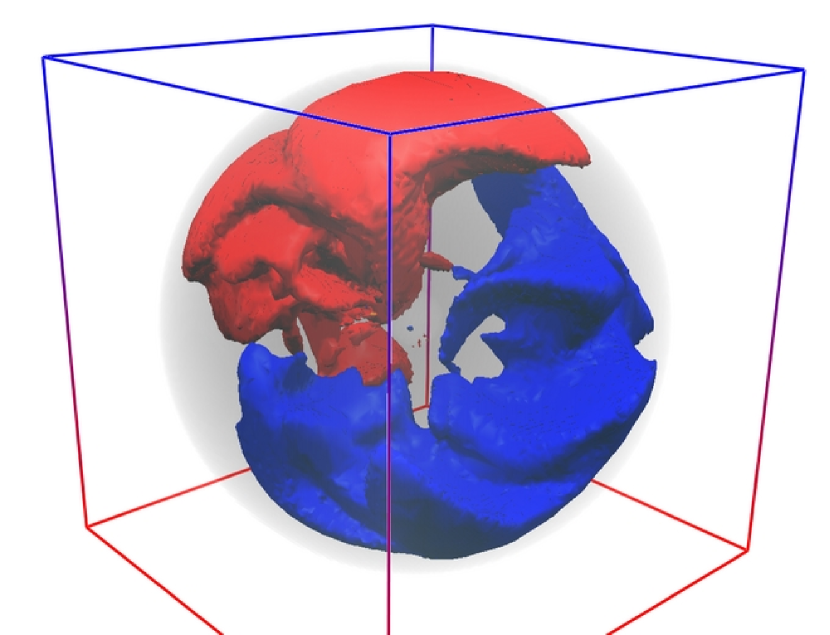
Figure 5: Two iso-velocity surfaces at $|v_{r}|=40$ km/s. The sharp division between infalling (red) and outflowing (blue) material clearly demonstrates the dipole nature of the flow.

The most striking feature of our calculation is a large coherent dipolar circulation. Figure 5 shows a three-dimensional representation of this flow - two iso-radial-velocity surfaces at $v_{r}=\pm 40$ km/s. The outflowing surface (blue) is predominantly located in one hemisphere, the inflowing surface (red), in the other. The dipole nature of the flow can also be seen in Figure 6, which shows two-dimensional equatorial and meridional slices of the temperature fluctuation and the radial component of velocity.

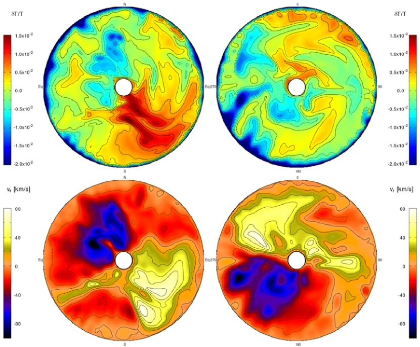
Figure 6: Slices of $\delta T$ (top) and $v_{r}$ (bottom), in meridional (left) and equatorial (right) planes in the non-rotating $T_{\rm c,8}=7$ simulation. Solid contours denote positive, dashed ones negative values.

In the non-rotating models there is no preferred axis in the calculation. The expansion in spherical harmonics might be expected to produce an artificial preferred axis along $\theta=0$, but the observed dipole is not aligned with this axis. Neither is it aligned with any perturbation in the initial conditions. The only explanation is some form of “spontaneous symmetry-breaking”, growing from numerical noise in the calculation.

Admittedly, we cannot address precisely the nature of the flow at the center with our method. As explained in Section 3.3, we solve the anelastic hydrodynamics equations subject to a solid inner boundary condition, which we have placed at $R=50$ km. The sharp drop in the radial velocity component at $R<100$ km/s is artificial, caused by the solid inner boundary condition. The actual radial velocity component at the center can be obtained by extrapolation of its value at 100 km to the origin, as suggested by the large r.m.s. angular velocities near the center. This implies that the center of the star is not at a calm region at all, as one might expect from one-dimensional calculations or multidimensional calculations that do not carry a full 360 degrees. Similar conclusion were reached by a recent 2D anelastic study of convection in the interior of giant gas planets (Evonuk & Glatzmaier, 2005).

4.3 The Temperature Fluctuation Spectrum

Figure 7: The probability distribution of temperature fluctuation evaluated in three constant radius shells (485, 279, and 75 km), when the central temperature is $T_{c,8}$ = 7.0. The y-axis shows the fraction of the area in this shell that intersects fluid elements with temperatures deviating by the amount shown from the mean, divided by the root-mean-square of the temperature fluctuations in that shell. The thin solid and dashed lines show best-fit Gaussian and Exponential PDF, respectively. Only positive fluctuations were used in the fit, and the PDF were constrained to be centered at zero.

As discussed in Woosley, Wunsch, & Kuhlen (2003), the nature of the probability density function (PDF) of temperature fluctuations is important for determining whether the supernova explosion will have one or multiple ignition points. The sharper the high temperature tail of the PDF, the more material there is with temperature just a bit less than the ignition temperature of the first flame.

We have numerically estimated the temperature fluctuation PDF in our simulation for constant radius shells of thickness $\delta R\simeq 2$ km. In each shell we subtract from every temperature fluctuation the mean $\langle\delta T\rangle$, divide by the r.m.s. $\delta T_{\rm rms}$, and use the resulting quantity as our independent variable: $(\delta T-\langle\delta T\rangle)/\delta T_{\rm rms}$. We then determine the PDF by calculating the fraction of volume of the shell occupied by a given fluctuation and dividing by the total volume of the shell. The resulting PDF at three radii (485, 279, and 75 km), corresponding to 20 km from the top, the center of the modeled region, and 20 km from the bottom, are shown as histograms in Figure 7. We have found best-fitting Gaussian distribution (GPDF) and exponential distribution (EPDF) and plotted them as thin solid and dashed lines, respectively. The PDF were fit via simple $\chi^{2}$ minimization, constrained to be centered at $\delta T=\langle\delta T\rangle$, and only the positive fluctuations were used in the fit.

In all three locations the GPDF produced a better fit than the EPDF. None of the fits match the distribution perfectly over the entire range of positive fluctuations, but in particular in the $R=75$km shell the Gaussian fit follows the distribution out to $3.5\delta T_{\rm rms}$. The measured distributions at $R=485$ and 279 km exhibit a strong excess of negative temperature fluctuations over either GPDF or EPDF. This excess is entirely composed of downwards flowing material, making up the return current of the global dipole flow described in Section 4.2.

Niemela et al. (2000) experimentally determined the temperature fluctuation PDF in an incompressible fluid (cryogenic helium at 4 K) as a function of Rayleigh number. At Rayleigh numbers comparable to the ones we have simulated in this study, they also found a Gaussian PDF. At higher Rayleigh number, however, they observed a transition to an Exponential PDF, which remained intact all the way up to Ra $\sim 10^{15}$, the limit of their experiment. Even this is many orders of magnitude below the Ra $\sim 10^{25}$ expected in the centers of white dwarfs, and for all practical purposes the true nature of the temperature fluctuation PDF before the onset of explosive carbon burning must be considered unknown. Further numerical studies at higher Rayleigh numbers are necessary, and may well detect a transition to an exponential PDF.

4.4 The Size and Persistence of Temperature Fluctuations

While the PDF captures how rare a temperature fluctuation is, averaged over space and time, it contains no information about the size and duration of these fluctuations. The persistence of a fluctuation being carried outward is of crucial importance in determining how far from the center the hot spot will run away and ignite the supernova explosion. A hot spot of a given size will be shredded to pieces on a timescale set by the degree of turbulence within the outflow. Together with the laminar outflow velocity, this time scale sets the maximum distance from the center that a hot spot can reach. As we discussed in Section 4.1, we see in our simulations the beginning of a turbulent cascade. Unfortunately, our resolution is nowhere near adequate to follow this cascade from the integral length scale (the size of the largest eddies) all the way down to the Kolmogorov scale (the smallest eddies). We can, however, make use of scaling relations to infer the minimum size fluctuations that will survive out to a given distance from the center.

As discussed by Woosley, Wunsch, & Kuhlen (2003), the spots within the dipole flow that runaway first will be those in which heating by burning just compensates cooling by adiabatic expansion. This consideration, plus a dipole flow speed of approximately 50 - 100 km s^-1, naturally gives ignition about 100 km out from the center of the star.

Within the dipole flow we find a residual random velocity field. The smallest resolved eddies have a length scale of about 50 km and a typical velocity of about 10 km s^-1. Assuming Kolmogorov-Obukhov scaling ($v\propto L^{1/3}$) we can extrapolate to below our resolution limit. We estimate that an eddy 1 km in size will turn over in about 1 second. Smaller eddies will turn over faster, so we take this as a characteristic volume for the fluid that will mix during the 1 to 2 seconds it takes a hot perturbation to move to the ignition radius – 100 km.

All these numbers will require a much better resolved calculation to be taken precisely, but they suggest that the perturbations that ignite the runaway will be moderately large, $\sim 1$ km, a value that might even be resolved in future numerical studies.

Our results also show significant correlation between hot spots. They are not scattered randomly throughout the dipole flow, but concentrated near its axis. Temperature differences will be amplified in the subsequent runaway by the high power of the reaction rate temperature sensitivity, but a reasonable picture of the ignition might be a single, broad, off-center “plume” rather that multiple hot spots.

4.5 The Effect Of Rotation

In addition to the non-rotating models discussed in the previous sections, we also calculated one model (C7rot) with a rigidly rotating background state. Rotation is introduced into the simulation by solving the anelastic conservation equations in a rotating reference frame. This results in the Coriolis force term on the right hand side of Eq.(2b) of $2\bar{\rho}\;\mathbf{v}\times\mathbf{\bar{\Omega}}$, where $\mathbf{\bar{\Omega}}$ is the reference state rotation rate vector in rad/sec. The centrifugal term ($\bar{\rho}\;\mathbf{\bar{\Omega}}\times\mathbf{\bar{\Omega}}\times\mathbf{r}$) is neglected, because it is usually much smaller than the gravitational force.

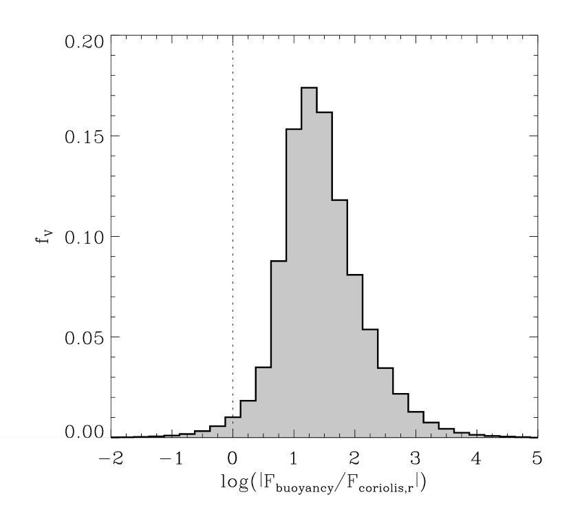
Figure 8: Distribution (volume fraction) of the ratio of the buoyancy force ($-\mathbf{g}\;\delta\rho/\bar{\rho}$) to the radial component of the Coriolis force ($2\;(\mathbf{v}\times\mathbf{\bar{\Omega}})_{r}$). Material to the left of the dotted vertical line experiences a Coriolis force that is stronger than the local buoyancy force.

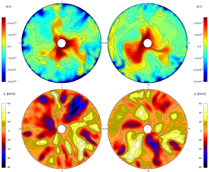
Figure 9: Like Figure 6, but for the C7rot simulation. A rotating background state seems to break up the dipole flow.

Accreting white dwarfs are thought to rotate quite rapidly, with rotation rates approaching Keplerian at the surface (eg. Yoon & Langer, 2004). In the kepler model which is the basis for this anelastic study, the Keplerian rotation rate at the surface is $\Omega_{0}=(GM/R^{3})^{1/2}=5.6$ rad/sec. We are interested in determining what effect even a small amount of rotation has on the dipole flow that we observed in the non-rotating simulations. For this purpose, we chose a moderate background rotation rate of 0.167 rad/sec, only 3% of $\Omega_{0}$. As we shall see, even this comparatively small amount of rotation has an appreciable effect upon the fluid flow. At the outer boundary of our simulation the ratio of centrifugal to gravitational force is $\bar{\Omega}^{2}R^{3}/(GM)=7\times 10^{-5}$, justifying the omission of the centrifugal force term. The importance of the coriolis force relative to buoyancy forces is addressed in Figure 8. We have plotted the fraction of the total simulated volume at a given ratio of buoyancy force ($-\bar{\mathbf{g}}\delta\rho/\bar{\rho}$) to the radial component of coriolis force versus the logarithm of this ratio. This plot shows that buoyancy dominates coriolis forces for most of the simulated volume: only for 1.3% of the total volume does the radial component of the coriolis force exceed the buoyancy force. Two further dimensionless numbers characterize the importance of rotation. The Ekman number is a measure of the relative importance of viscous to Coriolis, and the Rossby number of inertial to rotational forces.

$${\rm Ek}\sim\frac{\bar{\nu}}{2\mathbf{\bar{\Omega}}D^{2}}$$ (6a)

$${\rm Ro}\sim\frac{v}{2D\Omega\sin{\theta}},$$ (6b)

where $\theta$ is the co-latitude. We have Ek $\approx 7\times 10^{-4}$, and at the equator Ro=1 or 1/3, depending on whether we use $v_{\rm max}$ or $v_{\rm mean}$.

Even though the centrifugal and coriolis forces are small compared with gravity and buoyancy, respectively, the rotating background state significantly alters the flow in the simulation. Figure 9 shows equatorial and meridional slices of temperature perturbation and radial velocity for the C7rot simulation. A comparison with Figure 6 shows that the dipole flow has pretty much disappeared. Instead of a well defined outflow (inflow) in the lower right (upper left) quadrant of the meridional slice in the C7 simulation, both inflowing and outflowing plumes can be found in all four quadrants of the same slice in the C7rot simulation. The temperature fluctuations in C7rot are also broken up into multiple hot and cold spots, instead of one hot and one cold plume in C7. Two-dimensional simulations at a much higher Rayleigh number show a transition from a dipole to a differentially rotating longitudinal flow as the rotation rate is increased (Evonuk & Glatzmaier, 2005). It is important to note, however, that flow through the center might still be possible in a different configuration. The temperature fluctuations and convective velocities are of the same order as in the C7 simulation, and the results of Section 4.3 and 4.4 will continue to hold as long as there is at least one central outflow of hot material. An asymmetric supernova explosion, however, becomes less likely in the absence of a strong dipole flow.

5 CONCLUSIONS

Three-dimensional studies at moderate Rayleigh number ($\sim 10^{7}$) of carbon ignition in the highly degenerate core of a white dwarf star show a dipole nature to the flow. If such a flow pattern persists at the much higher Rayleigh number of the actual white dwarf, this may lead to the asymmetric ignition and explosion of Type Ia supernovae. We also find that a moderate degree of rotation, corresponding to less than 10% critical at the surface, disrupts this dipole, leading to ignition over a broader range of angles.

Within the flow, there still exists turbulence and this will limit the persistence of temperature fluctuations that might serve as ignition points. Only the larger fluctuations will survive the transit through the core to the estimated ignition radius of 100 km. We estimate those fluctuations will be a km or larger.

Finally we have estimated the PDF for the temperature fluctuations (Gaussian) and commented on the degree of spatial correlation for the hot spots (high). This suggests that once a runaway ignites in some locality, other points will swiftly ignite in approximately the same vicinity (although the ignition may continue for some time).

Though the present study has been the first to follow the burning in 3D in a large fraction of the unstable core, it has raised many questions that will require further study.

Chief among them are the scaling properties of the dipole flow with Reynolds number. The present study has a Reynolds number approximately 10¹¹ times smaller than the actual star. It is quite likely that the actual flow becomes increasingly chaotic at larger Reynolds number, analogous to what is seen in Rayleigh-Bernard convection (Kadanoff, 2001). Two-dimensional simulations are capable of showing the dipole flow when run for full cylinders, and might have adequate resolution to study this scaling.

Second, though we have argued that its effects are minimal, the artificial inner boundary condition in the present study is troublesome and needs to be removed. This is not an inherent deficiency in the anelastic method, but results from the use of a spectral method in spherical coordinates – the angular derivatives diverge at $r=0$. A Cartesian, finite-volume version of the code has been developed by Evonuk & Glatzmaier (2005) and is currently being used to further study the present problem. Initial 2D simulations of convection in giant gaseous planets with this code show that the presence of a solid core in the non-rotating case can lead to a significantly different flow structure. With increasing rotation rate, however, the flow settles into a differentially rotating profile that is only weakly affected by the presence of a solid core. Thus it may not be necessary to remove the solid inner core for simulations of rapidly rotating white dwarfs.

Third, the study needs to be started earlier (at a lower central temperature) and run longer (very many convective turnover times). It takes time for the 1D background state model to adjust to the new code. Ideally, one wants to watch the gradual rise in the overall temperature until the runaway actually ignites in localized regions. One can do that by gradually adjusting the background state in the anelastic model. Here we sought stability at the expense of imposing an artificially large radiative boundary at the outer edge of the problem.

Given the importance of the “ignition problem” to understanding Type Ia supernovae, we expect significant progress on all these fronts in the near future.

We thank M. Zingale for informative discussions. Figure 5 was created with IFrIT, a visualization tool written by Nick Gnedin. This work has been supported by the NSF (AST 02-06111), NASA (NAG5-12036), and the DOE Program for Scientific Discovery through Advanced Computing (SciDAC; DE-FC02-01ER41176. All computations were performed on NERSC’s Seaborg, a 6,080 processor IBM SP RS/6000 supercomputer.

References

- Baraffe et al. (2004) Baraffe, I., Heger, A., & Woosley, S. E. 2004, ApJ, 615, 378
- Boyd (2000) Boyd, J. P. 2000, Chebyshev and Fourier Spectral Methods (2nd ed.; Mineola, NY: Dover)
- Evonuk & Glatzmaier (2005) Evonuk, M., & Glatzmaier, G. A. 2005, Planetary and Space Science, submitted
- Gamezo et al. (2003) Gamezo, V. N., Khokhlov, A. M., Oran, E. S., Chtchelkanova, A. Y., & Rosenberg, R. O. 2003, Science, 299, 77
- Garcia-Senz & Woosley (1995) Garcia-Senz, D., & Woosley, S. E. 1995, ApJ, 454, 895
- García-Senz & Bravo (2005) García-Senz, D., & Bravo, E. 2005, A&A, 430, 585
- Glatzmaier (1984) Glatzmaier, G. A. 1984, J. Comp. Phys., 55, 461
- Glatzmaier & Roberts (1995) Glatzmaier, G. A., & Roberts, P. H. 1995, Nature, 377, 203
- Höflich & Stein (2001) Höflich, P., & Stein, J. 2002, ApJ, 568 779
- Hillebrandt & Niemeyer (1999) Hillebrandt, W., & Niemeyer J. 2000, ARAA, 38, 191b
- Kadanoff (2001) Kadanoff, L. P. 2001, Physics Today, 54(8), 34
- Kraichnan (1962) Kraichnan, R. H. 1962, Phys. of Fluids, 5, 1374
- Lantz & Fan (1999) Lantz, S. R., & Fan, Y. 1999, ApJ, 121, 247.
- Niemela et al. (2000) Niemela, J. J., Skrbek, L., Sreenivasan, K. R., & Donnelly, R. J. 2000, Nature, 404, 837
- Niemeyer & Hillebrandt (1995) Niemeyer, J. C., & Hillebrandt, W. 1995, ApJ, 452, 769
- Niemeyer, Hillebrandt, & Woosley (1996) Niemeyer, J. C., Hillebrandt, W., & Woosley, S. E. 1996, ApJ, 471, 903
- Niemeyer & Woosley (1997) Niemeyer, J. C., & Woosley, S. E. 1997, ApJ, 475, 740
- Niemeyer (1999) Niemeyer, J. C. 1999, ApJL, 523, L57
- Hillebrandt & Niemeyer (2000) Hillebrandt, W., & Niemeyer, J. C. 2000, ARA&A, 38, 191
- Nomoto, Sugimoto, & Thielemann (1976) Nomoto, K., Sugimoto, D., & Neo, S. 1976, Ap&SS, 39L, 37
- Nomoto, Thielemann, & Yokoi (1984) Nomoto, K., Thielemann, F.-K., & Yokoi, K. 1984, ApJ, 286, 644
- Plewa et al. (2004) Plewa, T., Calder, A. C., & Lamb, D. Q. 2004, ApJ, 612, L37
- Porter & Woodward (2000) Porter, D. H., & Woodward, P. R. 2000, ApJS, 127, 159
- Röpke & Hillebrandt (2005) Röpke, F. K., & Hillebrandt, W. 2005, A&A, 431, 635
- Röpke et al. (2005) Röpke, F. K., Hillebrandt, W., Niemeyer, J. C., & Woosley, S. E. 2005, A&A, submitted
- Sun, Schubert, & Glatzmaier (1993) Sun, Z.-P., Schubert, G., & Glatzmaier, G. A. 1993, Science, 260, 661
- Timmes & Swesty (2000) Timmes, F.X., & Swesty, F.D., 2000, ApJ Supplement Series, 126, 501
- Weaver, Zimmerman, & Woosley (1978) Weaver, T. A., Woosley, S. E., & Zimmerman, G. B. 1978, ApJ, 225, 1021
- Woodward et al. (2003) Woodward, P. R., Porter, D. H., & Jacobs, M. 2003, ASP Conf. Ser. 293: 3D Stellar Evolution, 293, 45. see also www.lcse.umn.edu/3Dstars.
- Woosley, Wunsch, & Kuhlen (2003) Woosley, S. E., Wunsch, S., & Kuhlen, M. 2003, ApJ, 607, 921
- Wunsch & Woosley (2004) Wunsch, S., & Woosley, S. E. 2004, ApJ, 616, 1102
- Yoon & Langer (2004) Yoon, S.-C., & Langer, N. 2004, A&A, 419, 623