Results from the Wide Angle Search for Planets Prototype (WASP0) II: Stellar Variability in the Pegasus Field

Abstract

Recent wide-field photometric surveys which target a specific field for long durations are ideal for studying both long and short period stellar variability. Here we report on 75 variable stars detected during observations of a field in Pegasus using the WASP0 instrument, 73 of which are new discoveries. The variables detected include 16 $\delta$ Scuti stars, 34 eclipsing binaries, 3 BY Draconis stars, and 4 RR Lyraes. We estimate that the fraction of stars in the field brighter than $V\sim 13.5$ exhibiting variable behaviour with an amplitude greater than 0.6% rms is $\sim 0.4$%. These results are compared with other wide-field stellar variability surveys and implications for detecting transits due to extra-solar planets are discussed.

1 Introduction

Stellar variability is a subject of great interest as there is a wide variety of object classes producing a range of lightcurve forms. Interest in variable stars has increased in recent years, due in no small part to large-scale surveys and the capabilities to reduce vast datasets. There are a number of all-sky surveys (e.g., Woźniak et al. (2004)) whose data have identified many previously unknown variables. However, these surveys are not always suitable for detecting short-period low-amplitude variability due to the infrequent sampling time. A large number of variable star detections have also resulted from intensive monitoring programs. Perhaps the largest datasets to emerge from photometric monitoring surveys are from microlensing experiments such as MACHO, OGLE, and EROS-2, whose observations generally target the Galactic bulge and satellite galaxies. Many variable star discoveries from these groups have already been published (e.g., Alcock et al. (2003); Woźniak et al. (2002); Derue et al. (2002)) with much data still to be mined.

With the recent activity surrounding detection of transiting extra-solar planets, additional monitoring of selected fields has been undertaken. These surveys are generally divided into cluster transit searches (e.g., Mochejska et al. (2002); Street et al. (2003)) and wide-field transit searches (e.g., Borucki et al. (2001); Kane et al. (2004)). As well as producing candidate extra-solar planet detections, these surveys have yielded a wealth of new additions to variable star catalogues. In particular, transit surveys of stellar clusters have yielded the discovery of new variable stars as a result of their observations (e.g., Mochejska et al. (2002); Street et al. (2002)). Wide-field observations of field stars have also produced a number of new variable stars (e.g., Bakos et al. (2002); Everett et al. (2002); Hartman et al. (2004)).

The Wide Angle Search for Planets prototype (hereafter WASP0) is a wide-field (9-degree) instrument mounted piggy-back on a commercial telescope and is primarily used to search for planetary transits. WASP0 has been used to monitor three fields at two separate sites in 2000 and 2002. The monitoring programs undertaken using WASP0 make the data an excellent source for both long and short period variability detection.

We present results from a monitoring program which targeted a field in Pegasus. The field was monitored in order to test the capabilities of WASP0 by detecting the known transiting planet around HD 209458. As a by-product of this test, lightcurves of thousands of additional stars in the field were also produced and a number of new variable stars have been found. Here we report on 75 variable stars detected, of which 73 are new discoveries. We estimate the fraction of stars in the field exhibiting variable behaviour and make a comparison with other such studies of stellar variability amongst field stars. We conclude with a discussion of implications for extra-solar planetary transit surveys.

2 Observations

The WASP0 instrument is an inexpensive prototype whose primary aim is to detect transiting extra-solar planets. The instrument consists of a 6.3cm aperture F/2.8 Nikon camera lens, Apogee 10 CCD detector (2K $\times$ 2K chip, 16-arcsec pixels) which was built by Don Pollacco at Queen’s University, Belfast. Calibration frames were used to measure the gain and readout noise of the chip and were found to be 15.44 e^-/ADU and 1.38 ADU respectively. Images from the camera are digitized with 14-bit precision giving a data range of 0–16383 ADUs. The instrument uses a clear filter which has a slightly higher red transmission than blue.

The first observing run of WASP0 took place on La Palma, Canary Islands during 2000 June 20 – 2000 August 20. During its observing run on La Palma, Canary Islands, WASP0 was mounted piggy-back on a commercial 8-inch Celestron telescope with a German equatorial mount. Observations on La Palma concentrated on a field in Draco which was regularly monitored for two months. These Draco field observations were interrupted on four occasions when a planetary transit of HD 209458 was predicted. On those nights, a large percentage of time was devoted to observing the HD 209458 field in Pegasus. Exposure times for the four nights were 5, 30, 50, and 50 seconds respectively. The data for each night were rebinned into 60 second frames for ease of comparison. This campaign resulted in the successful detection of the planet transiting HD 209458, described in more detail in Kane et al. (2004).

3 Data Reduction

The reduction of the WASP0 data proved to be a challenging task as wide-field images contain many spatially dependent aspects, such as the airmass and the heliocentric time correction. The most serious issues arise from vignetting and barrel distortion produced by the camera optics which alter the position and shape of stellar profiles. The data reduction pipeline which has been developed and tested on these data is able to solve many of these problems to produce high-precision photometry.

The pipeline first automatically classifies frames by statistical measurements and the frames are classified as one of bias, flat, dark, image, or unknown. A flux-weighted astrometric fit is then performed on each image frame through cross-identification of stars with objects in the Tycho-2 (Høg et al., 2000) and USNO-B (Monet et al., 2003) catalogues. This produces an output catalogue which is ready for the photometry stage. Rather than fit the variable point-spread function (PSF) shape of the stellar images, weighted aperture photometry is used to compute the flux centred on catalogue positions. The resulting photometry still contains time and position dependent trends which we removed by post-photometry calibration.

Post-photometry calibration of the data is achieved through the use of code which constructs a theoretical model. This model is subtracted from the data leaving residual lightcurves which are then fitted via an iterative process to find systematic correlations in the data. This process also allows the separation of variable stars from the bulk of the data since the $\mathrm{rms}/\sigma$ for variables will normally be significantly higher than that for relatively constant stars, depending upon the amplitude and period of the variability. The reduction of the WASP0 data is described in more detail in Kane et al. (2004).

4 Variable Star Detection

In this section we describe the methods used for sifting the variable stars from the data. We then discuss the classification of the variable stars and the methods applied for period determination.

4.1 Photometric Accuracy

Figure 1: Photometric accuracy versus magnitude diagram including 22000 stars from one night of WASP0 observations. The upper panel shows the rms accuracy in magnitudes in comparison with the theoretical accuracy predicted based on the CCD noise model. The lower panel is the ratio of the observed rms divided by the predicted accuracy. Around 4% of stars have an rms better than 1%.

Figure 2: Folded lightcurve (left) and periodogram (right) for two of the variable stars detected in the Pegasus field.

Obtaining adequate photometric accuracy is one of the many challenges facing wide-field survey projects such as WASP0. This has been overcome using the previously described pipeline, the results of which are represented in Figure 1. The upper panel shows the rms versus magnitude diagram and the lower panel shows the same rms accuracy divided by the predicted accuracy for the CCD. The data shown include around 22000 stars at 311 epochs from a single night of WASP0 observations and only includes unblended stars for which a measurement was obtained at $>20$% of epochs. The upper curve in each diagram indicates the theoretical noise limit for aperture photometry with the 1-$\sigma$ errors being shown by the dashed lines either side. The lower curve indicates the theoretical noise limit for optimal extraction using PSF fitting.

The first stage of mining variable stars from the data was performed by a combination of visual inspection and selecting those stars with the highest rms/$\sigma$. Visual inspection of the stars was made far easier by the dense sampling of the field which would otherwise have obscured many short-period variables in the data. The selected stars were then extracted and analysed using a spectral analysis technique which will now be described in greater detail.

4.2 Model Fitting and Period Calculation

In analysing variable stars, there are various methods that can be used to extract period information from the lightcurves. For this analysis, we make use of the “Lomb method” (Press et al., 1992) which is especially suited to unevenly sampled data. This method uses the Nyquist frequency to perform spectral analysis of the data resulting in a Lomb-Scargle statistic for a range of frequencies. The Lomb-Scargle statistic indicates the significance level of the fit at that particular frequency and hence yields the likely value for the period. This method generally works quite well for data which are a combination of sines and cosines, but care must be taken with non-sinusoidal data as the fitted period may be half or twice the value of the true period.

Fortran code was written to automatically apply the Lomb method to each of the suspected variable star lightcurves and attempt to determine the period, which could then be used to produce phase-folded lightcurves. The stars are then sorted according to the fitted period and examined individually. Figure 2 shows the periodogram and the folded lightcurve for two of the variable stars. The upper lightcurve has good phase coverage and a sinusoidal shape whilst the lower lightcurve has poor phase coverage and only a single eclipse was observed.

Data were acquired for $\sim 6$ hours per night for a total of 4 nights. Each of these nights were spaced 7 nights apart. The implications of this are that the data are far more sensitive to short ($<0.5$ day) period variables, but also that we can expect a bias towards shorter periods due to the large gaps between observations which produces significant multiple peaks in the associated periodograms. In the case of stars for which only one photometric variation is observed over the entire observing run, the bias is towards longer periods since the spectral analysis is not constrained by the data from the other nights. The lower lightcurve shown in Figure 2 is an example of this effect as demonstrated by the strong aliasing visible in the periodogram.

5 Results

Figure 3: Histogram of variable star magnitudes (top-left), rms (top-right), periods (bottom-left), and colour (bottom-right).

In total, 75 variable stars were identified in the WASP0 Pegasus data, as listed in Table 1 in order of increasing period. Through the use of the databases SIMBAD (Wenger et al., 2000) and VIZIER (Ochsenbein, Bauer, & Marcout, 2000), it was found that 73 are previously unknown variables. To assist in the classification of the variables, colour information provided by the Two Micron All Sky Survey (2MASS) project was utilised. This provided accurate colours using $J$, $H$, and $K$ filters down to the magnitude limits of the WASP0 data. Shown in Figure 3 are histograms for the instrumental magnitude, rms, period, and colour for the detected variable stars. Of particular interest are the significant number of small rms (and hence small amplitude) variables detected. The period distribution peaks at slightly less than 0.5 days as expected.

Table 1: List of detected variable stars sorted in order of increasing period. Known variable stars are marked with a *. Variables for which there is an associated question mark have a small uncertainty regarding the classification. Variables for which a suitable classification could not be assigned are designated as unknown (U).

star #	catalogue #	period (days)	mag	rms (%)	$J-H$	$H-K$	class
1	Tycho 1689-00007-1	0.049	10.854	1.788	0.06	0.03	$\delta$ Scuti
2	Tycho 1682-00151-1	0.070	8.344	0.938	0.09	0.01	$\delta$ Scuti
3	Tycho 1691-01562-1	0.081	12.935	7.051	0.20	0.04	$\delta$ Scuti
4	Tycho 1682-00125-1	0.087	11.770	3.879	0.05	0.06	$\delta$ Scuti
5	Tycho 2202-01669-1	0.094	12.787	9.129	0.11	0.05	$\delta$ Scuti
6	Tycho 1683-00394-1	0.102	10.039	0.660	0.10	0.07	$\delta$ Scuti
7	USNO 1077-0716280	0.113	13.374	9.357	0.15	0.00	$\delta$ Scuti
8	Tycho 1674-00459-1	0.120	10.547	1.629	0.14	0.04	$\delta$ Scuti
9	USNO 1080-0687717	0.122	12.388	2.870	0.62	0.16	$\delta$ Scuti
10	Tycho 1693-02012-1	0.135	9.386	0.630	0.17	-0.25	$\delta$ Scuti
11	USNO 1083-0635832	0.135	12.621	6.928	0.33	0.08	$\delta$ Scuti
12	Tycho 1683-01839-1	0.153	9.935	1.690	0.12	0.05	$\delta$ Scuti
13	USNO 1063-0610342	0.168	13.537	19.764	0.16	0.05	$\delta$ Scuti
14	Tycho 1681-01275-1	0.200	12.278	5.764	0.26	0.05	$\delta$ Scuti
15	USNO 1098-0571100	0.203	11.054	1.133	0.52	0.06	U
16	USNO 1082-0661701	0.203	12.640	4.997	0.51	0.04	U
17	USNO 1079-0712902	0.207	12.556	8.334	0.49	0.08	U
18	Tycho 1685-01214-1	0.217	11.361	2.566	0.48	0.12	U
19	USNO 1062-0603571	0.230	13.287	13.675	0.25	0.00	U
20	USNO 1062-0604608	0.259	12.707	8.872	0.34	0.08	U
21	USNO 1118-0583493	0.261	13.330	12.253	0.40	0.04	U
22	USNO 1109-0567069	0.271	13.559	9.350	0.44	0.08	EW
23	USNO 1084-0602522	0.276	12.736	8.405	0.50	0.09	EW
24	USNO 1088-0594050	0.279	12.904	10.692	0.23	0.08	U
25	USNO 1051-0620188	0.291	12.287	6.450	0.26	0.08	U
26	Tycho 1690-01643-1	0.291	9.916	1.536	0.24	-0.11	EW
27	USNO 1130-0634392	0.292	12.419	8.573	0.45	0.17	EW
28	USNO 1083-0636244	0.297	14.033	24.659	0.36	0.20	EW
29	USNO 1077-0715703	0.309	12.264	8.284	0.60	0.20	EW?
30	USNO 1099-0576195	0.310	12.127	7.187	0.33	0.04	EW
31	USNO 1067-0619020	0.318	12.721	9.156	0.42	0.08	U
32	Tycho 1687-01479-1	0.342	12.051	4.822	0.21	0.08	EW
33	USNO 1124-0632100	0.346	13.264	24.698	0.46	0.14	EW
34	Tycho 1670-00251-1	0.347	11.851	14.219	0.35	0.09	EW
35	USNO 1077-0715670	0.349	13.368	12.316	0.52	0.12	EW?
36	USNO 1085-0593094	0.349	11.462	1.610	0.25	0.07	EW?
37	USNO 1123-0641431	0.370	13.006	9.257	0.28	0.07	EW?
38	Tycho 1666-00301-1	0.380	11.595	3.978	0.27	0.07	EW?
39	Tycho 1147-01237-1	0.389	11.848	4.550	0.18	0.09	EW
40	USNO 1111-0568829	0.399	12.524	14.847	0.15	0.06	RR Lyrae
41	USNO 1120-0611140	0.406	12.335	6.101	0.27	0.04	EW?
42	USNO 1077-0719427	0.407	12.906	5.343	0.34	0.04	EW
43	USNO 1074-0692109	0.407	12.539	5.418	0.32	0.05	U
44	USNO 1048-0613132	0.414	12.421	8.323	0.23	0.08	U
45	Tycho 1684-01512-1	0.422	10.225	0.659	0.17	0.11	U
46	USNO 1096-0579000	0.433	13.763	13.391	0.56	0.17	EW?
47	Tycho 2203-01663-1	0.435	10.080	12.856	0.21	0.01	EW
48	USNO 1127-0652941	0.440	13.071	18.065	0.25	0.08	EW
49	USNO 1067-0619189	0.443	12.500	5.927	0.34	-0.01	U
50	Tycho 1666-00208-1	0.453	8.952	0.740	0.80	0.26	BY Draconis
51	Tycho 1684-00522-1	0.456	12.119	9.499	0.28	0.06	EW
52	Tycho 1687-00659-1	0.487	10.515	20.782	0.23	0.05	EB
53	Tycho 1685-01784-1	0.488	12.373	32.408	0.14	0.09	RR Lyrae
54∗	Tycho 2202-01379-1	0.502	11.057	21.161	0.24	0.06	RR Lyrae
55	USNO 1063-0601782	0.506	12.902	6.996	0.29	0.01	U
56	Tycho 1688-01026-1	0.515	11.856	21.775	0.24	0.09	EB
57	USNO 1126-0625388	0.524	11.173	5.835	0.80	0.30	EA
58	Tycho 1685-00588-1	0.556	12.869	13.129	0.16	0.05	RR Lyrae
59	USNO 1061-0601686	0.561	12.929	7.108	0.27	0.10	EW?
60	USNO 1090-0579466	0.566	12.878	11.671	0.12	0.05	EW?
61	Tycho 1683-00877-1	0.587	11.404	4.362	0.53	0.24	EW
62	Tycho 1684-00288-1	0.596	11.711	4.571	0.17	0.10	EW
63	USNO 1047-0628425	0.603	13.076	13.307	0.17	0.08	EW

Table 2: continued

star #	catalogue #	period (days)	mag	rms (%)	$J-H$	$H-K$	class
64	Tycho 1686-00904-1	0.647	13.072	12.663	0.12	0.03	EW
65	Tycho 1679-01714-1	0.668	8.195	0.884	0.13	0.01	U
66	Tycho 1684-00561-1	0.717	11.085	2.281	0.03	0.09	$\delta$ Scuti?
67	Tycho 1686-00469-1	0.737	10.504	12.776	0.51	0.07	BY Draconis?
68	Tycho 1684-00023-1	0.830	12.605	6.648	0.39	0.07	E?
69∗	Tycho 1674-00732-1	1.041	7.693	1.614	0.10	0.05	$\delta$ Scuti?
70	Tycho 1682-00761-1	1.141	10.931	1.754	0.55	0.12	U
71	USNO 1123-0632849	1.187	12.638	13.051	0.35	0.06	EA
72	USNO 1125-0628249	1.212	12.459	9.359	0.16	0.08	E?
73	Tycho 1691-01257-1	1.741	8.935	1.489	0.18	0.05	E?
74	Tycho 1666-00644-1	2.158	8.858	1.008	0.80	0.24	BY Draconis?
75	Tycho 1149-00326-1	2.262	9.480	1.444	0.18	0.05	U

5.1 Colour-Magnitude Diagram

The WASP0 instrument normally uses a clear filter as described in Kane et al. (2004) and so no colour information is available in the WASP0 data. However, we made use of the astrometric catalogues in this by transforming the USNO-B colours to a more standard system. Specifically, the USNO-B colours used were second epoch IIIa-J, which approximates as B, and second epoch IIIa-F, which approximates as R. Kidger (2004) describes a suitable linear transformation from USNO-B filters to the more standard Landolt system. This colour transformation is given by:

$$\mathrm{B:Landolt} = 1.097*\mathrm{USNO(B)}-1.216$$

$$\mathrm{R:Landolt} = 1.031*\mathrm{USNO(R)}-0.417$$

A linear least-squares fit to the colours computed in Bessell (1990) was used to convert from $B-R$ to $B-V$. Using this transformation, we are able to construct an approximate colour-magnitude diagram as shown in Figure 4. The variable stars cover a broad range of magnitudes and spectral types, with almost all of them falling on the main sequence. Several of the variables are late-type giant stars and are therefore separate from the bulk of variables shown in Figure 4 and the colour histogram of Figure 3. The apparent colour cutoff at $B-V\approx 1$ is an artifact from the insertion of Tycho-2 objects into the USNO-B catalogue. Using the 2MASS colour information, the period of the variables are plotted as a function of $J-H$ colour in Figure 5. The well-known period-colour relationship for contact binaries (Rubenstein, 2001) is clearly evident in the figure. These various variable groups represented in the figure are now discussed in more detail, and the phase-folded lightcurves of the variables are shown in Figures 6–8.

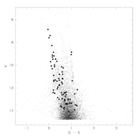
Figure 4: Colour-magnitude diagram for the Pegasus field with the location of variable stars shown as triangles.

Figure 5: Log period as a function of $J-H$ colour for each of the variable stars.

5.2 $\delta$ Scuti Stars

Due to the high time resolution of the WASP0 observations, the WASP0 data are particularly sensitive to very short period variations in stellar lightcurves. The best examples are the pulsating $\delta$ Scuti stars, of which 15 were identified from our observations. A number of the $\delta$ Scuti stars exhibit multi-periodic behaviour, such as stars 1 and 5. Stars 66 and 69 are also of the $\delta$ Scuti type but are multi-periodic and have been folded on the longer period. The bright star HD 207651 (star 69) is one of the two known variables to have been detected. Observations by Henry, Fekel, & Henry (2004) revealed this to be a triple system with the lower frequency variations resulting from ellipsoidal variations.

5.3 Eclipsing Binaries

Eclipsing binaries comprise at least 45% of the variables detected in this survey, and most of the unclassified variables are also strongly suspected to be eclipsing binaries. Most of the binaries are of the W Ursae Majoris (EW) type, the remainder being possible candidates for Algol (EA) or Beta Lyrae (EB) type binaries. The best example is star 47, for which exceptional data quality and clear phase coverage reveal slightly differing minima values, indicative of a close binary pair.

Of particular interest is star 57, an apparent eclipsing binary whose colour suggests a very late-type star. Although lack of phase information adds considerable uncertainty to the period, the estimated small period suggests that this may be an eclipsing system with M-dwarf components. There are only a few known eclipsing binaries of this type (Maceroni & Montalbán, 2004; Ribas, 2003) and they are very interesting as they allow rare opportunities to investigate the physical properties of late-type stars.

5.4 BY Draconis Stars

BY Draconis stars are generally spotted late-type stars whose variability arises from their rotation. Late-type stars comprise the minority of our variables list and so only 3 were identified as being of this type.

Star 74 has been classified as a BY Draconis due to the late spectral type and variable minima of the lightcurve. However, the lack of phase information and therefore uncertain period means that there are undoubtedly other equally viable classifications.

5.5 RR Lyrae Stars

The mean period of RR Lyrae stars is around 0.5 days and are therefore highly likely to be detected by the WASP0 observations. A total of 4 RR Lyrae stars were detected in this survey, one of which is a known RR Lyrae (star 54), the F0 star AV Peg. The remaining three consist of star 40 (type b), star 53 (type a), and star 58 (type c).

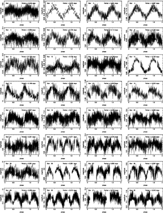
Figure 6: Variable stars 1–32 detected in the Pegasus field.

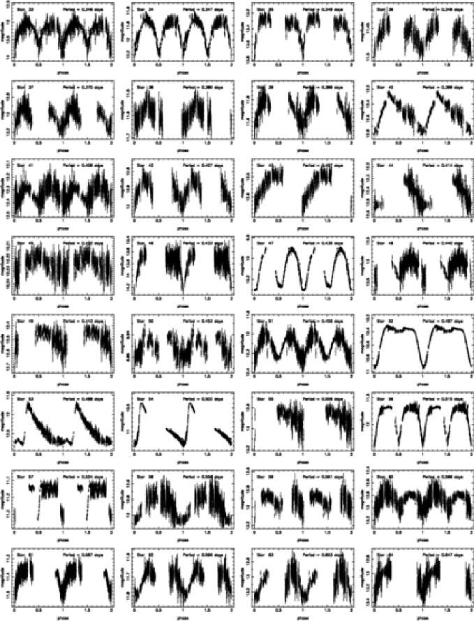
Figure 7: Variable stars 33–64 detected in the Pegasus field.

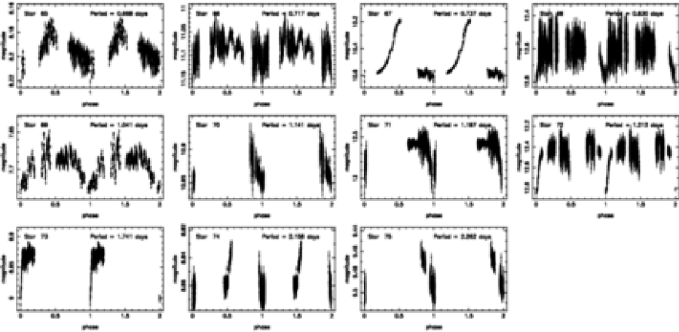
Figure 8: Variable stars 65–75 detected in the Pegasus field.

5.6 Unclassified and Suspected Variables

Around 24% of the detected variables were unable to be classified due to a lack of S/N and/or a lack of phase information. Examples of low S/N stars are stars 17–21. Stars 43-44 are examples of lightcurves missing valuable phase information. For some of these stars, the stellar image fell close to the edge of the chip and so was not observed consistently throughout the four nights. Star 65 has the shape, period, and colour (spectral type $\sim$ F0) of a typical RR Lyrae. However, the small amplitude of the variability is too small and so it remained unclassified. It is likely that many of the unclassified variables are eclipsing binaries for which one of the eclipses was not observed, as evidenced by their close proximity to the period-colour relationship visible in Figure 5.

6 Discussion

In total, $\sim 20000$ stars were searched for variability amongst the Pegasus field stars down to a magnitude of $\sim 13.5$. From these stars, 75 variable stars were positively identified. The techniques used to extract the variable stars from the data detected variability to an rms of around 0.6%. Hence, it is estimated that $\sim 0.4$% of Pegasus field stars brighter than $V\sim 13.5$ are variables with an amplitude greater than $\sim 0.6$%. For comparison, Hartman et al. (2004) used a similar instrument to observe a field in Cygnus and found that around 1.5% of stars exhibit variable behaviour with amplitudes greater than $\sim 3$%. Everett et al. (2002) detected variability in field stars for a much fainter magnitude range ($13.8<V<19.5$) and found the rate to be as high as 17%. However, as discussed earlier, the results presented here are likely to be biased towards lower periods due to the spacing of the observations. This also means that many long period variables may have remained undetected. Therefore the percentage of Pegasus field stars which exhibit variable behaviour calculated above should be considered a lower limit, as the actual value may well be slightly higher.

The Pegasus field stars surveyed in this study are predominantly solar-type stars. However, 60% of the variables detected are bluer than solar ($J-H<0.32$) with $\sim 30$% of these blue variables classified as $\delta$ Scuti stars. Those variables classified as “unknown” are fairly evenly distributed in colour and are most likely to be eclipsing binaries.

It has been noted by Everett et al. (2002) that low levels of stellar variability are likely to interfere with surveys hunting for transits due to extra-solar planets. Indeed it has developed into a major challenge for transit detection algorithms to distinguish between real planetary transits and false-alarms due to variables, especially grazing eclipsing binaries (Brown, 2003). If many of the unclassified variable stars from this survey are eclipsing binaries then these will account for well over half ($>40$) of the total variables found. This will have a significant impact upon transit surveys, especially wide-field surveys for which the stellar images are prone to under-sampling and therefore vulnerable to blending.

The radial velocity surveys have found that 0.5%–1% of Sun-like stars harbour a Jupiter-mass companion in a 0.05 AU (3–5 day) orbit (Lineweaver & Grether, 2003). Since approximately 10% of these planets with randomly oriented orbits will transit the face of their parent star, a suitable monitoring program of 20000 stars can be expected to yield $\sim 10$ transiting extra-solar planets. If we assume that the typical depth of a transit signature is similar to that of the OGLE transiting planets (Bouchy et al., 2004; Torres et al., 2004), then the photometric deviation for each transit from a constant lightcurve will be $<3$%. Figure 5 shows that many of the variables are of very low amplitude, with 20 having an rms of $<3$%. Hence, for the Pegasus field, the number of low amplitude variables detected outnumber the number of expected transits by a factor of 2:1. As previously mentioned, the number of variables detected by the WASP0 observations is relatively small compared to other similar studies of field stars. Thus, it can be expected that transit detection algorithms will suffer from large contamination effects due to variables, unless additional stellar attributes, such as colour, can be incorporated to reduce the false-alarm rate.

7 Conclusions

This paper has described observations of a field in Pegasus using the Wide Angle Search for Planets prototype. These observations were conducted from La Palma as part of a campaign to hunt for transiting extra-solar planets. Careful monitoring of stars in the Pegasus field detected 75 variable stars, 73 of which were previously unknown to be variable. It is estimated from these observations that $\sim 0.4$% of Pegasus field stars brighter than $V\sim 13.5$ are variables with an amplitude greater than $\sim 0.6$%. This is relatively low compared to other similar studies of field stars.

A concern for transiting extra-solar planet surveys is reducing the number of false-alarms which often arise from grazing eclipsing binaries and blended stars. It is estimated that the number of detectable transiting extra-solar planets one could expect from the stars monitored is a factor of two smaller than the number of variables with similar photometric amplitudes. Since the number of variables detected is relatively low, this has the potential to produce a strong false-alarm rate from transit detection algorithms.

Surveys such as this one are significantly improving our knowledge of stellar variability and the distribution of variable stars. It has been a considerable source of interest for many to discover the extent of sky that remains to be explored in this way, even to relatively shallow magnitude depths. It is expected that our knowledge of variable stars will continue to improve, particularly with instruments such as SuperWASP (Street et al., 2003) intensively monitoring even larger areas of sky.

References

- Alcock et al. (2003) Alcock C., et al., 2003, ApJ, 598, 597
- Bakos et al. (2002) Bakos, G.Á., Lázár, J., Papp, I., Sári, P., Green, E.M., 2002, PASP, 114, 974
- Bessell (1990) Bessell, M.S., 1990, PASP, 102, 1181
- Borucki et al. (2001) Borucki, W.J., Caldwell, D., Koch, D.G., Webster, L.D., Jenkins, J.M., Ninkov, Z., Showen, R., 2001, PASP, 113, 439
- Bouchy et al. (2004) Bouchy, F., Pont, F., Santos, N.C., Melo, C., Mayor, M., Queloz, D., Udry, S., 2004, A&A, 421, L13
- Brown (2003) Brown, T.M., 2003, ApJ, 593, L125
- Delfosse et al. (1998) Delfosse, X., Forveille, T., Mayor, M., Perrier, C., Naef, D., Queloz, D., 1998, A&A, 338, L67
- Derue et al. (2002) Derue, F., et al., 2002, A&A, 389, 149
- Everett et al. (2002) Everett, M.E., Howell, S.B., van Belle, G.T., Ciardi, D.R., 2002, PASP, 114, 656
- Hartman et al. (2004) Hartman, J.D., Bakos, G,., Stanek, K.Z., Noyes, R.W., 2004, AJ, 128, 1761
- Henry et al. (2004) Henry, G.W., Fekel, F.C., Henry, S.M., 2004, A&A, 127, 1720
- Høg et al. (2000) Høg, E., et al., 2000, A&A, 355, L27
- Kane et al. (2004) Kane, S.R., Collier Cameron, A., Horne, K., James, D., Lister, T.A., Pollacco, D.L., Street, R.A., Tsapras, Y., 2004, MNRAS, 353, 689
- Kidger (2004) Kidger, M.R., 2004, AJ, submitted
- Lineweaver & Grether (2003) Lineweaver, C.H., Grether, D., 2003, ApJ, 598, 1350
- Maceroni & Montalbán (2004) Maceroni, C., Montalbán, J., 2004, A&A, 426, 577
- Mochejska et al. (2002) Mochejska, B.J., Stanek, K.Z., Sasselov, D.D., Szentgyorgyi, A.H., 2002, AJ, 123, 3460
- Monet et al. (2003) Monet, D.G., et al., 2003, ApJ, 125, 984
- Ochsenbein et al. (2000) Ochsenbein, F., Bauer, P., Marcout, J., 2000, A&AS, 143, 23
- Press et al. (1992) Press, W.H., Teukolsky, S.A., Vetterling, W.T., Flannery, B.P., 1992, Numerical Recipes in FORTRAN: The Art of Scientific Computing (Cambridge University Press)
- Ribas (2003) Ribas, I., 2003, A&A, 398, 239
- Rubenstein (2001) Rubenstein, E.P., 2001, AJ, 121, 3219
- Street et al. (2002) Street, R.A., et al., 2002, MNRAS, 330, 737
- Street et al. (2003) Street, R.A., et al., 2003, MNRAS, 340, 1287
- Street et al. (2003) Street, R.A., et al., 2003, ASP Conf. Series, Vol. 294, Scientific Frontiers in Research on Extrasolar Planets, eds. D. Deming & S. Seager, p. 405
- Torres et al. (2004) Torres, G., Konacki, M., Sasselov, D.D., Jha, S., 2004, ApJ, 609, 1071
- Wenger et al. (2000) Wenger, M., et al., 2000, A&AS, 143, 9
- Woźniak et al. (2002) Woźniak, P.R., Udalski, A., Szymański, M., Kubiak, M., Pietrzyński, G., Soszyński, I., Żebruń, K., 2002, AcA, 52, 129
- Woźniak et al. (2004) Woźniak, P.R., et al., 2004, AJ, 127, 2436