Triggered massive-star formation
on the borders of Galactic H ii regions

We present SEST-SIMBA 1.2-mm continuum maps and ESO-NTT SOFI $JHK_{S}$ images of the Galactic H ii region RCW 79. The millimetre continuum data reveal the presence of massive fragments located in a dust emission ring surrounding the ionized gas. The two most massive fragments are diametrically opposite each other in the ring. The near-IR data, centred on the compact H ii region located at the south-eastern border of RCW 79, show the presence of an IR-bright cluster containing massive stars along with young stellar objects with near-IR excesses. A bright near- and mid-IR source is detected towards maser emissions, 1.2 pc north-east of the compact H ii region centre. Additional information, extracted from the Spitzer GLIMPSE survey, are used to discuss the nature of the bright IR sources observed towards RCW 79. Twelve luminous Class I sources are identified towards the most massive millimetre fragments. All these facts strongly indicate that the massive-star formation observed at the border of the H ii region RCW 79 has been triggered by its expansion, most probably by the collect and collapse process.

1 Introduction

Several physical processes linked to the expansion of H ii regions may trigger star formation. A review of the different processes is given by Elmegreen (elm98 (1998)). Among these processes, we are interested in the collect and collapse mechanism because it leads to the formation of massive objects (stars or clusters, Deharveng et al. deh05 (2005), hereafter paper I). This process, first proposed by Elmegreen & Lada (elm77 (1977)), has been treated analytically by Whitworth et al. (whi94 (1994)). Because of the supersonic expansion of an H ii region into the surrounding medium, a compressed layer of gas and dust accumulates between the ionization and the shock fronts. With time this layer grows in mass and possibly becomes gravitationally unstable, fragments, and forms massive cores. Those cores represent potential sites of second-generation massive-star formation.

To better understand this process of triggered massive-star formation, we have begun a multi-wavelength study of the borders of Galactic H ii regions. We selected H ii regions with a simple morphology (circular ionized regions surrounded by dust emission rings in the mid-IR) and hosting signposts of massive-star formation at their peripheries (luminous IR sources, ultracompact radio sources; see paper I for details about the selection criteria and the sample). Near-IR imaging gives information about the stellar nature of the luminous IR point sources observed at the borders of the ionized regions. It allows us to identify massive stars there and hence to confirm that massive objects (stars or clusters) are indeed formed via this process. Millimetre data (molecular emission lines or/and dust emission continuum) are used to search for massive fragments along an annular structure surrounding the ionized gas. The IR sources should be observed inside or close to these molecular cores. Sh 104, a Galactic H ii region, is the prototype of H ii regions experiencing the collect and collapse process to form massive stars (Deharveng et al. deh03 (2003)). Other candidates proposed in paper I are under analysis; RCW 79 is one of these. It has been studied in detail by Cohen et al. (coh02 (2002)). The presence of a compact H ii region located at its south-east border, just behind its ionization front, indicates that massive-star formation has taken place there. Cohen et al. proposed that RCW 79 encountered a massive molecular clump during its expansion, triggering star formation there (see the end of their sect. 5). We present in this paper new observational facts, based on near-IR, mid-IR and millimetre continuum data, that support the hypothesis of the collect and collapse mechanism being at work there. Sect. 2 introduces the RCW 79 region. Observations and data reduction are presented in Sect. 3. The results are presented in Sect. 4 and are discussed in Sect. 5. Our conclusions are given in Sect. 6.

2 Presentation of RCW 79

RCW 79 (Rodgers, Campbell and Whiteoak rod60 (1960), $l$=308$.\!\!^{\circ}$6, $b$=0$.\!\!^{\circ}$6) is a bright optical H ii region of diameter $\sim$12^′, located at a distance of 4.3 kpc (Russeil rus03 (2003)). This region and its surroundings have been studied by Cohen et al. (coh02 (2002)), hereafter CGPMC. CGPMC present a 843 MHz continuum emission map showing a shell nebula, corresponding to the optical H ii region, and a compact H ii region, without any optical counterpart, at the south-east border of the nebula’s shell. The velocity of the ionized gas is in the $-40$ to $-51$ km s^-1 range (see Sect. 4.3).

RCW 79 is nearly completely surrounded by a dust ring (see Fig. 1), revealed by its mid-IR emission in the MSX Band A (centred at 8.3 $\mu$m, Price et al. pri01 (2001)) and in the Spitzer IRAC (Fazio et al. faz04 (2004)) channel 4 (centered at 8 $\mu$m, GLIMPSE survey, Benjamin et al. ben03 (2003)). In the hot photodissociation regions (PDRs) surrounding H ii regions, the emission in the MSX Band A and in IRAC (channel 4 is dominated by emission bands centred at 7.7 and 8.6 $\mu$m and commonly attributed to polycyclic aromatic hydrocarbon-like molecules, PAHs; Léger & Puget leg84 (1984)). Fig. 1 presents a colour composite image of this region. The H$\alpha$ emission of the ionized gas (from the SuperCOSMOS H-alpha survey, Parker & Phillips par98 (1998)) appears in turquoise. The dust emission (image from the Spitzer GLIMPSE survey) in the band centered at 8 $\mu$m appears in orange. These two emissions are clearly anti-correlated. PAHs are destroyed in the ionized region, but are present in the photo-dissociated region, where they are excited by the photons leaking from the H ii region.

Table 1: Coordinates of objects discussed in the text

Object	$\alpha_{2000}$	$\delta_{2000}$
Centre of RCW 79	13h 40m 17$.\!\!^{\rm s}$0	$-$61∘ 44′ 00′′
IRAS 13374$-$6130	13h 40m 53$.\!\!^{\rm s}$2	$-$61∘ 45′ 47′′
MSX point source	13h 40m 53$.\!\!^{\rm s}$1	$-$61∘ 45′ 51′′
Centre of the compact H ii region1	13h 40m 52$.\!\!^{\rm s}$5	$-$61∘ 45′ 54′′
Maser sources	13h 40m 57$.\!\!^{\rm s}$6	$-$61∘ 45′ 43′′

¹ Not given in CGPMC. Measured from their figs. 3 and 5 (about 5^′′  accuracy)

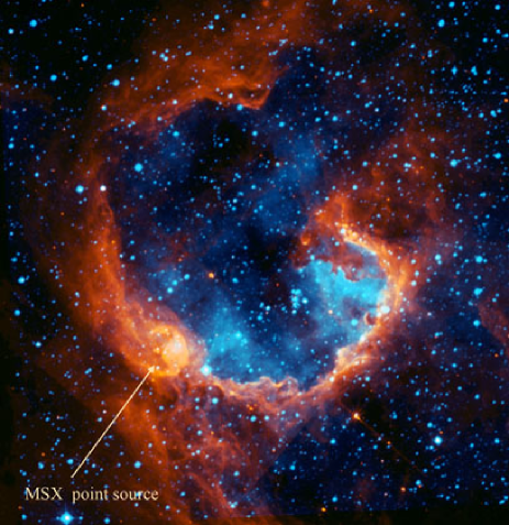
Figure 1: Spitzer-IRAC 8 $\mu$m image from the GLIMPSE survey (orange) superimposed on a SuperCOSMOS H$\alpha$ image (turquoise) of RCW 79. The location of the MSX point source is indicated. The field size is 15^′$\times$15^′

Table 1 gives the position of sources discussed in the text. The IR source G308.7452+00.5482 in the MSX Point Source Catalog (Egan et al. ega99 (1999)) lies in the direction of the dust ring, towards the compact H ii region at the south-eastern border of RCW 79 (see Fig. 1). This point source also corresponds to IRAS 13374$-$6130. It has the luminosity (55000 $L_{\hbox{$\odot$}}$) and colours of a UC H ii region (CGPMC, paper I). The high angular resolution of the GLIMPSE survey allows us to resolve the MSX point source. Fig. 1 shows that it is composed of several compact components surrounded by a small dust emission ring of diameter $1\hbox{$.\mkern-4.0mu^{\prime}$}7$. The compact H ii region is not seen on the H$\alpha$ image, indicating a high visual extinction in this direction. The near-IR data presented in this paper focus on this compact H ii region where they unveil the presence of a small cluster.

RCW 79 belongs to a molecular complex, in Centaurus, studied by Saito et al. (sai01 (2001)) using the NANTEN telescope (see their figs. 1a and 4). The ¹²CO (1–0) emission, integrated over the velocity range $-64$ to $-36$ km s^-1, shows three condensations at the borders of RCW 79. The C¹⁸O (1–0) emission integrated over the $-$50 to $-$44 km s^-1 range shows a massive condensation ($M\simeq 6000$–$12000M_{\odot}$) in the direction of the compact H ii region. The mean H₂ density in this condensation is 1400 cm^-3.

Maser emissions (OH, methanol and water) have been detected in RCW 79 towards the mid-IR MSX point source (Caswell cas04 (2004), van der Walt et al. van95 (1995); see also Table 1), indicating that massive-star formation is taking place. The emission peak of the methanol and water masers are observed at $-51$ and $-$49 km s^-1, respectively, indicating that those emissions are indeed associated with RCW 79.

Fig. 1 shows a hole in the ring of dust emission surrounding RCW 79, to the north-west. H$\alpha$ emission is observed in this direction, suggesting that RCW 79 may be experiencing a champagne phase, the ionized gas flowing away from the H ii region through this hole. We discuss this point in Sect. 4.3.

2.1 Radio continuum emission

The MGPS2 (Green gre99 (1999)) 843 MHz radio continuum map presented by CGPMC (their fig. 5), obtained with a resolution of $43\hbox{${}^{\prime\prime}$}\times 49\hbox{${}^{\prime\prime}$}$, shows that the radio source corresponding to RCW 79 consists of a large shell nebula, of diameter $\sim 12\hbox{${}^{\prime}$}$ (similar to the optical nebula), and a compact region. No flux density has been published for this source. From the map we estimate that its flux density is about 1/16 that of the total source. Assuming that we are dealing with thermal emission, and adopting the total flux density of the source, 17 Jy at 5 GHz, measured by Caswell & Haynes (cas87 (1987)), we obtain fluxes of 1 Jy and 16 Jy respectively for the compact and extended radio sources.

These radio flux densities allow us to estimate the ionizing-photon fluxes, and hence the spectral types of the main exciting stars (assuming that a single main-sequence star dominates the ionization in each region). Using eq. 1 of Simpson & Rubin (sim90 (1990)), and a distance of 4.3 kpc, we derive ionizing fluxes $N_{\mathrm{Lyc}}$ of $2.9\times 10^{49}$ and $1.9\times 10^{48}$ photons s^-1 for the extended and the compact H ii regions, respectively. There are large uncertainties in the effective temperatures and the ionizing fluxes of massive stars, for a given spectral type. According to Vacca et al. (vac96 (1996)) and to Schaerer & de Koter (sch97 (1997)), these ionizing fluxes correspond to O5V and O9.5V stars, respectively. According to Smith et al. (smi02 (2002)), these fluxes correspond to O3V–O4V and O8.5V stars, respectively. According to Martins et al. (mar05 (2005)) they indicate O4V and O8V stars. Thus the large RCW 79 H ii region is a high-excitation region possibly ionized by a star in the O3V–O5V range, while the compact H ii region is of lower excitation, possibly ionized by a star of spectral type O8V–O9.5V. On the other hand, the IR luminosity of the IRAS point source observed in the direction of the compact H ii region (55000 $L_{\odot}$) gives a limit of O9V for the most luminous/massive star of the exciting cluster. New radio continuum maps at higher resolution are needed to resolve the compact H ii region and measure its size and radio flux.

3 Observations

3.1 SEST-SIMBA 1.2-millimetre continuum imaging

Continuum maps at 1.2-mm (250 GHz) of a 20^′$\times$ 20^′  field centred on RCW 79 have been obtained using the 37 channel SIMBA bolometer array (SEST Imaging Bolometer Array) mounted at SEST on May 7-8 2003. The beam size is 24^′′. Nine individuals maps covering the whole region were obtained with the fast scanning speed (80^′′per second). The total integration time was 10.5 hours. The final map was constructed by combining the individual maps. Skydips were performed after each integration to determine the atmospheric opacity. Maps of Uranus and Neptune were obtained for the calibration. The individual maps were reduced and analyzed using MOPSIC, a software package developed by Robert Zylka (Grenoble Observatory ; see also http://www.astro.ruhr-uni-bochum.de/nielbock/simba/mopsic.pdf). The common procedures are described in Chapter 4 of the SIMBA Observers Handbook. A detailed description of the data reduction can be found in Chini et al. (chi03 (2003)).

The data reduction of the nine individual maps is done in two steps. The first step includes a global baseline fit, despiking, deconvolution of the instrumental bandpass, gain-elevation, opacity corrections and skynoise reduction. A map is then created by combination of individual maps. This map is used to define a polygon that includes the emission zone. Then the same procedure is applied to the original FITS files but using the zone outside the polygon for the baseline fitting. The final map is obtained at the end of this second iteration. The calibration was obtained using planet maps. We derived a conversion factor of 55 mJy/count for the first day and 51 mJy/count for the second day, applied respectively to the individual maps before the final combining. The residual noise in the final map is about 20 mJy/beam (1$\sigma$). We then used the emission above 5$\sigma$ (100 mJy/beam level) to define the 1.2-mm condensations.

3.2 ESO-NTT near-IR imaging

Images in the $J$ (1.25 $\mu$m), $H$ (1.65 $\mu$m), and $K_{S}$ (2.2 $\mu$m) near-infrared bands were obtained on the nights of 14 and 15 February 2003 with the SofI camera at the ESO New Technology Telescope (NTT). They cover a $2\hbox{$.\mkern-4.0mu^{\prime}$}66\times 3\hbox{$.\mkern-4.0mu^{\prime}$}85$ area centered on the bright MSX point source. The corresponding images obtained on the first night combined 40 ($J$), 19 ($H$), and 10 ($K_{S}$) separate frames obtained with small offsets in between, using stellar images to determine the telescope offsets before combination. Each frame consisted in turn of 20 individual exposures co-added on the detector, with individual integration times of 2.4, 2.4, and 1.2 sec in the $J$, $H$ and $K_{S}$ filters. The rather short detector integration times were chosen because of the presence of bright saturating stars in the field of view. The observation sequence was repeated on the following night, this time obtaining respectively 26, 24, and 8 frames with 15 individual exposures of 4, 2.5, and 2 sec. The individual images were dark-subtracted, divided by a master flat field, and sky-subtracted before combination. Both the amplitude of the telescope offset pattern and the number of exposures in each filter were large enough to allow us to produce an acceptable sky frame by median averaging the dark-subtracted, flat-fielded frames uncorrected for the telescope motion, clipping off in the median averaging the upper half of the pixel values at each detector position.

Sources were detected using DAOFIND (Stetson ste87 (1987)). A master list of sources was produced by running DAOPHOT on a single image built by adding the $J$, $H$, and $K_{S}$ images, so as to ensure that all sources observed in at least one filter entered this master list. Unsaturated and relatively isolated bright stars in the co-added $JHK_{S}$ image were used to determine an approximate PSF, needed for automated point source identification. Photometry was then performed on the images obtained through each filter by defining an undersized aperture at the position of each star in the master list, measuring the flux inside it, and adding the rest of the flux in the PSF as given by the fit of a circularly symmetric radial profile to each stellar image. This procedure allowed both to reduce the contamination to the aperture photometry by other stars located on the wings of the PSF, and to adjust to the mildly variable image quality across the field of view. Finally, zero-point calibration was carried out by observing six infrared standard stars from Persson et al. (per98 (1998)) at different air-masses during both nights.

3.3 H$\alpha$ observations

H$\alpha$ Fabry-Perot observations of RCW 79 were obtained with the CIGALE instrument on a 36-cm telescope (La Silla, ESO) in May 1990. A description of the instrument, including data acquisition and reduction techniques, can be found in le Coarer et al. (lec92 (1992)). The field of view is 39^′ with a pixel size of 9^′′. The Fabry-Perot interferometer has an interference order of 2604 at H$\alpha$, providing a free spectral range equivalent to 115 km s^-1, and a spectral sampling of 5  km s^-1. The velocity accuracy is $\sim$1 km s^-1.

The H$\alpha$ profiles are decomposed into several components: H$\alpha$ geocoronal and OH night-sky lines, and nebular lines. The channel maps show that the nebular velocity ranges from $-$72 km s^-1 to $-$18 km s^-1. The H$\alpha$ emission associated with RCW 79 is in the range $-$51 to $-$40 km s^-1. Two other H$\alpha$ emissions are superimposed along the line of sight: the local arm emission at V${}_{LSR}\sim 0$ km s^-1, and that of the Sagittarius arm at V${}_{LSR}\sim-25$ km s^-1. To increase the S/N ratio, profiles were binned over 5 pixel$\times$5 pixel areas.

4 Results

4.1 Continuum imaging at 1.2-mm

Figure 2 shows the 1.2-mm continuum emission superimposed on a SuperCOSMOS H$\alpha$ image of the region.

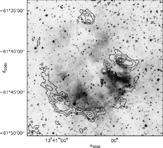
Figure 2: Millimetre continuum emission (contours) superimposed on a SuperCOSMOS H$\alpha$ image of the region. The first levels are 50, 100 and 150 and then increase in steps of 100 mJy/beam, from 300 to 700 mJy/beam

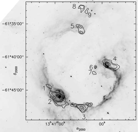
Figure 3: Millimetre continuum emission (contours) superimposed on the GLIMPSE 8 $\mu$m image of the region. The levels are 100, 150 mJy/beam and then increase from 300 to 700 mJy/beam in steps of 100 mJy/beam. The condensations discussed in the text are identified by their numbers (from 1 to 9). Their limits, used for the mass derivations, are defined by the 100 mJy/beam contour (5$\sigma$ level, see text)

The fact that this 1.2-mm emission surrounds the ionized region, is located just beyond the ionization front (Fig. 2) and shows the same annular structure as shown by the mid-IR dust emission (Figs. 1 and 3) demonstrates that this emission is associated with RCW 79. Fig. 3 presents the 1.2-mm continuum emission (as contours) superimposed on the 8 $\mu$m GLIMPSE image of RCW 79. The lowest contour shown in Fig. 3 delineates the condensations’ surface as defined, for the mass estimates, at the 5$\sigma$ level (100 mJy/beam, Sect. 3.1).

The millimetre continuum map reveals the presence of nine fragments. Five (nos 1 to 5) of the nine form an emission ring surrounding the main ionized region RCW 79. Two (nos 6 and 7) are situated in front of the ionized gas, as shown by the absorption features observed in the visible (Fig. 2). Fragments 8 and 9, in the North, are most probably related to the region, judging from the faint GLIMPSE mid-IR emission observed there.

4.1.1 Mass estimates

The millimetre continuum emission from condensations identified in Fig. 3 is mainly due to optically thin thermal dust emission. Following Hildebrand (hil83 (1983)) and assuming standard dust properties and gas-to-dust ratio, the integrated millimetre flux is related to the total (gas+dust) mass of the condensations. For the mass estimates, we used the 1.2-mm integrated fluxes, $F^{\mathrm{int}}_{\mathrm{1.2mm}}$, given in Table LABEL:massemm. For condensation 2, we did not correct this flux for the free-free emission of the compact H ii region. Indeed, this emission does not coincide with the millimetre emission peak, and higher resolution radio data are needed to accurately estimate its contribution. Note that the dust mass estimate for this condensation is, therefore, an upper limit.

According to Hildebrand (hil83 (1983)) the “millimetre” (gas+dust) mass is related to the flux by

$$M_{\mathrm{(gas+dust)}}\,(M_{\odot})=g\,\,\frac{F^{\mathrm{int}}_{\mathrm{1.2mm}}(\mathrm{Jy})\,\,(D\,(\mathrm{kpc}))^{2}}{\kappa_{\mathrm{1.2mm}}\,\,B_{\mathrm{1.2mm}}(T_{\mathrm{dust}})},$$

where $\kappa_{\mathrm{1.2mm}}$ is the dust opacity per unit mass at 1.2-mm and $B_{\mathrm{1.2mm}}(T_{\mathrm{dust}})$ the Planck function for a temperature $T_{\mathrm{dust}}$. The values of $T_{\mathrm{dust}}$ and $\kappa_{\mathrm{1.2mm}}$ are unknown and have to be assumed to derive the masses. The dust temperature should be in the 20–30 K range, as usually assumed for protostellar condensations (cf. Motte et al. mot03 (2003)). Ossenkopf & Henning (oss94 (1994)) recommended using a value of $\kappa_{\mathrm{1.2mm}}$ = 1 cm² g^-1 for a protostellar cores dust mass and $g$ is the gas-to-dust ratio that we assume to be 100. Table LABEL:massemm lists the measured and derived properties obtained for the millimetre fragments identified in Fig. 3. Column 1 gives the fragment numbers, columns 2 and 3 give the emission peak coordinates, column 4 gives the 1.2-mm integrated flux, and column 5 the range of derived masses for the corresponding fragment, depending on the adopted temperature (20 or 30 K). Note that the lower mass values correspond to the higher dust temperature.

Table 2: Mass estimates for the millimetre fragments

Number	Peak position		$F^{\mathrm{int}}_{\mathrm{1.2mm}}$1	Mass range2
	$\alpha_{2000}$	$\delta_{2000}$	(mJy)	($M_{\odot}$)
1	13h 40m 56$.\!\!^{\rm s}$00	$-$61∘ 45′ 51$.\!\!^{\prime\prime}$75	224	42 – 70
2	13h 41m 09$.\!\!^{\rm s}$30	$-$61∘ 44′ 22$.\!\!^{\prime\prime}$76	4200	796 – 13263
3	13h 40m 25$.\!\!^{\rm s}$45	$-$61∘ 47′ 43$.\!\!^{\prime\prime}$68	2350	444 – 742
4	13h 39m 54$.\!\!^{\rm s}$00	$-$61∘ 41′ 04$.\!\!^{\prime\prime}$22	3000	567 – 947
5	13h 40m 26$.\!\!^{\rm s}$75	$-$61∘ 36′ 16$.\!\!^{\prime\prime}$10	795	150 – 251
6	13h 40m 08$.\!\!^{\rm s}$11	$-$61∘ 41′ 27$.\!\!^{\prime\prime}$87	81	15 – 25
7	13h 40m 10$.\!\!^{\rm s}$58	$-$61∘ 42′ 23$.\!\!^{\prime\prime}$85	144	27 – 45
8	13h 40m 25$.\!\!^{\rm s}$10	$-$61∘ 32′ 27$.\!\!^{\prime\prime}$05	483	91 – 153
9	13h 40m 19$.\!\!^{\rm s}$90	$-$61∘ 33′ 13$.\!\!^{\prime\prime}$40	173	33 – 55

¹ 1.2-mm flux integrated above the 5$\sigma$ level
² Mass calculations performed with $T_{\rm{dust}}$=30 and 20 K for the lower and higher values, respectively
³ Upper limit (see text)

4.2 Stellar content of the millimetre condensations

We have investigated the stellar content of the three most massive millimetre condensations (nos 2, 3 and 4, see Fig. 3). We are particularly interested in identifying red and luminous objects observed in the direction of these condensations. Such sources may represent embedded massive young stellar objects, whose formation has been triggered by the expansion of the RCW 79 H ii region. We look in more detail at condensation 2 where the stellar cluster ionizing the compact H ii region is observed. The near-IR ESO-NTT observations cover this region.

Figs. 4, 5, and 6 (top) present the 1.2-mm emission as contours superimposed on the Spitzer GLIMPSE 3.6 $\mu$m frame for condensations 2, 3 and 4, respectively. Several of the objects discussed in the text are identified according to their numbers in Table 3. Figs. 4, 5, and 6 (bottom) present a colour composite image displaying the 2MASS $K_{S}$ frame in blue, the GLIMPSE 3.6 $\mu$m frame in green and the GLIMPSE 8 $\mu$m frame in red, for condensations 2, 3 and 4, respectively. Note that the 3.6 and 8 $\mu$m images are very similar, both filters including PAH emission bands (at 3.3 and 8.6 $\mu$m). However, the continuum emission from normal stars is only visible in the 3.6 $\mu$m image and not at 8 $\mu$m, hence a dominance of the $K_{S}$ (blue) and 3.6 $\mu$m (green) emissions from normal stars in Figs. 4, 5, and 6 (bottom).

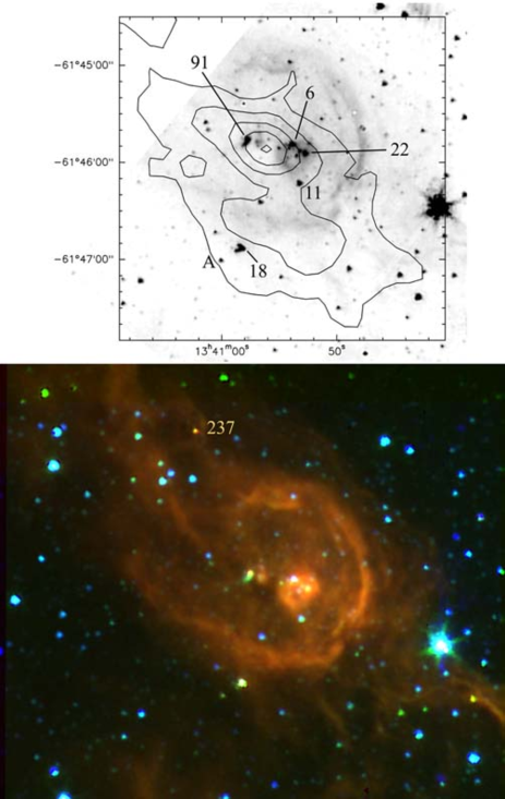
Figure 4: Condensation 2 - Top) The 1.2-mm continuum emission is superimposed, in contours, on the 3.6 $\mu$m image taken from the Spitzer GLIMPSE survey. Bottom) Color composite image combining the $K_{S}$ image from the 2MASS survey (in blue), and the 3.6 $\mu$m (in green) and the 8 $\mu$m (in red), both from the GLIMPSE survey. The stars discussed in the text are identified by their numbers in Table 3

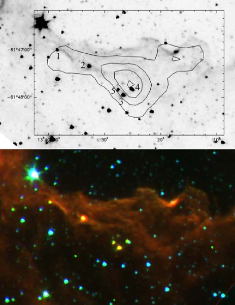
Figure 5: As Fig. 4 but for condensation 3

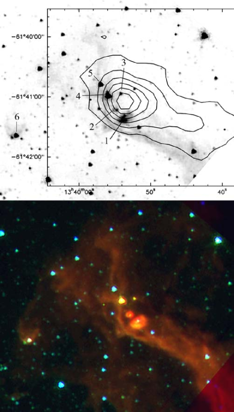
Figure 6: As Fig. 4 but for condensation 4

Table 3 gives the position and photometry from 1.25 $\mu$m to 8 $\mu$m of the sources discussed in the following. Column 1 gives their identification numbers, according to Figs. 4 (see also Fig. 11), 5, and 6, for condensations 2, 3 and 4, respectively. Columns 2 and 3 give their coordinates according to the GLIMPSE point source catalogue (PSC, http://www.astro.wisc.edu/sirtf/), except for sources in condensation 2 for which the ESO-NTT positions - more accurate - have been taken. For the star of source 1 in condensation 4 (1 star in Table 3) we have taken the 2MASS position. Columns 4 to 6 gives their $J$, $H$ and $K_{S}$ magnitudes, from the ESO-NTT observations for sources near condensation 2, and from the 2MASS PSC (http://tdc-www.harvard.edu/software/catalogs/tmpsc.html) for sources near condensations 3 and 4. Columns 7 to 10 gives their [3.6], [4.5], [5.8] and [8.0] magnitudes from the GLIMPSE PSC. When not available from the PSC, GLIMPSE magnitudes have been measured (aperture photometry) using the Basic Calibrated Data frames. Those measurements are indicated with asterisks in Table 3.

Table 3: Magnitudes of sources associated with the 1.2-millimetre condensations 2, 3 and 4

Object	$\alpha_{2000}$	$\delta_{2000}$	$J$	$H$	$K_{S}$	[3.6]	[4.5]	[5.8]	[8.0]	Comments
Condensation 2
Cluster
6	13h 40m 53$.\!\!^{\rm s}$8	$-$61∘ 45′ 46′′	13.17	11.71	10.81					MS star, $A_{V}$=15 mag
11	13h 40m 53$.\!\!^{\rm s}$1	$-$61∘ 46′ 11′′	16.05	12.69	10.94	9.75	9.77	9.41		Giant, $A_{V}$=23 mag
15	13h 40m 54$.\!\!^{\rm s}$3	$-$61∘ 45′ 47′′	12.70	12.48	12.25					MS star, $A_{V}$=3 mag
19	13h 40m 53$.\!\!^{\rm s}$3	$-$61∘ 45′ 53′′	13.30	12.60	12.21					MS star, $A_{V}$=7 mag
22	13h 40m 52$.\!\!^{\rm s}$5	$-$61∘ 45′ 52′′	13.55	12.73	12.16					MS star, $A_{V}$=9 mag
46	13h 40m 53$.\!\!^{\rm s}$5	$-$61∘ 45′ 47′′	15.19	13.68	12.87					MS star, $A_{V}$=14.5 mag
85	13h 40m 54$.\!\!^{\rm s}$9	$-$61∘ 45′ 48′′	16.99	14.85	13.35					MS star, $A_{V}$=22 mag
136	13h 40m 53$.\!\!^{\rm s}$1	$-$61∘ 45′ 51′′	16.53	14.61	13.60					MS star, $A_{V}$=18 mag
154	13h 40m 54$.\!\!^{\rm s}$0	$-$61∘ 45′ 49′′	18.22	16.27	13.98					Near-IR excess
372	13h 40m 54$.\!\!^{\rm s}$4	$-$61∘ 45′ 50′′	19.02	17.44	15.49					Near-IR excess
Whole cluster	13h 40m 53$.\!\!^{\rm s}$4	$-$61∘ 45′ 53′′				7.35∗	7.21∗	4.74∗	2.74∗
237	13h 41m 02$.\!\!^{\rm s}$3	$-$61∘ 44′ 16′′	17.41	15.79	14.23	10.64	8.56	7.79	6.08	Near-IR excess
Filament
31	13h 40m 56$.\!\!^{\rm s}$6	-61∘ 45′ 39′′	13.56	13.34	12.96	12.49	12.60
54	13h 40m 56$.\!\!^{\rm s}$8	-61∘ 45′ 45′′	14.76	13.89	13.09
91	13h 40m 57$.\!\!^{\rm s}$6	-61∘ 45′ 44′′	16.62	14.45	12.59	8.66∗	7.60∗	7.25	6.18	Maser position
460	13h 40m 57$.\!\!^{\rm s}$9	-61∘ 45′ 42′′	17.57	15.72	14.49
482	13h 40m 58$.\!\!^{\rm s}$2	-61∘ 45′ 45′′	16.61	15.35	14.05
Red objects
18	13h 40m 58$.\!\!^{\rm s}$3	-61∘ 46′ 50′′	17.11	13.83	11.45	8.47	7.54	6.79	5.85	Near-IR excess
89	13h 40m 58$.\!\!^{\rm s}$7	-61∘ 46′ 52′′	18.58	15.35	13.34	10.83	10.71			Giant?
186	13h 40m 58$.\!\!^{\rm s}$5	-61∘ 46′ 48′′	18.96	15.86	13.91					Giant?
A	13h 41m 00$.\!\!^{\rm s}$0	-61∘ 46′ 58′′	$\geq$ 19.5	16.80	14.21	10.95	9.81	8.72	7.84	Not detected in $J$
101	13h 40m 59$.\!\!^{\rm s}$0	-61∘ 46′ 50′′	17.85	14.91	13.64					Giant
Giants
2	13h 41m 04$.\!\!^{\rm s}$5	-61∘ 44′ 41′′	11.78	10.60	10.15	9.82	10.03	10.03
4	13h 41m 02$.\!\!^{\rm s}$6	-61∘ 44′ 45′′	13.07	11.08	10.13	9.50	9.60	9.41	9.71
7	13h 41m 05$.\!\!^{\rm s}$2	-61∘ 44′ 46′′	16.11	12.262	10.28	8.87	8.88	8.59	8.49
28	13h 41m 05$.\!\!^{\rm s}$3	-61∘ 44′ 35′′	17.19	13.71	11.91	10.60	10.67
37	13h 41m 05$.\!\!^{\rm s}$4	-61∘ 44′ 59′′	16.66	13.77	12.30	11.30	11.23	11.54
Condensation 3
1	13h 40m 38$\hbox{$.\!\!^{\rm s}$}3$	$-$61∘ 47′ 00′′	16.39	15.81	14.83	9.73	8.61	7.62	6.79	Near-IR excess
2	13h 40m 32$.\!\!^{\rm s}$65	$-$61∘ 47′ 20′′	14.08	12.79	11.82	9.43	9.03	6.76	4.95	Near-IR excess
3	13h 40m 26$.\!\!^{\rm s}$6	$-$61∘ 47′ 56′′	17.24	14.32	12.57	9.55	7.15	5.89	5.29
4	13h 40m 25$.\!\!^{\rm s}$2	$-$61∘ 47′ 48′′	15.50	12.48	11.12	9.03	7.85	7.05	7.03	Giant
5	13h 40m 27$.\!\!^{\rm s}$5	$-$61∘ 47′ 50′′	15.64	14.21	13.14	9.80	8.67	7.84	7.41	Near-IR excess
Condensation 4
1 nebula	13h 39m 53$\hbox{$.\!\!^{\rm s}$}6$	$-$61∘ 41′ 21′′				8.19∗	7.94∗	5.09∗	3.41∗
1 star	13h 39m 53$.\!\!^{\rm s}$68	$-$61∘ 41′ 19$.\!\!^{\prime\prime}$2	12.19	11.45	11.01
2	13h 39m 54$.\!\!^{\rm s}$7	$-$61∘ 41′ 13′′	14.86	14.53	14.25	10.90	9.69	7.15	5.28
3	13h 39m 54$.\!\!^{\rm s}$2	$-$61∘ 40′ 57′′	16.11	14.86	14.24	10.32	9.02	7.83	6.72
4	13h 39m 55$.\!\!^{\rm s}$9	$-$61∘ 40′ 58′′	14.68	13.54	10.62	7.19	6.22∗	5.40	4.69	Near-IR excess
5	13h 39m 57$.\!\!^{\rm s}$1	$-$61∘ 40′ 47′′	13.87	10.59	9.01	7.80	8.02	7.62	7.62	Giant
6	13h 40m 08$.\!\!^{\rm s}$9	$-$61∘ 41′ 38′′	13.91	11.96	10.29	8.72	8.18	7.51	6.38	Near-IR excess

^∗ Magnitude obtained by aperture photometry (see text)

We use both near- and mid-IR data to discuss the nature of the sources observed towards the condensations. We present the $K_{S}$ versus $J-K_{S}$, $J-H$ versus $H-K_{S}$ and the [3.6]$-$[4.5] versus the [5.8]$-$[8.0] diagrams of the stars observed towards condensations 2, 3 and 4 in Figs. 7, 8 and 9, respectively. The sources are identified in Figs. 7, 8 and 9 as their number in Table 3 at which we attached C3 or C4 for labeling the objects of condensation 3 and 4, respectively. For the main sequence in Fig. 7 and 8, we have used the absolute magnitudes $M_{V}$ of stars from O3 to O9 of Martins et al. (mar05 (2005)) and from Schmidt-Kaler (sch82 (1982)) for later type stars. The colours for main sequence stars and the colours and absolute magnitudes for giants are from Koornneef (koo83 (1983)). Note that large differences exist in the estimated absolute visual magnitudes of massive stars, depending on the authors. As an example we display in Fig. 7 the uncertainties for an O6V star. The absolute magnitude of such a star is $-$5.5 according to Schmidt-Kaler, $-$5.11 according to Vacca et al. (vac96 (1996)) and $-$4.92 according to Martins et al. (mar05 (2005)). Recent results on ISO-SWS data dealing with ionization diagnostics of compact H ii regions (Morisset et al. mor04 (2004)) indicate that the model used by Martins et al. gives better agreement with the observations. Therefore we adopt this calibration in the following. Typical errors are 0.04 for the $K_{S}$ magnitudes and 0.07 for the $J-H$ and $H-K_{S}$ colours. The reddening law is from Mathis (mat90 (1990)) for $R_{V}$=3.1. In both diagrams we have drawn the interstellar reddening line originating from a B2V star and from a MOIII star, for $A_{V}$=30 mag. In Fig 7, we also plot the main sequence shifted by a visual extinction of $A_{V}$=4.3 mag using the standard value of $A_{V}$=1 mag kpc^-1 for the foreground interstellar reddening.

We are interested in detecting massive young stellar objects and candidates ionizing stars. Therefore we identify, in Fig. 7, all the sources that have a $K_{S}$ magnitude brighter than that corresponding to a B2V star. However, giants also fall in this group and the magnitude-colour diagram alone does not allow one to separate those stars from the others. Therefore we use the colour-colour diagrams (Figs. 8 and 9), which clearly separates giants from other sources.

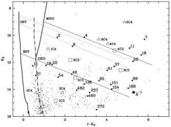
Figure 7: Magnitude-colour diagram for the sources observed towards condensations 2, 3 and 4. The thick solid curves show the main sequence (class V) and the sequence of giants (class III) for a distance of 4.3 kpc and no extinction. The thick dash-dotted curve shows the main sequence with a foreground visual extinction of 4.3 mag (see text). The two solid lines are the reddening lines for 30 mag of visual extinction for a B2V star and an M0III star. The thin dotted lines indicate the extreme values for the absolute magnitude of an O6V star with reddening lines corresponding to 30 mag of visual extinction

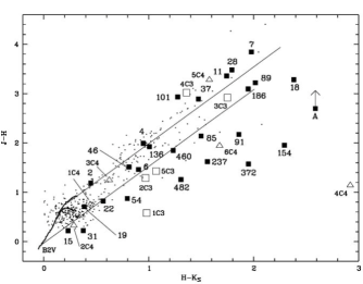
Figure 8: Colour-colour diagram for sources observed towards condensations 2, 3 and 4. The two curves show the main sequence (class V) and the sequence of giants (class III) for a distance of 4.3 kpc and no extinction. The parallel lines are the reddening lines for 30 mag of visual extinction for a B2V star (lower) and an M0III star (upper)

Fig. 9 presents the GLIMPSE colour-colour diagram for the sources of Table 3 and for all the sources observed in the direction of the RCW 79 field, extracted from the GLIMPSE PSC. The locations of Class I sources (SED dominated by emission from an envelope), Class II sources (SED dominated by emission from a disk), and giants are taken from Allen et al. (all04 (2004)) and Whitney et al. (whi04 (2004)). The $[3.6]-[4.5]$ versus $[5.8]-[8.0]$ diagram is a useful tool for identifying young sources in different evolutionary stages. The geometry of the source and the temperature of the central object deeply influence its location in this diagram (see Whitney et al. whi04 (2004)). Two extinction vectors are shown in Fig. 9 for $A_{V}$=30 mag, taken from Allen et al. (all04 (2004)), using the two extremes of six vectors calculated by Megeath et al. (meg04 (2004)). Extinction tends to move sources to the upper left (see Fig. 9). We have also indicated in Fig. 9 the colours of the filaments (filled lozenge) measured in the direction of the PDR surrounding the ionized gas, and probably dominated by the PAH emission bands in the 3.6 $\mu$m, 5.8 $\mu$m and 8.0 $\mu$m filters. These colours are $[3.6]-[4.5]\simeq$0.1 and $[5.8]-[8.0]\simeq$1.8.

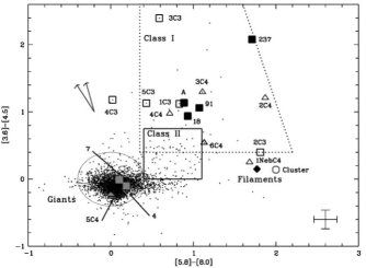
Figure 9: GLIMPSE colour-colour diagram, [3.6]$-$[4.5] versus [5.8]$-$[8.0], for the sources observed towards the most massive condensations detected at 1.2-mm (nos 2, 3 and 4) and the sources observed in the RCW 79 field (small black dots), extracted from the GLIMPSE PSC. The sources observed towards the compact H ii region are identified by their numbers in Table 3 and shown as filled squares. The sources observed towards condensation 3 are shown as empty squares and identified by their numbers in Table 3 plus C3 (i.e. 1C3 for object 1 of condensation 3). Same for sources observed towards condensation 4, shown as empty triangles. The locations of Class I and II YSOs and red giants are from Allen et al. (2004) and Whitney et al. (2004). Extinction vectors are shown for $A_{V}$=30 mag, taken from Allen et al. (2004). The stars discussed in the text are identified. Typical error bars are shown

Condensation 2

Many red objects are observed in the direction of condensation 2 (Figs. 4 and 10) but none are observed at the condensation’s millimetre emission peak.

Figure 10 shows a $JHK_{S}$ colour composite image of the compact H ii region observed on the border of RCW 79. This colour image outlines four main zones that are identified in Fig. 11 and discussed below.

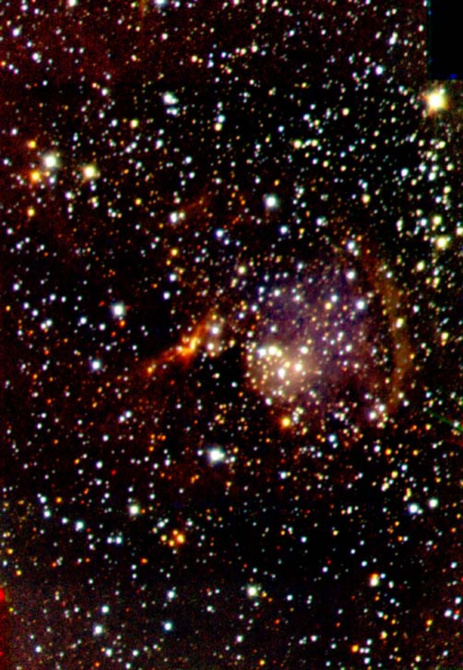
Figure 10: $J$ (blue), $H$ (green) and $K_{S}$ (red) composite colour image of the cluster ionizing the compact H ii region (NTT observations). The field size is $2\hbox{$.\mkern-4.0mu^{\prime}$}66\times 3\hbox{$.\mkern-4.0mu^{\prime}$}85$. North is up, east is left

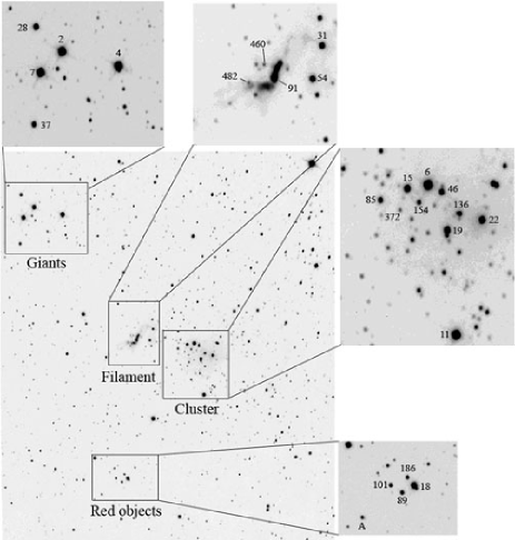
Figure 11: NTT $K_{S}$ image centred on the compact H ii region. The regions and stars discussed in the text are identified

The stellar cluster exciting the compact H ii region As shown in Fig. 11, stars 6, 15, 19, 22, 46, 85, 136, 154 and 372 are observed in the direction of the central cluster. The nature and visual extinction of those sources, derived from the magnitude-colour and colour-colour diagrams, are given in Table 3. Stars 6, 15, 19, 22, 46, 85 and 136 are probably main-sequence stars affected by a visual extinction in the range 3 – 22 mag, possibly indicating large small-scale variations of the visual extinction. Note that massive stars have no pre-main sequence phase and are already on the main-sequence while still accreting matter. Inside the cluster, stars 6 and 22 are bright at all wavelengths. Star 6 is the dominant exciting star of the compact H ii region. According to the absolute calibration of Martins et al. (mar05 (2005)) its $K$ magnitude points to a spectral type between O6 and O7 (Fig. 7), hence earlier than what is derived from the radio observations (Sect. 2.1). However, part of the stellar radiation may escape and not be used to ionize the gas, leading to an underestimate of the spectral type using radio observations. Near-IR spectroscopy is needed to discuss the spectral type of young massive stars (Repolust et al. rep05 (2005)). Star 22 seems to be associated with diffuse emission on the 4.5 $\mu$m and 8 $\mu$m frames of the GLIMPSE survey. (However the GLIMPSE resolution does not allow determination of the magnitudes of the individual stars in the cluster). Stars 154 and 372 show a near-IR excess. The colour-colour diagram of Fig. 8 shows that star 11 is a giant. This is confirmed by its $[3.6]-[4.5]$ colour, and by its non-detection at 8 $\mu$m.

A faint red arc is observed in the $K_{S}$ frame, north-west of the cluster centre (Fig. 10). This arc outlines the limits of the compact H ii region. The origin of this red emission may be fluorescent H₂ emission from the hot PDR and included in the $K_{S}$ band at 2.12 $\mu$m. H₂ at 2.12 $\mu$m and dust emission are known to coincide spatially in Galactic PDRs due to a common excitation origin from UV photons and to the efficient formation of H₂ molecules on the surface of grains (Habart et al. hab03 (2003), Zavagno & Ducci zav01 (2001)). The complete emission shell that outlines the ionization front is not observed in $K_{S}$ but clearly appears at 8 $\mu$m in the GLIMPSE frame (Fig. 4 bottom). This indicates that the zone surrounding the central cluster is more affected by extinction in the south and east.

The filament A red filament is observed 57^′′ (1.2 pc) north-east of the central cluster (Figs. 10 and 11). The emission peak of this filament corresponds to object 91, which shows a near-IR excess (Fig. 8). Maser sources are observed in the exact direction of object 91 (see Sect. 2). Furthermore the near-IR colours of object 91 are in good agreement with the ones found in high-mass star forming regions, at the positions of maser emissions (Goedhart et al. goe02 (2002)). Object 91 is a bright Class I object (Figs. 4 and 9). All this shows that massive-star formation is presently taking place in this region.

Other objects observed towards this region (31, 54, 482) show a near-IR excess, reinforcing the idea of an active and recent star forming region. Object 54 seems to be associated with a small nebulosity, conspicuous on the 8 $\mu$m GLIMPSE image (Figs. 4 bottom).

The red objects group A group of four very red objects (18, 89, 101, 186) is observed south-east of the central cluster (see Fig. 11). An additional isolated red source (object A) is observed nearby. This zone is located at the south border of condensation 2 (Fig. 4 top). As seen in Fig. 8 object 101 is a reddened giant. Sources 18 and A have a near-IR excess. Source A is the reddest object of the field, with $H-K_{S}=2.59$ (it is not detected in $J$ which indicates that $J\geq$ 19.5 and therefore $J-H\geq$ 2.7). Sources 18 and A brighten at longer wavelengths, as shown by the GLIMPSE data (Fig. 4). Fig. 9 shows that sources A and 18 are Class I objects with rising SEDs.

The nature of objects 89 and 186 is not clear. They are brighter than B2V stars, but they have no associated H ii regions; according to Fig. 8 they do not present a near-IR excess. They are very reddened, thus probably are not foreground objects. Star 89 has the $[3.6]-[4.5]$ colour of a giant, and both sources disappear at longer wavelengths; we propose that both are giants, even if it is not clear from Fig. 8.

Many other red sources are observed in the near IR. Those sources are probably located behind the filamentary dust structures observed in the mid-IR that outline the PDR associated with the compact H ii region (see Fig. 4). These objects are too faint to be detected on the GLIMPSE images and are not, therefore, discussed here.

Reddened giants A group of reddened giants is observed on the upper north-eastern part of the field (Fig. 11). This zone contains very luminous objects (2, 4, 7, 28, 37) as shown by Fig. 7. The colour-colour diagram of Fig. 8 reveals that all those sources are reddened giants affected by a visual extinction in the range 5–27 mag. Those reddened sources are visible in the GLIMPSE images and possess specific colours (Fig. 9) that make them easy to identify as giants (Indebetouw et al. ind05 (2005)).

Object 237 is particularly interesting as a bright Class I source that appears isolated on the GLIMPSE images (Fig. 4). It is a faint $K_{S}$ source with a near-IR excess (Fig. 8) and a strongly rising SED. This source is probably a massive young stellar object.

Condensation 3

As seen in Fig. 5, several luminous red objects are observed in the direction of condensation 3. Objects 1, 3 and 5 (1C3, 3C3 and 5C3, respectively) are Class I sources (Fig. 9). Object 1 is relatively faint in $K_{S}$ and has a near-IR excess (Fig. 8). Object 3 is highly reddened and is probably a high mass object. Object 5 has a near-IR excess (Fig. 8) confirming its nature as a young star. Object 2 has GLIMPSE colours very similar to those of the filaments. It may be a B star surrounded by a small PDR. From Fig. 9 the nature of object 4 is not clear, possibly due to the proximity of another star. However, the near-IR data indicate that this source may be a giant (Figs. 8, 7).

Condensation 4

As seen in Fig. 6, several luminous red objects lie along the border of condensation 4, close to the ionized gas, but none are observed at the condensation’s millimetre emission peak. These objects are of different nature. Object 1 (1C4) is a small nebulosity of about 0.3 pc $\times$ 0.4 pc around a central star. Its GLIMPSE colours are very similar to those of the filaments. This extended emission probably originates from a PDR region associated with star 1, a B star with a visual extinction of 7 mag. The near-IR data indicate a massive main-sequence source. Object 2 (2C4) is also a small nebulosity with the colours of the filaments. This source is relatively faint in the $K_{S}$ band and may have a near-IR excess if it is a low mass object. Objects 3 (3C3)and 4 (4C4) are Class I objects (Fig. 9). Object 4 is particularly interesting as it is a high luminosity source, one of the brightest objects seen by GLIMPSE in the RCW 79 field, apart from giants. This object has a large near-IR excess ((Fig. 8) and is probably a young massive star. Object 5 (5C4) is a red giant with a visual extinction of 20 mag. This is confirmed by its position in Figs. 7, 8 and 9, lying in the giant region where numerous stars are observed. Object 6 (6C4) is situated at the head of a bright rim surrounding condensation 6 (Fig. 6). It is a Class I or Class II object (Fig. 9). This source is bright in $K_{S}$ (Fig. 7) and has a near-IR excess (Fig. 8).

No stars are observed at the millimetre peak of the condensations. This indicates either that no stars are there at all, or that earlier phases of star formation have taken place but are not detected in the mid IR due to the low temperature of the sources and the high extinction. Typical spectral energy distribution of Class 0 sources shows mid-IR fluxes below the GLIMPSE detection limits. Deeper mid-IR observations are needed to address the question of star formation at condensations millimetre peak.

Fig. 9 shows that twelve Class I sources, associated with the three most massive millimetre condensations, are observed at the periphery of RCW 79. Some of those sources are very bright and have near-IR excess and are thus possibly massive young stellar objects. This result indicates that we are observing a case of relatively recent massive-star formation at the borders of RCW 79.

4.3 The velocity field of the ionized gas

Figure 12 presents the H$\alpha$ velocity field of RCW 79. The zones of brightest H$\alpha$ emission have a mean velocity of $-$44 km s^-1. An annular structure of more diffuse emission, with a velocity $\sim$ $-$50 km s^-1, limits the H ii region; especially, at the southern border of RCW 79, a clear arc-like structure is observed at $-$51 km s^-1. The H$\alpha$ emission observed at 13^h40^m10$.\!\!^{\rm s}$3, $-$61^∘38^′35^′′, in the direction of the “hole” observed in the dust ring, has a velocity of $-$40 km s^-1. Thus, the shape of the dust ring surrounding the ionized region, with its conspicuous hole, and the velocity field showing a flow of ionized material at a few km s^-1, suggest that the molecular environment of RCW 79 is broken in the north-west, and that the ionized gas is flowing away from the centre of the H ii region through this hole. This is coherent with the observed location of the most massive condensations to the south and west, limiting the ionized zone more efficiently in this direction. The presence of a molecular cloud to the south of RCW 79 (Saito et al. sai01 (2001)) corroborates this interpretation.

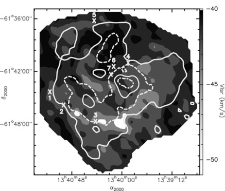
Figure 12: Grey-scale image of the H$\alpha$ velocity field of RCW 79. The map is overlaid with H$\alpha$ intensity contours (in arbitrary units). The peak positions of the 1.2-mm condensations are indicated (white cross)

The observed $-$51 km s^-1 to $-$40 km s^-1 H$\alpha$ velocity range is in good agreement with the velocities measured from the H109$\alpha$ radio recombination line by Wilson et al. (wil70 (1970), $-$46.4 and $-$51.8 km s^-1, 4^′ HPBW). Similar velocities are measured for the associated molecular gas, from the CS (2 – 1) emission line by Bronfman et al. (bro96 (1996), $-$48 km s^-1, 50^′′ HPBW), and for the methanol maser observed in the direction of IRAS 13374$-$6130 by Caswell (cas04 (2004), $-$51 km s^-1).

CGPMC report a lack of H i emission, obtained from the Southern Galactic Plane Survey (SGPS, McClure-Griffiths et al. mcc05 (2005)) observed between $-$26.4 and $-$28.9 km s^-1 (see their fig. 13). The shape of this absorption strongly suggests that it is associated with the H ii region RCW 79. We checked the H i data cube and observed an H i absorption at $-$25.6 km s^-1 that has the same structures as the ones seen in the H$\alpha$ emission, especially the northern H$\alpha$ flow. However the H i velocity does not correspond to that observed for the ionized gas. A problem of H i velocity calibration may occur in this case.

5 Comparison with the model of Whitworth et al.

Whitworth et al. (whi94 (1994)) have developed an analytical model to describe the fragmentation of the shocked dense layer surrounding an expanding H ii region. In particular, these authors predict the time at which the fragmentation occurs, the size of the H ii region at that moment, the column density of the layer, the masses of the fragments and their separations along the layer. The adjustable parameters of the model are $\dot{\cal N}_{\rm{\tiny{Lyc}}}$, the number of Lyman continuum photons emitted per second by the exciting star, the density $n_{\tiny{{0}}}$ of the surrounding homogeneous infinite medium into which the H ii region expands, and $a_{\rm{\tiny{S}}}$, the isothermal sound speed in the compressed layer. The derived quantities depend weakly on $\dot{\cal N}_{\rm{\tiny{Lyc}}}$, somewhat on $n_{\tiny{{0}}}$, and strongly on $a_{\rm{\tiny{S}}}$.

Whitworth et al. point out that the adopted value of 0.2 km s^-1 for $a_{\rm{\tiny{S}}}$ is likely to represent a lower limit of the sound speed in the layer, as both turbulence generated by dynamical instabilities and extra heating from intense sub-Lyman-continuum photons leaking from the H ii region tend to increase this value. This point is very important because the mass of the fragments depends strongly on this velocity: $M_{\rm{fragment}}\propto a_{\rm{\tiny{S}}}^{40/11}$. Estimating an accurate value of $a_{\rm{\tiny{S}}}$ in the hot PDR surrounding an H ii region is an important issue, especially for a realistic comparison with analytical models. In the following we will consider values in the range 0.2–0.6 km s^-1.

RCW 79 appears as an “isolated” H ii region, as observed in large scale mid-IR images (MSX and Spitzer). The ¹³CO integrated intensity map indicates that dense material, with densities of $10^{3}$ cm^-3, is present in condensations at the periphery of the ionized region, with weak emission outside this structure (see Saito et al. sai01 (2001)). In the following we will consider densities in the range 300–3000 cm^-3.

The rate of Lyman continuum photon emission by the exciting star of RCW 79 is 2.9 $\times\leavevmode\nobreak\ 10^{49}$ photons s^-1 (Sect. 2). We adopt this value in the following.

According to Whitworth et al., the time at which the fragmentation starts is

$$t_{\mathrm{frag}}\approx 1.42\,\,a_{\rm{.2}}^{7/11}\,\,n_{3}^{-5/11}\,\mathrm{Myr}\,,$$

the radius of the ionized region is then

$$R_{\mathrm{frag}}\approx 6.4\,\,a_{\rm{.2}}^{4/11}\,\,n_{3}^{-6/11}\,\mathrm{pc}\,,$$

and the mass of the fragments is

$$M_{\mathrm{frag}}\approx 20.9\,a_{.2}^{40/11}\,\,n_{3}^{-5/11}\,M_{\odot}\,,$$

where $a_{\rm{.2}}=a_{\rm s}/0.2$ and $n_{3}=n_{\tiny 0}/1000$ are dimensionless variables.

The actual radius of the H ii region, $R\sim$ 6.4 pc, allows us to estimate its dynamical age, $t_{\mathrm{dyn}}$, which depends of the density of the medium into which the region evolves. According to Osterbrock (ost89 (1989)), a star emitting 2.9 $\times\leavevmode\nobreak\ 10^{49}$ ionizing photons per second forms a Strömgren sphere of radius $R_{0}\,\,(\mathrm{pc})\leavevmode\nobreak\ =\leavevmode\nobreak\ 0.965\,\,n_{3}^{-2/3}$. This ionized region expands; according to Dyson & Williams (dys97 (1997)), its radius varies with time as

$$R=R_{0}(1+2.15\times 10^{-5}\leavevmode\nobreak\ t_{\mathrm{dyn}}/R_{0})^{\frac{4}{7}},$$

where $R$ and $R_{0}$ are in parsecs and $t_{\mathrm{dyn}}$ in years.

Fig. 13 shows how $t_{\mathrm{dyn}}$ and $t_{\mathrm{frag}}$ vary as a function of $n_{\tiny{{0}}}$, for three values of $a_{\rm{\tiny{S}}}$ (0.2, 0.4, and 0.6 km s^-1). Of course, $t_{\mathrm{dyn}}$ must be larger than $t_{\mathrm{frag}}$, as we are seeing molecular fragments already formed at the border of RCW 79. This indicates that $n_{\tiny{{0}}}\geq 1200$ cm^-3 if $a_{\rm{\tiny{S}}}$= 0.2 km s^-1, or $n_{\tiny{{0}}}\geq 2400$ cm^-3 if $a_{\rm{\tiny{S}}}$= 0.6 km s^-1.

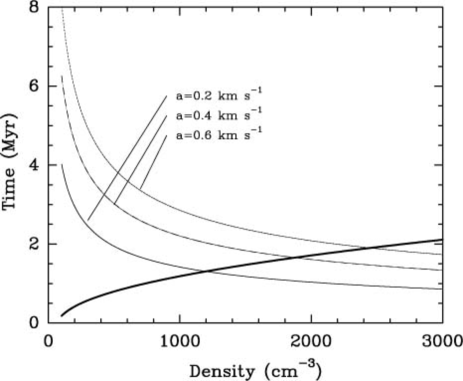
Figure 13: Variations of $t_{\mathrm{dyn}}$ (thick curve) and $t_{\mathrm{frag}}$ (thin curves) as a function of the density, $n_{\tiny{{0}}}$, for the observed radius of 6.4 pc and three values of $a_{\rm{\tiny{S}}}$ (0.2, 0.4, and 0.6 km s^-1), respectively

In the same way Fig. 14 shows the radius of the layer at the time of fragmentation, $r_{\mathrm{frag}}$, as a function of $n_{\tiny{{0}}}$. This can be compared with the actual radius of the H ii region, which must be larger than $r_{\mathrm{frag}}$ as fragmentation has occured. This shows that $n_{\tiny{{0}}}\geq 950$ cm^-3 if $a_{\rm{\tiny{S}}}$= 0.2 km s^-1, or $n_{\tiny{{0}}}\geq 2000$ cm^-3 if $a_{\rm{\tiny{S}}}$= 0.6 km s^-1.

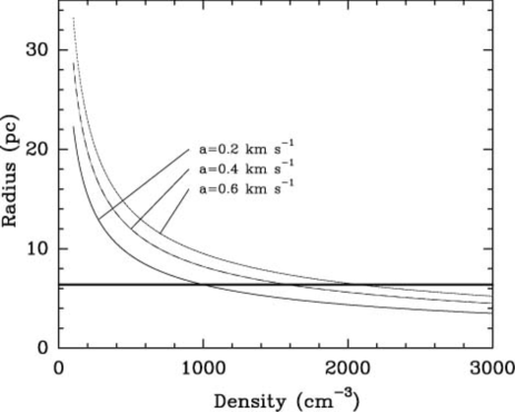
Figure 14: Radius of the layer at the time of fragmentation (thin curves), $r_{\mathrm{frag}}$, as a function of the density, $n_{\tiny{{0}}}$. The actual radius of RCW 79, 6.4 pc is shown (thick line)

Fig. 15 allows one to compare the mass of the fragments estimated by the model and the mass of the most massive observed condensation. This comparison shows that massive fragments can only form if $a_{\rm{\tiny{S}}}$ is high.

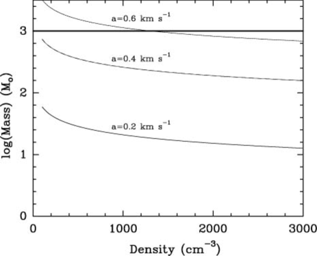
Figure 15: Mass of the fragments (thin curves) predicted by the model compared with the mass of the most massive observed condensation, as a function of density, $n_{\tiny{{0}}}$. The mean mass of the most massive fragment ($\simeq$1000 $M_{\hbox{$\odot$}}$) is shown (thick line)

Adopting a reasonable value of $n_{\tiny{{0}}}=2000$ cm^-3, we estimate a dynamical age of 1.7 Myr for RCW 79. According to the model and assuming $a_{\rm{\tiny{S}}}=0.4$ km s^-1, fragmentation occured some 10⁵ years ago, after 1.6 Myr of evolution; the radius of the H ii region was then 5.6 pc. This constrains the age of the compact H ii region and its exciting cluster. We adopt, for the radius of this region, 1.7 pc, which is the radius of the 8 $\mu$m PAHs emission ring surrounding it. A dynamical age of 0.13 Myr is then estimated for the compact H ii region, assuming $n_{\tiny{{0}}}\leavevmode\nobreak\ =\leavevmode\nobreak\ 3000$ cm^-3 for $a_{\rm{\tiny{S}}}=0.4$ km s^-1. This result is compatible with the general evolutionary scheme of RCW 79, in particular with the high number of Class I sources (of age of about 10⁵ years) observed towards the most massive fragments. However the model does not account for the large masses of fragments 2, 3 and 4 ($M_{\mathrm{frag}}\sim 200\leavevmode\nobreak\ M_{\hbox{$\odot$}}$ with the adopted figures; see Fig. 15). Note that adopting a higher value for the sound speed (0.6 km s^-1) and a higher density (2500 cm^-3) lead to an unreasonably young dynamical age of 37000 years for the compact H ii region.

The model of Whitworth et al. assumes expansion into an infinite and homogeneous medium. This is probably unrealistic and may explain some of the discrepancies between the predictions of the model and the observations. A massive star forms in a dense core, but as the H ii region grows in size it probably expands into a medium of lower density. Hence the necessity of models taking into account evolution in a non-homogeneous medium, such as the models developed by Hosokawa (private communication). Also, Whitworth et al. assume spherical symmetry around the exciting star. Thus some fragments, and subsequently some YSOs, should be observed in the direction of the ionized gas. This is not the case: in RCW 79, as well as in Sh 104 (Deharveng et al. deh03 (2003)), the main fragments and the YSOs seem to form in a preferential plane. Thus non spherical models are also needed.

Other star-formation triggering mechanisms such as the pressure-induced collapse of pre-existing clumps (Lefloch & Lazareff lef94 (1994)) and/or the growth of dynamical instabilities in the collected layer (Garcia-Segura & Franco gar96 (1996)) cannot be ruled out in the case of RCW 79. In particular, the morphology of the south-west ionization front, as traced by the GLIMPSE 8 $\mu$m filaments, is very chaotic, showing protruding structures (elephant trunks or small-scale bright rims). The presence of such small-scale structures is expected if the ionization front moves into an inhomogeneous medium, or if small-scale clumps are formed on short time scales by dynamical instabilities. For example, the formation of object 6 near condensation 4 (Fig. 6), observed on the top of a bright rim, probably results from the pressure induced-collapse of such a structure. However, the more massive fragments observed along the annular collected layer, and especially the most massive fragments (condensations 2 and 4), diametrically opposite each other along this ring, point to a prevailing large-scale, long time scale mechanism such as the collect and collapse process.

6 Conclusions

We have presented a new 1.2-mm continuum map and near-IR images of the Galactic H ii region RCW 79. The 1.2-mm map reveals the presence of a layer of cold dust at the periphery of the ionized region. This material has most probably been collected, during the expansion of the H ii region, between the ionization and the shock fronts. This layer is presently fragmented. Five large and massive fragments are observed along the borders of RCW 79. The two most massive fragments are diametrically opposite in this layer.

The three most massive fragments are associated with young, massive objects, as revealed by near- and mid-IR data. These objects are mainly luminous Class I sources. Some other are associated with nebulosities with typical mid-IR colours of filaments in PDRs, indicating that they are possibly early B stars surrounded by small PDRs.

Signposts of recent star formation (maser emission associated with a Class I source) nearby a compact H ii region indicate that star formation is still active there.

Kinematic information from H$\alpha$ observations reveals that RCW 79 may experience a champagne phase acting as a destructor of the surrounding annular structure. This fact complicates the modeling of this region . However, it is probable that the fragmentation of the annular structure occurred prior to the champagne phase. The formation of massive fragments in the layer favours the creation of lower density zones through which the ionized gas can escape easily.

The analytical model of Whitworth et al. whi94 (1994), describing the collect and collapse process, accounts for the global properties of this region. RCW 79 is 1.7 Myr old; the collected layer fragmented some 10⁵ yrs ago; this is also the age of the compact H ii region observed at the periphery of RCW 79, of its exciting cluster and also probably of the numerous Class I sources observed towards the most massive fragments. The large masses of the observed fragments indicate a large sound velocity (at least 0.4 km s^-1) in the compressed layer; this is to be expected in a hot PDR surrounding an H ii region. However the observations show that the fragments and the massive YSOs are all found in a preferential plane, which cannot be explained by Whitworth’s model. Non-spherical, non-homogeneous density models are needed.

Different processes of triggered star formation are probably simultaneously at work in this region. Some YSOs are associated with small-scale structures such as bright rims. Their formation has probably been triggered by the pressure-induced collapse of a pre-existing molecular clumps, or of clumps resulting from dynamical instabilities in the collected layer. The large and massive fragments observed at the periphery of RCW 79 most probably result from the gravitational collapse of the layer of collected material, according to the collect and collapse process.

All the new observational facts presented in this paper indicate that we are dealing with the collect and collapse process as the main triggering agent of massive star formation at the borders of RCW 79. The presence of obscured zones towards the peaks of the millimetre condensations indicate that precursor sites of massive-star formation may still be present, representing ideal sites to address the question of massive star formation.

- (1) Allen, L.E., Calvet, N., D’Alessio, P., Merin, B., Hartmann, L., Megeath, S.T., Gutermuth, R.A., Muzerolle, J. Pipher, J.L., Myers, P.C., Fazio, G.G., 2004, ApJS, 154, 363
- (2) Benjamin, R.A., Churchwell, E., Babler, B.L., Bania, T.M., Clemens, D.P., Cohen, M., Dickey, J.M., Indebetouw, R., Jackson, J.M., Kobulnicky, H.A. et al. 2003, PASP, 115, 953
- (3) Bonnarel, F., Fernique, P., Bienayme, O., Egret, D., Genova, F., Louys, M., Ochsenbein, F.,Wenger, M., Bartlett, J.G. 2000, A&ASS, 143, 33
- (4) Bronfman, L., Nyman, L.-A., May, J. 1996, A&AS, 115, 81
- (5) Caswell, J.L., Haynes, R.F., 1987, A&A, 171, 261
- (6) Caswell, J.L. 2004, MNRAS, 351, 279
- (7) Chini, R., Kämpgen K., Reipurth, B., Albrecht, M., Kreysa, E., Lemke, R., Nielbock, M., Reichertz, L.A., Sievers, A., Zylka, R. 2003, A&A, 409, 235
- (8) Condon, J. J., Cotton, W. D., Greisen, E. W., Yin, Q. F., Perley, R. A., Taylor, G. B., Broderick, J. J. 1998, AJ, 115, 1693
- (9) Cohen, M., Green, A. J., Parker, Q.A., Mader, S., Cannon, R. D. 2002, MNRAS, 336, 736
- (10) Deharveng, L., Lefloch, B., Zavagno, A., Caplan, J., Whitworth, A.P., Nadeau, D., Martin, S., 2003, A&A, 408, L25
- (11) Deharveng, L., Zavagno, A., Caplan, J. 2005, A&A, 433, 565: paper I
- (12) Dyson, J.E., Williams, D.A. 1997, The physics of the interstellar medium, 2nd ed., eds R J Tayler & M Elvis, Published by Institute of Physics Publishing, Bristol and Philadelphia
- (13) Elmegreen, B. G., Lada, C.J. 1977, ApJ, 214, 725
- (14) Elmegreen, B. G. 1998, in ASP Conf. Ser., 148, 150 ed. C. E. Woodward, J. M. Shull & H. A. Tronson
- (15) Egan, M. P., Price, S. D., Moshir, M. M., et al. 1999, The Midcourse Space Experiment Point Source Catalog Version 1.2, Explanatory Guide, AFRL-VS-TR-1999-1522, Air Force Research Laboratory
- (16) Fazio, G.G., Hora, J.L., Allen, L.E., Ashby, M.L.N., Barmby, P., Deutsch, L.K., Huang, J.-S., Kleiner, S., Marengo, M., Megeath, S.T. et al. 2004, ApJS, 154, 10
- (17) García-Segura, G., Franco, J. 1996, ApJ, 469, 171
- (18) Goedhart, S., van der Walt, D. J., Gaylard, M. J. 2002, MNRAS, 335, 125
- (19) Green, A.J. 1999, ASP Conf. Ser., 168, 43
- (20) Habart, E., Boulanger, F., Verstraete, L., Pineau des Forêts, G., Falgarone, E., Abergel, A. 2003, A&A, 397, 623
- (21) Hildebrand, R.H. 1983 Q.Jl. R. astr. Soc., 24, 267
- (22) Indebetouw, R., Mathis, J. S., Babler, B. L., Meade, M. R., Watson, C., Whitney, B. A., Wolff, M. J., Wolfire, M. G., Cohen, M., Bania, T. M. et al. 2005, ApJ, 619, 931
- (23) Koornneef, J. 1983 A&A, 128, 84
- (24) Le Coarer, E., Amram, P., Boulesteix, J., Georgelin, Y. M., Georgelin, Y. P., Marcelin, M., Joulie, P., Urios, J. 1992, A&A, 257, 389
- (25) Lefloch, B., Lazareff, B., 1994 A&A, 289, 559
- (26) Léger, A., Puget, J.-L. 1984, A&A, 137, L5
- (27) Mathis, J.S. 1990, ARA&A, 28, 37
- (28) Martins, F., Schaerer, D., Hillier, D.J. 2005, submitted to A&A (astro-ph/0503346)
- (29) McClure-Griffiths, N.M., Dickey, J.M., Gaensler, B.M., Green, A.J., Haverkorn, M., Strasser, S. 2005, ApJS, 158, 178
- (30) Megeath, S.T., Gutermuth, R.A., Allen, L.E., Pipher, J.L., Myers, P.C., Fazio, G.G. 2004, ApJS, 154, 367
- (31) Morisset, C., Schaerer, D., Bouret, J.-C., Martins, F. 2004, A&A, 415, 577
- (32) Motte, F., Schilke, P., Lis, D.C. 2003, ApJ, 582, 277
- (33) Ossenkopf, V., Henning, T. 1994 A&A, 291, 943
- (34) Osterbrock, D.E. 1989, Astrophysics of Gaseous Nebulae and Active Galactic Nuclei, University Science Books, Mill Valley, California
- (35) Parker, Q.A., Phillipps, S., 1998, PASA, 15, 28
- (36) Persson, S.E., Murphy, D.C., Krzeminski, W., Roth, M., Rieke, M.J. 1998, AJ, 116, 2475
- (37) Price, S.D., Egan, S.M., Carey, S.J., Mizuno, D.R., Kuchar, T.A. 2001, AJ, 121, 2819
- (38) Repolust, R., Puls, J., Hanson, M.M., Kudritzki, R.-P., Mokiem, M.M. 2005, A&A in press (astro-ph/0501606)
- (39) Rodgers, A. W., Campbell, C. T., Whiteoak, J. B. 1960, MNRAS, 121, 103
- (40) Russeil, D. 2003, A&A, 397, 133
- (41) Saito, H., Mizuno, N., Morigichi, Y., Matsunaga, K., Onishi, T., Mizuno, A., Fukui, Y. 2001, PASJ, 53, 1037
- (42) Schaerer, D., de Koter, A. 1997, A&A, 322
- (43) Schmidt-Kaler, T. 1982, In: Schaifers, K., Voigt, H.H. (eds) Landolt-Bornstein, New Series, Group IV, Vol. 2, Springer-Verlag, Berlin, p. 1
- (44) Simpson, J.P., Rubin, R.H. 1990, ApJ, 354, 165
- (45) Smith, L., Norris, R.P.F., Crowther, P.A. 2002, MNRAS, 337, 1309
- (46) Stetson, P.B. 1987, PASP, 99, 191
- (47) Vacca, W.D., Garmany, C.D., Shull, J.M. 1996, ApJ, 460, 914
- (48) van der Walt, D.J., Gaylard, M.J., MacLeod, G.C. 1995, A&AS, 110, 81
- (49) Wilson, T.L., Mezger, P.G., Gardner, F.F., Milne, D.K. 1970, A&A, 6, 364
- (50) Whitney, B.A., Indebetouw R., Bjorkman, J.E., Wood, K. 2004, ApJ, 617, 1177
- (51) Whitworth, A.P., Bhattal, A.S., Chapman, S.J., Disney, M. J., Turner, J.A. 1994, MNRAS, 268, 291
- (52) Wright, A.E., Griffith, M.R., Burke, B.F., Ekers, R. D. 1994, ApJS, 91, 111
- (53) Zavagno, A., Ducci, V. 2001, A&A, 371, 312