Gamma-ray continuum emission from the inner Galactic region as observed with INTEGRAL/SPI

The diffuse continuum emission from the Galactic plane in the energy range 18-1000 keV has been studied using 16 Ms of data from the SPI instrument on INTEGRAL. With such an exposure we can exploit the imaging properties of SPI to achieve a good separation of point sources from the various diffuse components. Using a candidate-source catalogue derived with IBIS on INTEGRAL and a number of sky distribution models we obtained spectra resolved in Galactic longitude. We can identify spectral components of a diffuse continuum of power law shape with index about 1.7, a positron annihilation component with a continuum from positronium and the line at 511 keV, and a second, roughly power-law component from detected point sources. Our analysis confirms the concentration of positron annihilation emission in the inner region ($|l|<10^{o}$), the disk ($10^{o}<|l|<30^{o}$) being at least a factor 7 weaker in this emission. The power-law component in contrast drops by only a factor 2, showing a quite different longitude distribution and spatial origin. Detectable sources constitute about 90% of the total Galactic emission between 20 and 60 keV, but have a steeper spectrum than the diffuse emission, their contribution to the total emission dropping rapidly to a small fraction at higher energies. The spectrum of diffuse emission is compatible with RXTE and COMPTEL at lower and higher energies respectively. In the SPI energy range the flux is lower than found by OSSE, probably due to the more complete accounting for sources by SPI. The power-law emission is difficult to explain as of interstellar origin, inverse Compton giving at most 10%, and instead a population of unresolved point sources is proposed as a possible origin, AXPs with their spectra hardening above 100 keV being plausible candidates. We present a broadband spectrum of the Galactic emission from 10 keV to 100 GeV.

1 Introduction

Interstellar gamma-ray emission from the Galaxy is a major study objective for INTEGRAL. The inner Galactic ridge is known to be an intense source of continuum hard X- and soft $\gamma$-ray emission: hard X-ray emission was discovered in 1972 (Bleach et al., 1972), and interstellar emission has subsequently been observed from keV to MeV energies by ASCA, Ginga, RXTE, OSSE, COMPTEL and most recently by Chandra and XMM-Newton. Most directly comparable to our INTEGRAL analysis are results from OSSE on the Compton Gamma Ray Observatory (Purcell et al., 1996; Kinzer et al., 1999, 2001).

Continuum emission of diffuse, interstellar nature is expected in the hard-X and $\gamma$-ray regime from the physical processes of positron annihilation (through intermediate formation of positronium atoms) and of inverse-Compton emission or bremsstrahlung from cosmic-ray electrons. For the non-positronium continuum, hard X-rays from bremsstrahlung emission imply a luminosity in cosmic-ray electrons which is unacceptably large (see e.g. Dogiel et al., 2002a). Composite models have been proposed, with thermal and nonthermal components from electrons accelerated in supernovae or ambient interstellar turbulence, by Valinia et al. (2000b). An alternative solution to the luminosity problem has been proposed by Dogiel et al. (2002b). At MeV energies the origin of the emission is also uncertain (Strong et al., 2000).

Alternatively, the origin of the ridge emission could be attributed to a population of sources too weak to be detected individually, and hence it could be not truly interstellar. Gamma-ray telescopes in general have inadequate spatial resolution to clarify this issue. For X-rays, important progress in this area was made by ASCA (Kaneda et al., 1997) and Ginga (Yamasaki et al., 1997). More recently, high-resolution imaging in X-rays (2–10 keV) with Chandra (Ebisawa et al., 2001, 2005) has proven the existence of a truly diffuse component; similarly, it has been inferred from XMM-Newton (Hands et al., 2004) that 80% of the Galactic-ridge X-ray emission is probably diffuse, and only 9% can be accounted for by Galactic sources (the rest being extragalactic sources).

The study of the Galactic-ridge continuum emission is a key goal of the INTEGRAL mission. The high spectral resolution combined with its imaging capabilities promises new insights into the nature of this enigmatic radiation. Furthermore, reliable modelling of the diffuse emission will be essential for the study of point sources in the inner Galaxy, since it constitutes a large and anisotropic background against which sources must be resolved.

Previous work based on first, smaller sets of INTEGRAL/SPI observations have reported the detection of diffuse emission at a level consistent with previous experiments (Strong et al., 2003; Strong, 2003). But statistical and systematic errors were large, due in part to the uncertainty in the point-source contribution. Meanwhile, a new analysis of INTEGRAL/IBIS data (Lebrun et al., 2004; Terrier et al., 2004) showed that, up to 100 keV, indeed a large fraction of the total emission from the inner Galaxy is due to sources. Strong et al. (2004c) used the source catalogue from this work (containing 91 sources) as input to SPI model fitting, giving a much more solid basis for the contribution of point sources in such an analysis. This exploited the complementarity of the instruments on INTEGRAL for the first time in the context of diffuse emission. In the present work we extend this analysis to include a much larger observation database, and use the 2nd IBIS Catalogue to provide source candidates.

We also draw attention to a related paper (Bouchet et al., 2005), which describes an independent but similar study of SPI data, but focussing more on the point-source contribution.

2 INTEGRAL Observations

The INTEGRAL Core Program (Winkler et al., 2003) for A01 includes the Galactic Centre Deep Exposure (GCDE) which maps the inner Galaxy ($330^{\circ}<l<30^{\circ},-20^{\circ}<b<20^{\circ}$) with a viewing time of about 4Ms per year. The full region is covered in one GCDE cycle, and there are two cycles per year. Subsequent AOs have varied this strategy somewhat. In addition the Galactic Plane Survey (GPS) covers the whole plane at low Galactic latitude, with lower exposure than the GCDE. Data from the first three years, including GCDE, GPS, data which has become public up to March 2005, and Open Time data for which permission has been obtained from the corresponding Principal Investigator, are used for the study reported here.

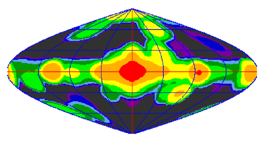
We use data from the SPI (INTEGRAL Spectrometer) instrument; descriptions of the instrument and performance are given in Vedrenne et al. (2003); Attié et al. (2003). The energy range covered by SPI is 20 keV – 8 MeV, but here we restrict the analysis to energies up to 1 MeV; above these energies the statistics are small and the analysis is more difficult, so is reserved for future work. The data were pre-processed using the INTEGRAL Science Data Centre (ISDC) Standard Analysis software (OSA) up to the level containing binned events, with 0.5 keV bins, with pointing and livetime information. GCDE data from about 200 orbital revolutions from 15 – 259 were used. 8100 pointings were used; the sky exposure is shown in Fig 1; the total exposure livetime is $1.6\times 10^{7}$ s. The exposure per pointing is typically 1800 s. The energy calibration is performed using instrumental background lines with known energies; while this is a critical operation for line studies (where sub-keV accuracy is required), for continuum studies a standard calibration ($\sim$1 keV accuracy) is quite adequate. Various energy binnings were used, depending on the available statistics as a function of energy. Only single-detector events are used here, since they dominate below 1 MeV. After the failure of detector 2 at IJD 1434 the remaining 18 detectors were used, and after the failure of detector 17 at IJD 1659 the remaining 17 were used.

The instrumental response is based on extensive Monte Carlo simulations and parameterization (Sturner et al., 2003); this has been tested on the Crab in-flight calibration observations and shown to be reliable to better than 20% in absolute flux at the current state of the analysis.

Since INTEGRAL data are dominated by instrumental background, the analysis needs to have good background treatment methods. In the present work the background ratios between detectors are obtained by averaging the entire dataset over time; this has been found to give results which hardly differ from taking ‘OFF’ observations, and has the advantage of much higher statistics. A check on the systematics in this background approach was given in Strong et al. (2003).

3 Overview of Methods

3.1 Data combination, energy binning, selection

The program spiselectscw combines the observation-by-observation standard-processed data into a single set of datasets suitable for input to analysis software. Its functions include rebinning in energy, rejection of anomalous data (e.g. high rates due to solar flares), and detector selection (singles, multiples). This step is required to reduce the enormous data volume of the standard-processed data (with its 0.5 keV binning) into a manageable form.

3.2 Background template generation

The program spioffback generates a background template by averaging the detector ratios over all pointings (either from a set of high-latitude ‘OFF’ observations or from the ON observations themselves), and using these ratios to compute predicted counts using the livetime information. The total predicted counts are normalized to the total observed counts in each energy interval: this normalization is for convenience, but is not essential since the absolute background level is determined later in the fitting procedure. The template is generated separately for each of the periods separated by detector 2 and 17 failures, since these failures have a signficant impact on the detector ratios.

3.3 Model fitting

The program spimodfit uses the binned count data, pointing and exposure information, and the instrumental response, to fit sky models, point sources and background. The output is in the form of FITS files containing, for all processed energies: the fit parameters, the covariance matrices and the input models. spimodfit is a development (by H. Halloin, MPE) from spidiffit which was used in earlier work (Strong et al., 2003, 2004c). It includes more flexible background fitting, optimized fitting routines and memory use, and improvement formatting of the output. We use spimodfit version 2.4 in this work.

The model skymaps to be fitted are generated with the program gensky, which includes HI and CO survey data, as well as Gaussians of arbitrary position and width. The input source catalogue is in the ISDC catalogue format.

3.4 Spectra

The appropriate size of the energy bins is a trade-off between the high instrumental resolution and the available statistics. Since this cannot be predicted a priori, we make the fits in a range of binsizes over the whole spectrum, and choose for presentation those for which a satisfactory signal-to-noise is achieved. Hence the binsize increases from $\sim$10 keV at low energies to $\sim$100 keV at high energies.

The spectral fitting is done using the full energy redistribution matrix in the form of ‘RMF’ and ‘IRF’ SPI response files (see Section 2 for references). The procedure used is rigorous for the case where the ratio between the three components of the IRF (photopeak and the two Compton components) is independent of incidence direction: this variation is small so the procedure is accurate. The energy response has a significant effect on the fits as can be seen from the difference between the raw data points and the fitted spectra (Figs 4–6). The effect is mainly on the level of the power-law component; for the positronium the effect is small.

3.5 Evaluation and plotting

The program galplot combines the results from many spimodfit runs into spectra integrated over sky regions, and sources. It evaluates the fluxes and error bars using the fit parameters covariance matrices. It plots the SPI spectra together with results from other instruments like RXTE, COMPTEL, EGRET, and theoretical models from the galprop project Strong et al. (2004a, b, d).

4 Model Fitting

4.1 Basic approach

We distinguish image space and data space in the usual way, and define the instrument response as the relation between them. The image is $I_{j}$ and the expected data is $d_{k}$. The expected background is $b_{k}$ Let $R_{jk}$ be the response of data element $k$ to image element $j$. Then

$$d_{k}=\sum_{j}R_{jk}I_{j}+b_{k}$$

For the the special case of an image component consisting of a point source, only the position is required and computing $d_{k}$ requires no convolution.

An image model is a parameterized algorithm for composing an image from components. For a linear model,

$$I_{j}=\sum_{i}\theta_{i}M_{ij}$$

where $\theta_{i}$ are the model parameters.

More generally, the image will still be described by a sum of components, but the image components will be non-linear functions of the parameters (e.g. Gaussian, exponential) and each component is described by several parameters $\overline{\theta}_{i}$:

$$I_{j}=\sum_{i}M_{ij}(\overline{\theta}_{i})$$

Similarly the background can be constructed from components of a background model $B_{ik}$

$$b_{k}=\sum_{i}\theta_{i}B_{ik}$$

where $\theta_{i}$ now introduces background parameters. The sums in the above expressions are over the appropriate subsets of parameters for image and background model respectively. In this way we can treat image and background model in the same way in the subsequent analysis, and $\theta_{i}$ includes both. The only formal difference between image and background model is that the image is convolved with $R_{jk}$ and the background is not:

$$d_{k}=\sum_{j}R_{jk}\sum_{i=1}^{i=N_{I}}\theta_{i}M_{ij}+\sum_{i=N_{I}+1}^{i=N_{I}+N_{B}}\theta_{i}B_{ik}$$

where there are $N_{I}$ image components and $N_{B}$ background components, and $N=N_{I}+N_{B}$.

In our modelling approach, the measured signal is represented through model components:

$$d_{k}=\sum_{i}\theta_{i}S_{ik}$$

where the sky part (diffuse + sources) is:

$$S_{ik}=\sum_{j}R_{jk}M_{ij},\ \ \ \ i=1,N_{I}$$

and the instrumental-background part is:

$$S_{ik}=B_{ik},\ \ \ \ i=N_{I}+1,N_{I}+N_{B}$$

Details of the statistical model fitting method are given in Appendix A.

5 The models

5.1 Diffuse Galactic emission

Model maps to represent the emission from cosmic-ray interactions with the gas are integrated HI and ¹²CO as described in Strong et al. (2004a). Other components, including positronium, positron line, bulge and Galactic plane, are represented by a set of Gaussians of various widths summarized in Table 1. For the positronium and positron line we include Gaussians with FHWM = 5^∘, 10^∘ (Jean et al., 2003; Knödlseder et al., 2003). Generally only the sum of the components are presented since the separate components do not necessarily have physical significance; the idea is to include sufficient aspects of Galactic structure to be able to reproduce the total emission with reasonable confidence. Summing subsets of components allows a morphological decomposition of the spectrum for example into disc and bulge emission.

Note that our model components are not orthogonal, but this is not a problem since our use of the covariance matrix explicitly handles the parameter correlations and the computation of the errors on linear combinations of components.

Table 1: Diffuse model components used in the fitting

Component	description	longitude	latitude
		FWHM (deg)	FWHM (deg)
1	HI
2	CO
3	Gaussian	40	5
4	Gaussian	60	5
5	Gaussian	80	5
6	Gaussian	5	5
7	Gaussian	10	5
8	Gaussian	20	5
9	Gaussian	10	10

5.2 Sources

The sources fitted are based on a preliminary version of the 2nd ISGRI Catalogue (Bird et al., 2005), containing 209 sources. Only the source coordinates are used here, since the flux in each energy range is determined in the fitting procedure simultaneously with the other components.

At low energies it is known that most of the catalogue sources are detectable and make a corresponding contribution to the emission. At high energies on the other hand, only a few sources have a hard enough spectrum to be of relevance. Including the whole catalogue in fact leads to a ‘glow’ or ‘cross-talk’ phenomenon, whereby the diffuse emission is attributed to the sum of many catalogue sources at a very low level ($<1\sigma$), and the fit cannot distinguish between this source glow and emission from diffuse components. As a result in this case we get large error bars on both components, with highly anti-correlated fluxes, while the total flux (diffuse + sources) is still well constrained. Hence at higher energies the number of sources included must be reduced using our knowledge of the individual sources from IBIS, SPI and other missions. Beyond 200 keV only a few sources are required. A systematic treatment of this effect is to include only sources above a given detection threshold in each energy range. We use a 3$\sigma$ threshold, thereby including all sources which could contribute while excluding the low-level ‘glow’ sources. Reducing this threshold (to 1$\sigma$, 2$\sigma$) allows an estimate of the sensitivity of the diffuse spectrum to the chosen level. The energy bands below 100 keV are only 10 keV wide (to exploit the energy resolution of SPI as far as allowed by statistics), but use of these bands for the source selection is not sensitive enough and leads to extra fluctuations of the number of sources with energy; hence we use wider bands of 30 keV for this purpose. This reduces such fluctuations to an acceptable level.. Between 100 and 200 keV the source-selection bands are widened from 40 keV to 60 keV, above 200 keV no widening is required.

Table 2 shows the number of sources above a range of $\sigma$-levels, as a function of energy.

Galactic sources are generally variable, except for some like the Crab nebula. At high energies where the sources are anyway unimportant, there is no problem, but at low energies the variability must be accounted for. The present analysis can take this into account by allowing the fluxes to vary on some timescale, with a corresponding increase in the number of free parameters. Only for strong sources is the variability expected to have an influence on the diffuse emission parameters. We investigate this by comparing the results assuming constant sources and various variability timescales.

Table B.1 shows the effect of the source variability on the determination of diffuse emission, for various energies and variability timescales. An important conclusion is that the effect is small, in fact it is within the quoted statistical errors for the case of a constant flux; so assuming constant source fluxes has no significant influence on the fitted diffuse intensity. Even allowing for variability of a few strong sources (taken from Bouchet et al. (2005)) on the SPI pointing timescale only changes the diffuse emission results at the 20% level, and that only at the lowest energies. This is not really surprising since the diffuse emission has a very different signature in the data from any given source, and while an inaccurate source flux at a given epoch degrades the fit for that period, it has hardly any effect on the global fit. Allowing for variability of all sources on timescales above 50 days tends to reduce the diffuse flux slightly at low energies, by 50% in the most extreme case in the lowest energy range, otherwise by less than 30%, and always within the quoted errors. Above 40 keV there is no effect.

Table 2: Number of sources detected above various significance levels, as function of energy, for the entire input catalogue.

Energy	1$\sigma$	2$\sigma$	3$\sigma$	4$\sigma$	5$\sigma$	10$\sigma$	20$\sigma$	50$\sigma$	100$\sigma$
(keV)
18.0- 48.0	145	134	123	114	93	59	33	15	8
28.0- 58.0	145	123	97	82	71	39	20	9	6
38.0- 68.0	123	84	62	47	40	17	12	4	2
48.0- 78.0	108	63	44	34	26	14	6	3	2
58.0- 88.0	100	52	36	29	22	11	6	2	2
68.0- 98.0	84	57	41	27	19	12	7	2	2
78.0- 108.0	77	48	30	20	18	9	5	2	2
88.0- 148.0	73	38	23	17	14	8	3	2	1
128.0- 188.0	48	20	12	8	6	3	2	1	1
178.0- 258.0	41	12	4	3	3	2	2	1	0
258.0- 338.0	43	9	4	2	2	2	1	1	0
338.0- 418.0	31	4	3	2	1	1	1	0	0
418.0- 498.0	25	3	1	1	1	1	0	0	0

6 Results

6.1 Background

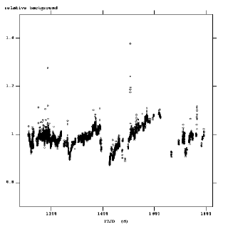
Fig 2 shows the relative background variation determined in the fitting, per pointing, for a typical energy range; the variations are as expected from tracers such as saturated Germanium rates and the general upward trend due to the solar cycle. Discontinuities appear at the times of detector 2 and 17 failures, as expected. Occasional high values are encountered which were not high enough to be removed by the preliminary data filtering, but these are accounted for in the fitting procedure.

Figure 1: Sky distribution of exposure, at 1 MeV. Galactic coordinates centred on $l=b=0$. Units:$10^{7}$ cm² s. Green: 0.5–1.4, yellow: 1.4–4, orange: 4–13, red: 13–35

Figure 2: Time dependence of background for 48 - 58 keV determined from the fitting procedure. Relative units. Time axis in days since 1 Jan 2000

6.2 Spectra

Figure 3: Spectrum of diffuse emission summed over components (blue), and sum of all sources (red), for the inner region of the Galaxy ($330^{\circ}<l<30^{\circ},|b|<10^{\circ}$). 3$\sigma$ source threshold.

Figure 4: Spectrum of diffuse emission summed over model components, for the inner region of the Galaxy ($330^{\circ}<l<30^{\circ},|b|<10^{\circ}$). 3$\sigma$ source threshold. Also shown is the fit of SPI data to power-law plus positronium plus line, using the full energy response. Note that the fit lies below the data points because of the non-diagonal energy reponse of SPI. Magenta point: diffuse emission measured by IBIS/ISGRI (Terrier et al., 2004).

Figure 5: Spectrum of diffuse emission summed over model components, for the central part of the Galaxy ($350^{\circ}<l<10^{\circ},|b|<10^{\circ}$). See Fig 4 caption for details of fit.

Figure 6: Spectrum of diffuse emission summed over model components, for the Galactic-disk region ($330^{\circ}<l<350^{\circ},10^{\circ}<l<30^{\circ},|b|<10^{\circ}$). See Fig 4 caption for details of fit.

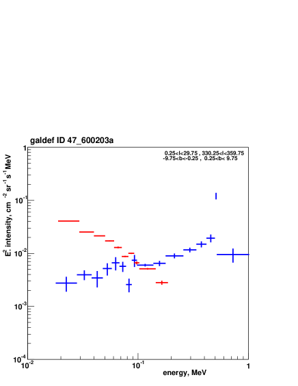
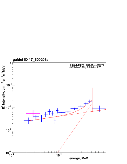
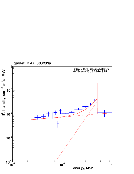
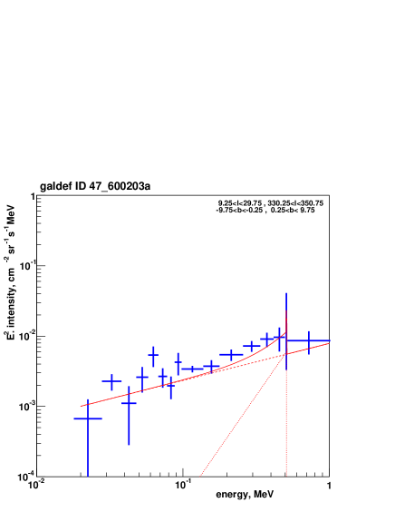
Fig. 3 shows the spectra of the summed catalogue sources and of total diffuse emission, for the inner region of the Galaxy ($330^{\circ}<l<30^{\circ},|b|<10^{\circ}$). We find a clear change from source-dominated to diffuse-dominated emission in the inner Galaxy, going from low to high energies. The transition energy is in the vicinity of 100 keV, but this depends on the fitted sky region due to variation of relative intensities of the components along the plane of the Galaxy. The ‘diffuse’ emission may of course include contributions from unresolved sources.

We have studied the effect of reducing the threshold for sources included in the fit from 3$\sigma$ to 2$\sigma$ and 1$\sigma$. As expected the diffuse component decreases while the source component increases. However the diffuse component decreases by only 30% for the 2$\sigma$ source selection, which is at the lower limit for a plausible cut. For the 1$\sigma$ source selection, the source component shows contamination from the diffuse emission above 100 keV due to ‘cross-talk’ between the components. We adopt the 3$\sigma$ selection as standard in what follows.

The spectra can be fitted by a combination of power-law and the positron annihilation components (positronium continuum with the sharp upper edge at 511 keV and a linear decrease towards lower energies, and the 511 keV line). Fit results for the inner region of the Galaxy ($330^{\circ}<l<30^{\circ},|b|<10^{\circ}$), the central part of the Galaxy ($350^{\circ}<l<10^{\circ},|b|<10^{\circ}$), and the Galactic-disk region ($330^{\circ}<l<350^{\circ},10^{\circ}<l<30^{\circ},|b|<10^{\circ}$)  are given in Table 3. Fig. 4 shows the spectrum in the inner region of the Galaxy ($330^{\circ}<l<30^{\circ},|b|<10^{\circ}$), and Fig. 5 the spectrum for the central part of the Galaxy ($350^{\circ}<l<10^{\circ},|b|<10^{\circ}$). All regions show a hard power law, with spectral index around 1.7.

The positronium edge at 511 keV is highly significant, and below it the positronium continuum with its characteristic linear increase (I=AE) is clearly visible. For the Galactic-disk region ($330^{\circ}<l<350^{\circ},10^{\circ}<l<30^{\circ},|b|<10^{\circ}$), Fig. 6, the positronium component is small and not significant, as expected, and the spectrum is consistent with a power law.

Using the fit results for the central part of the Galaxy ($350^{\circ}<l<10^{\circ},|b|<10^{\circ}$), the 511 keV flux is $0.81\pm 0.07\times 10^{-3}$ cm^-2s^-1, and the 3$\gamma$ continuum flux is $4.15\pm 0.64\times 10^{-3}$ cm^-2s^-1. This gives a positronium fraction $f$ of $0.97-1.08$, consistent with other determinations (Kinzer et al., 2001; Jean et al., 2004; Churazov et al., 2005); although this is not the main goal of this analysis, it provides a consistency check on the analysis methods. While the positronium flux decreases by a factor at least $\sim$7 from $|l|<10^{o}$ to $|l|>10^{o}$, the power-law component decreases by only a factor $\sim 2$. This clearly shows the difference in angular distribution and hence a different spatial origin of the emission.

The power-law continuum flux in this inner region is $1.3\pm 0.25\times 10^{-3}$ cm^-2s^-1 for 300–500 keV, i.e. about 1/3 of the positronium continuum in this range. The positronium component is small in the Galactic-disk region ($330^{\circ}<l<350^{\circ},10^{\circ}<l<30^{\circ},|b|<10^{\circ}$), which allows a more precise determination of the non-positron continuum.

For comparison the low-energy diffuse emission detection by IBIS/ISGRI (Terrier et al., 2004) is also shown in Fig 4 ; the agreement is satisfactory. The SPI spectrum is compared with RXTE, COMPTEL and OSSE results in Fig 7 ; the comparison is made in the region the central part of the Galaxy ($350^{\circ}<l<10^{\circ},|b|<10^{\circ}$), since this is most compatible with the regions reported for RXTE (Revnivtsev, 2003) and OSSE (Kinzer et al., 1999).

Table 3: SPI diffuse emission intensity spectrum fitted to
I(E) = A E^-γ + C E (E$<$0.511) + D$\delta$(E-0.511) cm^-2 sr^-1s^-1 MeV^-1 where E is energy in MeV.

parameter	value	error
$330^{\circ}<l<30^{\circ}$, $|b|<10^{\circ}$
A	8.32 10-3	1.8 10-3
$\gamma$	1.69	0.09
C	1.19 10-1	2.8 10-2
D	2.36 10-3	3.8 10-4
$350^{\circ}<l<10^{\circ}$, $|b|<10^{\circ}$
A	1.15 10-2	2.2 10-3
$\gamma$	1.82	0.08
C	2.61 10-1	4.0 10-2
D	6.62 10-3	5.6 10-4
$330^{\circ}<l<350^{\circ}$, $10^{\circ}<l<30^{\circ}$
$|b|<10^{\circ}$
A	7.87 10-3	2.5 10-3
$\gamma$	1.47	0.14
C	4.49 10-2	3.2 10-2
D	2.70 10-4	4.3 10-4

7 Discussion

7.1 Spectral shape

The OSSE spectrum is somewhat higher than the SPI result in the 20–100 keV range (Fig 7). This suggests that the OSSE result includes significant source contamination, which is better accounted for in the SPI analysis.

The RXTE spectrum is certainly above the extrapolation of the SPI power-law. This suggests a much steeper spectrum below 20 keV, or an additional component with a cutoff around this energy. For RXTE, we use the results of Revnivtsev (2003) since this is probably more free of point-source contamination than e.g. Valinia & Marshall (1998) and Valinia et al. (2000a); however it refers to the region $350^{\circ}<l<10^{\circ},2<|b|<10^{\circ}$ , i.e. avoiding the Galactic ridge itself. The latitude distribution of diffuse emission measured by RXTE is rather broad (Valinia & Marshall, 1998) so the use of this spectrum is appropriate

A rapid softening of the spectrum below the SPI range is indicated by a comparison with XMM and Chandra results. Hands et al. (2004) (XMM) find a total 2–10 keV intensity $9.6\times 10^{-11}$ erg cm^-2 s^-1 deg^-2 for $l=19^{o}-22^{o},|b|\leq 0.5^{o}$, 80% of which is diffuse or at least not in known sources, corresponding to 0.2 MeV cm^-2 s^-1 sr^-1 in the units of Fig 7. Ebisawa et al. (2001, 2005) (Chandra) finds a similar value for diffuse emission at $l=28^{o},b=-0.2^{o}$. Even allowing for the large concentration of the emission to the ridge, this is above the extrapolation of the SPI power-law by at least a factor 3. This is consistent with the inclusion of a cutoff power-law at low energies by Kinzer et al. (1999) in the OSSE analysis. It is also compatible with the steeper power-law (index $>2$) below 20 keV measured by Ginga (Yamasaki et al., 1997).

Figure 7: Comparison of spectrum of diffuse emission (the central part of the Galaxy ($350^{\circ}<l<10^{\circ},|b|<10^{\circ}$)), with other experiments. Data from RXTE (cyan) (Revnivtsev, 2003), SPI (blue) (this work), OSSE (magenta curves) (Kinzer et al., 1999) (their Table 3 and Fig 5, VP 5+16: $l=0,b=0$) , COMPTEL (green) (Strong et al., 1999) and EGRET (red) (Strong et al., 2004b). Note that the RXTE data refer to the region $350^{\circ}<l<10^{\circ},2<|b|<10^{\circ}$ (see text).

Figure 8: Broadband spectrum of diffuse emision ($330^{\circ}<l<30^{\circ},|b|<5^{\circ}$ ), compared with model based on cosmic-ray interactions from Strong et al. (2004b, d). Data from RXTE (cyan), SPI (red lines), IBIS (magenta), COMPTEL (green), (references as in Fig 7) and EGRET (red bars) (Strong et al., 2004b) are shown. Dashed/green curve: inverse Compton,dotted/red: $\pi^{o}$-decay, dashed-dot/light blue: bremsstrahlung, EB: extragalactic background, dark blue: total model. Notes: (a) the RXTE data refer to the region $350^{\circ}<l<10^{\circ},2<|b|<10^{\circ}$ , so this may explain in part the high intensity relative to the SPI results; (b) the EGRET data $>$10 GeV have been corrected for the new sensitivity estimate given by Thompson, Bertsch & O’Neal (2005), which results in higher values than in Strong et al. (2004b); a 50% flux error has been adopted to plot this data.

7.2 Sources: resolved and unresolved

For 20-100 keV the resolved source/diffuse emission ratio is about 10 (Fig 3), which is compatible with existing estimates of the total source emission in the Galaxy: (Grimm et al., 2002) of 2 10³⁹ erg s^-1 and the total diffuse emission of 10³⁸ erg s^-1 (Dogiel et al., 2002a). These estimates are mainly based on the energy range 2–10 keV (largely RXTE-based) so this is only a plausibility check.

It is of interest to estimate the limitations of the present analysis which arise from the SPI instrument itself: the number of sources visible is ultimately limited, at low energies, by source confusion. The SPI angular response has a width of about 2.6^o, which means that for the inner radian in longitude within 5^o of the plane we cannot detect more than $60\times 10/2.6^{2}\sim$100 sources. This limits the flux which could ever be explicitly attributed to detected sources, as follows. From Table 2, using the data between 3$\sigma$ and 10$\sigma$ and the first 6 energy ranges, we find an average logN($>$S)-logS slope of -0.9, i.e. converging to low fluxes. There are 57 sources $>3\sigma$ in 18 – 48 keV in the area chosen above, and from this it follows that we formally have to go down to 1.6$\sigma$ to reach the confusion limit. Integrating N(S)$\times$S, we find that the total source flux increases by about 1.5 going from our adopted 3$\sigma$ (Fig 3) to the confusion limit. This is a very rough estimate, but illustrates that we are near the limit of what could be deduced from the SPI data, and that the total flux in detected sources could never be more than 50% larger than shown in Fig 3.

Sources undetectable because of confusion or low flux will by definition be interpreted as part of the diffuse emission in our analysis. The full analysis must then involve detailed modelling of source populations, which will be addressed in future work.

7.3 Diffuse continuum emission

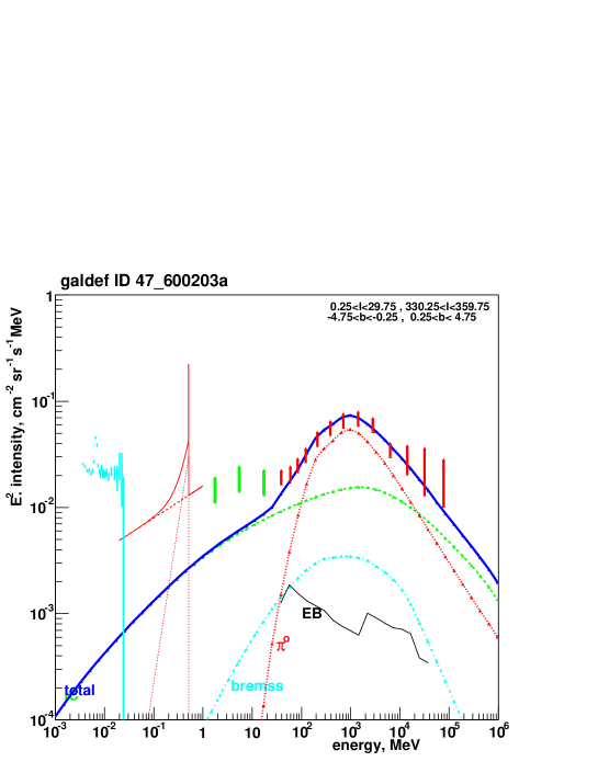
The broad-band spectrum from 2 keV to 100 GeV, including RXTE, SPI, COMPTEL and EGRET, for $330^{\circ}<l<30^{\circ},|b|<5^{\circ}$ is compared with predictions using the galprop model in Fig 8. The RXTE spectrum is for $350^{\circ}<l<10^{\circ},2<|b|<10^{\circ}$ so that its inclusion is only indicative, but illustrates the softening of the spectrum below 20 keV. The model is the ‘optimized’ one from Strong et al. (2004b, d), including the cosmic-ray generated bremsstrahlung and inverse Compton components. Evidently neither of these processes is sufficient to account for the observed non-thermal hard X-ray spectrum; increasing the inverse Compton by invoking a steeper electron spectrum leads to an overprediction of the EGRET data points. Alternative explanations of the hard X-ray spectrum have been mentioned in the Introduction, but these do not easily produce the observed very hard spectrum, so that a population of compact sources seems to us most likely, and anomalous X-ray pulsars (AXPs), with their very hard spectra (Kuiper, Hermsen & Mendez, 2004), appear good candidates. AXPs also have an appropriate young population distribution compatible with the SPI result.

This picture is consistent with a change of origin from truly diffuse emission below 20 keV with a steep spectrum, as seen by RXTE, XMM and Chandra, to a source-dominated origin with a hard spectrum above 20 keV as seen by SPI.

The present work will form the basis for more detailed evaluation of these models.

8 Conclusions

The diffuse continuum emission from the Galactic plane has been detected at high significance with SPI. The positronium and non-thermal components are clearly separated, with the positronium dominating above 300 keV in the inner Galaxy. The contribution from detectable point-sources has for the first time been explicitly accounted for, which was not possible with earlier experiments. The combined emission from detectable sources varies from a factor 10 times the diffuse emission at low energies to negligible at high energies.

Spectral analysis, using the SPI energy response, reveals a power-law component with index about -1.7, consistent with OSSE and COMPTEL results. The positronium flux drops by factor at least 7 from $|l|<10^{o}$ to $|l|>10^{o}$ in accord with other studies. The power-law component by contrast drops by only a factor 2, proving a quite different longitude distribution and spatial origin.

We suggest a change of origin from truly diffuse emission below 20 keV with a steep spectrum, to a source-dominated origin with a hard spectrum above 20 keV.

From the broadband spectrum of the diffuse emision from keV to TeV energies we see that the emission in the SPI range cannot be easily explained as inverse Compton or bremsstrahlung from cosmic-ray electrons. Either another mechanism is at work or there is a new population of compact sources with characteristic high-energy tails.

In view of the apparent difficulty to produce the very hard spectrum with a diffuse mechanism, at present the source population seems the most plausible explanation. Possible candidates are the anomalous X-ray pulsars (AXPs) with the characteristic hardening of their spectra around 100 keV. Detailed evaluation of the contribution from unresolved point-sources will require population synthesis studies, and this will be the subject of future work. Meanwhile we are investigating further the possibility of diffuse mechanisms like that proposed by Dogiel et al. (2002b).

Appendix A Model Fitting Details

The objective of the model fitting analysis is now to extract information about $\theta_{i}$ in the form of posterior probability distributions, and their moments (mean, standard deviation etc) and any other functions of interest (e.g. the total image).

Fitting and error estimation

The likelihood function is:

$$L(D|\bar{\theta})=\prod_{k}e^{-d_{k}}d_{k}^{n_{k}}/n_{k}!$$

where $n_{k}$ are the measured data (denoted collectively by $D$).

and the posterior probability $P(\bar{\theta}|D)$ is expressed in terms of the likelihood and the prior probability $Pr(\bar{\theta})$ using Bayes theorem:

$$P(\bar{\theta}|D)=L(D|\bar{\theta})Pr(\bar{\theta})/P(D)$$

The posterior for one parameter is obtained by marginalizing over the other parameters:

$$P(\theta_{i}|D)=\int_{i^{\prime}\neq i}P(\bar{\theta}_{i}^{\prime}|D)d^{N}\theta^{\prime}$$

and its mean value is

$$<\theta_{i}|D>=\int\theta_{i}P(\theta_{i}|D)d\theta_{i}=\int\theta_{i}P(\bar{\theta}|D)d^{N}\theta$$

with standard deviation

$$\Delta\theta_{i}|D=sqrt\int(\theta_{i}-<\theta_{i}|D>)^{2}P(\theta_{i}|D)d\theta_{i}$$

$$=sqrt\int(\theta_{i}-<\theta_{i}|D>)^{2}P(\bar{\theta}|D)d^{N}\theta$$

An analytical approximation to the covariance matrix and hence the error estimates can be obtained by expressing the log-likelihood function as an expansion about the maximum:

$$\log L(\bar{\theta})=\log L(\bar{\theta}_{o})+{1\over 2}\Sigma_{p}\Sigma_{q}(\theta_{p}-\theta_{p}^{o})(\theta_{q}-\theta_{q}^{o})H_{pq}$$

where the Hessian matrix is $H_{pq}=\partial^{2}\log L/\partial\theta_{p}\partial\theta_{q}$. The marginalization integration can then be done analytically using diagonalization (Sivia (1997): Ch 3.2 and Appendix A.3) which gives the result for the covariance under the posterior:

$$\sigma_{pq}^{2}=<(\theta_{p}-\theta_{p}^{o})(\theta_{q}-\theta_{q}^{o})>=H_{pq}^{-1}$$

The inverse of $H$ can be written in terms of the matrix of eigenvectors $X$ and eigenvalues $\Lambda=diag(\lambda_{q})$ :

$$HX=X\Lambda$$

$$X=H^{-1}X\Lambda$$

$$H^{-1}=X\Lambda^{-1}X^{-1}=X\Lambda^{-1}X^{T}$$

since eigenvectors of a real symmetric matrix are orthogonal, $X^{-1}=X^{T}$. For a single parameter,

$$\sigma_{pp}^{2}=<(\theta_{p}-\theta_{p}^{o})^{2}>=H_{pp}^{-1}=(X\Lambda^{-1}X^{T})_{pp}=\Sigma_{q}{X_{pq}^{2}\over\lambda_{q}}$$

It is interesting to note that a completely different formalism involving the distribution of the maximum-likelihood ratio (Strong, 1985) and maximizing the likelihood under constraints instead of marginalizing over unwanted parameters, actually leads to the same formula for errors on one parameter, once we express the inverse Hessian in terms of eigenvalues. This has not been noted before to the author’s knowledge. One advantage of the Bayes formalism is that the covariances can be used to compute the errors on linear combinations of components.

The RMS error on a linear combination of parameters is directly related to the covariances as follows

$$f=\Sigma w_{i}\theta_{i}$$

$$\Delta f=w_{i}\Delta\theta_{i}$$

$$(\Delta f)^{2}=\Sigma_{i}\Sigma_{j}w_{i}w_{j}\Delta\theta_{i}\Delta\theta_{j}$$

$$<(\Delta f)^{2}>=\Sigma_{i}\Sigma_{j}w_{i}w_{j}<\Delta\theta_{i}\Delta\theta_{j}>$$

$$=\Sigma_{i}\Sigma_{j}w_{i}w_{j}\sigma_{ij}^{2}$$

Appendix B Fit results

This appendix consists of Tables B1–4, containing all the SPI results plotted in the spectra, to enable convenient use of the present work.

Table 4: SPI diffuse emission spectrum for various source variability timescales. * indicates selected sources (Sco X-1, 4U1700-377, OAO 1657-4154) allowed to vary on timescale of SPI pointings.
$0.25^{\circ}<l<29.75^{\circ},330.25^{\circ}<l<359.75^{\circ}$,
$-9.75^{\circ}<b<-0.25^{\circ},0.25^{\circ}<b<9.75^{\circ}$

Energy range	variability	intensity	error	ID
(keV)	timescale	cm-2 sr-1
	(days)	s-1 MeV-1
18.0- 28.0	const	5.469	1.711	2481
18.0- 28.0	200	4.484	1.580	2501
18.0- 28.0	100	3.572	1.452	2502
18.0- 28.0	50	2.870	1.369	2503
18.0- 28.0	*	4.341	2.496	2505
28.0- 38.0	const	3.725	0.782	2482
28.0- 38.0	200	3.112	0.694	2511
28.0- 38.0	100	2.846	0.656	2512
28.0- 38.0	50	2.626	0.629	2513
28.0- 38.0	*	3.295	0.723	2515
38.0- 48.0	const	1.894	0.643	2483
38.0- 48.0	200	1.861	0.421	2521
38.0- 48.0	100	1.783	0.410	2522
38.0- 48.0	50	1.778	0.413	2523
38.0- 48.0	*	1.826	0.417	2525
48.0- 58.0	const	1.859	0.483	2484
48.0- 58.0	200	1.958	0.923	2531
48.0- 58.0	100	1.977	0.930	2532
48.0- 58.0	50	1.786	0.904	2533
48.0- 58.0	*	1.755	0.769	2535
58.0- 68.0	const	1.685	0.469	2485
58.0- 68.0	200	1.643	0.466	2541
58.0- 68.0	100	1.602	0.461	2542
58.0- 68.0	50	1.559	0.459	2543

Table 5: SPI diffuse emission spectrum for
$330^{\circ}<l<30^{\circ}$, $|b|<10^{\circ}$

Energy range	components	intensity	error	ID
(keV)		cm-2 sr-1
		s-1 MeV-1
18.0- 28.0	1-9	5.469	1.711	2481
28.0- 38.0	1-9	3.725	0.782	2482
38.0- 48.0	1-9	1.894	0.643	2483
48.0- 58.0	1-9	1.859	0.483	2484
58.0- 68.0	1-9	1.685	0.469	2485
68.0- 78.0	1-9	1.077	0.232	2486
78.0- 88.0	1-9	0.378	0.110	2487
88.0- 98.0	1-9	0.863	0.220	2488
98.0- 138.0	1-9	0.444	0.024	2489
138.0- 178.0	1-9	0.265	0.030	2490
178.0- 258.0	1-9	0.196	0.020	2291
258.0- 338.0	1-9	0.134	0.013	2248
338.0- 418.0	1-9	0.106	0.014	2249
418.0- 498.0	1-9	0.093	0.016	2183
508.0- 514.0	1-9	0.465	0.064	2207
518.0-1018.0	1-9	0.018	0.005	2186

Table 6: SPI total source emission spectrum for
$330^{\circ}<l<30^{\circ}$, $|b|<10^{\circ}$

Energy range	components	intensity	error	ID
(keV)		cm-2 sr-1
		s-1 MeV-1
18.0- 28.0	10-132	64.054	0.630	2481
28.0- 38.0	10-132	18.619	0.161	2482
38.0- 48.0	10-106	9.585	0.095	2483
48.0- 58.0	10-71	5.004	0.116	2484
58.0- 68.0	10-53	2.707	0.108	2485
68.0- 78.0	10-45	1.579	0.036	2486
78.0- 88.0	10-50	1.198	0.029	2487
88.0- 98.0	10-39	0.770	0.047	2488
98.0- 138.0	10-32	0.379	0.012	2489
138.0- 178.0	10-21	0.114	0.010	2490

Table 7: SPI diffuse emission spectrum for
$0.25^{\circ}<l<9.75^{\circ}$, $350.25^{\circ}<l<359.75^{\circ}$, $-9.75^{\circ}<b<-0.25^{\circ}$, $0.25^{\circ}<b<9.75^{\circ}$ .

Energy range	components	intensity	error	ID
(keV)		cm-2 sr-1
		s-1 MeV-1
18.0- 28.0	1-9	13.829	3.434	2481
28.0- 38.0	1-9	7.015	1.402	2482
38.0- 48.0	1-9	4.502	1.065	2483
48.0- 58.0	1-9	3.754	0.858	2484
58.0- 68.0	1-9	2.335	0.680	2485
68.0- 78.0	1-9	2.217	0.442	2486
78.0- 88.0	1-9	0.574	0.173	2487
88.0- 98.0	1-9	1.599	0.376	2488
98.0- 138.0	1-9	0.825	0.037	2489
138.0- 178.0	1-9	0.492	0.043	2490
178.0- 258.0	1-9	0.359	0.028	2291
258.0- 338.0	1-9	0.237	0.019	2248
338.0- 418.0	1-9	0.190	0.019	2249
418.0- 498.0	1-9	0.190	0.022	2183
508.0- 514.0	1-9	1.244	0.095	2207
518.0-1018.0	1-9	0.022	0.008	2186

Table 8: SPI diffuse emission spectrum for
$9.25^{\circ}<l<29.75^{\circ}$, $330.25^{\circ}<l<350.75^{\circ}$, $-9.75^{\circ}<b<-0.25^{\circ}$, $0.25^{\circ}<b<9.75^{\circ}$

Energy range	components	intensity	error	ID
(keV)		cm-2 sr-1
		s-1 MeV-1
18.0- 28.0	1-9	1.331	1.179	2481
28.0- 38.0	1-9	2.147	0.564	2482
38.0- 48.0	1-9	0.610	0.455	2483
48.0- 58.0	1-9	0.936	0.369	2484
58.0- 68.0	1-9	1.363	0.441	2485
68.0- 78.0	1-9	0.503	0.154	2486
78.0- 88.0	1-9	0.286	0.101	2487
88.0- 98.0	1-9	0.494	0.173	2488
98.0- 138.0	1-9	0.252	0.027	2489
138.0- 178.0	1-9	0.152	0.033	2490
178.0- 258.0	1-9	0.119	0.022	2291
258.0- 338.0	1-9	0.083	0.015	2248
338.0- 418.0	1-9	0.064	0.015	2249
418.0- 498.0	1-9	0.046	0.017	2183
508.0- 514.0	1-9	0.085	0.072	2207
518.0-1018.0	1-9	0.016	0.006	2186