Spherical Isothermal Self-Similar Shock Flows

Abstract

We explore self-similar dynamical processes in a spherical isothermal self-gravitational fluid with an emphasis on shocks and outline astrophysical applications of such shock solutions. The previous similarity shock solutions of Tsai & Hsu and of Shu et al. may be classified into two types: Class I solutions with downstream being free-fall collapses and Class II solutions with downstream being Larson-Penston (LP) type solutions. By the analyses of Lou & Shen and Shen & Lou, we further construct similarity shock solutions in the ‘semi-complete space’. These general shock solutions can accommodate and model dynamical processes of radial outflows (wind), inflows (accretion or contraction), subsonic oscillations, and free-fall core collapses all with shocks in various settings such as star-forming molecular clouds, ‘champagne flows’ in HII regions around luminous massive OB stars or surrounding quasars, dynamical connection between the asymptotic giant branch phase to the proto-planetary nebula phase with a central hot white dwarf as well as accretion shocks around compact objects such as white dwarfs, neutron stars, and supermassive black holes. By a systematic exploration, we are able to construct families of infinitely many discrete Class I and Class II solutions matching asymptotically with a static outer envelope of singular isothermal sphere; the shock solutions of Tsai & Hsu form special subsets. These similarity shocks travel at either subsonic or supersonic constant speeds. We also construct twin shocks as well as an ‘isothermal shock’ separating two fluid regions of two different yet constant temperatures.

1 Introduction

Self-gravitational inflows (contractions or accretions or collapses) and outflows (expansions or winds) of an isothermal fluid with spherical symmetry have been investigated over the past several decades in various astrophysical contexts (e.g., star formations, supernova explosions, formation and evolution of galaxy clusters etc). When a fluid system is sufficiently away from initial and boundary conditions, it may evolve into self-similar behaviours (e.g., Sedov 1959; Landau & Lifshitz 1959). Under isothermal condition and spherical symmetry, Larson (1969a,b) and Penston (1969a,b) independently found self-similar solutions, now commonly referred to as Larson-Penston (LP) type solutions. Shu (1977) obtained another class of similarity solutions containing the so-called ‘expansion wave collapse solution’ (EWCS) that describes an expanding region of core collapse from a surrounding molecular cloud. In addition to these solutions, Hunter (1977) derived a class of discrete similarity solutions in the ‘complete solution space’ from $t\rightarrow-\infty$ to $t\rightarrow+\infty$. These solutions may represent clouds which are accreted to a central mass point as an inward propagating compression wave driven by external gas pressure. Whitworth & Summers (1985) expanded the solution space by introducing a bounded two-parameter continuum {$z_{0}$, $w_{0}$} to the known discrete solutions. The two parameters $z_{0}$ and $w_{0}$ correspond to $\alpha_{0}$ and $m_{0}$ in the solutions of Shu (1977), which characterize the asymptotic solution forms as $t\rightarrow-\infty$ and $t\rightarrow+\infty$ respectively. Hunter (1986) noted that the additional bands of solutions of Whitworth & Summers (1985) involve weak discontinuities across the sonic critical line (Boily & Lynden-Bell 1995) and may be unstable to perturbations (e.g., Lazarus 1981). Generalizing these earlier results, Lou & Shen (2004) recently obtained a new class of self-similar isothermal solutions, referred to as ‘envelope expansion with core collapse’ (EECC) solutions, which are characterized by an interior free-fall collapse towards the core with an exterior envelope expanding at a constant radial speed at large radii. A broad class of EECC solutions without crossing the sonic critical line can be readily obtained; meanwhile, a special class of infinitely many discrete EECC solutions crossing the sonic critical line twice analytically can also be constructed. Boily & Lynden-Bell (1995) and Murakami et al. (2004) studied self-similar solutions for spherical collapses with radiative effects included. The work of Fatuzzo et al. (2004) treated protostellar collapse in a polytropic gaseous sphere and found self-similar solutions with nonzero inward speed at large radii (see earlier emphasis of Shen & Lou 2004 on this point); in their model consideration, the infall rates are determined by the inward speed $v_{\infty}$, the overdensity $\Lambda$, the polytropic index $\Gamma$ for the background equation of state, and the polytropic index $\gamma$ for the dynamic equation of state; they did not explore polytropic solutions crossing the sonic critical line.

Based on prior results, Tsai & Hsu (1995) found two classes of isothermal self-similar shock solutions referred to as Class I and II solutions which connects a static singular isothermal sphere (SIS) envelope to a free-fall solution and a LP solution respectively (see § 3.1.1). Shu et al. (2002) expanded Tsai & Hsu’s LP similarity shock solution to model the so-called ‘champagne flows’ driven by a shock into HII regions surrounding luminous massive OB stars (see § 3.1.2). Further extending the work of Tsai & Hsu (1995) and Shu et al. (2002), Shen & Lou (2004) introduced Class I shock solutions for dynamical evolution of young stellar objects and Class II solutions to model ‘champagne flows’ of HII regions surrounding OB stars. More generally, they pointed out that shock similarity solutions can be matched with various types of upstream solutions (see § 3.1.3).

In this paper, we construct self-similar isothermal shock solutions by exploring diverse possibilities. In § 2, we summarize the basic isothermal fluid equations, the self-similar transformation and the isothermal shock conditions. In reference to previous similarity shock solutions, we derive in § 3 an infinite number of discrete shock solutions for Class I and Class II categories by exploring the $\alpha-v$ phase diagram and present new similarity shock solutions: twin shock solution and two-temperature flows separated by shocks. In § 4, we discuss astrophysical applications of these shock solutions. In § 5, we summarize and discuss our results.

2 Formulation of Shock Conditions

We begin with the fluid equations in the Eulerian form in the spherical polar coordinates $(r,\theta,\phi)$. By spherical symmetry, the mass conservation is given by

$$\frac{\partial M}{\partial t}+u\frac{\partial M}{\partial r}=0\ ,\qquad\qquad\hskip 14.22636pt\frac{\partial M}{\partial r}=4\pi r^{2}\rho\ ,$$ (1)

where $M(r,t)$ is the enclosed mass within radius $r$ at time $t$. The equivalent form of continuity equation (1) is simply

$$\frac{\partial\rho}{\partial t}+\frac{1}{r^{2}}\frac{\partial}{\partial r}(r^{2}\rho u)=0\ ,$$ (2)

where $\rho$ is the gas mass density and $u$ is the radial flow speed. The radial momentum equation reads

$$\frac{\partial u}{\partial t}+u\frac{\partial u}{\partial r}=-\frac{a^{2}}{\rho}\frac{\partial\rho}{\partial r}-\frac{GM}{r^{2}}\ ,$$ (3)

where $G\equiv 6.67\times 10^{-8}$ dyn cm² g^-2 is the gravitational constant, $a\equiv(p/\rho)^{1/2}$ is the isothermal sound speed and $p$ is the gas pressure. The Poisson equation is automatically satisfied by equations (1) and (3).

The dimensionless independent similarity variable is $x=r/(at)$ and the similarity transformations are

$$\qquad\rho(r,t)=\frac{\alpha(x)}{4\pi Gt^{2}}\ , \hskip 8.5359ptM(r,t)=\frac{a^{3}t}{G}m(x)\ ,$$

$$\qquad u(r,t)=av(x)\ , \hskip 8.5359pt\Phi(r,t)=a^{2}\phi\ ,$$ (4)

where $\alpha(x)$, $m(x)$ and $v(x)$ are dimensionless reduced variables for mass density $\rho(r,t)$, enclosed mass $M(r,t)$ and radial flow speed $u(r,t)$, respectively; $\Phi$ is the gravitational potential such that $-\partial\Phi/\partial r=-GM(r,t)/r^{2}$ and $\phi(x)$ is its reduced form. These reduced variables depend only on $x$ (e.g., Shu 1977; Lou & Shen 2004).

Transformation (4) and equation (1) lead to

$$m+(v-x)\frac{\hbox{d}m}{\hbox{d}x}=0\ ,\qquad\hskip 14.22636pt\frac{\hbox{d}m}{\hbox{d}x}=x^{2}\alpha\ ,$$ (5)

which gives $m(x)$ in terms of $x$, $v$ and $\alpha$, namely

$$m(x)=x^{2}\alpha(x-v)\ .$$ (6)

The physical requirement of a positive $m(x)$ corresponds to the solution regime of $x-v>0$.

By transformation (4) and solution (6) in equations (2) and (3), we obtain a pair of coupled nonlinear ordinary differential equations (ODEs):

$$[(x-v)^{2}-1]\frac{\hbox{d}v}{\hbox{d}x}=\left[\alpha(x-v)-\frac{2}{x}\right](x-v)\ ,$$ (7)

$$[(x-v)^{2}-1]\frac{1}{\alpha}\frac{\hbox{d}\alpha}{\hbox{d}x}=\left[\alpha-\frac{2}{x}(x-v)\right](x-v)\ ,$$ (8)

[see eqs (11) and (12) of Shu (1977) and eqs (9) and (10) in Lou & Shen (2004)]. In the two nonlinear ODEs, the critical line is characterized by $(x-v)^{2}-1=0$ and $\alpha=2/x$.

The analytical asymptotic solutions of ODEs (7) and (8) are shown below (see Lou & Shen 2004 for details).

(i) For $x\rightarrow+\infty$, the leading order terms are

$$v\rightarrow V\ ,\qquad\hskip 14.22636pt\alpha\rightarrow\frac{A}{x^{2}}\ ,\qquad\hskip 14.22636ptm\rightarrow Ax\ ,$$ (9)

where $V$ and $A$ are two independent constants, referred to as velocity and mass parameters, respectively. The envelope expansion approaches a constant speed $V$ at large radii.

(ii) For $x\rightarrow 0^{+}$, the leading terms are

$$v\rightarrow-\left(\frac{2m_{0}}{x}\right)^{1/2}\ ,\hskip 5.69046pt\alpha\rightarrow\left(\frac{m_{0}}{2x^{3}}\right)^{1/2}\ ,\hskip 5.69046ptm\rightarrow m_{0}$$ (10)

describing a central free-fall collapse with a constant dimensionless parameter $m_{0}$ for central mass accretion rate (Shu 1977; Lou & Shen 2004; Shen & Lou 2004; Yu & Lou 2005).

For the central LP-type solutions as $x\rightarrow 0^{+}$, the leading order terms are

$$v\rightarrow\frac{2}{3}x\ ,\qquad\hskip 5.69046pt\alpha\rightarrow B\ ,\qquad\hskip 5.69046ptm\rightarrow Bx^{3}/3$$ (11)

with a finite reduced central mass density $B$.

(iii) Along the sonic critical line, the two eigensolutions are respectively

$$-v(x)=(1-x_{\ast})+\left(\frac{1}{x_{\ast}}-1\right)(x-x_{\ast})+\cdots\ ,$$

$$\alpha(x)=\frac{2}{x_{\ast}}-\frac{2}{x_{\ast}}\left(\frac{3}{x_{\ast}}-1\right)(x-x_{\ast})+\cdots$$ (12)

for type 1 solutions, and

$$-v(x)=(1-x_{\ast})-\frac{1}{x_{\ast}}(x-x_{\ast})+\cdots\ ,$$

$$\alpha(x)=\frac{2}{x_{\ast}}-\frac{2}{x_{\ast}^{2}}(x-x_{\ast})+\cdots$$ (13)

for type 2 solutions, as defined by Shu (1977) and used in the subsequent work [e.g. Hunter (1977); Whitworth & Summers (1985); Lou & Shen (2004); Shen & Lou (2004)]. These analytical asymptotic solutions provide necessary starting conditions for a fourth-order Runge-Kutta integration scheme (Press et al. 1986) to obtain global solutions numerically. We derive various classes of numerical solutions from the two coupled nonlinear ODEs (7) and (8) globally.

For an isothermal gas, cooling effects by dust grains allow efficient radiation of compressional heat generated during a collapse. The energy conservation involves radiative losses (e.g., Courant & Friedrichs 1976; Spitzer 1978). Under the isothermal approximation, we need to consider conservations of mass and momentum across a shock, namely

$$\rho_{d}(u_{d}-u_{s})=\rho_{u}(u_{u}-u_{s})\ ,$$ (14)

$${a_{d}}^{2}\rho_{d}+\rho_{d}u_{d}(u_{d}-u_{s})=a_{u}^{2}\rho_{u}+\rho_{u}u_{u}(u_{u}-u_{s})\ ,$$ (15)

where $u$, $a$ and $\rho$ are the radial gas flow speed, the isothermal sound speed and the mass density, respectively, and subscripts d (u) denote the downstream (upstream) of a shock, $u_{s}=a_{d}x_{sd}=a_{u}x_{su}=r_{s}/t$ is the outward moving speed of the shock with $r_{s}$ being the shock radius. Using dimensionless reduced variables $v(x)$, $x$, and $\alpha(x)$ to replace $u(r,t)$ and $\rho(r,t)$, we derive the isothermal shock jump conditions in terms of $v(x)$, $x$, and $\alpha(x)$, namely

$$\alpha_{d}(v_{d}-x_{sd})a_{d}=\alpha_{u}(v_{u}-x_{su})a_{u}\ ,$$ (16)

$${a_{d}}^{2}\alpha_{d}+{a_{d}}^{2}\alpha_{d}v_{d}(v_{d}-x_{sd})={a_{u}}^{2}\alpha_{u}+{a_{u}}^{2}\alpha_{u}v_{u}(v_{u}-x_{su})\ .$$ (17)

For an isothermal sound speed ratio $\tau=a_{d}/a_{u}$ and $\tau x_{sd}=x_{su}$, we derive

$$v_{d}-x_{sd}-\tau(v_{u}-x_{su})=(\tau v_{d}-v_{u})(v_{u}-x_{su})(v_{d}-x_{sd})\ ,$$ (18)

$$\alpha_{d}/\alpha_{u}=(v_{u}-x_{su})/[\tau(v_{d}-x_{sd})]\$$ (19)

(Shen & Lou 2004). For $\tau=1$, eqns (18) and (19) become

$$(v_{u}-x_{s})(v_{d}-x_{s})=1$$ (20)

$$\alpha_{d}/\alpha_{u}=(v_{u}-x_{s})/(v_{d}-x_{s})\ ,$$ (21)

where $x_{s}=x_{su}=x_{sd}$ is the reduced shock speed.

Our main goal is to solve coupled nonlinear ODEs (7) and (8) and to apply the jump conditions across various shocks to match with reasonable boundary conditions for constructing global similarity shock solutions. Conceptually, this would help to conceive various possible scenarios involving shocks. With proper adaptations, this would lead to interesting physical models for various astrophysical systems.

3 Self-Similar Shock Solutions

We can construct various similarity solutions from nonlinear ODEs (7) and (8) with shocks satisfying shock jump conditions (18) and (19) to match with different analytical asymptotic solutions. In general, these similarity solutions can describe radial outflows (expansions or winds), inflows (contractions or accretions), oscillations, free-fall collapses with one or more shocks. We explore the range of the independent similarity variable $x$ in the ‘semi-complete space’, i.e., from $x\rightarrow 0^{+}$ to $x\rightarrow+\infty$. By the invariant property for the time reversal of the equations, it is easy to establish the correspondence between solutions in the ‘complete solution space’ (Hunter 1977) and solutions in the ‘semi-complete solution space’ (Lou & Shen 2004).

In this section, we first review earlier results of Tsai & Hsu (1995), Shu et al. (2002) and Shen & Lou (2004). We then derive two classes of infinitely many discrete shock solutions including the twin shock solutions. Finally, we study shock solutions with the shock separating the flows of two different yet constant temperatures.

3.1 Previous Shock Solution Results

We now review the similarity solution structure in reference to earlier results of Tsai & Hsu (1995), Shu et al. (2002), and Shen & Lou (2004). The common feature of these shock solutions is that they have been constructed with $\tau=1$ and contain only one shock. As $x\rightarrow 0^{+}$, these shock solutions can match with inner free-fall collapses across the sonic critical line or with inner LP solutions, while as $x\rightarrow+\infty$, they match with the analytical asymptotic solution (i) by equation (9). These solutions can be broadly classified by their behaviours near $x\rightarrow 0^{+}$ into two types: Class I whose downstream solutions are free-fall collapses and Class II whose downstream solutions are LP-type solutions.

3.1.1 Shock Solutions of Tsai & Hsu (1995)

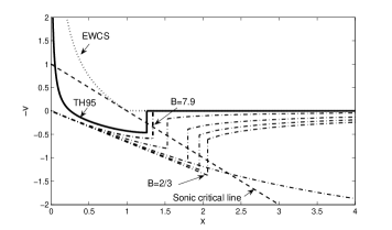
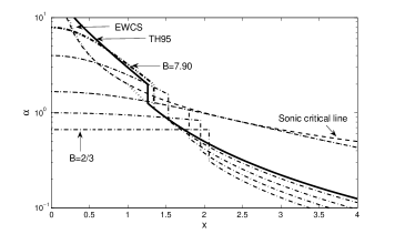
Figure 1: The reduced radial speed $-v(x)$ in linear scale (upper panel) and the reduced mass density $\alpha(x)$ in logarithmic scale (lower panel) versus $x$ in linear scale; the dashed curves correspond to the sonic critical line, the dotted curves correspond to the EWCS of Shu (1977), the heavy solid curve and the heavy dash-dotted curve of Tsai & Hsu (1995) correspond to the shock solutions matching with the inner free-fall collapses and with inner LP-type solutions to a static SIS envelope respectively, the inner free-fall solution crosses the sonic critical line at $x_{\ast}=0.0554$ and the $B$ parameter of the inner LP solution is $B=7.90$; the light dash-dotted curves are solutions with asymptotic breezes at large $x$ found by Shu et al. (2002) with the different curves from top to bottom corresponding to the parameter $B=2/3$, 1, 1.67 and 4 respectively in both upper and lower panels.

Shu (1977) obtained the EWCS (the dotted curve in Figs. 1) with the mass density parameter $A\rightarrow 2^{+}$ and the velocity parameter $V=0$ in equation (9), and the solution touches the sonic critical line at $x_{\ast}=1$ with $m_{0}=0.975$. Tsai & Hsu (1995) considered a self-similar shock travelling into a static SIS envelope with $\tau=1$, $x_{sd}=x_{su}=x_{s}$, $v_{u}=0$ and $\alpha_{u}=2/x_{s}^{2}$, such that the shock jump conditions (20) and (21) appear in the form of

$$v_{d}=x_{s}-\frac{1}{x_{s}}\ ,\qquad\qquad\hskip 8.5359pt\alpha_{d}=2\ .\quad$$ (22)

They showed two specific examples for the two classes of similarity shock solutions: Class I solution given by heavy solid curves in the two panels of Fig. 1 and Class II solution given by heavy dashed-dotted curves in the two panels of Fig. 1. This Class I solution crosses the sonic critical line at $x_{\ast}=0.0554$ and the shock location is at $x_{s}=1.26$ for an outgoing shock travelling at a constant speed of 1.26 times the sound speed $a$. As this Class I solution connects the inner free-fall collapse through an expansion into a static SIS envelope by a shock, the solution has the same properties of the EWCS such that the outer gas envelope remains static with a $r^{-2}$ density profile at large radii and the central gas falls towards the core at a constant rate $m_{0}=0.105$ with a $r^{-3/2}$ density profile and a $r^{-1/2}$ velocity profile. The central mass accretion rate $\dot{M}=m_{0}a^{3}/G$ in this similarity shock solution is a factor of $\sim 0.1$ that predicted by the EWCS of Shu (1977). For the Class II solution, a central expansion with a finite central density (LP solution) matches to a static SIS envelope across a shock; it shows a higher shock speed and strength. The shock location is at $x_{s}=1.34$ for a constant shock expansion speed of $1.34$ times the sound speed $a$ and a reduced core density $B\cong 7.9$.

3.1.2 Shock Solutions of Shu et al. (2002)

Shu et al. (2002) extended the Class II solution of Tsai & Hsu (1995) and used these solutions to model ‘champagne flows’ of HII regions surrounding massive OB stars. By varying the $B$ parameter with fixed $V=0$, they obtained a class of outflow solutions and found both shock speed and strength decreasing with increasing $B$. In Fig. 1, we plot different solutions (dash-dotted curves) with different reduced central density parameter $B=2/3,\ 1,\ 1.67,\ 4,\ 7.90$, corresponding to the mass parameter $A=1.09,\ 1.28,\ 1.52,\ 1.832,\ 2.0$ respectively, and also corresponding to the shock location $x_{s}=2.06,\ 1.95,\ 1.80,\ 1.53,\ 1.34$, respectively. As $B\rightarrow 0^{+}$ (e.g., $B=10^{-6}$) numerically, the mass parameter $A$ also approaches $0^{+}$, and the reduced speed $v(x)$ converges to an invariant form with an invariant fastest and strongest shock solution where the shock is located at $x_{s}=2.56$ (see the heavy solid curve in Fig. 3).

3.1.3 Shock Solutions of Shen & Lou (2004)

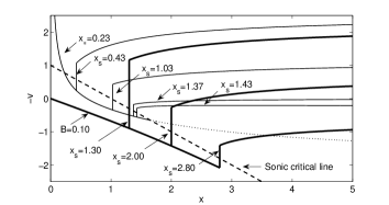
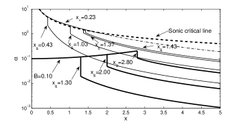
Figure 2: The dimensionless negative reduced radial speed $-v(x)$ (top panel) and reduced mass density $\alpha(x)$ (bottom panel) versus $x$. The dashed lines in both panels are the sonic critical line; the light solid curves are illustrating examples of Class I solutions with the downstream solution crossing the sonic critical line at $x_{\ast}=0.23$ and the shock location $x_{s}$ at $0.43,\ 1.03,\ 1.37,\ 1.43$, respectively; the heavy solid curves are illustrating examples of Class II solutions with the reduced density of the central core $B=0.1$ and the shock location $x_{s}$ at 1.30, 2.00 and 2.80, respectively.

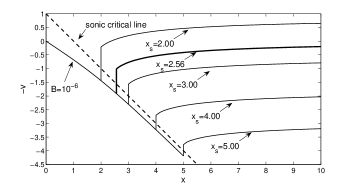
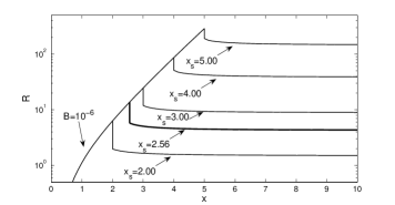
Figure 3: The dimensionless reduced speed $v(x)$ (top panel) and a scaled reduced mass density $R(x)$ where $R(x)\equiv x^{2}\alpha(x)/B$ (bottom panel) versus $x$. The dashed lines are the sonic critical line; the solid curves are the family of Class II solutions in the invariant form with the reduced density of the central core $B\rightarrow 0^{+}$ (viz., $B=10^{-6}$); the heavy solid line is the so-called ‘champagne breeze’ solution of Shu et al. (2002).

By constructing a new family of Class I similarity shock solutions to match with various asymptotic flows, Shen & Lou (2004) modelled (light solid lines in Fig. 2) the dynamical evolution of young stellar objects such as the Bok globule B335 system to account better for the observationally inferred density and velocity profiles as well as the central mass accretion rate. The downstream is part of CP 1 solution for an envelope expansion with core collapse (EECC; Shen & Lou 2004); this EECC solution crosses twice the sonic critical line (viz., $x-v=1$ and $\alpha=2/x$) at $x_{\ast}=0.23$ and $x_{\ast}=1.65$ analytically. By choosing different shock locations $x_{s}=0.43,\ 1.03,\ 1.37,\ 1.43$ as in Fig. 2, we readily construct various upstream solutions to match with the analytical asymptotic solutions at $x\rightarrow+\infty$ (see Table 1 of Shen & Lou 2004). Comparing with Shu et al. (2002), Shen & Lou (2004) significantly broadened the Class II solutions (Fig. 3) for possible ‘champagne flows’ of HII regions around luminous OB stars by allowing for flows at large $x$. The upstream solutions in Shen & Lou (2004) are not limited to the static SIS envelope or ‘champagne breeze’ ($V=0$); by adjusting shock locations (or equivalently, shock speed), it is possible to match with either asymptotic outflow (expansion or wind) solutions ($V>0$) or asymptotic inflow (contraction or accretion) solutions ($V<0$).

3.2 Similarity Shocks into a Static SIS Envelope

Table 1: Class I and II similarity shock solutions matched with a static SIS envelope

description	$m_{0}$	$x_{s}$	$v_{d}$	$\alpha_{d}$	$v_{u}$	$\alpha_{u}$	node
$x_{\ast}(1)=0.0544$	0.105	1.26	0.466	2.00	0	1.26	1
$x_{\ast}(1)=4.75\times 10^{-4}$	$9.42\times 10^{-4}$	0.64	-0.270	3.78	0.459	3.13	2
$x_{\ast}(1)=5.00\times 10^{-5}$	$9.36\times 10^{-5}$	1.04	0.122	2.00	0	1.85	3
$x_{\ast}(1)=6.50\times 10^{-8}$	$1.30\times 10^{-7}$	0.98	-0.0227	2.04	-0.0205	2.03	4
$B=7.90$	-	1.34	0.586	2.00	0	1.12	0
$B=930$	-	0.63	-0.275	3.85	-0.471	3.17	1
$B=9.50\times 10^{4}$	-	1.04	0.0841	2.00	0	1.85	2
$B=1.10\times 10^{7}$	-	0.97	-0.0338	2.07	-0.0349	2.06	3

Columns 1 through 8 provide properties of solutions ($x_{\ast}$ for Class I solutions and $B$ for Class II solutions); reduced central mass accretion rate $m_{0}$ for Class I solutions; the shock location $x_{s}$; the downstream velocity $v_{d}$; the downstream density $\alpha_{d}$; the upstream velocity $v_{u}$, the upstream density $\alpha_{u}$ and the number of stagnation points.

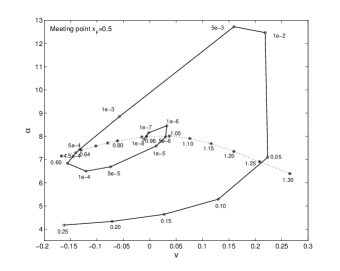
Figure 4: The phase diagram of $\alpha$ versus $v$ at the meeting point $x_{\rm F}=0.5$. Each open circle symbol indicates an integration from $x_{\ast}$ with its value shown explicitly and each asterisk symbol indicates an integration from the shock location $x_{s}$ with its value also shown explicitly. The solid and dotted curves intersect; here we only show four intersections, from right to left, corresponding to four pairs of {$x_{\ast}(1)$, $x_{s}$} as {0.0554, 1.26}, {$5.00\times 10^{-5},1.04$}, {$6.50\times 10^{-8}$, 0.980} and {$4.75\times 10^{-4}$, 0.640}, respectively. The trend of each curve suggests that there may exist an infinite number of discrete Class I shock solutions matched with a static SIS envelope with $A=2$.

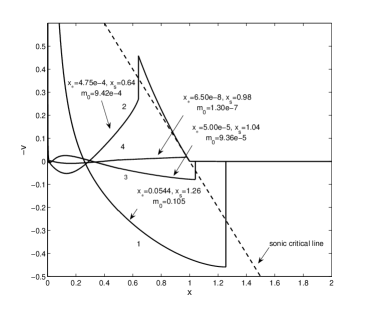
Figure 5: Negative reduced radial speed $-v(x)$ versus $x$ for the four shock solutions identified in the $\alpha-v$ phase diagram of Fig. 4. The straight dashed line is the sonic critical line. Numerals 1, 3, 4, 2 marked along the four solid curves indicate the number of stagnation points corresponding to the shock solutions obtained in Fig. 4 from right to left. Key parameters are shown in the plot. All these shock solutions diverge, approaching $-\infty$ as $x\rightarrow 0^{+}$; such diverging behaviours are displayed more explicitly in Fig. 6 below with the $x-$axis in the logarithmic scale.

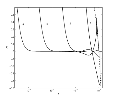
Figure 6: Enlarged portions of Class I shock solution curves near $x\rightarrow 0^{+}$ of Fig. 5, emphasizing the diverging and oscillatory behaviours of this family of shock solutions as $x\rightarrow 0^{+}$. The $x-$axis is shown in the logarithmic scale. The dashed line on the right is the sonic critical line. The undulatory profiles of the curves marked by numerals 2, 3, 4 represent self-similar subsonic radial oscillations with two, three, four stagnation points, respectively.

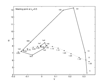
Figure 7: The phase diagram of $\alpha$ versus $v$ at a chosen meeting point $x_{\rm F}=0.5$. Each open circle symbol indicates an integration from $x\rightarrow 0^{+}$ [e.g., $x=10^{-5}$ to start solution (11)] with the central reduced mass density $B$ shown explicitly and each asterisk symbol indicates an integration from the shock location $x_{s}$ with its value marked explicitly. The solid and dotted curves intersect; the first four intersections, from right to left, correspond to the parameter pair {$B$, $x_{s}$} as {7.90, 1.335}, {$9.50\times 10^{4}$, 1.04}, {$1.10\times 10^{7}$, 0.966} and {930, 0.633}, respectively. The variation trend of the phase curves suggest an infinite number of discrete Class II shock solutions matched with a static SIS envelope $A=2$.

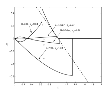
Figure 8: Negative reduced speed $-v(x)$ versus $x$ of the four shock solutions for the four intersections in the $\alpha-v$ phase diagram in Fig. 7. The straight dashed line is the sonic line. Numerals 0, 2, 3, 1 along the four solid curves denote the number of stagnation points in the four shock solutions determined in Fig. 7 from right to left. Downstream portions are LP-type solutions. Key parameters are shown in the plot.

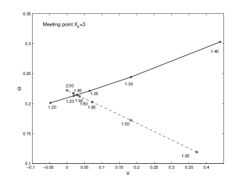
Figure 9: The phase diagram of $v$ and $\alpha$ at a chosen meeting point $x_{\rm F}=3$ for the shock solution with $x_{\ast}=0.5$. Each asterisk symbol indicates an integration from $x_{s}$ with its value shown explicitly and each open circle denotes an integration from $x\rightarrow+\infty$ (actually from $x=20$) with the mass density parameter $A$ also marked explicitly. From the intersection of the solid and dashed curves, we immediately determine the shock location $x_{s}$ and the mass density parameter $A$ for this shock solution.

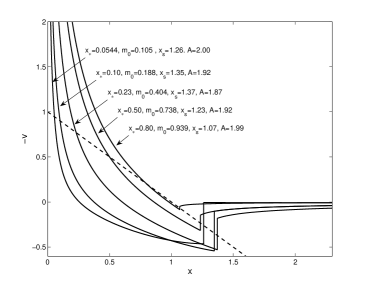
Figure 10: The Class I similarity shock solutions with $V=0$. With one stagnation point, there is only one solution matched with a static SIS envelope. For different $x_{\ast}$, from left to right, the solid curves represent solutions of $x_{\ast}=0.0544,\ 0.10,\ 0.23,\ 0.50,\ 0.80$. Note that the shock locations $x_{s}$ do not vary regularly by shifting $x_{\ast}$. Details of this class of solutions are summarized in Table 2.

In Tsai & Hsu (1995) and Shu et al. (2002), two classes of solutions were derived to match with the static SIS envelope with $V=0$ and $A=2$ or $A<2$. Here, we further explore Class I and Class II solutions matched with the static SIS envelope by searching possible solutions in the phase diagram of $v$ and $\alpha$. This procedure, routinely tested earlier, was first introduced by Hunter (1977; see Lou & Shen 2004 for the EECC solutions). The main technical difference is that in the prior analyses the adjustable parameters are points along the sonic critical line [i.e., horizontal coordinates $x_{\ast}(1)$ and $x_{\ast}(2)$ as in Lou & Shen (2004)], while in our cases, more parameters are involved including $x_{\ast}(1)$, the shock location $x_{s}$, the mass parameter $A$ and the velocity parameter $V=0$. We take one parameter as fixed and adjust the other two to match solutions in the phase diagram of $v$ and $\alpha$.

We first focus on Class I shock solutions with a static SIS envelope, downstream solutions diverging at the centre, and a mass parameter $A=2$ for upstream solutions. Tsai & Hsu (1995) derived a solution in this case and we will explore more thoroughly the phase diagram of $v$ and $\alpha$ to construct more similarity shock solutions. In Fig. 4, we display the relevant phase diagram of $v$ and $\alpha$ where we choose a meeting point at $x_{\rm F}=0.5$ and integrate from $x_{\ast}$(1) forward with a type 2 eigensolution solution to $x_{\rm F}=0.5$. Meanwhile, we use the shock jump condition to determine the $v_{d}$ and $\alpha_{d}$ as the starting condition to integrate backward from a chosen $x_{s}$ to $x_{\rm F}=0.5$. For $x>x_{s}$, we simply set $v=0$ and $A=2$ for a static SIS envelope. Based on Fig. 4, in addition to the solution of Tsai & Hsu, three more similarity shock solutions belonging to this class can be found and are shown for $-v$ versus $x$ in Fig. 5 (the enlarged versions for small $x$ are shown in logarithmic scale in Fig. 6). The variation trend of spiral path in the phase diagram suggests that as a class, there exists an infinite number of discrete similarity shock solutions that connect inner free-fall collapses to an outer static SIS envelope. Each of such solutions is expected to be uniquely associated with a number of stagnation points. From the intersections of the dotted and solid curves in Fig. 4, we obtain four shock solutions, from right to left, corresponding to the displayed solutions marked by 1, 3, 4, 2 in Figs. 5 and 6; these numerals denote the number of stagnation points, and the relevant parameters {$x_{\ast}(1)$, $x_{s}$} are {0.0554, 1.26}, {$5.00\times 10^{-5},1.04$}, {$6.50\times 10^{-8}$, 0.980} and {$4.75\times 10^{-4}$, 0.640}, respectively. The solution containing only one stagnation point is just the solution first found by Tsai & Hsu (1995). We find three new solutions by exploring the phase diagram of $v$ and $\alpha$. In principle, we can construct more solutions following the sequence with increasing number of stagnation points. Behaviours of these solutions at $x\rightarrow 0^{+}$ are displayed in Fig. 6 with velocity profiles crossing the line $v=0$ at different $x$ values. As the value of $x_{\ast}$ becomes smaller, the number of stagnation points increases accordingly. For example, the shock in the shock solution with two stagnation points is an accretion shock such that both downstream and upstream fluids move towards the centre.

We now turn to the Class II shock solutions that connect downstream LP solutions with a static SIS envelope. Tsai & Hsu (1995) first obtained a solution in this case; we shall demonstrate by examples the existence of more such Class II solutions with increasing number of stagnation points. Fig. 7 is a relevant phase diagram of $v$ and $\alpha$ to identify shock solution matches. Here, we choose again a meeting point at $x_{\rm F}=0.5$ and integrate forward from $x\rightarrow 0^{+}$ (e.g., $x=10^{-5}$) where the analytical asymptotic LP solution (11) is imposed with different values of the central reduced density $B$. Meanwhile, we use the shock jump condition to determine $v_{d}$ and $\alpha_{d}$ as the starting condition to integrate from $x_{s}$ back to $x_{\rm F}=0.5$. For $x>x_{s}$, we simply set $v=0$ and $A=2$. The variation trend of spiral structure in Fig. 7 is qualitatively similar to that in Fig. 4, pointing to a class of infinitely many discrete similarity shock solutions that connect inner LP solutions to an outer static SIS envelope. Based on the phase diagram of Fig. 8, the four intersections of the dotted and solid curves give rise to four Class II shock solutions, from right to left, corresponding to solutions marked by the numerals $0,2,3,1$ in Fig. 8; these numerals represent uniquely the number of stagnation points to identify solutions with corresponding parameters {$B$, $x_{s}$} given by {7.90, 1.34}, {$9.50\times 10^{4}$, 1.04}, {$1.10\times 10^{7}$, 0.966} and {930, 0.633}, respectively; the solution with no stagnation point is just the solution found by Tsai & Hsu (1995). As $x\rightarrow 0^{+}$, the self-similar oscillation behaviours of downstream solutions of these Class II shock solutions are similar to those of Class I shock solutions, and as the central reduced density $B$ becomes larger, the number of stagnation points increases. The main difference is that as $x\rightarrow 0^{+}$, Class II shock solutions remain finite while Class I shock solutions diverge for core collapses.

We now summarize the main results of this section. By numerical exploration and analysis, we derived discrete shock solutions matched with a static SIS envelope of $V=0$ and $A=2$ within the semi-complete space of $0<x<+\infty$ (i.e., for $x>x_{s}$, we set $v=0$ and $A=2$). Given this SIS envelope as the upstream condition, we explore classes of infinite number of discrete solutions for both Class I and Class II solutions whose downstreams are free-fall collapses and LP solutions, respectively. For Class I solutions as $x\rightarrow 0^{+}$, the radial velocity and density profiles have asymptotic diverging behaviours (10), while for Class II solutions as $x\rightarrow 0$, the radial velocity and density profiles have finite asymptotic behaviours (11) characterized by a central reduced density $B$. For comparison, the behaviours $x\rightarrow 0^{+}$ of this family of shock solutions with an outer static SIS envelope are similar to those of EECC solutions, viz., both have subsonic oscillations in a self-similar manner as $x_{\ast}\rightarrow 0^{+}$. For Class I solutions as the value of $x_{\ast}$ decreases, the number of stagnation points where $v=0$ along the $x-$axis increases, while for Class II solutions as the value of reduced density $B$ increases, the number of stagnation points increases. The Class I and Class II shock solutions shown by Tsai & Hsu (1995) which contain only one and no stagnation point along $x-$axis, respectively, are special examples belonging to these two classes of shock solutions.

3.3 Similarity Shock Solutions of Breeze

Table 2: Class I shock solutions with an asymptotic breeze

$x_{\ast}$	$m_{0}$	$A$	$x_{s}$	$v_{d}$	$\alpha_{d}$	$v_{u}$	$\alpha_{u}$
0.0554	0.105	2.00	1.26	0.463	2.00	0	1.26
0.10	0.188	1.92	1.35	0.572	1.72	0.102	1.11
0.23	0.404	1.87	1.37	0.529	1.54	0.181	1.09
0.50	0.738	1.92	1.23	0.315	1.63	0.145	1.38
0.80	0.939	1.99	1.07	0.0841	1.87	0.0496	1.81

Columns 1 through 8 list the values of $x_{\ast}(1)$ where the downstream solution crosses the sonic critical line, the reduced central mass accretion rate $m_{0}$, the mass density parameter $A$ for the upstream solution, the shock location $x_{s}$, the downstream velocity $v_{d}$, the downstream density $\alpha_{d}$, the upstream velocity $v_{u}$ and the upstream density $\alpha_{u}$, respectively.

In this section, we allow mass parameter $A$ to vary (i.e., $A\neq 2$) for a fixed $x_{\ast}$ corresponding to a specific reduced central mass accretion rate $m_{0}$. Parameters $A$ and $x_{s}$ are adjusted to match the upstream and downstream solutions in the phase diagram of $v$ and $\alpha$. We integrate from a fixed $x_{\ast}$ (e.g., $0.5$ as shown in Fig. 9) with a type 2 eigensolution to the shock location $x_{s}$ and get the $v_{d}$ and $\alpha_{d}$. Across the shock, we get $v_{u}$ and $\alpha_{u}$ as the starting condition to integrate forward to a chosen meeting point $x_{\rm F}=3$; meanwhile, we integrate back from upstream $x\rightarrow+\infty$ by varying the mass parameter $A$ with a fixed speed parameter $V=0$.

Here, we apply the analytical asymptotic solution (i) as given by equation (9) at $x=20$ as the starting condition to integrate back to $x_{\rm F}$=3. In Fig. 9, we take $x_{\ast}=0.5$ as an example to illustrate the procedure of determining the shock location and the mass parameter $A$ for the upstream solution in the phase diagram of $v$ and $\alpha$. By doing so, we derive a new family of Class I shock solutions. For example, we pick values of $x_{\ast}$ as 0.0544, 0.1, 0.23, 0.5 and 0.8, corresponding to values of $m_{0}=0.105,$ 0.188, 0.404, 0.738, and 0.939, respectively. We find that for Class I shock solutions the value of shock velocity and strength and the mass parameter $A$ do not vary with $x_{\ast}$ regularly as do those for Class II shock solutions. Class I shock solutions with different $x_{\ast}$ are shown in terms of $-v$ and $x$ in Fig. 10; in Table 2, we summarize these solution results. For example, the downstream solutions with $x_{\ast}$=0.1 and 0.5 can match with the upstream solutions for the same mass parameter $A$.

To sum up, we present in this section the similarity solutions with asymptotic breezes, for which, we derived a series of Class I solutions with different central mass accretion rate $m_{0}$ corresponding to different values of $x_{\ast}$. This class of solutions can be applied to processes of cloud collapse in star formation. One important feature of these solutions is that the value of $m_{0}$ is adjustable within the range of 0 to 0.975 corresponding to different central mass accretion rates or shock locations. In one aspect, this family of solutions is analogous to the Class II shock solutions obtained by Shu et al. (2002), i.e., both the upstream solutions are breeze solutions. Two major differences are: (1) our solutions are Class I shock solutions with central free-fall collapses (i.e., diverging solutions as $x\rightarrow 0^{+}$), while the downstream solutions of Shu et al. (2002) are LP solutions. (2) The shock location $x_{s}$ and the mass parameter $A$ for upstream solutions vary regularly as the value of reduced central density $B$ decreases. In contrast, there is no obvious trend of regularity for our Class I shock solutions as $x_{\ast}$ decreases.

3.4 Self-Similar Twin Shock Solutions

Table 3: Class I and II twin shock solutions for different $x_{\ast}(2)$

$x_{\ast}(2)$	Description	$x_{s}(1)$	$x_{s}(2)$	$A$	$V$
0.80	$x_{\ast}(1)=3.40\times 10^{-4}$	0.670	0.85	1.43	-0.528
	$m_{0}=6.20\times 10^{-4}$
	$B=1300$	0.660	0.90	1.52	-0.430
			1.00	1.77	0.192
			1.07	1.99	0
			1.10	2.12	0.109
			1.15	2.36	0.294
0.90	$x_{\ast}(1)=4.40\times 10^{-4}$	0.640	0.95	1.77	-0.198
	$m_{0}=8.18\times 10^{-4}$
	B=1000	0.627	1.00	1.91	-0.0708
			1.05	2.10	0.0831

Columns 1 through 6 list values of $x_{\ast}(2)$ where the Class I twin shock solutions cross the sonic critical line the second time, the key parameters [$x_{\ast}(1)$ and $m_{0}$ for Class I and $B$ for Class II solutions, respectively], the first shock location $x_{s}(1)$, the second shock location $x_{s}(2)$, the mass density parameter $A$ for the upstream solution and the speed parameter $V$, respectively.

Figure 11: The phase diagram of $\alpha$ versus $v$ at a chosen meeting point $x_{\rm F}=0.5$. Each solid dot denotes an integration from $x_{\ast}(1)$ (its value shown explicitly) with type 2 eigensolution, each cross symbol denotes an integration from $x\rightarrow 0^{+}$ (e.g., $x=10^{-5}$) with the value of the central reduced mass density B shown explicitly, and each open circle and asterisk symbols denote integrations from $x_{\ast}(2)=0.8$ and $x_{\ast}(2)=0.9$ respectively via shock condition to the meeting point $x_{\rm F}=0.5$; numerals indicate the shock location $x_{s}$. From the curve intersections, we determine the Class I and II shock solutions for $x_{\ast}=0.8$ and $0.9$, respectively.

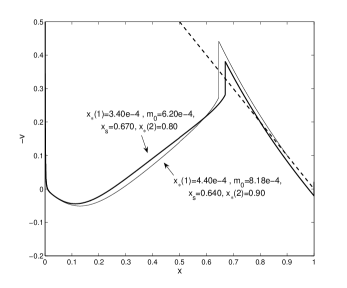
Figure 12: Class I shock solutions with $x_{\ast}(2)=0.8$ and $0.9$ for $-v(x)$ versus $x$ denoted by the light and heavy solid curves, respectively. The straight dashed line is the sonic critical line. The two corresponding values of $x_{\ast}(1)$ are $4.40\times 10^{-4}$ and $3.40\times 10^{-4}$.

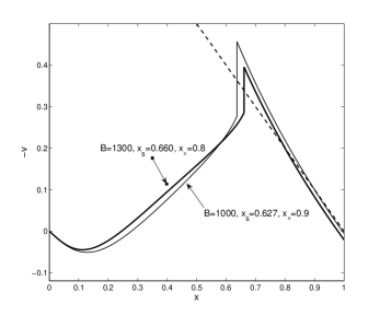
Figure 13: Class II shock solutions with $x_{\ast}=0.8$ and $0.9$ for $-v(x)$ versus $x$ denoted by the light and heavy solid curves, respectively. The straight dashed line is the sonic critical line. Key parameters are shown in the plot.

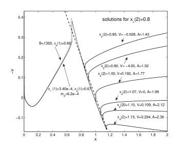
Figure 14: Class I and II twin shock solutions with $x_{\ast}=0.8$ represented by the solid and dotted curves, respectively. The straight dashed line is the sonic critical line. Once the upstream solution of the first shock at $x_{s}(1)$ crosses the sonic critical line analytically at $x_{\ast}=0.8$ with a type 2 eigensolution, we can choose the second shock location $x_{s}(2)=0.85$, 0.90, 1.00, 1.07, 1.10, 1.15 to match with various asymptotic solutions at $x\rightarrow+\infty$.

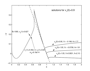
Figure 15: Class I and II twin shock solutions with $x_{\ast}=0.9$ represented by the solid and dotted curves, respectively. The straight dashed line is the sonic critical line. Once the upstream solution of the first shock at $x_{s}(1)$ crosses the sonic critical line analytically, we choose for example $x_{s}(2)=0.95,1.00,1.05$ for the second shock location to match with asymptotic solution at $x\rightarrow+\infty$.

In all previous studies, the similarity shock solutions contain only one shock and the Class I solutions crosses the sonic critical line only once analytically. In this section, we construct similarity shock solutions with twin shocks.

In § 3.2, we find a Class I shock solution crossing the sonic critical line at $x_{\ast}=4.75\times 10^{-4}$ with a shock location $x_{s}=0.640$ and two stagnation points (see Fig. 5), and a Class II shock solution with a central reduced density $B=930$ and a shock location at $x_{s}=0.633$ (Fig. 8) containing only one stagnation point (n.b., the one of $v\rightarrow 0$ as $x\rightarrow 0^{+}$ is not counted here). The portions of upstream solutions between the shock and the static SIS envelope of both shock solutions are tangent to the sonic critical line at the point of $x_{\ast}(2)=1$. In fact, the upstream solution is part of the EWCS (Shu 1977). As we shift the $x_{\ast}(2)$ location leftward into the interval $0<x<1$, the upstream solution of the first (i.e., leftmost) shock may cross the sonic critical line analytically with a type 2 eigensolution. We can then construct Class I and Class II twin shock solutions in the $\alpha-v$ phase diagram given this real possibility.

Let us first focus on Class I twin shock solutions. We fix the value of $x_{\ast}(2)$ and adjust the value of $x_{\ast}(1)$ and the shock location $x_{s}(1)$ between $x_{\ast}(1)$ and $x_{\ast}(2)$ to find the similarity shock solution crossing the sonic critical line twice analytically based on intersections in the $\alpha-v$ phase diagram. On this ground, it is possible to further construct a Class I similarity solution with twin shocks and an appropriate asymptotic solution at $x\rightarrow+\infty$. We take a meeting point at $x_{\rm F}=0.5$ and integrate an upstream solution of the first shock from $x_{\ast}(2)$ for Class I solutions by using a type 2 eigensolution as a starting condition to a chosen shock location $x_{s}(1)$. Based on the velocity and density upstream of this point {$v_{u}$, $\alpha_{u}$}, we use the shock jump conditions (20) and (21) to determine the velocity and density {$v_{d}$, $\alpha_{d}$} downstream of $x_{s}(1)$ and to integrate from $x_{s}(1)$ to $x_{\rm F}=0.5$; meanwhile, we integrate forward from $x_{\ast}(1)$ using another type 2 eigensolution to $x_{\rm F}=0.5$. In Fig. 11, we show the phase diagram for the two cases of $x_{\ast}(2)=0.8$ and $0.9$, respectively. From the intersections of the solid curve and the dotted curve as well as the dashed curve, we obtain the relevant parameter pair {$x_{\ast}(1)$ $x_{s}(1)$} as {$3.40\times 10^{-4}$, 0.670} for the solution with $x_{\ast}(2)=0.8$ and as {$4.40\times 10^{-4}$, 0.640} for the solution with $x_{\ast}(2)=0.9$. We show the corresponding solutions for $-v$ versus $x$ in Fig. 12.

For Class II solutions, we match the upstream and downstream solutions in the $\alpha-v$ phase diagram using a search procedure similar to that of finding the Class I twin shock solutions. Given a fixed $x_{\ast}$, we adjust the value of central reduced mass density $B$ and the shock location $x_{s}(1)$ in order to find matches. At a chosen meeting point $x_{\rm F}=0.5$, we first obtain different parameter sets {$v$, $\alpha$} denoted by cross symbols for different $B$ values by integrating forward from $x\rightarrow 0^{+}$ with the LP solution. We then integrate backward from $x_{\ast}$ to an adjustable shock location $x_{s}(1)$; by imposing the shock condition, we continue to integrate backward towards $x_{\rm F}=0.5$ to obtain a pair of {$v$, $\alpha$}. In Fig. 11, we thus obtain open circle symbols for the case of $x_{\ast}=0.8$ with different $x_{s}(1)$ and asterisk symbols for the case of $x_{\ast}=0.9$ with different $x_{s}(1)$. From the intersections of the dash-dotted curve with the dotted and dashed curves, we find the parameter pair {$B$, $x_{s}(1)$} as {1300, 0.660} and {1000, 0.627} for the shock solutions of $x_{\ast}=0.8$ and $x_{\ast}=0.9$, respectively.

By matching the downstream and upstream solutions in the phase diagram, we obtain the solution structure around the first shock $x_{s}(1)$. For a solution passing the sonic critical line at $x_{\ast}$ the second time, we can further construct the second shock by choosing the different location $x_{s}(2)$ of the second shock. For $x_{\ast}=0.8$, we choose $x_{s}(2)=0.85$, 0.90, 1.00, 1.07, 1.10 and 1.15 while for $x_{\ast}=0.9$, we choose $x_{s}(2)=0.95$, 1.00, 1.05. The upstream solutions across this second shock can match with the analytical asymptotic solution (9) at $x\rightarrow+\infty$; the property of these upstream solutions can evolve from the inflow (contraction or accretion) to outflow (expansion or wind or breeze), as the value of the shock location $x_{s}(2)$ increases.

The main properties of the similarity twin shock solutions are: (1) there exist two stagnation points for the Class I twin shock solutions, while there is only one stagnation point for the Class II twin shock solutions excluding $x\rightarrow 0^{+}$; the spherical stagnation surfaces of zero flow speed travel with different yet constant subsonic speeds, indicating subsonic radial oscillations; (2) the first shock near the core is an accretion shock, as the reduced radial speeds of the pre-shock and post-shock are both negative for inflows. This accretion shock expands at a constant subsonic speed. For the same $x_{\ast}(2)$ and $x_{\ast}$, the velocity of the first shock in Class I solution is a bit larger than that in Class II solution, and for the same class of shock solutions, the velocity of the first shock becomes larger as the $x_{\ast}(2)$ becomes smaller; and (3) the location of the second shock $x_{s}(2)$ can be larger or smaller than 1, such that the velocity of this shock can be supersonic or subsonic. The upstream solution for this shock evolves from the accretion condition to breeze to wind. For different astronomical system, we can construct different shock solutions (e.g., an envelope contraction with core collapse or an envelope expansion with core collapse).

3.5 Two-Temperature Similarity Shock Solutions

Table 4: Class I and II Shock Breeze Solutions with Different $\tau$ Values

Parameters	$\tau$	$A$	$x_{sd}$	$x_{su}$	$v_{d}$	$\alpha_{d}$	$v_{u}$	$\alpha_{u}$
$x_{\ast}(1)=0.23$	1	1.86	1.37	1.37	0.529	1.54	0.181	1.09
	1.3	2.66	1.34	1.74	0.515	1.58	-0.450	0.770
	1.5	3.31	1.31	1.62	0.500	1.62	-0.731	0.732
	1.8	4.49	1.27	2.29	0.480	1.69	-1.12	0.704
$B=0.10$	1	0.23	2.42	2.42	1.76	0.173	0.898	0.0746
	1.3	0.48	2.33	3.03	1.69	0.166	0.575	0.0564
	1.5	0.58	2.29	3.44	1.66	0.164	0.452	0.0521
	1.8	0.78	2.25	4.05	1.62	0.161	0.316	0.0485

Columns 1 to 9 contain shock solution properties [$x_{\ast}(1)$ for Class I solutions and $B$ for Class II solutions]; the ratio $\tau$ of the downstream ($a_{d}$) to upstream ($a_{u}$) sound speed; the mass parameter $A$ for the upstream solution; the downstream shock location $x_{sd}$; the upstream shock location $x_{su}$; the downstream reduced velocity $v_{d}$; the downstream reduced density $\alpha_{d}$; the upstream reduced velocity $v_{u}$ and the upstream reduced density $\alpha_{u}$, respectively.

Table 5: Class II Shock Solutions for $\tau=1.5$ with $B=10^{-6}$.

$x_{sd}$	$x_{su}$	$v_{d}$	$\alpha_{d}$	$v_{u}$	$\alpha_{u}$	$A$	$V$
2.0	3.0	1.44	$1.58\times 10^{-6}$	-0.209	$4.12\times 10^{-7}$	$8.41\times 10^{-7}$	-0.954
3.0	4.5	2.30	$2.73\times 10^{-6}$	1.65	$1.00\times 10^{-6}$	$4.65\times 10^{-6}$	0.998
3.5	5.25	2.76	$3.79\times 10^{-6}$	2.47	$1.51\times 10^{-6}$	$9.61\times 10^{-6}$	1.85

Columns 1 to 8 are the downstream shock location $x_{sd}$; the upstream shock location $x_{su}$; the downstream reduced radial speed $v_{d}$; the downstream reduced density $\alpha_{d}$; the upstream reduced radial speed $v_{u}$; the upstream reduced density $\alpha_{u}$ and the mass parameter $A$ and the speed parameter $V$ for the upstream solution, respectively.

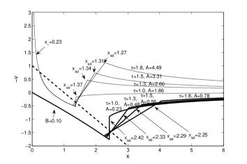
Figure 16: The negative reduced radial speed $-v(x)$ versus $x$ for $\tau\geq 1$. The straight dashed line is the sonic critical line. The light solid curves form the Class I shock breeze or contraction solutions with $x_{\ast}=0.23$ and different $\tau\geq 1$, and the heavy solid curves form the Class II shock breeze solutions with $B=0.10$ for different $\tau\geq 1$. Here, we choose $\tau$ to be 1.0, 1.3, 1.5 and 1.8 to get different shock breeze or contraction solutions.

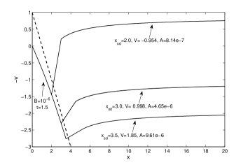
Figure 17: The negative reduced radial speed $-v(x)$ versus $x$. The straight dashed line is the sonic critical line. The solid curves form the Class II shock solutions with $B=10^{-6}$ for $\tau=1.5$. We choose $x_{sd}$ to be 2.0, 3.0, 3.5 to construct different shock solutions matched with asymptotic inflow and winds.

In the preceding sections, we only consider the case of $\tau=1$ corresponding to the same thermal temperature for both downstream and upstream fluids such that the entire fluid has the same sound speed $a_{u}=a_{d}$. For the isothermal condition, the sound speed can be expressed as

$$a=\bigg{(}\frac{P}{\rho}\bigg{)}^{1/2}=\bigg{[}\frac{(Z+1)k}{\mu}T\bigg{]}^{1/2}\ ,$$ (23)

where $k$ is the Boltzmann constant, and sound speed $a$ is determined by the mean atomic mass $\mu$, the ionization state $Z$ and the temperature $T$ together. In some astrophysical processes, these factors determining the sound speed should evolve from an interior region to an exterior region (e.g., HII regions around luminous massive OB stars); in this sense, a fluid may not be treated as an isothermal system. In this section, we will discuss a system of two-temperature fluid. In such a system, the downstream sound speed $a_{d}$ differs from that of the upstream $a_{u}$. Meanwhile, the downstream and upstream fluids can be treated as isothermal fluids respectively. In most astrophysical systems, the downstream sound speed should be larger than that of the upstream. As the central objects heat up the gas around them, we presume $\tau\equiv a_{d}/a_{u}>1$ in our numerical examples.

Let us begin with the shock solutions for the case of $V=0$ at $x\rightarrow+\infty$. Here, we take on Class I solutions with $x_{\ast}(1)=0.23$ and Class II solutions with $B=0.1$ as examples of illustration. By matching the upstream and downstream solutions in the $\alpha-v$ phase diagram at a meeting point $x_{\rm F}$, we obtain the Class I and Class II shock solutions for different values of $\tau$ (e.g., $\tau=10,1.3,1.5,1.8$). In Fig. 16, we display both classes of shock solutions for $-v(x)$ versus $x$. Relevant parameters are summarized in Table 4. For a prescribed boundary condition at $x\rightarrow 0^{+}$ [i.e., $m_{0}$ corresponding to $x_{\ast}(1)$ or the central reduced mass density $B$], as parameter $\tau$ increases, the downstream shock location $x_{sd}$ representing the Mach number of downstream shock becomes smaller; meanwhile, the mass parameter $A$ of the upstream solution increases. For $A<2$, the upstream solution gives an outflow breeze; as the value of $A$ increases, the breeze becomes weaker. For $A>2$, an inward contraction appears at $x\rightarrow+\infty$; the strength of this contraction or inflow becomes larger, as the value of $A$ increases.

We then allow the velocity parameter $V\neq 0$ to vary. As an example, we take $\tau=1.5$ to derive the Class II shock solutions. By choosing different downstream shock locations $x_{sd}$, we construct and display different shock solutions for $-v(x)$ versus $x$ in Fig. 17 with the reduced central density $B=10^{-6}$. Details of such type of two-temperature shock solutions are summarized in Table 5. From this family of shock solutions, we note that with increasing value of $x_{sd}$, the upstream solutions gradually change from an accretion to a wind, and the shock strength becomes weaker. As $x_{sd}$ is increased further, $v_{d}$ will becomes smaller than $v_{u}$ (e.g., $x_{s}=4$ for $\tau=1.5$) which is unphysical. That is, the downstream shock location $x_{sd}$ cannot be arbitrarily large.

4 Astrophysical Applications

Self-similar solutions have been studied to model various astrophysical systems previously (e.g., Larson 1969; Penston 1969; Shu 1977; Tsai & Hsu 1986; Shu et al. 1987, 2002; Lou & Shen 2004; Shen & Lou 2004). There are many instances in which these solutions allow one to develop a numerically simple description of what one first feels is a very complicated astrophysical flow. As results of instabilities and supersonic flows of fluid, accretion and expansion shocks are expected to emerge in various cosmological and astrophysical settings (e.g., supernova explosions; dynamical HII regions surrounding luminous massive OB stars; the dynamic evolution from AGBs to pPNe; accretion shocks around BHs and in quasars; possibly, the creation of initial fireballs in a class of GRBs). In this paper, we mainly focus on various theoretical possibilities and produce different types of similarity shock solutions, including the solutions for a static SIS envelope, for asymptotic breezes or winds or inflows, for twin shocks, for two-temperature fluid and for the global feature of EECC solutions as well as various other possible combinations. Here, we discuss and outline potential astrophysical applications for these similarity shock solutions.

1. The dynamic process connecting the AGB phase and the pPN phase (e.g., Lou & Shen 2004). The stellar evolutionary stage between the end of the AGB phase and the PN phase has long been a key missing link in our physical understanding for the evolution of a single star (e.g., Balick & Frank 2002). A swelling and expanding giant or supergiant star with a massive yet slow wind eventually end up with a more or less detached system containing a small compact and extremely hot white dwarf at its center and a nebula of various morphologies with signatures of shocks indicating interactions of hot faster winds ($\sim 10^{3}\hbox{ km s}^{-1}$) with the massive slow wind ($\sim 10-20\hbox{ km s}^{-1}$). In the gross picture, a dynamic process characterized by self-similar EECC shock solutions may be highly relevant: expansion and outflow of gas materials surrounding a proto-white dwarf in a pPNe, meanwhile infall and collapse in the central core region to produce a compact and hot white dwarf.

Sufficiently far away from initial and boundary conditions, a largely isolated stellar system may gradually evolve into a dynamic phase in a self-similar manner. Available observations suggest the following constraints: (1) the timescale of this collapse-expansion stage is estimated to be $\sim 10^{3}$ yrs; (2) the mass of the central white dwarf should be less than the Chandrasekhar limit of 1.39 M_⊙, otherwise nova-like or even Type Ia supernova-like activities might occur sporadically to produce anomalous abundances in PNe; (3) the massive shell envelope expands with a typical speed of $\sim 10-20$ km s^-1 which is comparable to the sound speed in the gas; (4) there are numerous indications that PNe form involving a much slower wind from the progenitor giant star overtaken by a subsequent faster hot wind presumably generated when a white dwarf emerges, such that shocks are inevitable (Kwok 1978, 1982, 1993; Balick & Frank 2002).

Adopting highly idealized Class I similarity shock solutions constructed in this theoretical analysis, we attempt to provide the following rough estimates in reference to the theoretical central mass accretion rate given by $m_{0}a^{3}/G$ where $a$ is the isothermal sound speed and $G$ is the gravitational constant. Here, we take the sound speed $a$ as $\sim 20$ km s^-1 with a mass accretion rate of the order of $\sim 2m_{0}$ M_⨀/yr. For a timescale of $\sim 10^{3}$ yr, the total accumulated mass onto the central white dwarf would be $\sim 2\times 10^{3}m_{0}$ M_⨀. As the mass limit of a white dwarf $1.39~{}M_{\bigodot}$ and considering the possible range of sound speeds, the parameter $m_{0}$ should fall in the rough range of $\sim 10^{-3}-10^{-4}$. In our analysis, $m_{0}$ associate with the Class I shock solutions with only one stagnation point appears to fit in this range. For example, we may take a Class I twin shock solution with $x_{\ast}(1)=0.8$ with a corresponding $m_{0}=6.20\times 10^{-4}$; this would give a mass of $\sim 1.2$ M_⨀ for the eventual white dwarf. By choosing the second shock location at $x_{s}(2)=1.15$, we can derive the expansion speed of the second shock to be $\sim 20$ km s^-1 and the wind speed of $\sim$6 km s^-1, consistent with observations of wind speed in the range of $\sim 5-10$ km s^-1. We note that there exists an accretion shock in the interior region [i.e., $x_{s}(1)$], which expands at a constant speed of $\sim 13$ km s^-1; this expansive shell form part of interior structures of a PN.

2. Cloud collapses in the star formation process. Shu et al. (1987) reviewed star formation processes in molecular clouds. They suggested to divide the star formation process into four stages. In this scheme, the self-similar evolution may be applicable in relatively early stages referred to as the pre-stellar stage of star formation defined as the dynamic phase in which a gravitationally bound core has formed in a molecular cloud and evolves towards higher degrees of central condensation, but no central hydrostatic protostellar object exists yet (e.g., Andr$\acute{\hbox{e}}$ et al. 1999). As idealization and simplification, a molecular cloud may be treated as spherically symmetric and isothermal during that stage.

With this, the self-similar shock solutions to be used in star formation processes can be classified into two types:

(i) The solutions with an asymptotic radial speed $u\rightarrow 0$ at $r\rightarrow+\infty$. This type of solutions has been discussed by Shu (1977) and Tsai & Hsu (1995) for a static SIS envelope with $V=0$ and $A=2$ in (9). In § 3.3, we derive various breeze solutions with velocity and density profiles and different values of $m_{0}$. For the central mass accretion rate $\dot{M}=m_{0}a^{3}/G$, the value of $m_{0}$ is 0.975 for the EWCS, while in our shock breeze solutions, the range of $0-0.975$ for $m_{0}$ is much wider. This is an important theoretical leeway to account for various central mass accretion rates in protostars. For a typical temperature of 10 K in molecular clouds, we take a sound speed $a=0.2$ km s^-1 and a central mass accretion rate of $\dot{M}\sim 2\times 10^{-6}m_{0}$ M_⨀/yr. As the timescale of this stage is about $10^{6}-10^{7}$ yrs (e.g., Jessop & Ward-Thompson 2001), the formation of a protostar with a mass of $\sim$ 1 M_⨀ would imply a parameter $m_{0}\;\lower 4.0pt\hbox{${\buildrel\displaystyle>\over{\sim}}$}\;0.1$. Meanwhile as the gravitational energy is released during the core collapse, one would expect a point source of infrared luminosity $L_{\rm IR}\sim a^{6}t{m_{0}}^{2}/(GR_{\ast})$ emanating from the dense gas cloud surrounding the core, where $R_{\ast}$ is a protostellar radius taken to be $\sim 3$ R_⨀ (e.g., Stahler 1988). Note that a factor of $m_{0}^{2}$ is involved here. For $m_{0}\sim 1$ as in the case of an EWCS of Shu (1977), this $m_{0}^{2}$ factor is fairly close to $1$. For smaller values of $m_{0}$, this $m_{0}^{2}$ factor may reduce the $L_{\rm IR}$ significantly. For the dense core L1544 in the Taurus molecular complex with a lifetime of $\sim 0.3-0.5$ Myr (e.g., Tafalla et al. 1998) and at the distance of L1544, the sensitivity of the Infrared Astronomy Satellite (IRAS) was about 0.1 L_⨀. As the L1544 cloud system could not be detected by the IRAS, the infrared luminosity $L_{\rm IR}$ should be less than 0.1 L_⨀. From this, we may infer the upper limit of $m_{0}$ to be $\sim 0.1$ for the core of the L1544 cloud system. Among other factors and considerations as well as possibilities, our shock solutions here properly adapted should be applicable to L1544 system. We note that Myers (2005) recently presented the models of free-fall gravitationl collapse in the equilibrium layers, cylinders and Bonnor-Ebert spheres, and the spherical models can match with the observed inward velocity very well. Because of the very little accretion rate of the collapsing Bonner-Ebert sphere in the early stage of the star formation, the model of Bonnor-Ebert spheres may be an alternative way of solving the luminosity puzzle of L1544 cloud system involving centrally condensed collapse of a starless core.

(ii) The shock solutions with a constant asymptotic radial speed $u$ as $r\rightarrow+\infty$. Recent observations have revealed that at sufficiently large distances away from the core, the envelopes of some molecular clouds may expand with a speed of $\sim 0.25$ km s^-1, hinting at the characteristic feature of the EECC shock solutions; these theoretical possibilities were first discussed by Shen & Lou (2004).

3. The ionization and expansion of HII regions. As massive OB stars turn on their central nuclear reactions in modecular clouds, the interstellar medium of surrounding neutral hydrogen gas strongly absorbs the ultraviolet radiation from OB stars and becomes ionized to form HII regions (e.g. Str$\ddot{\hbox{o}}$mgren 1939; Osterbrock 1989 and extensive references therein). As the ionization front sweeps through the cloud, flows driven by pressure gradients develop between HII and HI regions as well as within HII regions, and shocks would conceivably emerge in these processes. Physically similar processes but on much larger scales are also expected to occur in distant quasars and starburst galaxies (e.g., redshifts $z>6$) where surrounding neutral hydrogen gas clouds are irradiated by ultraviolet photons from central accretion or starburst activities and are ionized with subsequent dynamical consequences. For distant quasars, features in the spectral range between the Gunn-Peterson absorption trough (Gunn & Peterson 1965; Scheuer 1965) blueward of the Ly$\alpha$ emission line (e.g., Fan et al. 2001) and the Ly$\alpha$ emission line should contain valuable diagnostic information of the underlying dynamics of HII regions. We shall further pursue this line of research by combining radiative transfer processes with various shock flow models in separate papers. The expansion of the HII regions has been studied for decades (e.g., Newman & Axford 1968; Mathews & O’Dell 1969; Tenorio-Tagle 1979; Franco, Tenorio-Tagle & Bodenheimer 1990; Shu et al. 2002; Shen & Lou 2004). The last two analyses invoked the self-similar shock solutions to model flows and shocks in HII regions. Because of the heating from the central object and the ionization of the gas medium, the sound speed in the inner and outer regions should be different in general. In our relatively simple model framework, a two-temperature fluid separated by a shock may grab certain gross thermal features better. For a given central reduced mass density, by choosing a sound speed ratio of $a_{sd}$ and $a_{su}$ (e.g., $\tau=1.5$) and the shock location $x_{sd}$ ($x_{su}=\tau x_{sd}$), it is possible to construct different shock solutions to match with different asymptotic solutions (e.g., outflow, inflow and static envelope) at $x\rightarrow+\infty$.

We note that when the isothermal approximation is replaced by the polytropic approximation (Suto & Silk 1988; Lou & Gao 2005 in preparation; Wang & Lou 2005 in preparation), it would be more natural to deal with temperature variations in flows and across shocks.

4. Accretion shocks around supermassive black holes such as quasars. Gas materials around quasars fall towards the massive centre following the immense pull of gravity. As the infalling gas with a speed of $\sim 500$ km s^-1 impacts on the core gas materials, a strong accretion shock emerges. Downstream of such a shock, neutral hydrogen gas is expected to be fully ionized. Because of absorptions by the infalling pre-shock gas, a sharp radiative flux drop is observed in quasar spectra indicating the existence of accretion shocks. For the conceptual simplicity, the geometry of such an accretion shock is approximated as spherically symmetric. The temperature of surrounding shock heated gas is higher than $\sim 10^{7}$ K with a sound speed of about several $10^{2}$ km s^-1. Part of the gas is expected to collapse onto the galactic disk eventually. On larger scales, we may apply our similarity shock solutions to model accretion shocks for such a quasar system. In our scenario, the upstream flow velocity is $\sim 0.5$ sound speed corresponding to several $10^{2}$ km s^-1 and the shock front expands at a constant speed of several $10^{2}$ km s^-1. As the lifetime of a quasar is about $10^{8}$ yrs, the radius of such a shock sphere is about 0.1 Mpc and the central mass accretion rate can reach $10^{2}$ M${}_{\bigodot}\hbox{ yr}^{-1}$. This accumulation of materials can assemble the host galaxy of a quasar in a timescale of several $10^{8}$ yrs. These estimates are well consistent with the results of Barkana & Loeb (2003). Generally speaking, in the reservoir of our shock solutions, we could construct other shock solutions that may match with the quasar spectra better. By adjusting locations of the second shock, it is possible to match with various asymptotic envelope solutions.

5. Supernova (SN) explosions and evolution of SN remnants. During the late evolution stage of a massive star, the photodisintegration and the neutronisation of the iron core will reduce the pressure of the inner stellar core, triggering off a rapid core collapse. When the inner core stops collapsing and rebounds the infalling materials, shocks will form and propagate outwards through the inner core, stellar interior and envelope. As the SN envelope expands during the explosion of a SN, it will interact with the circumstellar medium (CSM) and drive another shock through the powerful stellar wind. We note that the speed of SN ejecta could be ultra-relativistic (e.g., Blandford & McKee 1976; Ostriker & McKee 1995; Bisnovatyi-Kogan & Silich 1995) and a gas may be modelled as polytropic (e.g., Goldreich & Weber 1980). In this sense, our isothermal shock solutions may not be directly applicable. However, the relevant concepts and a variety of possibilities shown in this paper are expected to be work for a polytropic gas as well. For example, a shock can not only match with a static envelope but can also match with a wind, as the CSM is contributed to stellar winds in the late evolution stage of a massive star.

By discussions above, we show that similarity shock solutions are potentially applicable to various astrophysical systems, ranging from stellar to galactic scales. There exist collapses, outflows or both collapses and outflows with one or more outward moving shocks in these systems.

5 Summary and Conclusion

In this paper, we explore the self-similar isothermal shock solutions, in reference to the earlier work of Tsai & Hsu (1995), Shu et al. (2002) and Shen & Lou (2004).

First, we have significantly expanded the Class I and Class II shock solutions of Tsai & Hsu (1995) to two families of infinitely many discrete shock solutions matched with a static SIS envelope by systematically searching for intersections in the $\alpha-v$ phase diagram. These shock solutions have subsonic radial oscillations (Shen & Lou 2004). As the value of reduced central mass $m_{0}$ decreases, the number of stagnation points in the corresponding $v(x)$ solution increases. For a given $m_{0}$, the location $x_{\ast}$ of the solution crossing the sonic critical line is fixed. The shock in the solution with two stagnation points is an accretion shock. It is also possible to construct various similarity shock solutions with different values $m_{0}$ to match with asymptotic breeze solutions.

Secondly, we further obtained shock solutions with twin shocks matched with a static SIS envelope. This type of shock solutions contains an inner accretion shock and an outer expansion shock. Both shocks travel outward with constant yet different speeds. The travel speed of the accretion shock is about 0.6 times the sound speed and that of the expansion shock is about the sound speed. By adjusting the outer expansion shock location, twin shock solutions can match with various asymptotic solutions [e.g., inflow (accretion) or outflow (wind)]. We apply this class of shock solutions to bridge the AGB phase and pPN phase. By the property of EECC shock solutions, we suggest to model accretion processes with shocks around black holes.

Finally, by allowing different yet constant temperatures on two sides of a shock (i.e., $\tau>1$ with the downstream temperature higher than the upstream temperature), we derived shock solutions in a two-temperature fluid to match with various asymptotic solutions at $x\rightarrow+\infty$. These shock solutions may describe cloud collapse leading to star formation and expansion of HII regions surrounding massive OB stars.

In our model analysis, we pursue a simple isothermal scenario. This is a special case of the more general polytropic treatment (Cheng 1978; Goldreich & Weber 1980; Yahil 1983; Bouquet et al. 1985; Suto & Silk 1988; Maeda et al. 2002; Harada et al. 2003; Fatuzzo et al. 2004; Wang & Lou 2005 in preparation). Shock solutions have also been derived in the polytropic case (Lou & Gao 2005, in preparation). Polytropic shock solutions should have an even wider range of astrophysical applications.

Appendix A Solution Matching

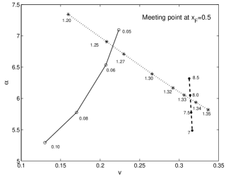
Figure 18: The phase diagram of $v$ versus $\alpha$ at the meeting point $x_{\rm F}=0.5$. Each asterisk symbol denotes an integration back from the shock location $x_{s}$ with its value shown explicitly; each solid dot denotes an integration from $x\rightarrow 0^{+}$ for an inner LP solution [equation (11)] with the parameter $B$ marked explicitly; each open circle denotes an integration from $x_{\ast}$ with its value shown explicitly and this integration starts from a type 2 eigensolution across the sonic critical line $x-v=1$. For Class I shock solution, we determine the location $x_{\ast}=0.0544$ where the flow solution crosses the sonic critical line analytically and the shock location $x_{s}=1.26$ from the intersection point of the solid and dotted curves in the $v-\alpha$ phase diagram. For Class II shock solution, we deterimine the reduced core density $B=7.9$ and the shock location at $x_{s}=1.34$ from the intersection point of the dashed and dotted curves.

We determine the parameters $x_{\ast}$, $x_{s}$ and $B$ by continuously varying relevant parameters to search for intersections of the two curves $v$ and $\alpha$ in the phase diagram of $v$ versus $\alpha$ where the meeting point is taken to be $x_{\rm F}=0.5$. We integrate nonlinear ODEs (7) and (8) from $x_{\ast}\ (<x_{\rm F})$ by using the type 2 eigensolutions across the sonic critical line as specified by equation (13) to $x_{\rm F}=0.5$ for Class I solutions or independently, from $x\rightarrow 0^{+}$ by using the LP-type solution specified by (11) as the starting condition to $x_{\rm F}=0.5$ for Class II solutions. In this manner, we obtain a pair of $v$ and $\alpha$ in the so-called phase diagram. By gradually varying parameter $x_{\ast}$ (for Class I) or $B$ (Class II), the values of $v$ and $\alpha$ at the meeting point $x_{\rm F}$ will change continuously in the $v-\alpha$ phase diagram. In Fig. 18, we show such phase curves in solid and dashed curves for Classes I and II solutions, respectively.

Meanwhile, we choose different shock locations and apply the jump condition (20) to obtain compatible $v_{d}$ and $\alpha_{d}$ as the starting condition and integrate back from $x_{s}$ to $x_{\rm F}=0.5$ to determine values of $v$ and $\alpha$ at $x_{\rm F}=0.5$; the dotted curve in Fig. 18 is obtained this way and from the intersections between the dotted curve and the solid and dashed curves, we determine parameters $x_{\ast}$, $x_{s}$ and $B$ for relevant similarity shock solutions.

The mass parameter $A$ and shock location $x_{s}$ for the shock solution of Shu et al. (2002) for a given $B$ can be determined from the phase diagram of $v$ versus $\alpha$. Two specific examples are shown in Fig. 19 for $B=1$ and $B=4$, with the meeting point chosen at $x_{\rm F}=3$. The numerical procedure is similar to that described in § 3.1.1.

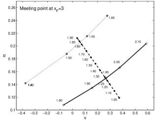
Figure 19: The phase diagram of $v$ versus $\alpha$ at the meeting point $x_{\rm F}=3$. Each asterisk symbol indicates an integration from the shock location $x_{s}$ with its value shown explicitly for $B=4$; each open circle symbol indicates an integration from the shock location $x_{s}$ with its value shown explicitly for the case of $B=1$; each solid dot denotes an integration from $x\rightarrow+\infty$ (practically, we take $x=20$) to use the analytical asymptotic solutions (9) with the velocity parameter $V=0$ and the mass density parameter $A$ with its value marked explicitly. From the intersections of the dashed curve with the dotted curve and the solid curve, respectively, we determine the shock location $x_{s}$ and the value of mass density parameter $A$ for $B=4$ and $B=1$, respectively.

References

- \beginrefs
- [1] Andr P., Ward-Thompson D., Barsony M., 1999, in Protostars & Planets IV, eds. V. Mannings, A. Boss, S. Russell (Tucson: The University of Arizona Press), astro-ph/993284
- [2] Balick B., Frank A., 2002, ARA&A, 40, 439
- [3] Barkana R., Leob A., 2003, Nature, 421, 341
- [4] Blandford R. D., McKee C. F., 1976, Phys. Fluids, 19, 1130
- [5] Bisnovatyi-Kogan G. S., Silich S. A., 1995, Rev. Mod. Phys., 67, 661
- [6] Bouquet S., Feix M. R., Fijakow E., Munier A., 1985, ApJ, 293, 494
- [7] Boily C. M., Lynden-Bell D., 1995, MNRAS, 276, 133
- [8] Cheng A. F., 1978, ApJ, 221, 320
- [9] Courant R., Friedrichs K. O., 1976, Supersonic Flow and Shock Waves. Springer-Verlag, New York
- [10] Fan X., et al. 2001, AJ, 122, 2833
- [11] Fatuzzo M., Adams F. C., Myers P. C., 2004, ApJ, 615, 813
- [12] Franco, J., Tenorio-Tagle, G., Bodenheimer, P. 1990, ApJ, 349, 126
- [13] Gunn J. E., Peterson B. A., 1965, ApJ, 142, 1633
- [14] Goldreich P., Weber S. V., 1980, ApJ, 238, 991
- [15] Harada T., Maeda H., Semelin B., 2003, Phys. Rev. D, 67, 084003
- [16] Hunter C., 1977, ApJ, 218, 834
- [17] Hunter C., 1986, MNRAS, 223, 391
- [18] Jessop N. E., Ward-Thompson, D., 2000, MNRAS, 311, 63
- [19] Kwok S., 1978, ApJ, 219, L125
- [20] Kwok S., 1982, ApJ, 258, 280
- [21] Kwok S., 1993, ARA&A, 31, 63
- [22] Larson R. B., 1967a, MNRAS, 145, 271
- [23] Larson R. B., 1967b, MNRAS, 145, 405
- [24] Landau L. D., Lifshitz E, M., 1959, Fluid Mechanics, Pergamon Press, New York
- [25] Lazarus R. B., 1981, SIAM, J. Numer. Anal., 18, 316
- [26] Lou Y. Q., Shen Y., 2004, MNRAS, 348, 717 (astro-ph/0311270)
- [27] Lou Y. Q., Gao Y., 2005, MNRAS, in preparation
- [28] Maeda H., Harada T., Iguchi H., Okuyama N., 2002, Progress of Theoretical Physics, 108, 819
- [29] Mathews W. G., O’Dell, C. R., 1969, ARA&A, 7, 67
- [30] Myers, P. C., 2005, ApJ, 623, 280
- [31] Murakami M, Nishihara K, Hanawa T, 2004, ApJ, 607, 879
- [32] Newman R. C., Axford W. I., 1968. ApJ, 153, 595
- [33] Osterbrock D. E., 1989, Astrophysics of Gaseous Nebulae and Active Galactic Nuclei, Mill Valley, Calif.
- [34] Ostriker J. P., McKee C. F., 1988, Rev. Mod. Phys., 61, 1
- [35] Penston M. V., 1969a, MNRAS, 144, 425
- [36] Penston M. V., 1969b, MNRAS, 145, 457
- [\citeauthoryearPress et al.1986] Press W. H., Flannery B. P., Teukolsky S. A., Vetterling W., 1986, Numerical Recipes (Cambridge: Cambridge Univ. Press)
- [37] Scheuer P., 1965, Nature, 207, 963
- [38] Shen Y., Lou, Y. Q., 2004 ApJ 611 L117 (astro-ph/0407328)
- [39] Shen Y., Lou, Y. Q., 2005 ChJAA 5, 38 (astro-ph/0410051)
- [40] Stahler S. W., 1988, ApJ, 332, 804
- [41] Sedov L. I., 1959, Similarity and Dimensional Methods in Mechanics. Academic, New York
- [42] Shu F. H., 1977, ApJ, 214, 488
- [43] Shu F. H., Adams F. C., Lizano S., 1987, ARA&A, 25, 23
- [44] Shu F. H., Lizano S., Galli D., Cant J., Laughlin G., 2002 ApJ, 580, 969
- [45] Spitzer L., Physical Process in the Interstellar. Wiley. N. Y.
- [46] Strmgren B., 1939, ApJ, 89, 526
- [47] Suto Y., Silk J., 1988, ApJ, 326, 527
- [48] Tafalla M., Mardones D., Myers P. C., Caselli P., Bachiller R., Benson, P. J., 1998, ApJ, 504, 900
- [49] Tenorio-Tagle, G. 1979, A&A, 71, 59
- [50] Tsai J. C., Hsu J. J. L., 1995, ApJ, 448, 774
- [51] Yahil A., 1983, ApJ, 265, 1047
- [52] Yu C., Lou Y.-Q., 2005, MNRAS, submitted