Approximate Consistency Condition from Running Spectral Index in Slow-Roll Inflationary Models

Abstract

Density perturbations generated from inflation almost always have a spectral index $n_{s}$ which runs (varies with the wavelength). We explore a running spectral index scenario in which the scalar spectral index runs from blue ($n_{s}>1$) on large length scales to red ($n_{s}<1$) on short length scales. Specifically, we look for a correlation between the length scale at which $n_{s}-1=0$ and the length scale at which tensor to scalar ratio $\mathcal{T}/\mathcal{S}$ reaches a minimum for single field slow roll inflationary models. By computing the distribution of length scale ratios, we conclude that there indeed is a new approximate consistency condition that is characteristic of running spectral index scenarios that run from blue to red. Specifically, with strong running, we expect 96% of the slow roll models to have the two length scales to be within a factor of 2, with the length scale at which the tensor to scalar ratio reaching a minimum longer than the wavelength at which $n_{s}-1=0$.

I Introduction.

It is currently widely accepted that inflationary cosmological scenarios offer most promising explanations for the initial conditions for structure formation in our universe. Almost all inflationary scenarios predict that the primordial density perturbation spectrum deviates slightly from a power law and is dominated by scalar density fluctuations. Typically, the scalar density perturbation spectrum is parameterized as

$$P_{S}(k)=A_{S}^{2}(\frac{k}{k_{*}})^{n_{s}(k)-1}$$ (1)

where $n_{s}(k)\approx 1$ is a scale dependent function which is usually called the running (scalar) spectral index (running refers to the change in the spectral index as a function of wavenumber $k$). Combining observations of CMB, galaxy surveys, and Ly$\alpha$ forest, there have been claims for evidence of strongly running spectral index (see e.g. Peiris:2003ff ), but at the moment, combined data set favors no spectral index running (e.g. Seljak:2004xh ). Nonetheless, a significant running of the spectral index is still a debatable possibility that will be settled by future experiments.

According to the CMB and 2dFGRS galaxy survey data Bennett:2003bz ; Percival:2001hw ,

$$\frac{dn_{s}}{d\ln k}(k=0.05\mbox{Mpc}^{-1})=-0.03^{+0.016}_{-0.018}\ .$$ (2)

Furthermore, as pointed out by Peiris:2003ff , within the context of single field inflationary models, there is some indication that the spectral index quantity $n_{s}-1$ runs from positive values (blue) on long length scales to negative values (red) on short length scales (positive to negative within about 5 e-folds).

It is well known Lidsey:1995np that one robust check of slow roll inflationary scenario is what is usually referred to as the single field self-consistency condition

$$n_{T}(k)=-2\epsilon$$ (3)

where $n_{T}$ is the spectral index of tensor perturbation power spectrum parameterized as $P_{T}\propto k^{n_{T}}$ and $\epsilon$ is the slow roll parameter characterizing the tensor to scalar power spectrum ratio. In Chung:2003iu , it was pointed out that if running occurs from blue to red, then there may be another approximate consistency condition that we may observationally aim at checking regarding inflationary scenarios. Namely, within the single field slow roll scenario, there should be an approximate coincidence between the length scale $k_{1}$ at which

$$n_{s}(k_{1})-1=0$$ (4)

and the length scale $k_{2}$ at which the tensor to scalar ratio reaches a minimum, i.e.

$$\epsilon^{\prime}(k_{2})=0.$$ (5)

If true, this kind of new consistency condition would be important because currently there is only a very limited number of observational consistency checks that could support the picture of inflationary origin of density perturbations.

The degree to which

$$k_{1}\approx k_{2}$$ (6)

depends on a) how fast $n_{s}(k)$ runs and b) the slow roll parameter $\epsilon$ (this is true at least in the leading slow roll order approximation). Hence, it is not clear how compelling the expectation of this coincidence is. For example, does Eq. (6) occur only for 1 out of 10,000 slow roll models of inflation with running spectral index or does it occur for 9000 out of 10,000 slow roll models of inflation? Furthermore, because of the strongly running behavior of the spectral index, it was not clear that the leading order presented in Chung:2003iu was robust. Hence, in this paper, we quantify the degree to which one would find the approximate consistency condition a compelling consistency check of single field inflationary scenario. Furthermore, we check that the qualitative expectation based on first order slow roll expansion is also valid at second order slow roll expansion.

In the spirit of Kinney:2003uw , we examine a grid of slow roll models and ask how the distribution of $k_{1}/k_{2}$ changes as a function of increasing the requirement of running spectral index. Expressed in terms of difference in the e-folds of inflation (expressed as $k_{1}/k_{2}=\exp(\Delta N)$), we find $\Delta N$ has a mean of about $-0.34$ with a $2\sigma$ width of $0.5$ when a strong running condition is imposed as when both $0.15<n(k=0.002\mbox{Mpc}^{-1})-1<0.3$ and $-0.3<n(k=1\mbox{Mpc}^{-1})<-0.15$ are satisfied. Hence, slow roll inflationary scenarios predict that there should be a coincidence of $k_{1}$ and $k_{2}$ within a factor of two if the spectrum runs from blue to red, and the mismatch is such that $k_{1}>k_{2}$. Furthermore, since the $2\sigma$ width of the distribution without strong running condition is about $1.2$, we find quantitative evidence that if the spectral index runs strongly, there is an increase in the coincidence as expected.

There are two main caveats to our results. As discussed in Section IV, because the B-mode polarization sensitive to tensor perturbations is expected to peak on relatively large angular scales where it is measurable with current forecasts Knox:2002pe ; Cooray:2005xr while the minimum of tensor to scalar ratio lies on shorter angular scales, measurements testing the proposed approximate consistency condition may be difficult. If strong running is relevant to cosmology, ingenuity of scientists in the future will hopefully overcome this obstacle. The second is that the grid of models that we choose are sampled with equal weight for the initial conditions of the slow roll equation. Although this is commonly found in the literature Peiris:2003ff ; Kinney:2003uw ; Dodelson:1997hr ; Boyle:2005ug and does not seem to be an unreasonable way to sample the possible set of models, this kind of probability measure does not have any justification from first principles. A similar ambiguity of measure plagues most “landscape” or anthropic principle arguments (e.g. Banks:2003es ).

This paper is organized as follows. In the next section, we analytically compute the coincidence in terms of slow roll parameters. Following that we present numerical results. Measurement prospects are then discussed in Section IV. In the appendix, we collect some useful slow roll formulas used in the derivations in the paper. Throughout this paper, we use the convention $M_{p}=1/\sqrt{G_{N}}$.

II Analytical approximation

Let us see why there should be an approximate consistency condition as described in the introduction. In Chung:2003iu , it was shown that within the context of a single real scalar field $\phi$ slow roll inflationary model with a potential $V(\phi)$, one can write

$$\frac{n_{s}-1}{\sqrt{2\epsilon_{V}}}+\sqrt{2\epsilon_{V}}=\pm\frac{\epsilon_{V}^{\prime}(\phi)}{\epsilon_{V}(\phi)}$$ (7)

where $\epsilon_{V}\equiv\frac{M_{p}^{2}}{16\pi}(V^{\prime}/V)^{2}$ is the usual inflationary slow roll parameter in terms of the potential, the upper (lower) sign is for $V^{\prime}(\phi)>0$ ($V^{\prime}(\phi)<0$). Since the tensor to scalar ratio is given by $P_{g}/P_{\mathcal{R}}=16\epsilon_{V}$, the vanishing of the right hand side of Eq. (7) corresponds to the scale at which the tensor to scalar power reaches an extremum. Now, the observation that was made was that if the spectrum runs from blue to red, then $\pm\epsilon_{V}^{\prime}$ will be positive initially, but as $n_{s}-1$ becomes negative to the point of canceling the $2\epsilon_{V}$, $\epsilon_{V}^{\prime}$ will vanish. As long as $\epsilon_{V}$ is small and/or $n_{s}-1$ runs strongly negative, the scale at which $n_{s}-1$ crosses zero will coincide with the extremum of $\epsilon_{V}$ which in turn corresponds to the extremum of the tensor to scalar ratio.

In this section we will extend the previous derivation to second order in slow roll and confirm the qualitative validity of the previous results. This is reassuring given that the validity of leading order results was questionable in light of strongly running behavior. To accomplish this task, we will work with Hubble flow slow roll expansion techniques (see, e.g. Lidsey:1995np ). The advantage of the Hubble flow approach is that it is simpler to go to higher orders in derivative expansion.

Using the conventions of liddle94 , we use the definitions for the slow roll parameters in terms of the Hubble function $H\left(\phi\right)$ as follows:

$$\epsilon \equiv {M_{p}^{2}\over 4\pi}\left({H^{\prime}(\phi)\over H(\phi)}\right)^{2}$$ (8)

$$\eta\left(\phi\right) \equiv {M_{p}^{2}\over 4\pi}\left({H^{\prime\prime}\left(\phi\right)\over H\left(\phi\right)}\right)$$ (9)

$$\sigma \equiv {M_{p}^{2}\over\pi}\left[{1\over 2}\left({H^{\prime\prime}\over H}\right)-\left({H^{\prime}\over H}\right)^{2}\right]$$ (10)

$${}^{\ell}\lambda_{\rm H} \equiv \left({M_{p}^{2}\over 4\pi}\right)^{\ell}{\left(H^{\prime}\right)^{\ell-1}\over H^{\ell}}{d^{(\ell+1)}H\over d\phi^{(\ell+1)}}.$$ (11)

Here, the Hubble function is defined by the Hamilton-Jacobi equations

$$\dot{\phi} = -\frac{M_{p}^{2}}{4\pi}\frac{dH}{d\phi}$$ (12)

$$\left(\frac{dH}{d\phi}\right)^{2}-\frac{12\pi}{M_{p}^{2}}H^{2} = \frac{-32\pi^{2}}{M_{p}^{4}}V(\phi)$$ (13)

which has the advantage of having a readily solvable model of power law inflation. As is well known, Hubble flow slow roll expansion that we summarize below is a derivative expansion in $H(\phi)$ about the power law inflationary model.

We used $N$ as the measure of time during inflation, the number of e-folds before the end of inflation, which increases as one goes backward in time :

$${d\over dN}={d\over d\ln a}={M_{p}\over 2\sqrt{\pi}}\sqrt{\epsilon}{d\over d\phi},$$ (14)

with the sign convention

$$\sqrt{\epsilon}\equiv+{m_{\rm p}\over 2\sqrt{\pi}}{H^{\prime}\over H}.$$ (15)

These equations implies a relationship of $\epsilon$ to $H$ and $N$:

$${1\over H}{dH\over dN}=\epsilon.$$ (16)

The evolution of the higher order parameters during inflation is determined by a set of “flow” equations hoffman00 ; schwarz01 ; kinney02 ,

$${d\epsilon\over dN} = \epsilon\left(\sigma+2\epsilon\right),$$ (17)

$${d\sigma\over dN} = -5\epsilon\sigma-12\epsilon^{2}+2\left({}^{2}\lambda_{\rm H}\right),$$ (18)

$${d\left({}^{\ell}\lambda_{\rm H}\right)\over dN} = \left[\frac{\ell-1}{2}\sigma+\left(\ell-2\right)\epsilon\right]\left({}^{\ell}\lambda_{\rm H}\right)+{}^{\ell+1}\lambda_{\rm H}.$$ (19)

As one can see, in general any slow roll parameter could be expressed in terms of one single slow roll and its derivatives. Some of these relationships are explicitly given in the appendix. Note that $\epsilon$ has the interpretation through the fact that tensor to scalar power spectrum is given by

$$\frac{P_{g}}{P_{\mathcal{R}}}=16\epsilon$$ (20)

where $P_{g}$ and $P_{\mathcal{R}}$ are the usual power spectrum for tensor and scalar gauge invariant metric perturbations.

Let us now solve for the difference between the length scale at which $\epsilon$ reaches an extremum ($1/k_{2}$) and the length scale at which $n_{s}-1$ crosses 0 ($1/k_{1}$). Instead of giving the length scale in terms of the inverse wave vector, we will express it terms of the difference in the horizon exit e-folds $\Delta N$. To translate that into ratio of lengths, one simply has

$$\ln(\frac{k_{2}}{k_{1}})=\Delta N=N_{1}-N_{2}+\mathcal{O}(\ln(H_{2}/H_{1}))$$ (21)

where $H_{2}$ is the expansion rate when $k_{2}$ left the horizon and $H_{1}$ is the expansion rate when $k_{1}$ left the horizon. Since $\ln(H_{2}/H_{1})$ is of order of the slow roll parameter during the early stages of inflation, one can disregard this term when interpreting $\Delta N\equiv N_{1}-N_{2}$ as long as it is larger than about $0.1$. Defining $N_{0}$ as the point where the extremum of $\epsilon$ occurs, i.e. $\frac{d\epsilon}{dN}|_{N_{0}}=0$, we can linearize $n_{s}-1$ around it to solve approximately for $\Delta N$. Using the formulas given in the appendix, we can write

$$n_{s}(N_{0}+\Delta N)-1\simeq n_{s}(N_{0})-1+\frac{dn_{s}}{dN}|_{N_{0}}\Delta N$$ (22)

$$\frac{dn_{s}}{dN}=-\frac{2\epsilon^{2}\dot{\epsilon}-\dot{\epsilon}^{2}-\epsilon\ddot{\epsilon}}{\epsilon^{2}}$$ (23)

$$n_{s}-1=\frac{1}{4\epsilon^{2}}\{(-3+C)\dot{\epsilon}^{2}+\left[4\epsilon+2\epsilon^{2}(C+3)\right]\dot{\epsilon}+\ddot{\epsilon}(3-C)-8\epsilon^{3}(\epsilon+1)\}.$$ (24)

Solving $n_{s}(N_{0}+\Delta N)-1=0$ for $\Delta N$, we obtain

$$\Delta N_{analytical}\approx\frac{C-3}{4}+\frac{2\epsilon(1+\epsilon)}{\frac{dn_{s}}{dN}(N_{0})}.$$ (25)

The constant $C\equiv 4(\ln{2}+\gamma)-5=0.0814514$, where $\gamma\simeq 0.577$ is Euler’s constant. As it can be seen from this formula $\Delta N$ clusters around the negative value $-0.67$ and it can be positive or negative. We can also observe that stronger running (associated with a higher slope for $n_{s}$) drifts $\Delta N$ toward more negative values, and that this effect is modulated by the value of $\epsilon$ at $N_{0}$.

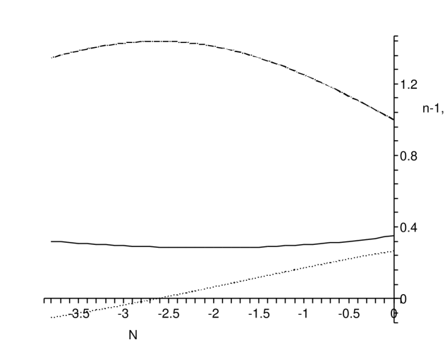
Figure 1: From the graph of $\epsilon$ , $P_{\mathcal{R}}$ (scalar power spectrum), and $n_{s}-1$ as functions of the number of e-folds $N$, it can be seen that the extrema of $\epsilon$ and $P_{\mathcal{R}}$ are closed to the point where $n_{s}-1$ is zero. The dot dashed curve is $P_{\mathcal{R}}/P_{\mathcal{R}}(0)$, the solid curve is $50\epsilon$, and the dotted curve is $n_{s}-1$. The horizontal axis is oriented such that inflation ends at $N<-3.5$ (i.e. time flows right to left).

We will see that numerical results agree well with the analytical approximation. Before going onto numerical analysis, we would like to note that beyond Eq. (7), there may be many more “approximate consistency” conditions associated with strong running since we are merely labeling various features of the slow roll equations. For example, as it can be inferred already from the first order formula $P_{k}^{\zeta}=\frac{8V_{k}}{3\epsilon M_{p}^{4}}$ the power spectrum will have an extremum roughly coinciding with the extrememum of $\epsilon$ . To check this numerically, we can examine an example of an inflationary model (as explained in the next section). As it can be seen in Fig. 1, the scalar power spectrum has an extremum very closed to the point where $n_{s}-1$ is zero. We could proceed similarly to the way we have done for Eq. (6), comparing analytical approximation to numerical data for this “approximate consistency” condition, which in this case would not depend on the strength of the running of the spectral index, but could be another test for more general inflation models.

III Numerical approach

In this section, we study our proposed approximate consistency condition question numerically. One scientific question we would like to address is, “What is the expected coincidence of the value $k_{1}$ satisfying $n_{s}(k_{1})-1=0$ with the value $k_{2}$ satisfying $\epsilon^{\prime}(\phi_{k_{2}})=0$?” The second question is whether a stronger negative running of the spectral index makes the expected $|k_{1}-k_{2}|$ significantly smaller.

To this end, we examine a particular grid (to be specified below) of slow roll inflationary models. In this grid of models, we make a set of “cuts” which select out subsets of the models with scalar spectral index running from blue to red. In this way, we can make a histogram of models as a function $\Delta N$ (defined in Eq. (21)). The peak and the width of the histogram quantifies the expected coincidence of $k_{1}$ with $k_{2}$, answering our first question. We then make the cuts more stringent such that only those slow roll models with more strongly running spectral indices are included in the histogram. The degree to which the width of the histogram changes as we make the required running stronger answers our second question.

Let us now explain the details which closely follows the methods of Kinney:2003uw . Assigning a set of initial conditions to Eqs. (19) and integrating them specifies a flow of the slow roll function. Each of the initial conditions corresponds to a particular choice of inflaton potential and the inflaton initial conditions. We choose initial values for the parameters at random from the following ranges, assuming a uniform probability distribution :

$$N = [40,70]$$ (26)

$$\epsilon = \left[6\ 10^{-76},0.6\right]$$ (27)

$$\sigma = \left[-0.5,0.5\right]$$ (28)

$${}^{2}\lambda_{\rm H} = \left[-0.05,0.05\right]$$ (29)

$${}^{3}\lambda_{\rm H} = \left[-0.025,0.025\right],$$ (30)

$$\cdots$$ (31)

$${}^{M+1}\lambda_{\rm H} = 0.$$ (32)

We truncated the expansion to order 5 by setting ${}^{6}\lambda_{\rm H}=0$. We calculate the values of the tensor/scalar ratio $r$, the spectral index $n$, and the “running” of the spectral index $dn/d\ln k$ according to: liddle94 ; stewart93

$$r=10\epsilon\left[1-C\left(\sigma+2\epsilon\right)\right],$$ (33)

$$n_{s}-1=\sigma-\left(5-3C\right)\epsilon^{2}-{1\over 4}\left(3-5C\right)\sigma\epsilon+{1\over 2}\left(3-C\right)\left({}^{2}\lambda_{\rm H}\right)$$ (34)

Note that the variable $r$ here is defined with a different normalization than in Peiris:2003ff where $r\approx 16\epsilon$ to leading slow-roll order. A comoving scale $k$ crossed the horizon a number of e-folds $N(k)$ before the end of inflation : lidsey97

$$N(k)=62-\ln\frac{k}{a_{0}H_{0}}-\ln\frac{10^{16}{\rm GeV}}{V_{k}^{1/4}}+\ln\frac{V_{k}^{1/4}}{V_{e}^{1/4}}-\frac{1}{3}\ln\frac{{V_{e}}^{1/4}}{\rho_{{\rm RH}}^{1/4}}\,.$$ (35)

Here $V_{k}$ is the potential at horizon exit, $V_{e}$ is the potential at the end of inflation, and $\rho_{{\rm RH}}$ is the energy density after reheating. Note that since slow roll inflation evolves toward decreasing potential, we can write

$$V_{e}=f_{k}^{4}V_{k}$$ (36)

where $f_{k}<1$ is a function of $k$ that varies as to keep $V_{e}$ independent of $k$. Furthermore, since the reheating energy density must be smaller than $V_{e}$, we can write

$$\rho_{{\rm RH}}=\gamma^{4}V_{e}$$ (37)

where the proportionality constant satisfies $\gamma<1$. Using Eq. (35), derivatives with respect to wavenumber $k$ can be expressed in terms of derivatives with respect to $N$ as liddle95

$${d\over dN}=-\left(1-\epsilon\right){d\over d\ln k},$$ (38)

Hence, the running of the spectral index can be expressed to third order in slow roll parameters as

$$\frac{dn_{s}}{d\ln k} = \frac{1}{4(1-\epsilon)}\left[48\,{{\epsilon}}^{2}+\left(44+12\,C\right){{\epsilon}}^{3}+\left(-9\,C+31\right){{\epsilon}}^{2}\sigma+\left(-5\,C+3\right){\epsilon}\,{\sigma}^{2}\right.$$ (39)

$$\left.+\left(-10\,C+6\right)({}^{2}\lambda_{\rm H}){\epsilon}+\left(C-3\right)({}^{2}\lambda_{\rm H})\sigma++20\,{\epsilon}\,\sigma-8\,({}^{2}\lambda_{\rm H})+\left(2\,C-6\right)({}^{3}\lambda_{\rm H})\right]$$

We will now use superscripts a and b to denote quantities evaluated at or corresponding to the length scale $k^{a}=0.002\mbox{ Mpc}^{-1}$ or $k^{b}=1\mbox{ Mpc}^{-1}$. The algorithm for generating the histogram of Fig. 1 can then be described as follows:

1. A set of random initial conditions was generated for the value of the slow roll parameters at $N^{a}$. The following constraints are imposed:

   $$r^{a}<0.5$$ (40)

   $$n^{a}_{l}<n_{s}^{a}-1<n^{a}_{u}$$

   $${\frac{dn_{s}}{d\ln k}}^{a}<0$$

   where $n^{a}_{u}$ is fixed to 0.3 and $n^{a}_{l}$ varies from 0 to 0.225 for different cuts with a 0.075 increment. If these constraints are respected, proceed to step 2 otherwise go back to step 1.

2. Integrate the flow equation (using LSODA from ODEPACK Hindmarsh:1983 ) to $N^{b}$ and then check the following constraints:

   $$n^{b}_{l}<n_{s}^{b}-1<n^{b}_{u}$$

   where $n^{b}_{l}$ is fixed to -0.3 and $n^{b}_{u}$ varies from 0 to -0.225 for different cuts with a 0.075 increment. If these are respected go to step 3 otherwise go to step 1.

3. Evolve forward in time ($dN<0$) until inflation ends ($\epsilon>1$).If the total number of e-folds $N$ from the beginning to the end of inflation is in the range [40,70] add this model to the ensemble of acceptable models. If not go back to step 1.

4. Repeat step 1 through 3 until the desired number of acceptable models have been found.

Once the set of acceptable models has been generated we solve numerically the following two equations:

$${d\epsilon\over dN}|_{N_{2}}=0$$ (41)

$$n_{s}|_{N_{1}}-1=0$$ (42)

It is important to observe that the presence of the square root of $\epsilon$ in the definition of the differential operator $d\over dN$ (Eq. (14)) causes numerical solutions to Eq. (41) to be difficult for small values of $\epsilon$, since small values of the derivative may be associated to the smallness of $\epsilon$ more than to the actual presence of an extremum. In other words, even though the derivatives are taken with respect to $N$, for inflaton potentials with very small $\epsilon$, the derivatives become very small, requiring high numerical precision. For this reason and to discard inflection points, extrema are identified numerically using the second derivative information as well.

Before making the histogram, we must further check that the models in the histogram are reasonable from an inflationary phenomenology point of view. This is done in lieu of executing precision fits to all available data since it has been well demonstrated by previous analyses (see for example Kinney:2003uw ) that the current CMB data are not extremely constraining in terms of the details of the slow roll inflationary models. Hence, our histogram should not be sensitive to the lack of precision in our cuts. On the other hand, given that the combined fits including SDSS data as carried out by Seljak:2004xh prefer small running, the strongly running cases of the current analysis may have been statistically disfavored had precision fits to combined data been made. Given that most of the numerically generated models do not have strongly running spectral index for the weakest cut, the results of the weakest cut should be robust with respect to imposing additional fit constraints, while the results of the stronger cuts should be interpreted with appropriate caution.

Let us now write explicitly the constraint equations. Since the WMAP analysis Peiris:2003ff gives

$$P^{\zeta}(k_{a}=0.002\mbox{Mpc}^{-1})=(2.95\times 10^{-9})(0.75\pm 0.09)\ ,$$ (43)

we use the approximate formula for the power spectrum

$$P_{k}^{\zeta}=\frac{8V_{k}}{3\epsilon M_{p}^{4}}$$ (44)

to impose a constraint on $\epsilon$ and $V_{k}$. The requirements of having sufficient energy density at the end of inflation to reheat the universe to a temperature consistent with big bang nucleosynthesis gives

$$(10^{-2}\mbox{GeV})^{4}<\rho_{\rm{RH}}<V_{e}<V_{k}.$$ (45)

We also know from observations that $r_{a}<\mathcal{O}(1)$ and that Eq. (43) is true. Substituting $V_{k}$ obtained from Eqs. (35), (36), and (37) into Eq. (44) and solving for $\epsilon$ we obtain

$$6\times 10^{-76}<\epsilon_{a} < 0.05$$ (46)

$$\epsilon_{a} = e^{4(N(k_{a})-61.8)}y(k_{a})$$ (47)

where $y(k_{a})\equiv f_{k_{a}}^{4}\gamma^{-4/3}$ and the upper bound comes from Eq. (40) and $r=10\epsilon$ (again note that the normalization used in this paper is given by Eq. (33), and specifically is not $r=16\epsilon$). Consider how Eq. (47) gives a constraint. Note that for any given flow trajectory, because of Eqs. (43) and (44), $V_{k_{a}}$ is fixed. Furthermore, the flow trajectory itself determines $f_{k_{a}}$ (the value of the potential at the end of inflation). Hence, the only adjustable parameter is $\gamma$ which determines the reheating temperature. For every flow trajectory with $N(k_{a})$ fixed, Eq. (47) then provides constraints on the initial conditions of inflation. For example, consider a flow trajectory having $N(k_{a})=70$. Eq. (47) gives

$$f_{k_{a}}^{4}<0.05\exp(-4[N(k_{a})-61.8])\sim 10^{-16}$$ (48)

This is a significant constraint since this says that the energy density at the end of inflation is at least $10^{-16}$ smaller than the the energy density at $70$ e-foldings before the end of inflation. The physical reason for Eq. (46) is that upper and lower bounds on the potential (coming from tensor perturbations and reheating temperature, respectively) directly translates into upper and lower bounds $\epsilon$ because of Eqs. (43) and (44). The physical origin of Eq. (47) is that any mismatch in the inflationary stretching of the wavelength and physical $k/a=0.002\mbox{Mpc}^{-1}$ must be compensated by postinflationary expansion which is related to the potential energy at the end of inflation which in turn is related to $\epsilon$ through Eqs. (43), (44), and (36). In practice, Eq. (48) does not play a significant role in the numerical exploration since the number of e-foldings is generically small when there is significant running.

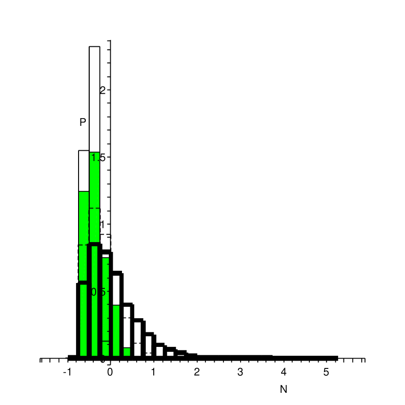
Figure 2: Frequency histogram (hist.) for the difference between solutions for different running of the spectral index, i.e. different $n_{a}$ (spectral index at wave vector $k^{a}=0.002$Mpc^-1) and $n_{b}$ (spectral index at wave vector $k^{b}=1$Mpc^-1). Thick solid hist. gives the results for { $0<n_{a}-1<0.3$ , $-0.3<n_{b}-1<0$}; dashed hist. for { $0.075<n_{a}-1<0.3$, $-0.3<n_{b}-1<-0.075$}; the green hist. for {$0.15<n_{a}-1<0.3$ , $-0.3<n_{b}-1<-0.15$}; the solid hist. for {$0.225<n_{a}-1<0.3$ , $-0.3<n_{b}-1<-0.225$}. The area under each histogram is normalized to unit area.

Our final histogram can be seen in Fig. 2 and its distributional characterization can be seen in Table 1. To have a measure of how $\Delta N$ clusters around zero we followed this procedure: a) we have divided $\Delta N$ in the range $[-1,5.25]$ into 25 intervals of width 0.25 each containing $n_{i}$ models and then calculated for each of these intervals the average $\langle{\Delta N}\rangle_{i}$ for the models in that interval and the standard deviation $\sigma_{\Delta N_{i}}=\frac{1}{\sqrt{n_{i}}}$ ; b)we calculated $m_{2}=\Sigma_{i=1}^{25}\frac{\langle{\Delta N}\rangle^{2}_{i}}{\sigma^{2}_{\Delta N_{i}}}$, a weighted second order moment around 0 of the 25 averages of $\langle{\Delta N}\rangle_{i}$ for the intervals defined above, using the inverse of the corresponding variance $\sigma_{\Delta N_{i}}$ as weight. We also similarly calculated the weighted standard deviation $\sigma_{m_{2}}$. The total number of slow roll models we considered to construct the histogram was around $10^{7}$, and the number of models fulfilling the cuts is shown in the $N_{md}$ column of Tbl. 1.

$k=0.002Mpc^{-1}$	$k=1Mpc^{-1}$	$m_{2}$	$\sigma_{m_{2}}$	$\langle\Delta N\rangle$	$\sigma_{\Delta N}$	$P(\langle\Delta N\rangle\pm 2\sigma_{\Delta N})$	$N_{md}$
$0<n_{s}-1<0.3$	$-0.3<n_{s}-1<0$	0.644	0.022	-0.073	0.643	0.961	2366
$0.075<n_{s}-1<0.3$	$-0.3<n_{s}-1<-0.075$	0.395	0.023	-0.184	0.356	0.964	880
$0.15<n_{s}-1<0.3$	$-0.3<n_{s}-1<-0.15$	0.416	0.032	-0.338	0.25	0.956	203
$0.225<n_{s}-1<0.3$	$-0.3<n_{s}-1<-0.225$	0.462	0.036	-0.450	0.12	0.968	31

Table 1: Basic distributional characterization of Fig. 2. $m_{2}=\sqrt{\langle(\Delta N)^{2}\rangle}$ characterizes the deviation from 0. $P(\langle\Delta N\rangle\pm 2\sigma_{\Delta N})$ is the fraction of the models within 2$\sigma_{\Delta N}$ of $\langle\Delta N\rangle$. $N_{md}$ is the number of models analyzed for the given range of the $n_{s}$.

Notice in Table 1 that both $|\langle\Delta N\rangle\pm\sigma_{\Delta N}|<1$ and $|m_{2}\pm\sigma_{m_{2}}|<1$ regardless of the strength of running. The column labeled “ $P(\langle\Delta N\rangle\ \pm 2\sigma_{\Delta N})$” quantifies (at least with respect to our choice of model sampling) the extent to which we should expect a coincidence between $k_{1}$ and $k_{2}$: i.e. we should expect with roughly “95% confidence” that the length scale for which the tensor to scalar ratio reaches a minimum will coincide with the length scale for which the $n_{s}-1=0$ up to a factor of about 2 and $k_{1}>k_{2}$ (i.e. wavelength at which the tensor to scalar ratio reaches a minimum is longer than the wavelength at which $n_{s}-1$ goes through a zero). As far as the effect of different strengths of running is concerned, one sees in Table 1 that stronger running corresponds to a larger magnitude of $|\langle\Delta N\rangle|$ and a more negative value of $\langle\Delta N\rangle$. Although “statistically” marginal, the smaller $\sigma_{\Delta N}$ means that strong running seems to narrow the distribution of $\Delta N$.

IV Discussion and Conclusions

In this paper, we have studied the robustness of the approximate condition suggested by Chung:2003iu . We have quantified distributionally the extent to which one should consider the approximate consistency condition to be a prediction of single field slow roll inflation. We find that if the spectrum runs from blue to red, we should look for an approximate coincidence between the wave vector $k_{1}$ satisfying $n_{s}(k_{1})-1=0$ and the wave vector $k_{2}$ satisfying $\epsilon^{\prime}(k_{2})=0$, up to a factor of about 2. According to a WMAP analysis Peiris:2003ff , this should occur at $k/a_{0}\sim 0.02\mbox{Mpc}^{-1}$.

Given that the consistency condition is only approximate, even if one finds that observations contradict the consistency condition (for example, if observations deduce $k_{1}/k_{2}<1$) it will be very difficult to make any rigorous conclusions about the models of inflation. Furthermore, given that we have sampled each of the initial condition ranges with equal weight, it is not clear what the distribution that we computed has to do with the real world. (A similar argument can be made about much of the current literature that use similar sampling Peiris:2003ff ; Kinney:2003uw ; Dodelson:1997hr ; Boyle:2005ug .) Nonetheless, if this set of initial sampling turns out to be a good approximation to the real inflationary model distributions coming from a more fundamental theory, tests coming from this kind of approximate consistency condition may be useful. To turn this around, there may be a way to classify the vacua of more fundamental theories according to whether they satisfy roughly equal probability sampling of the slow roll initial condition or whether they prefer a very specific distribution which makes the approximate consistency condition more (or less) stringent.

Before concluding, let us briefly consider the measurement prospects for the approximate consistency condition. According to current ideas of anticipated measurements Kamionkowski:1996ks ; Kamionkowski:1996zd ; Zaldarriaga:1996xe ; Seljak:1996ti , B-mode polarization observations are necessary to reliably infer the tensor perturbation amplitudes. As is well known, B-mode polarization has the advantage over the E-mode polarization in that at the last scattering surface, the B-mode polarization cannot be generated by scalar perturbations alone because to leading order, the scalar perturbations do not generate nonzero $\{l=2,m=\pm 2\}$ amplitudes in the temperature anisotropy while the tensor modes can. Hence, in principle, assuming no large contamination from vector perturbations, B-mode polarization measurement offers a direct way to infer tensor perturbation amplitudes.

The difficulty with measuring the B-mode polarization spectrum coming from gravity waves is that because its amplitude is proportional to the local quadrupole anisotropy induced by the time derivative $\dot{h}$ (where $h$ is the amplitude of the gravitational wave) localized at the last scattering surface (due to the requirement of Thomson scattering), its amplitude is suppressed at least by order $k/(a_{R}H_{R})$ on long wavelengths with respect to the temperature anisotropy (where $H_{R}$ and $a_{R}$ are the Hubble radius and the scale factor at recombination, respectively). Furthermore, since gravitational wave mode amplitudes inside the horizon are diluted by the expansion of the spatial volume, the transfer function should behave approximately as $\frac{1}{1+(\frac{k}{a_{0}})^{2}(\frac{a_{R}}{a_{0}})\frac{1}{H_{0}^{2}}}$ where $a_{0}$ is the scale factor today and $a_{R}/a_{0}\sim 10^{3}$ is the redshift to the last scattering surface. (Here, we have considered only the modes that entered the horizon after matter domination, i.e. $k/a_{0}<H_{0}\sqrt{a_{0}/a_{eq}}$.) Hence, the B-polarization temperature perturbation amplitude can be written as

$$k^{3/2}\Theta_{B,l}(k)\sim 10^{-1}\frac{k}{a_{R}H_{R}}\frac{\sqrt{P_{h}(k)}}{1+(\frac{k}{a_{0}})^{2}(\frac{a_{*}}{a_{0}})\frac{1}{H_{0}^{2}}}j_{l}(3.5k/(a_{0}H_{0}))$$ (49)

where $P_{h}$ is the power spectrum of the tensor perturbations. (For discussions of analytic treatments of CMB polarization, see e.g. Hu:1997hp ; Pritchard:2004qp ; Hu:1997mn ; seljaknotes ; dodelsonbook .) This peaks at $k/a_{0}=H_{0}\sqrt{a_{0}/a_{*}}\sim 1/(100\mbox{Mpc})$, and even there, the amplitude is suppressed by about $10^{-2}$ relative to the temperature anisotropies if the tensor perturbation amplitude is about the same as scalar perturbations amplitudes.

To make the situation slightly worse, $k_{1}$ is expected to be at around $k_{1}/a_{0}\sim 1/(50\mbox{Mpc})$. (Note that to map the wave vectors $k/a_{0}$ to the multipole moment number $l$, one can use the approximate formula $\frac{k}{a_{0}}\sim\frac{l}{3.5}H_{0}\approx\frac{l}{15,000\mbox{ Mpc}}$.) This means that to actually measure $k_{1}/k_{2}$, one must go to short scales ($l\sim 300$) while the B-mode polarization measurements prefer large length scales ($l\sim 90$; for more accurate plots of examples, see e.g. Knox:2002pe ; Cooray:2005xr ). Hence, experimental confirmation of the approximate consistency conditions will be a challenge.

There is one more obstacle that makes it difficult for tensor perturbation amplitudes to be extracted from B-mode polarization measurements. This is due to the fact that E-modes can be converted into B-modes through gravitational lensing Zaldarriaga:1998ar ; Seljak:2003pn . Hence, obtaining a tensor spectrum to check the approximate consistency condition requires success in extracting the tensor perturbation contribution even at relatively short length scales, around where the lensing contribution most likely dominates over the gravitational wave signal. This contamination from gravitational lensing can be subtracted out, at least in principle, if the lens distribution can be accurately deduced.

Despite the difficulties, we are optimistic that the ingenuity of researchers in the future will allow a test of the approximate consistency conditions considered here.

V Acknowledgment

We thank Niayesh Afshordi and Scott Dodelson for useful discussions and helpful, detailed comments on the manuscript.

Appendix A Slow Roll Formulae

Here we report some formulas which can be used to express slow roll parameters in terms of $\epsilon$ and its derivatives respect to the field $\phi$ or the operator $d\over dN$. Denoting $\frac{d\epsilon}{d\phi}=\epsilon^{{}^{\prime}}$ and $\frac{d\epsilon}{dN}=\dot{\epsilon}$ :

$$\eta = {\frac{4\,{{\epsilon}}^{3/2}\pi+{\epsilon^{{}^{\prime}}}\,\sqrt{\pi}m}{4\pi\,\sqrt{{\epsilon}}}}$$ (50)

$$\sigma = {\frac{-4\,{{\epsilon}}^{3/2}\pi+{\epsilon^{{}^{\prime}}}\,\sqrt{\pi}M_{p}}{2\pi\,\sqrt{{\epsilon}}}}$$ (51)

$${}^{2}\lambda_{\rm H} = {\frac{16\,\pi\,{{\epsilon}}^{3}+12\,{{\epsilon}}^{3/2}\sqrt{\pi}{\epsilon^{{}^{\prime}}}\,M_{p}-{{\epsilon^{{}^{\prime}}}}^{2}{M_{p}}^{2}+2\,{\epsilon^{{}^{\prime\prime}}}\,{M_{p}}^{2}{\epsilon}}{{16\pi\epsilon}\ }}$$ (52)

$$\eta = {\frac{\pi\,\left(2\,{{\epsilon}}^{2}+{\dot{\epsilon}}\right)}{2\pi\,{\epsilon}}}$$ (53)

$$\sigma = \frac{\dot{\epsilon}-2\epsilon^{2}}{\epsilon}$$ (54)

$${}^{2}\lambda_{\rm H} = {\frac{2\,{{\epsilon}}^{4}+3\,{{\epsilon}}^{2}{\dot{\epsilon}}-{{\dot{\epsilon}}}^{2}+{\ddot{\epsilon}}\,{\epsilon}}{{2{\epsilon}}^{2}}}$$ (55)

References

- (1) A. Vallinotto, E. J. Copeland, E. W. Kolb, A. R. Liddle and D. A. Steer, “Inflationary potentials yielding constant scalar perturbation spectral indices,” Phys. Rev. D 69, 103519 (2004) [arXiv:astro-ph/0311005].
- (2) H. V. Peiris et al., Astrophys. J. Suppl. 148, 213 (2003) [arXiv:astro-ph/0302225].
- (3) U. Seljak et al., Phys. Rev. D 71, 103515 (2005) [arXiv:astro-ph/0407372].
- (4) C. L. Bennett et al., Astrophys. J. Suppl. 148, 1 (2003) [arXiv:astro-ph/0302207].
- (5) W. J. Percival et al. [The 2dFGRS Collaboration], Mon. Not. Roy. Astron. Soc. 327, 1297 (2001) [arXiv:astro-ph/0105252].
- (6) J. E. Lidsey, A. R. Liddle, E. W. Kolb, E. J. Copeland, T. Barreiro and M. Abney, Rev. Mod. Phys. 69, 373 (1997) [arXiv:astro-ph/9508078].
- (7) D. J. H. Chung, G. Shiu and M. Trodden, Phys. Rev. D 68, 063501 (2003) [arXiv:astro-ph/0305193].
- (8) W. H. Kinney, E. W. Kolb, A. Melchiorri and A. Riotto, Phys. Rev. D 69, 103516 (2004) [arXiv:hep-ph/0305130].
- (9) L. Knox and Y. S. Song, Phys. Rev. Lett. 89, 011303 (2002) [arXiv:astro-ph/0202286].
- (10) A. Cooray, arXiv:astro-ph/0503118.
- (11) S. Dodelson, W. H. Kinney and E. W. Kolb, inflation Phys. Rev. D 56, 3207 (1997) [arXiv:astro-ph/9702166].
- (12) L. A. Boyle, P. J. Steinhardt and N. Turok, arXiv:astro-ph/0507455.
- (13) T. Banks, M. Dine and E. Gorbatov, JHEP 0408, 058 (2004) [arXiv:hep-th/0309170].
- (14) A. R. Liddle, P. Parsons, and J. D. Barrow, Phys. Rev. D 50, 7222 (1994) [arXiv:astro-ph/9408015].
- (15) A. C. Hindmarsh, “ODEPACK, A Systematized Collection of ODE Solvers,” in Scientific Computing, R. S. Stepleman et al. (eds.), North-Holland, Amsterdam, 1983 (vol. 1 of IMACS Transactions on Scientific Computation), pp. 55-64 [http://www.netlib.org/odepack/].
- (16) M. B. Hoffman and M. S. Turner, Phys. Rev. D 64, 023506 (2001) [arXiv:astro-ph/0006321].
- (17) D. J. Schwarz, C. A. Terrero-Escalante, and A. .A. Garcia, Phys. Lett. B517, 243 (2001), astro-ph/0106020.
- (18) W. H. Kinney, Phys. Rev. D 66, 083508 (2002), astro-ph/0206032.
- (19) E. D. Stewart and D. H. Lyth, Phys. Lett. 302B, 171 (1993).
- (20) J. E. Lidsey, A. R. Liddle, E. W. Kolb, E. J. Copeland, T. Barriero, and M. Abney, Rev. Mod. Phys. 69, 373 (1997).
- (21) A. R. Liddle. and M. S. Turner, Phys. Rev. D 50, 758 (1994).
- (22) M. Kamionkowski, A. Kosowsky and A. Stebbins, Phys. Rev. D 55, 7368 (1997) [arXiv:astro-ph/9611125].
- (23) M. Kamionkowski, A. Kosowsky and A. Stebbins, Phys. Rev. Lett. 78, 2058 (1997) [arXiv:astro-ph/9609132].
- (24) M. Zaldarriaga and U. Seljak, Phys. Rev. D 55, 1830 (1997) [arXiv:astro-ph/9609170].
- (25) U. Seljak, arXiv:astro-ph/9608131.
- (26) W. Hu and M. J. White, Phys. Rev. D 56, 596 (1997) [arXiv:astro-ph/9702170].
- (27) J. R. Pritchard and M. Kamionkowski, waves: An Annals Phys. 318, 2 (2005) [arXiv:astro-ph/0412581].
- (28) W. Hu, U. Seljak, M. J. White and M. Zaldarriaga, Phys. Rev. D 57, 3290 (1998) [arXiv:astro-ph/9709066].
- (29) Notes from Princeton University course PHY 564 course (Spring term 2004) taught by Uros Seljak (can be accessed from http://wwwphy.princeton.edu/uros/phy564.html).
- (30) S. Dodelson, Modern Cosmology (Academic Press, Boston, Mass. 2003).
- (31) M. Zaldarriaga and U. Seljak, Phys. Rev. D 58, 023003 (1998) [arXiv:astro-ph/9803150].
- (32) U. Seljak and C. M. Hirata, Phys. Rev. D 69, 043005 (2004) [arXiv:astro-ph/0310163].