Finite source effect on the polarization degree induced by a single microlens

Abstract

We investigate the effect of a single microlens on Stokes parameters. Semi-analytical formulae of the microlensed Stokes parameters are derived. The formulae not only reduce the double integrals in the estimations of those quantities but can also be approximated to a useful form in the bypass case. By using our formulation, we show that a combination of polarimetric data with photometric data enables us to estimate not only the finite source effect but also the direction of the microlens motion.

1 Introduction

The microlens effect is a phenomenon in which the flux emitted from a source (star) varies with time due to the gravitational lens effect produced by a compact object in the foreground, such as a star or a planet. Paczyǹski (1986) suggested that microlensing events could be detected by a successive observation of stars in LMC, SMC or our Galactic bulge, and since 1993 (Alcock et al., 1993; Aubourg et al., 1993; Udalski et al., 1993) many observational groups have reported a substantial number of microlensing events. According to Paczyǹski, the observations of microlensing events provide information on the mass distribution of invisible objects in galaxies; further, they impose some restrictions on the dark matter.

The observation of a microlensing event provides a light curve of the source, which is a fundamental observable in this event. From analysis of the light curve, it is important to estimate the microlens parameters such as the mass $M$ of the microlens object, the distance parameter $\zeta$($=D_{\mathrm{OL}}/D_{\mathrm{OS}}$, where $D_{\mathrm{OL}},D_{\mathrm{OS}}$ are the distances from the microlens and from the source to the observer, respectively) and relative velocity $\mn@boldsymbol{V}$ of the microlens orthogonal to the line of sight. However, it is usually very difficult to obtain the value of each parameter because these parameters are coupled with each other in observed quantities, e.g. the event duration $\hat{t}=2t_{\mathrm{E}}=2r_{\mathrm{E}}/|\mn@boldsymbol{V}|$ and the normalized minimum impact parameter $u_{0}=b/r_{\mathrm{E}}$, where $r_{\mathrm{E}}=(4GMD_{\mathrm{OS}}\zeta(1-\zeta)/c^{2})^{1/2}$ is the Einstein ring radius on the lens plane.

In order to decouple the degeneracy in the microlens parameters, several authors have proposed useful effects associated with microlens events, namely, the parallax effect on the light curve (Gould, 1992), and the accurate astrometry of the lensed source (Høg, Novikov & Polnarev, 1995; Miyamoto & Yoshii, 1995; Walker, 1995). The former effect enables us to measure the Einstein ring radius projected on the observer plane (referred to as the reduced Einstein ring radius $\tilde{r}_{\mathrm{E}}=r_{\mathrm{E}}/(1-\zeta)$). This effect has been observed in a large number of events (Alcock et al., 1995; Mao, 1999; Alcock et al., 2000; Bond et al., 2001; Mao et al., 2002; Smith et al., 2002; Smith, Mao & Paczyǹski, Smith et al.2003a; Afonso et al., 2003; Bennet et al., 2002; Smith, Mao & Wozniak, Smith et al.2003b). The latter effect provides the angular Einstein ring radius $\theta_{\mathrm{E}}(=r_{\mathrm{E}}/D_{\mathrm{OL}})$ through the observation of the fine motion of the lensed source. In order to detect this effect, we need the $\mu$as level accuracy in the astrometry. Hence, some satellite projects are being planned for carrying out such observations.These two effects are expected to impose restrictions on the determination of the microlens parameters. In particular, the detection of both the effects in the same event enables us to decouple the degeneracy in the parameters $M,\zeta$ and $|\mn@boldsymbol{V}|$ as $M=c^{2}\tilde{r}_{\mathrm{E}}\theta_{\mathrm{E}}/4G,\ \zeta=\tilde{r}_{\mathrm{E}}/(D_{\mathrm{OS}}\theta_{\mathrm{E}}+\tilde{r}_{\mathrm{E}})$ and $|\mn@boldsymbol{V}|=\zeta D_{\mathrm{OS}}\theta_{\mathrm{E}}/t_{\mathrm{E}}$, respectively.

To date, certain events that involved the estimation of the microlens mass without the high-precision astrometry have been reported (, Smith et al.2003b; Yoo et al., 2004; Park et al., 2004; Ghosh et al., 2004; Jiang et al., 2004). In four of these events, the authors (; Yoo et al.; Park et al.; Jiang et al.) not only detected the parallax effect but also estimated the angular Einstein radius by combining an empirical relation between the angular size $\theta_{*}$ and the colour-magnitude of the source given by van Belle (1999) with the finite source effect $\rho_{*}=\theta_{*}/\theta_{\mathrm{E}}$ on the light curve (Witt & Mao, 1994; Nemiroff & Wickramasinghe, 1994). The finite source effect is relatively easy to be detected in the transit case, where the lens transverses the face of the source projected on the lens plane; this is because the light curve of an extended source is significantly different from that of a point source when the normalized impact parameter $u$ is such that $u\la\rho_{*}$ (e.g. Alcock et al., 1997; Soszyński et al., 2001). The above events that are successful in decoupling the degeneracy in the parameters are examples in the case. On the other hand, in the bypass case, where the lens never transverses the face of the source, it is difficult to detect the effects because we can fit the light curve using appropriate parameters in a point source model (Gould, 1994). Gould & Welch (1995) found that in the bypass case the finite source effect is not detectable by a single-band observation but can be detected by a two-band observation, especially in the optical and infrared bands.

Recently, Simmons, Willis & Newsam (Simmons et al.1995a) and Simmons, Newsam & Willis (Simmons et al.1995b) pointed out that the finite source effect also appears in another aspect of the microlens effect. They found that the Chandrasekhar effect (Chandrasekhar, 1960) is enhanced by the microlens effect and that this enhancement causes the polarization degree of the source to vary with the motion of the microlens. They also found that the polarization degree has a double peak in the transit case, while it has a single peak in the bypass case. They presented a numerical calculation of the Stokes parameters with the microlens effect; however, they did not present the analytical formula, although the size dependence of the polarization degree helps us to decouple the degeneracy in the microlens parameters. Before , Schneider & Wagoner (1987) also discussed the gravitational lens effect on the polarization degree as a tool for identifying a lensed supernova. In their paper, by using a simple approximation of the magnification factor for a point lens, they presented a semi-analytical formula of the polarization degree and the magnification factor to demonstrate that the size expansion during the supernova explosion yields variations in these quantities. However, they did not discuss the benefits from the polarimetry of the microlensed source at all.

In this paper, we focus on the finite source effect on the Stokes parameters and the polarization degree of the microlensed star. Further, we will also discuss the possibility that the polarimetric observation of the lensed source decouples the degeneracy in the microlens parameters. Throughout this paper, we consider a single microlens. The outline of this paper is as follows. In Section 2, we provide a brief review of the microlens effect. In Section 3, we present semi-analytical formulae of the Stokes parameters to discuss the finite source effect on the polarization degree. Then, we provide an approximation of the formula with regard to the bypass case. In Section 4, we consider the extraction of information concerning the finite source effect from the polarimetric observation of the microlensed source. Finally, in Section 5, we discuss some of the possibilities of detecting the polarization induced by the microlens effect.

2 Microlens effect on the light curve

When light rays from a distant source pass near a compact object (microlens) with mass $M$, they are deflected by an angle $4GM/c^{2}b$, where $b$ is an impact parameter. Let $D_{\mathrm{OS}},D_{\mathrm{OL}}$ be the distances from the source and from the microlens to the observer, respectively. Let $\mn@boldsymbol{\theta}_{\mathrm{S}}$ be the angular position of the source that would be observed without the microlens. In this situation, the lensed light (hereafter referred to as ‘image’) is observed at the angular position $\mn@boldsymbol{\theta}$, which is obtained as a solution of the following lens equation:

$$\mn@boldsymbol{\theta}_{\mathrm{S}}=\mn@boldsymbol{\theta}-{\theta_{\mathrm{E}}^{2}\over\theta^{2}}\mn@boldsymbol{\theta},$$ (1)

where $\theta_{\mathrm{E}}=\sqrt{4GM(1-\zeta)/\zeta c^{2}D_{\mathrm{OS}}}$ is the angular Einstein ring radius. The distance parameter $\zeta$ is given by $D_{\mathrm{OL}}/D_{\mathrm{OS}}$. In equation (1), let us introduce the dimensionless variables $\mn@boldsymbol{u}\equiv\mn@boldsymbol{\theta}_{\mathrm{S}}/\theta_{\mathrm{E}}$ and $\mn@boldsymbol{x}\equiv\mn@boldsymbol{\theta}/\theta_{\mathrm{E}}$ and rewrite the lens equation as follows:

$$\mn@boldsymbol{u}=\mn@boldsymbol{x}-{\mn@boldsymbol{x}\over|\mn@boldsymbol{x}|^{2}}.$$ (2)

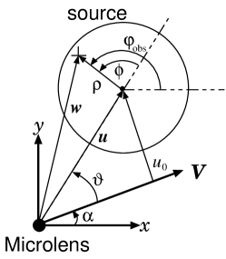
Figure 1: Geometry of microlens and source: $\mn@boldsymbol{u}$ and $\mn@boldsymbol{w}$ are the vectors to the centre and to a point marked as ‘+’ at $(\rho,\phi)$ of the source projected on the lens plane from the microlens, respectively. $\vartheta$ and $\alpha$ are the angles between $\mn@boldsymbol{V}$ and $\mn@boldsymbol{u}$ and between $\mn@boldsymbol{V}$ and the $x$–axis defined by an observer, respectively. Therefore, $\varphi_{\mathrm{obs}}=\phi+\vartheta+\alpha$ is the angle between the $x$–axis and the line joining the marked point and the centre. $u_{0}$ is the minimum impact parameter.

In general, the equation has two solutions, $\mn@boldsymbol{x}_{\pm}$, and they give the image positions of the source. One of the images is gravitationally magnified by factor $A_{+}$, while the other is magnified by factor $A_{-}$ (demagnified):

$$A_{\pm}(u)=\frac{1}{2}\left({u^{2}+2\over u\sqrt{u^{2}+4}}\pm 1\right).$$ (3)

However, we cannot resolve each image because the typical separation angle between the images is $\sim\theta_{\mathrm{E}}\la 0.1-1(M/M_{\odot})^{1/2}\mathrm{mas}$. Hence, we observe them as a single image with the following magnification factor:

$$A_{\mathrm{p}}(u)=A_{+}(u)+A_{-}(u)={u^{2}+2\over u\sqrt{u^{2}+4}}.$$ (4)

Because the microlens moves with a velocity $\mn@boldsymbol{V}$ relative to the line of sight, the normalized distance $u$ from the microlens to the source varies with time as $u=\{u_{0}^{2}+\tau^{2}\}^{1/2}$, where $u_{0}$ is the normalized minimum impact parameter of the microlens, $\tau=(t-t_{0})/t_{\mathrm{E}}$ is the time normalized by the time-scale of the microlensing event ($t_{\mathrm{E}}=D_{\mathrm{OL}}\theta_{\mathrm{E}}/|\mn@boldsymbol{V}|$) and $t_{0}$ is the time at which the magnification factor has a maximum value. Consequently, the microlens motion yields the variation of the magnification factor.

By taking into account the finite size of the source, some authors pointed out a remarkable difference between the light curves of the point source (the standard microlens) model and of the extended source model (Witt & Mao, 1994; Nemiroff & Wickramasinghe, 1994). This effect is termed the finite source effect. In general, the lensed flux is given by

$$S_{I}(\rho_{*}|u)=\int_{0}^{\rho_{*}}\theta_{\mathrm{E}}^{2}\rho\mathrm{d}\rho\int_{-\pi}^{\pi}I(\theta_{\mathrm{E}}\rho,\phi)A_{\mathrm{p}}(w(u,\rho,\phi))\mathrm{d}\phi\equiv A(\rho_{*}|u)S_{I0},\quad S_{I0}=\int_{0}^{\rho_{*}}\theta_{\mathrm{E}}^{2}\rho\mathrm{d}\rho\int_{-\pi}^{\pi}I(\theta_{\mathrm{E}}\rho,\phi)\mathrm{d}\phi,$$ (5)

where $I(r,\phi)$ is the surface brightness and $A(\rho_{*}|u)$ denotes the total magnification factor. In the above equations, $\rho$ denotes the normalized radial distance to a point on the lens plane from the centre of the projected source, while $\phi$ denotes the angle between $\mn@boldsymbol{u}$ and the line joining the point and the centre (Fig. 1). Furthermore, $\rho_{*}=\theta_{*}/\theta_{\mathrm{E}}$ ($\theta_{*}$: the angular radius of the source) is the normalized radius of the source, and $w$ is the normalized distance from the microlens to the point, given by $w(u,\rho,\phi)=\sqrt{u^{2}+2u\rho\cos\phi+\rho^{2}}$.

The total lensed flux from the extended source with axial symmetry in the surface brightness, $I(r,\phi)=I(\theta_{\mathrm{E}}\rho)$, is given by

$$S_{I}(\rho_{*}|u)=4\theta_{\mathrm{E}}^{2}\int_{0}^{\rho_{*}}\rho\mathrm{d}\rho I(\theta_{\mathrm{E}}\rho)\left[{(u-\rho)^{2}\Pi(\pi/2;k,n)+2F(\pi/2;k)\over(u+\rho)\sqrt{(u-\rho)^{2}+4}}\right],$$ (6)

where $F(\pi/2;k)$ and $\Pi(\pi/2;k,n)$ are the complete elliptical integrals of the first and of the third kinds, respectively (Gradshteyn & Ryzhik, 1996,  see also Appendix A). Further,

$$n={4u\rho\over(u+\rho)^{2}},\quad k=\sqrt{4n\over(u-\rho)^{2}+4},$$ (7)

were introduced by Witt & Mao, where the total magnification factor of the flux from the source with a constant surface brightness was estimated. An equivalent expression of equation (6) was also presented by Witt (1995), which enables us to numerically calculate the total fluxes in various bands. Using this expression, we can obtain the total magnification for the source with the limb-darkening surface brightness

$$I(\theta_{\mathrm{E}}\rho)=I_{0}\left[1-c_{1}\left(1-\sqrt{1-{\rho^{2}\over\rho_{*}^{2}}}\right)\right]$$ (8)

as follows:

$$A(\rho_{*}|u)={4\over\pi\rho_{*}^{2}(1-c_{1}/3)}\int_{0}^{\rho_{*}}\mathrm{d}\rho\rho\left[1-c_{1}\left(1-\sqrt{1-{\rho^{2}\over\rho_{*}^{2}}}\right)\right]{(u-\rho)^{2}\Pi(\pi/2;k,n)+2F(\pi/2;k)\over(u+\rho)\sqrt{(u-\rho)^{2}+4}},$$ (9)

where $c_{1}$ is a parameter that depends on the wavelength of the light.

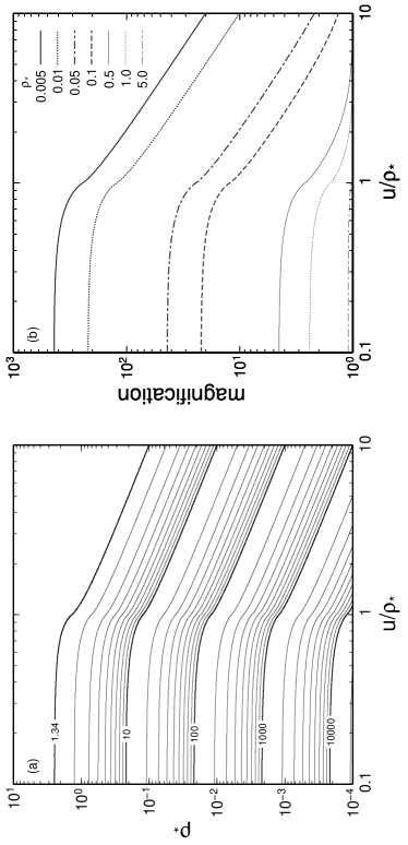
Figure 2: Magnification factor: contours of the magnification factor (a) and the $u/\rho_{*}$ dependency of the magnification factor (b). In our estimation, the linear limb-darkening model $I(\theta_{\mathrm{E}}\rho)=I_{0}\{1-c_{1}[1-(1-\rho^{2}/\rho_{*}^{2})^{1/2}]\}$ is adopted, where $c_{1}=0.64$.

In Fig. 2, we present the contours of $A(\rho_{*}|u)$ on the $u/\rho_{*}$-$\rho_{*}$ plane in panel (a) and the $u/\rho_{*}$ dependence of $A(\rho_{*}|u)$ in panel (b). Both panels clearly show that the behaviour of $A(\rho_{*}|u)$ inside the source is very different from that outside the source. Outside the source, the contours (Fig. 2-a), particularly, for low $\rho_{*}$, are almost straight lines with a slope of $\rho_{*}/u$, which shows that the magnification factors depend only on $u$. On the other hand, the contours inside the source are rather flat, which means that the factors inside the source have little dependence on $u$.

3 Microlens effect on the Stokes parameters

3.1 Stokes parameters

Chandrasekhar (1960) numerically calculated the effect of electron scattering in the atmosphere of a star on the light emitted from the star and found that it leads to polarization (the Chandrasekhar effect). According to Schneider & Wagoner (1987), we can assume that the Stokes parameters $Q,U,V$ at each point $(\rho,\phi)$ on the surface of the star with axial symmetry are expressed as follows:

$$Q(\theta_{\mathrm{E}}\rho)=I_{0}c_{2}\left(1-\sqrt{1-{\rho^{2}\over\rho_{*}^{2}}}\right),\ U=V=0.$$ (10)

Normally, we cannot resolve the light from each point on a star except for the Sun. We only observe the total flux that is obtained by integrating the lights over the surface of the star. In this case, the total Stokes parameters, $S_{Q},S_{U}$ and $S_{V}$, are also defined as those integrated over the surface. In integrating the Stokes parameters over the surface, it must be done based on the same reference frame. In this regard, we must fix $x$- and $y$- axes such as in the West and North directions, respectively. As seen in Fig. 1, we define the angle between $x$-axis defined by the observer and the line joining the centre of the star and the point $(\rho,\phi)$ as $\varphi_{\mathrm{obs}}$. We thus define the total Stokes parameters as follows:

$$\left(\begin{array}[]{c}S_{Q}\\ S_{U}\\ S_{V}\end{array}\right)=\int_{0}^{\rho_{*}}\theta_{\mathrm{E}}^{2}\rho\mathrm{d}\rho Q(\theta_{\mathrm{E}}\rho)\int_{-\pi}^{\pi}\mathrm{d}\varphi_{\mathrm{obs}}\left(\begin{array}[]{c}\cos 2\varphi_{\mathrm{obs}}\\ -\sin 2\varphi_{\mathrm{obs}}\\ 0\end{array}\right).$$ (11)

In this case, we can easily deduce that $S_{Q}=S_{U}=S_{V}=0$ because of the axial symmetry. Therefore, the light from the usual circular star is unpolarized. Specifically, we cannot detect the Chandrasekhar effect in a star without any symmetry breaking. In fact, Kemp et al. (1983) detected this effect during an eclipse in a binary system.

3.2 Microlensing on polarization

(Simmons et al.1995a) pointed out that due to the symmetry breaking by the differential gravitational magnification, the cancellation of polarization between symmetrical points on the surface is incomplete, and the flux is totally polarized as a result. Moreover, the magnification of light from each part of the surface also varies with the microlens motion. Consequently, the polarization varies with time. (Simmons et al.1995b) also numerically calculated the polarization degree and found that the time profile of the polarization has a single peak in the bypass case, while it has double peaks in the transit case. Unfortunately, it is difficult to understand the finite source effect on polarization, especially the size dependence of polarization, only on the basis of the numerical calculation.

According to (Simmons et al.1995b), the lensed Stokes parameters are given by

$$\left(\begin{array}[]{c}S_{Q}\\ S_{U}\end{array}\right)=\int_{0}^{\rho_{*}}\theta_{\mathrm{E}}^{2}\rho\mathrm{d}\rho Q(\theta_{\mathrm{E}}\rho)\int_{-\pi}^{\pi}\mathrm{d}\varphi_{\mathrm{obs}}\left(\begin{array}[]{c}\cos 2\varphi_{\mathrm{obs}}\\ -\sin 2\varphi_{\mathrm{obs}}\end{array}\right)A_{\mathrm{p}}(w(u,\rho,\phi)).$$ (12)

The relation between $\varphi_{\mathrm{obs}}$ and $\phi$ is $\varphi_{\mathrm{obs}}=\phi+\vartheta+\alpha$, where $\vartheta=-\tan^{-1}(u_{0}/\tau)$ and $\alpha$ is the angle between the direction of the microlens motion $\mn@boldsymbol{V}$ and the $x$-axis (see Fig. 1). From this relation, we can integrate the inner part of equation (12) with respect to $\phi$ and express the Stokes parameters as follows:

$$\left(\begin{array}[]{c}S_{Q}\\ S_{U}\end{array}\right) = D(\rho_{*}|u)\left(\begin{array}[]{c}\cos 2(\vartheta+\alpha)\\ -\sin 2(\vartheta+\alpha)\end{array}\right),$$ (17)

$$D(\rho_{*}|u) = 4I_{0}\theta_{\mathrm{E}}^{2}c_{2}\int_{0}^{\rho_{*}}\mathrm{d}\rho\left(1-\sqrt{1-{\rho^{2}\over\rho_{*}^{2}}}\right)\left[{(u-\rho)^{2}\over u^{2}\rho(u+\rho)\sqrt{(u-\rho)^{2}+4}}\Pi({\pi/2};k,n)\right.$$ (18)

$$\hskip 5.69054pt+{(u^{2}-\rho^{2})^{2}(u^{2}+\rho^{2})+6(u^{4}+\rho^{4})+4u^{2}\rho^{2}\over 8u^{2}\rho(u+\rho)\sqrt{(u-\rho)^{2}+4}}F({\pi/2};k)\left.-{(u+\rho)(u^{2}+\rho^{2}+2)\sqrt{(u-\rho)^{2}+4}\over 8u^{2}\rho}E({\pi/2};k)\right],$$

where $E(\pi/2;k)$ is the complete elliptical integral of the second kind; $k$ and $n$ are given by equation (7). Hence, we obtain the polarization degree as follows:

$$P(\rho_{*}|u)={\sqrt{S_{Q}^{2}+S_{U}^{2}}\over S_{I}(\rho_{*}|u)}={D(\rho_{*}|u)\over S_{I}(\rho_{*}|u)}.$$ (19)

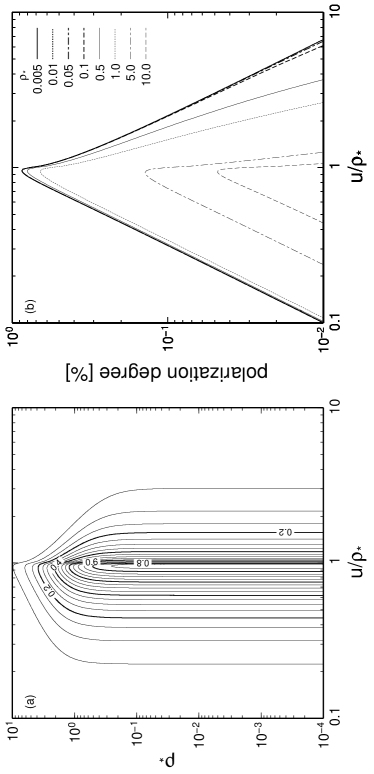
Figure 3: Polarization degree: Contours of the polarization (a) and the $u/\rho_{*}$ dependency of the polarization degree (b). In this estimation, the limb-darkening model $Q(\theta_{\mathrm{E}}\rho)=I_{0}c_{2}[1-(1-\rho^{2}/\rho_{*}^{2})^{1/2}]$ is adopted, where $c_{2}=0.04$. In panel (a), the contour spacing is 0.05 per cent.

Using equations (6) and (18), we can reduce the estimation of the polarization degree from a double integral to a single integral in equations (5) and (12). In the numerical estimation, we can use some subroutines (e.g. GNU Scientific Library) for the complete elliptical integrals in the these equations.

Fig. 3 shows the contours of polarization degree on the $u/\rho_{*}$-$\rho_{*}$ plane in panel (a) and the $u/\rho_{*}$-dependence on the polarization degree in panel (b). From panel (a), it is clear that for $\rho_{*}\la 0.05$, the contours are parallel to the $\rho_{*}$-axis at least up to $u/\rho_{*}\la 10$. This means that the polarization degree depends only on $u/\rho_{*}$ for $\rho_{*}\la 0.05$ and $u/\rho_{*}\la 5$, which is also shown in panel (b). As mentioned in Schneider & Wagoner, we also confirm that the polarization degree has the maximum value $P_{\mathrm{max}}\approx 0.875~{}\mathrm{per~{}cent}$ at $u/\rho_{*}\approx 0.96$ for low $\rho_{*}$. On the other hand, for large $\rho_{*}$, it is apparent from panel (b) that the polarization degree strongly depends on the star’s radius. From panel (b), furthermore, we observe that while for $u/\rho_{*}<1$, the polarization is almost proportional to $(u/\rho_{*})^{2}$, as shown by Schneider & Wagoner, whereas for $u/\rho_{*}>1$, the behaviour of the polarization is not as simple as argued by them. This difference arises due to the fact that Schneider & Wagoner adopted an approximation to the magnification factor for the point lens, while we refrained from doing this in this stage. Our expression (eq. [18]) is the exact form for the single microlens.

3.3 Polarization degree in the bypass case

The use of equations (6) and (17), besides reducing the double integral in equations (5) and (12), is also advantageous in obtaining an approximation of the polarization degree in the bypass case. Hence, in this subsection, we focus on the polarization degree in the bypass case. By using equations (A1)-(A3) given in the Appendix of Witt & Mao (1994), we can expand the complete elliptic integrals with respect to $k$ and $n$ in the bypass case ($\rho_{*}<u_{0}$ and $\rho_{*}<1$). We can thus approximate formulae (6) and (18) as follows:

$$S_{I}(\rho_{*}|u) = A_{\mathrm{p}}(u)S_{I0}\left[1+{60-28c_{1}\over 15-5c_{1}}{u^{2}+1\over\left(u^{2}+2\right)\left(u^{2}+4\right)^{2}}\left({\rho_{*}\over u}\right)^{2}\right],$$ (20)

$$D(\rho_{*}|u) = {7c_{2}\over 5(1-c_{1}/3)}{A_{\mathrm{p}}(u)S_{I0}\over\left(u^{2}+4\right)^{2}}\left({\rho_{*}\over u}\right)^{2}\left[1+{304\left(u^{6}+3u^{4}+6u^{2}+5\right)\over 147\left(u^{2}+2\right)\left(u^{2}+4\right)^{2}}\left({\rho_{*}\over u}\right)^{2}\right].$$ (21)

While the finite source effect $\rho_{*}$ is a secondary effect in the magnification factor, it is the primary effect in the polarization degree. Thus, we observe that the polarization evidently originates from the finite source effect.

Using the above equations, we can express the polarization degree in the bypass case as follows:

$$P(\rho_{*}|u)\approx{7c_{2}\over 5(1-c_{1}/3)}{\left(\rho_{*}/u\right)^{2}\over\left(u^{2}+4\right)^{2}}\left\{1+\left[{304\over 147}{u^{6}+3u^{4}+6u^{2}+5\over(u^{2}+2)(u^{2}+4)^{2}}-{60-28c_{1}\over 15-5c_{1}}{u^{2}+1\over(u^{2}+2)(u^{2}+4)^{2}}\right]\left({\rho_{*}\over u}\right)^{2}\right\}.$$ (22)

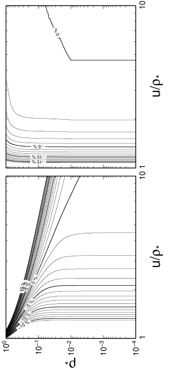
Figure 4: A Comparison of approximations to the polarization degree: The left panel shows contours of the relative errors of an approximation given by Schneider & Wagoner to the polarization degree estimated by using equations (6) and (18) numerically. The right panel shows contours of the relative errors of our approximation (22) to the numerical estimation. The contour spacing is $1~{}\mathrm{per~{}cent}$.

Equation (22) is similar to the one derived by Schneider & Wagoner; however, our approximation seems more useful even in the region $u\ga 1$. Fig. 4 present a comparison of approximation and theirs. Although both approximations deviate from the full expression (19) with a factor $1.5-2$ at $u/\rho_{*}\sim 1$, the relative error of our approximation is less than $10~{}\mathrm{per~{}cent}$ for $1.2\la u/\rho_{*}<10$ and $\rho_{*}<0.1$, whereas the region with the relative error less than $10~{}\mathrm{per~{}cent}$ of the one given by Schneider & Wagoner exists for $1.6\la u/\rho_{*}<10$ and $\rho_{*}<0.05$.

In the bypass case, the polarization degree has a maximum value $P_{\mathrm{max}}$ at $\tau=0$, as follows:

$$P_{\mathrm{max}}\approx{7c_{2}\over 80(1-c_{1}/3)}\left({\rho_{*}\over u_{0}}\right)^{2}\left\{1+\left[{871\over 5880}+{1\over 20(1-c_{1}/3)}\right]\left({\rho_{*}\over u_{0}}\right)^{2}\right\},$$ (23)

for $\rho_{*}\leq u_{0}\ll 1$ and $1.2<u_{0}/\rho_{*}<5$. For $c_{1}=0.64$ and $c_{2}=0.04$ (Schneider & Wagoner), we obtain the maximum value of the polarization degree, $P_{\mathrm{max}}\approx 0.12(2\rho_{*}/u_{0})^{2}~{}\mathrm{per~{}cent}$. This value is very small, but not always undetectable. In fact, a polarization degree of this order was detected by Kemp et al., who obtained the polarization degree $\sim 0.01~{}\mathrm{per~{}cent}$ during an eclipse in a binary system.

4 Extraction of the finite source effect from polarization

In the previous section, we investigated the polarization by a microlensing event. As mentioned in Introduction, combining the finite source effect with the parallax effect enables us to decouple the degeneracy in the microlens parameters. In this section, we shall consider the method of extracting information on the finite source effect from the polarization.

4.1 Variability of the polarization degree

(Simmons et al.1995b) showed that the polarization degree varies with time by a microlensing event and that the time profiles (variabilities) are classified into two cases, i.e. transit case and bypass case. We thus discuss the finite source effect on the polarization degree separately for each case.

4.1.1 Transit case

In the transit case, the polarization degree has a double-peak profile. Therefore, we can measure the peak times $t_{1},t_{2}(>t_{1})$ from the polarimetric observation. According to Schneider & Wagoner (1987), it is theoretically known that the polarization degree has peaks near $u=0.96\rho_{*}$. Thus, by combining $\Delta t=t_{2}-t_{1}$ with the analysis from the light curve ($u_{0},t_{\mathrm{E}}$), we can estimate $\rho_{*}$ as follows:

$$\rho_{*}\approx 1.04\sqrt{u_{0}^{2}+\left({\Delta t\over 2t_{\mathrm{E}}}\right)^{2}}.$$ (24)

4.1.2 Bypass case

Unfortunately, the polarization has only one peak in the bypass case. Hence, we cannot measure $\Delta t$, which is possible in the transit case. However, we may be able to use equation (22) to estimate $\rho_{*}$. Provided that $\rho_{*}$ has a small value and $1<u/\rho_{*}\la 5$, we can approximate the equation as follows:

$$P={a\over u^{2}}\left(1+{b\over u^{2}}\right),\ a={7c_{2}\rho_{*}^{2}\over 80(1-c_{1}/3)},\ b=\left[{871\over 5880}+{1\over 20(1-c_{1}/3)}\right]\rho_{*}^{2}.$$ (25)

Using the same approximation, we can deduce $A(\rho_{*}|u)/A_{\mathrm{p}}(u)$ from equation (20) as

$${A(\rho_{*}|u)\over A_{\mathrm{p}}(u)}=1+\left[{7\over 40}-{1\over 20(1-c_{1}/3)}\right]\left({\rho_{*}\over u}\right)^{2}\equiv 1+{c\over u^{2}},\ c=\left[{7\over 40}-{1\over 20(1-c_{1}/3)}\right]\rho_{*}^{2}.$$ (26)

Therefore, we can obtain the values of $a,b,c$ from the data fitting of the light curve and the variability of the polarization degree in the same event. Consequently, the coefficients $a,b,c$ yield $\rho_{*}$, $c_{1}$ and $c_{2}$ as follows:

$$\rho_{*}=\sqrt{{294\over 95}(b+c)},\ c_{1}={15(147b-233c)\over 1029b-871c}\ \mbox{and}\ c_{2}={7600a\over 7(1029b-871c)}.$$ (27)

4.2 $\mn@boldsymbol{u/\mn@boldsymbol{\rho}_{*}}$ dependence of polarization for small $\mn@boldsymbol{\mn@boldsymbol{\rho}_{*},u}$

As mentioned in subsection 3.2, for small $\rho_{*}$ and $u$, the polarization degree depends only on $u/\rho_{*}$. From equations (6) and (18), as well, we can prove the validity of this statement. In these equations, the arguments of the complete elliptical integrals, $k$ and $n$ are approximated as $k^{2}\approx n=4t/(1+t)^{2}$ for $\rho,u\ll 1$ (but $0<t=\rho/u<\infty$). By using the relation $(u-\rho)^{2}\Pi(\pi/2;k,n)\approx(\rho+u)^{2}E(\pi/2;k)$ derived from equation (40) in Appendix A, we find that $F(\pi/2;k)$ terms are the leading terms in the integrands of equations (6) and (18). Therefore, we can approximate these equations as follows:

$$S_{I}(\rho_{*}|u) \approx {4S_{I0}\over\pi(1-c_{1}/3)}{u\over\rho_{*}^{2}}\int_{0}^{\rho_{*}/u}\mathrm{d}t\left\{1-c_{1}\left[1-\sqrt{1-(ut/\rho_{*})^{2}}\right]\right\}{tF(\pi/2;k(t))\over 1+t},$$ (28)

and

$$D(\rho_{*}|u) \approx {4c_{2}S_{I0}\over\pi(1-c_{1}/3)}{u\over\rho_{*}^{2}}\int_{0}^{\rho_{*}/u}\mathrm{d}t\left[1-\sqrt{1-(ut/\rho_{*})^{2}}\right]{(3t^{4}+2t^{2}+3)F(\pi/2;k(t))\over 8t(1+t)}.$$ (29)

From these equations, we have proved that $P(\rho_{*}|u)=D(\rho_{*}|u)/S_{I}(\rho_{*}|u)$ depends only on $u/\rho_{*}$ for $\rho_{*},u\ll 1$.

Figure 5: $QU$ plots in transit cases (a) and in bypass cases (b): In both cases the source size $\rho_{*}=10^{-3}$ and the direction of the relative velocity $\mn@boldsymbol{V}$ is assumed to be parallel to the observer’s $x$-axis ($\alpha=0$). In the left panel, the ratios of $u_{0}$ to $\rho_{*}$ are 0.9, 0.8, 0.7, 0.6, 0.5, 0.4, 0.3, 0.2 and 0.1 from the leftmost curve. In the right panel, they are obtained as 1.1, 1.2, 1.3, 1.4, 1.5, 1.6, 1.7, 1.8, 1.9 and 2.0 from the outer curve.

Hence, we define the normalized Stokes parameters $\widehat{S}_{Q}$ and $\widehat{S}_{U}$ as

$$\widehat{S}_{Q}=S_{Q}/S_{I}=P(\rho_{*}|u)\cos 2(\vartheta+\alpha)\ \mbox{and}\ \widehat{S}_{U}=S_{U}/S_{I}=-P(\rho_{*}|u)\sin 2(\vartheta+\alpha),$$ (30)

respectively, where $\vartheta=-\tan^{-1}u_{0}/\tau$ and $\alpha$ is the direction of $\mn@boldsymbol{V}$ to the $x$-axis. Then, we can draw $QU$ plots for some values of $u_{0}/\rho_{*}$. We have presented various $QU$ plots for various $u_{0}/\rho_{*}$ values in Fig. 5, where for all the curves, we employ the same values of $\rho_{*}$ and $\alpha$; $\rho_{*}=0.001$ and $\alpha=0$. These curves are very different from each other. In particular, the curves in the transit case (panel (a)) differ considerably from those in the bypass case (panel (b)). As long as $\rho_{*}\ll 1$, however, we can specify the shapes of these curves by one parameter, $u_{0}/\rho_{*}$, because the polarization degree depends only on the parameter $u/\rho_{*}$ for small $\rho_{*}$. Hence, if we can fit the data of the Stokes parameters on an appropriately scaled curve, we can estimate $u_{0}/\rho_{*}$.

Besides the possibility of estimating $\rho_{*}$, we should note that the $QU$ plot provides information on the direction of the relative microlens motion $\mn@boldsymbol{V}$. Microlensed $QU$ plots are shown in Fig. 6 (panel (a)), in the cases when the microlenses move along lines inclined to the observer’s $x$-axis with an angle $\alpha=15^{\circ}$ (panel (b)). In these cases, we find that the plots lean at an angle $-2\alpha$ as compared to the ones with $\alpha=0$ (as shown in Fig. 5). In Fig. 6, we draw the slanted $QU$ plots for three cases: when the microlens moves from the lower-left corner to the right in panel (b) in the bypass case ($u_{0}=0.0015$), the same movement in the transit case ($u_{0}=0.0003$) and when it moves from the left to the upper-right corner in the bypass case ($u_{0}=0.0012$). While, in the first two cases, a point on the $QU$ plot moves clockwise around the origin with time, in the last case, the point moves anti-clockwise. Hence, we find that points on the $QU$ plots, in general, move anti-clockwise when the vector $\mn@boldsymbol{u}\times\mn@boldsymbol{V}$ points to the observer from the lens plane, and vice versa.

Thus, if we have data on the Stokes parameters, i.e. $(S_{I},S_{Q},S_{U})$ during a microlensing event, we can obtain not only the finite source effect $\rho_{*}$ but also the direction of the relative microlens motion, including the sign of $\mn@boldsymbol{u}\times\mn@boldsymbol{V}$.

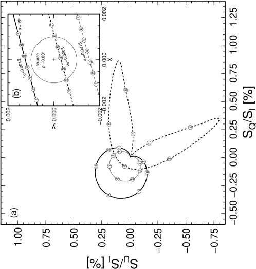
Figure 6: $QU$ plots and the corresponding trajectories of the microlenses: When the microlens moves from 1 to 7 on each line in panel (b), the point on the $QU$ plot moves from 1 to 7 on the corresponding curve in panel (a). In this figure, it is assumed that $\rho_{*}=10^{-3}$ and the lines are inclined to the $x$-axis with $\alpha=15^{\circ}$. The time interval between the circled points is $5\times 10^{-4}t_{\mathrm{E}}$.

5 Summary and Discussion

In this paper we have investigated the single microlens effect on the Stokes parameters in order to obtain some semi-analytical formulae. As a result, we observe that the formulae not only reduce the double integrals in the estimations of the parameters but also can be expressed as a useful approximation form in the bypass case. In addition, we have shown that by combining the polarimetric data with photometric data, we can estimate not only the finite source effect $\rho_{*}$ but also the direction of the microlens motion, including the sign of $\mn@boldsymbol{u}\times\mn@boldsymbol{V}$.

Although we have argued on the benefits of observations of polarized stars by the microlensing event, we have not yet enumerated the difficulties involved in the polarimetric observation of the microlensed star. In this regard, we shall comment on the following difficulties in the remainder of this paper: (1) the lower limit of the detectable polarization degree, (2) the limiting magnitude of the polarimetric observation, (3) the observable duration for polarization and (4) the identification of the target star.

The first difficulty is concerned with observational technology. Although Kemp et al. (1983) succeeded in measuring the polarization degree with $\sim 0.01~{}\mathrm{per~{}cent}$ accuracy during an eclipse in a binary system, it is not easy to detect polarized light with such accuracy even with the present technology. At present, we can expect the accuracy of the polarization degree to be $P_{\mathrm{lim}}\approx 0.05~{}\mathrm{per~{}cent}$ (Hirata, in private communication). This limit defines the upper limit for $u$ as $u\la 3\rho_{*}$ for $\rho_{*}<0.1$ (see Fig. 3). Hence, we can define the effective radius $R$ in the polarimetric observation of a microlensed star that depends on $P_{\mathrm{lim}}$, e.g. $R\approx 3\rho_{*}$ for $P_{\mathrm{lim}}=0.05~{}\mathrm{per~{}cent}$.

The second difficulty arises due to the fact that the limiting magnitude of polarimetry is in general $5-7$ mag brighter than that of photometric observation. Most of microlensed stars have magnitudes in the range of $15-21$ mag in the photometry ($I$-band). This means that the corresponding magnitudes in the polarimetry of the star are in the range of $20-28$ mag. Therefore, in order to detect the polarization, we need a large telescope. In FOCAS of the Subaru Telescope, the limiting magnitude is 26.2 mag in the $I$-band with a 1200 s exposure (Kashikawa et al., 2002). Thus, the observation is very difficult even by using FOCAS. Fortunately, while the polarization is detectable, the magnification factor of the star is larger than $1/R$. Hence, the polarized light from the microlensed star with even the faintest magnitude may be detectable by FOCAS because the magnification factor is larger than 10 when $\rho_{*}<0.03$.

The third difficulty is associated with the exposure time for the microlensed star. For the observation of faint stars, a long exposure time is necessary. In order to extract the finite source effect, we need to observe the lensed star a number of times. Further, the total exposure time must be less than the observable duration for polarization, which is equal to the crossing time $\Delta t_{\mathrm{c}}$ of the microlens over the effective diameter ($=2R$), i.e. $2Rt_{\mathrm{E}}\approx 6\rho_{*}t_{\mathrm{E}}$. We thus obtain the lower limit of $\rho_{*}$ in the polarimetric observation of the microlensed star as follows:

$$4.6\times 10^{-3}\left({N_{\mathrm{obs}}\over 100}\right)\left({t_{\mathrm{exp}}\over 1200~{}\mathrm{s}}\right)\left({50~{}\mathrm{days}\over t_{\mathrm{E}}}\right)<\rho_{*},$$ (31)

where $N_{\mathrm{obs}}$ and $t_{\mathrm{exp}}$ denote the frequency of the observations and the exposure time, respectively.

Among the four difficulties listed above, the last one may be the most challenging. It arises from a reason specific to the microlensing event. Generally, microlensed stars are observed in very crowded regions such as our Galactic bulge, LMC and SMC. Hence, there are many stars around the target star within the same field. As $50-100$ stars can be simultaneously observed using FOCAS (Kawabata, in private communication), it may be possible to detect the polarization.

If we can overcome the above difficulties, we can estimate the finite source effect from the polarimetric observation and decouple the degeneracy in the microlens parameters by using the relation given by van Belle (1999). Even after satellite projects succeed in measuring the angular Einstein ring radius $\theta_{\mathrm{E}}$, the polarimetric observation of the microlensed star will provide useful information such as on the limb-darkening model, on the relation between angular diameter and colour-magnitude of stars (van Belle) and so on. We thus believe that it is important and worthwhile to focus attention on polarimetry in microlensing events after receiving microlens alerts such as from the Early Warning System (Udalski, 2003).

Appendix A Elliptical Integrals

The elliptical functions of the first, second and third kind ($F,E,\Pi$) are given as follows:

$$F(\phi;k) = \int_{0}^{\phi}{\mathrm{d}\theta\over\sqrt{1-k^{2}\sin^{2}\theta}}=\int_{0}^{\sin^{-1}\phi}{\mathrm{d}t\over\sqrt{(1-t^{2})(1-k^{2}t^{2})}},$$ (32)

$$E(\phi;k) = \int_{0}^{\phi}\mathrm{d}\theta\sqrt{1-k^{2}\sin^{2}\theta}=\int_{0}^{\sin^{-1}\phi}dt\sqrt{1-k^{2}t^{2}\over 1-t^{2}},$$ (33)

$$\Pi(\phi;k,n) = \int_{0}^{\phi}{\mathrm{d}\theta\over(1-n\sin^{2}\theta)\sqrt{1-k^{2}\sin^{2}\theta}}=\int_{0}^{\sin^{-1}\phi}{\mathrm{d}t\over(1-nt^{2})\sqrt{(1-t^{2})(1-k^{2}t^{2})}}.$$ (34)

Let us define the integration as follows:

$$\Lambda_{l}(t;k,n)\equiv\int_{0}^{t}{\mathrm{d}t\over(1-nt^{2})^{l}\sqrt{(1-t^{2})(1-k^{2}t^{2})}}$$ (35)

The objective in this appendix is to express $\Lambda_{l}$ as a combination of $F,E$ and $\Pi$. First, we consider the derivative of $[t\sqrt{f(t)}]/(1-nt^{2})^{l-1}$ with respect to $t$, where $f(t)=(1-t^{2})(1-k^{2}t^{2})$:

$${\mathrm{d}\ \over\mathrm{d}t}\left[{t\over(1-nt^{2})^{l-1}}\sqrt{f(t)}\right]={2(l-1)f(t)+(1/2)\left(1-nt^{2}\right)\Bigl{\{}tf^{\prime}(t)+2(3-2l)f(t)\Bigr{\}}\over\sqrt{f(t)}(1-nt^{2})^{l}},$$ (36)

We restrict ourselves to $l\geq 2$. From the definition of $\Lambda_{l}$, the first three functions, $\Lambda_{1},\Lambda_{0},\Lambda_{-1}$, are expressed by the following three complete elliptical functions,

$$\Lambda_{1}(t;k,n)=\Pi(\sin^{-1}t;k,n),\quad\Lambda_{0}(t;k,n)=F(\sin^{-1}t;k)\quad\mbox{and}\quad\Lambda_{-1}(t;k,n)=(1-\displaystyle{n\over k^{2}})F(\sin^{-1}t;k)+\displaystyle{n\over k^{2}}E(\sin^{-1}t;k),$$ (37)

respectively. We denote the numerator of equation (36) as $g(t)$

$$g(t)=2(l-1)f(t)+{1\over 2}(1-nt^{2})\left[tf^{\prime}(t)-2(2l-3)f(t)\right]=A+B(1-nt^{2})+C(1-nt^{2})^{2}+D(1-nt^{2})^{3},$$

where

$$A=2(l-1)\left(1-{1\over n}\right)\left(1-{k^{2}\over n}\right),\ B=-(2l-3)\left(1-2{1+k^{2}\over n}+3{k^{2}\over n^{2}}\right),\ C=2(l-2)\left(3{k^{2}\over n^{2}}-{1+k^{2}\over n}\right)\ \mbox{and}\ D=-(2l-5){k^{2}\over n^{2}}.$$

These coefficients enable us rewrite equation (36) as follows:

$${\mathrm{d}\ \over\mathrm{d}t}\left[{t\over(1-nt^{2})^{l-1}}\sqrt{f(t)}\right] = A{\mathrm{d}\Lambda_{l}\over\mathrm{d}t}+B{\mathrm{d}\Lambda_{l-1}\over\mathrm{d}t}+C{\mathrm{d}\Lambda_{l-2}\over\mathrm{d}t}+D{\mathrm{d}\Lambda_{l-3}\over\mathrm{d}t},$$ (38)

$$= 2(l-1)\left(1-{1\over n}\right)\left(1-{k^{2}\over n}\right){\mathrm{d}\Lambda_{l}\over\mathrm{d}t}-(2l-3)\left(1-2{1+k^{2}\over n}+3{k^{2}\over n^{2}}\right){\mathrm{d}\Lambda_{l-1}\over\mathrm{d}t}$$

$$+2(l-2)\left(3{k^{2}\over n^{2}}-{1+k^{2}\over n}\right){\mathrm{d}\Lambda_{l-2}\over\mathrm{d}t}-(2l-5){k^{2}\over n^{2}}{\mathrm{d}\Lambda_{l-3}\over\mathrm{d}t},$$

We integrate the above equation from $t=0$ to $1$ in order to obtain the following recursion:

$$2(l-1)\left(1-{1\over n}\right)\left(1-{k^{2}\over n}\right)\Lambda_{l}(1;k,n) = (2l-3)\left(1-2{1+k^{2}\over n}+3{k^{2}\over n^{2}}\right)\Lambda_{l-1}(1;k,n)$$ (39)

$$-2(l-2)\left(3{k^{2}\over n^{2}}-{1+k^{2}\over n}\right)\Lambda_{l-2}(1;k,n)+(2l-5){k^{2}\over n^{2}}\Lambda_{l-3}(1;k,n).$$

For example, in the cases of $l=2,3$, we find

$$2\left(1-{1\over n}\right)\left(1-{k^{2}\over n}\right)\Lambda_{2}(1;k,n)=\left(1-2{1+k^{2}\over n}+{3k^{2}\over n^{2}}\right)\Pi(\pi/2;k,n)+{1\over n}\left(1-{k^{2}\over n}\right)F(\pi/2;k)-{1\over n}E(\pi/2;k),$$ (40)

and

$$4\left(1-{1\over n}\right)\left(1-{k^{2}\over n}\right)\Lambda_{3}(1;k,n)=3\left(1-2{1+k^{2}\over n}+{3k^{2}\over n^{2}}\right)\Lambda_{2}(1;k,n)-2\left(3{k^{2}\over n^{2}}-{1+k^{2}\over n}\right)\Pi(\pi/2;k,n)+{k^{2}\over n^{2}}F(\pi/2;k).$$ (41)

We substitute $n=4\rho u/(u+\rho)^{2},k^{2}=4n/[(u-\rho)^{2}+4]$ into equation (39) to obtain a recursive formula as follows:

$$\Lambda_{l}(1;k,n) = \left({2l-3\over l-1}\right){\rho^{2}+u^{2}-2\over(u-\rho)^{2}}\Lambda_{l-1}(1;k,n)-\left({l-2\over l-1}\right){(\rho^{2}-u^{2})^{2}-8(\rho^{2}+u^{2})\over(\rho-u)^{4}}\Lambda_{l-2}(1;k,n)$$ (42)

$$\hskip 139.4185pt-2\left({2l-5\over l-1}\right){(\rho+u)^{2}\over(\rho-u)^{4}}\Lambda_{l-3}(1;k,n).$$

For example, in the cases of $l=2,3$, we obtain

$$\Lambda_{2}(1;k,n) = {u^{2}_{0}+\rho^{2}-2\over(u-\rho)^{2}}\Pi(\pi/2;k,n)-{1\over 2}\left({u+\rho\over u-\rho}\right)^{2}F(\pi/2;k)+{(u+\rho)^{2}\left\{(u-\rho)^{2}+4\right\}\over 2(u-\rho)^{4}}E(\pi/2;k),$$ (43)

$$\Lambda_{3}(1;k,n) = {u^{4}+4u^{2}\rho^{2}-2(u^{2}+\rho^{2})+\rho^{4}+6\over(u-\rho)^{4}}\Pi(\pi/2;k,n)-{(u+\rho)^{2}(3u^{2}+3\rho^{2}-2)\over 4(u-\rho)^{4}}F(\pi/2;k)$$ (44)

$$+{3(u+\rho)^{2}(u^{2}+\rho^{2}-2)\left\{(u-\rho)^{2}+4\right\}\over 4(u-\rho)^{6}}E(\pi/2;k).$$

References

- Afonso et al. (2003) Afonso C. et al., 2003, A&A, 404, 145
- Alcock et al. (1993) Alcock C. et al., 1993, Nat, 365, 621
- Alcock et al. (1995) Alcock C. et al., 1995, ApJ, 454, L125
- Alcock et al. (1997) Alcock C. et al., 1997, ApJ, 491, 436
- Alcock et al. (2000) Alcock C. et al., 2000, ApJ, 542, 281
- Aubourg et al. (1993) Aubourg E. et al., 1993, Nat, 365, 623
- Bennet et al. (2002) Bennet D.P. et al., 2002, ApJ, 579, 639
- Bond et al. (2001) Bond I.A. et al., 2001, MNRAS, 327, 868
- Chandrasekhar (1960) Chandrasekhar S., 1960, Radiative Transfer. Dover, New York
- Ghosh et al. (2004) Ghosh H. et al., 2004, ApJ, 615, 450
- Gould (1992) Gould A., 1992, ApJ, 392, 442
- Gould (1994) Gould A., 1994, ApJ, 421, L71
- Gould & Welch (1995) Gould A., Welch D.L., 1996, ApJ, 464, 212
- Gradshteyn & Ryzhik (1996) Gradshteyn I.S., Ryzhik I.M., 1996, Tables of Integrals, Series, and Products. Academic, New York
- Høg et al. (1995) Høg E., Novikov I.D., Polnarev A.G., 1995, A&A, 294, 287
- Jiang et al. (2004) Jiang G. et al., 2004, ApJ, 617, 1307
- Kashikawa et al. (2002) Kashikawa N. et al., 2002, PASJ, 54, 819
- Kemp et al. (1983) Kemp J.C., Henson G.D, Barbour M.S, Kraus D.J., Collins II G.W., 1983, ApJ, 273, L85
- Mao (1999) Mao S., 1999, A&A, 350, L19
- Mao et al. (2002) Mao S. et al., 2002, MNRAS, 329, 349,
- Miyamoto & Yoshii (1995) Miyamoto M., Yoshii Y., 1995, AJ, 110, 3, 1427
- Nemiroff & Wickramasinghe (1994) Nemiroff R.J, Wickramasinghe W.A.D.T., 1994, ApJ, 424, L21
- Park et al. (2004) Park B.-G. et al., 2004, ApJ, 609, 166
- Paczyǹski (1986) Paczyǹski B., 1986, ApJ, 304, 1
- (25) Schneider P., Ehlers J., Falco E.E., 1992, Gravitational Lenses. Springer-Verlag, Berlin
- Schneider & Wagoner (1987) Schneider P., Wagoner R.V., 1987, ApJ, 314, 154
- (27) Simmons J.F.L., Willis J.P., Newsam A.M., 1995a, A&A, 293, L46
- (28) Simmons J.F.L., Newsam A.M., Willis J.P., 1995b, MNRAS, 276, 182
- Smith et al. (2002) Smith M.C. et al., 2002, MNRAS, 336, 670
- (30) Smith M.C., Mao S., Pacz̀ynski B., 2003a, MNRAS, 339, 925
- (31) Smith M.C., Mao S., Woźniak P., 2003b, ApJ, 585, L65
- Soszyński et al. (2001) Soszyński I. et al., 2001, ApJ, 552, 731
- Udalski et al. (1993) Udalski A. et al., 1993, Acta Astron., 43, 289
- Udalski (2003) Udalski A., 2003, Acta Astron., 53, 291
- van Belle (1999) van Belle G.T., 1999, PASP, 111,1515
- Walker (1995) Walker M.A., 1995, ApJ, 453, 37
- Witt (1995) Witt H.J., 1995, ApJ, 449, 42
- Witt & Mao (1994) Witt H.J., Mao S., 1994, ApJ, 430, 505
- Yoo et al. (2004) Yoo J. et al., 2004, ApJ, 603, 139