Repeated X-ray Flaring Activity in Sagittarius A*

Abstract

Investigating the spectral and temporal characteristics of the X-rays coming from Sagittarius A* (Sgr A*) is essential to our development of a more complete understanding of the emission mechanisms in this supermassive black hole located at the center of our Galaxy. Several X-ray flares with varying durations and spectral features have already been observed from this object. Here we present the results of two long XMM-Newton observations of the Galactic nucleus carried out in 2004, for a total exposure time of nearly 500 $\mathrm{ks}$. During these observations we detected two flares from Sgr A* with peak 2–10 $\mathrm{keV}$ luminosities about 40 times ($L_{\rm X}$ $\sim$ 9 $\times$ $10^{34}$  erg s${}^{-1}$) above the quiescent luminosity: one on 2004 March 31 and another on 2004 August 31. The first flare lasted about 2.5 ks and the second about 5 $\mathrm{ks}$. The combined fit on the Epic spectra yield photon indeces of about 1.5 and 1.9 for the first and second flare respectively. This hard photon index strongly suggests the presence of an important population of non-thermal electrons during the event and supports the view that the majority of flaring events tend to be hard and not very luminous.

1. Introduction

Sagittarius A*, the black hole at the Galactic center, is a source of fascination and curiosity for many in the astrophysical community. There are several reasons for this, including the fact that Sgr A* provides us with the most compelling evidence to date for the existence of supermassive black holes in the universe and is the closest such object (Schödel et al. 2003; Ghez et al. 2003). Its relative proximity allows us to investigate Sgr A*’s radiative characteristics, as well as those of its nearby environment, with great detail and excellent spatial and spectral resolution in all of the accessible wavebands. In addition, unlike more typical active and bright galactic nuclei, Sgr A* is very dim and shines at less than $10^{-9}$ (Melia & Falcke , 2001) times the Eddington luminosity for an object of its mass, now thought to be $M$ $\approx$ 3.4 $\times$ $10^{6}$ $\rm{M}_{\odot}$ (Schödel et al. 2003). This faintness is itself intriguing and raises many more questions about the conditions that exist in the environment surrounding the massive black hole.

And yet, this faintness may actually be a blessing in disguise for probing the innermost regions of this object, for it points to an optically thin envelope that is almost transparent to high-energy IR and X-ray photons produced during transient events manifested within a mere handful of Schwarzschild radii ($r_{S}$ $\equiv$ $2GM/c^{2}$, or roughly 9 $\times$ $10^{11}$ $\mathrm{cm}$) of the event horizon. Thus, the Galactic centre’s supermassive black hole provides a wonderful laboratory for the study of accretion and related phenomena, including the formation and evolution of accretion disks, the causes and effects of magnetic reconnection, the emission characteristics from the acceleration of charged particles in the strong magnetic and gravitational fields, the relationship between radiation at different wavelengths, and the processes that give rise to these (see Melia & Falcke 2001 for a review).

In early 2001, the Chandra X-ray Observatory detected what we now consider to be the first X-ray counterpart (Baganoff et al. 2003) to the radio source Sgr A*. The quiescent state of this source was characterized by a power-law photon index $\Gamma$ = $2.7^{+1.3}_{-0.9}$ and a derived 2–10 $\mathrm{keV}$ luminosity of $L_{\rm X}$ = (2.2 $\pm$ 0.4) $\times$ $10^{33}$ erg s${}^{-1}$. It is thought that the same population of electrons that produce the synchrotron peak at sub-mm wavelengths give rise to this quiescent component through synchrotron self-compton (SSC) (Liu & Melia 2001; Markoff et al. 2001).

In the fall of the same year, Chandra detected the first X-ray flare from this source (Baganoff et al. , 2001). This flare lasted about 10 $\mathrm{ks}$, had a harder photon index of $\Gamma$ = 1.3 $\pm$ 0.6, and reached a peak luminosity of $L_{\rm X}$ = (1.0 $\pm$ 0.1) $\times$ $10^{35}$  erg s${}^{-1}$ (or factor 45 above the quiescent level). To this day, two additional bright flares from the direction of Sgr A*, with varying time scales and spectral features, have been detected and reported. Goldwurm et al. (2003a) reported the detection of the rising portion of a flare from Sgr A* over some 900 $\mathrm{s}$. They found a flare photon index of $\Gamma$ = 0.7 $\pm$ 0.6, compatible with the Chandra flare photon index within the errors, and they derived a peak luminosity of $L_{\rm X}$ = (5.4 $\pm$ 1.0) $\times$ $10^{34}$ erg s${}^{-1}$ (a factor 25 above quiescence). The most recent report of a flare from Sgr A* is that presented by Porquet et al. (2003). This flare was quite different from the two previous events, for it lasted roughly 2.7 $\mathrm{ks}$, had a soft spectral index ($\Gamma$ = 2.5 $\pm$ 0.3), and reached a surprisingly high peak 2–10 $\mathrm{keV}$ luminosity of $L_{\rm X}$ = (3.6 $\pm$ 0.4) $\times$ $10^{35}$ erg s${}^{-1}$. This corresponds to an unprecedented factor 160 above the source’s quiescent luminosity.

X-ray flaring activity in Sgr A* could be induced by a sudden enhancement of accretion (Liu & Melia 2002a, ), from a swift acceleration of electrons in a magnetic flare near the black hole (Liu, Petrosian, and Melia 2004), within a jet (Markoff et al. , 2001), or perhaps through some other nonthermal process within a radiatively inefficient accretion flow (Yuan, Quataert, & Narayan 2003 and 2004). Furthermore, short time scale X-ray and IR flares could be much more difficult to detect if the luminosity of Sgr A* were even slightly larger in which case the thermal SSC emission would possibly dominate over the non-thermal emission (Yuan, Quataert, & Narayan 2004). The recent detection of Sgr A* in the near-IR band in both the quiescent and flaring states (Genzel et al. , 2003), and the more recent detection of a correlated increase in near-IR and X-ray flux (Eckart et al. 2004), provide further important constraints on building a comprehensive model of this source. Although relatively few instances of detected flares from Sgr A* have been reported, there appears to be two “types” of flares—the soft and hard—and a model that can naturally explain both of these types of events is presented in Liu, Petrosian, & Melia (2004).

We here present the results of two long XMM-Newton observations of Sgr A* and the Galactic center in which we detected two flares that rose to a factor of 40 above the quiescent luminosity from the direction of the central black hole, and several other, less significant events that could also be coming from Sgr A*. Both of these observations were conducted concurrently with Integral in order to investigate possible links in the manifestation of a sudden enhanced accretion, magnetic reconnection, or other types of events in the hard X-ray (2–12 $\mathrm{keV}$) and soft gamma-ray (20–120 $\mathrm{keV}$) domains. Furthermore, a set of other observations of Sgr A* covering the radio, sub-millimeter and infrared frequencies, coordinated with the 2004 XMM-Newton large project, were also planned and partly performed, and two new transient radio sources were discovered with the VLA Bower et al.  (2005). Results from the Integral observations (Bélanger et al. , 2005) and from the overall multiwavelength campaing will be reported elsewhere. The two main flares, which we will refer to as the factor-40 flares hereafter, occurred on time scales between 2500–5000 $\mathrm{s}$ and have similar spectral characteristics. These may be added to the statistics of detected flares from Sgr A* and add weight to the interpretation that there are indeed two types of flares, bright and soft or not-so-bright and hard; and that the majority of these events are of the latter kind. A larger sample of such events is essential for constructring a more robust classification—and thus identification—of the causes for this flaring activity in Sgr A*. Furthermore, a brightening of the region around Sgr A* by a factor of $\sim$ 2 in the 2–10 $\mathrm{keV}$ band with respect to all previous XMM-Newton observations of the Galactic center is evident in both datasets. The astrometry-corrected fitted centroid of this emission coincides with the position of a bright transient lying about 3${}^{\prime\prime}$ south of Sgr A* and discovered by Chandra in the summer of 2004 (Muno et al. 2005a, ). Here we will only briefly comment on the emission characteristics of this new source, CXOGC J174540.0-290031, during the XMM-Newton observations and refer the interested reader to Porquet et al. (2005) and Muno et al. (2005b) for further details.

The structure of this paper is as follows: In §2 we describe the observations and the analysis methods used to reduce the data. In §3, we present the results of the analysis, and in §4, we discuss their possible implications and interpretations.

2. Observations and Methods of Analysis

Table 1Observation Log

ObsID	Obs Start time	Obs End time	Duration
	(UT)	(UT)	(ks)
788	2004-03-28T14:57:08	2004-03-30T04:44:00	112.6
789	2004-03-30T14:46:36	2004-04-01T04:35:49	123.4
866	2004-08-31T03:12:01	2004-09-01T16:45:58	130.1
867	2004-09-02T03:01:39	2004-09-03T16:35:35	131.4

The XMM-Newton satellite observed the Galactic center as part of a large project during revolutions 788 and 789, between 2004 March 28 and April 1, and then during revolutions 866 and 867, between 2004 August 31 and September 2 for a total exposure time of $\sim$ 490 $\mathrm{ks}$, during which the Epic Mos and PN cameras were in PrimeFullWindow and PrimeFullWindowExtended modes, respectively, during epoch 1, and in PrimeFullWindow during epoch 2. The log of the observations is presented in Table 1. We will use epoch 1 to refer to the observation period spanning ObsID 788 and 789, and epoch 2 for the one spanning ObsID 866 and 867.

We generated event lists for the Mos 1, Mos 2, and PN cameras using the emchain and epchain tasks of the XMM-Newton Science Analysis System v 6.1.0. These were subsequently filtered and used to construct images in two energy bands: 0.5–2 $\mathrm{keV}$, and 2–10 $\mathrm{keV}$. The filter on the event pattern in imaging mode, (PATTERN < = 12 for Mos, and PATTERN < = 4 for PN), ensures that only events created by X-rays and free of cosmic ray contamination are selected. Artifacts from the calibrated and concatenated datasets, as well as events near CCD gaps or bad pixels are rejected by setting (FLAG==0) as a selection criterion. A further selection on the maximum count rate in the 10–12 $\mathrm{keV}$ range (18 $\mathrm{cts/s}$) for Mos and 12–14 $\mathrm{keV}$ range (22 $\mathrm{cts/s}$) for PN was applied to exclude all periods of increased charged particle flaring activity. This stringent selection criterion was only applied to the image construction.

The heavy absorption in the direction of the Galactic center, prevents photons from this region having energies below 1.5–2 $\mathrm{keV}$ from reaching us. For this reason, we used the 0.5–2 $\mathrm{keV}$ images of foreground stars to identify counterparts for astrometric corrections, and the 2–10 $\mathrm{keV}$ image to determine the flare centroid.

2.1. Astrometry

We identified three Tycho-2 and two Chandra sources with positional uncertainties of 0${}^{\prime\prime}$ .025 and 0${}^{\prime\prime}$ .16, respectively . Of these calibration sources, three were in the central Mos CCD and two just outside of it. This is an essential point in the astrometric corrections because the positional uncertainty of a Mos CCD relative to another is $\sim$ 1${}^{\prime\prime}$ .5 and this therefore determines the minimum systematic positional uncertainty over the whole field of view. However, if we have at least three calibration sources in the central CCD, then we can reduce this systematic uncertainty for sources in that CCD.

The astrometric correction was done by first running edetect_chain using the 0.5–2 $\mathrm{keV}$ images to get a list of the detected sources with their fitted position and associated statistical uncertainty. Then, using eposcorr that optimizes the correlation between the positions of the calibration sources and their X-ray counterparts allowing for a displacement in R.A. and Decl. as well as rotation, we found the boresight corrections for the three Epic instruments. The Mos cameras have smaller pixels, and therefore a finer angular resolution than the PN instrument. We therefore used the Mos images for our astrometric study of the obervations during which the flares occured, namely ObsID 789 and 866. The results of this study are listed in Table 2 where we give the offsets and root mean square (rms) dispersion in the positions of the astrometric sources with respect to their reference positions before and after correction.

Although we performed this procedure for each individual camera as well as for the merged Mos event list we used the Mos 2 results for our analysis of the first flare (ObsID 789) and the Mos 1 for the analysis of the second (ObsID 866) since these had the smallest dispersion after boresight corrections. We found that the merged Mos image systematically yielded smaller offsets in both coordinates and that the rms dispersion remained in the range 0${}^{\prime\prime}$ .9 to 1${}^{\prime\prime}$ .2 before and after boresight corrections were applied. This behaviour is expected since the astrometric precision derived from calibrations and that rely upon the knowledge of the position of one camera with respect to the other is stated as 1${}^{\prime\prime}$ .2 (Kirsch , 2005). So even though we can generally expect smaller offsets and dispersions before corrections when using the merged Mos image as this naturally averages the astrometry of both Mos cameras, the minimum dispersion after corrections will always be around 1${}^{\prime\prime}$ .2. Unusually large dispersions can be caused by the “splitting” of one or more of the astrometric sources by a column of bad pixels as was seen in Mos 2 during ObsID 866. Astrometric corrections maximize our ability to locate sources and to distinguish a flaring source from its closest known neighbour as is our intention here.

We found that the change in position due to corrections of up to 2.7${}^{\prime\prime}$ in a given coordinate has negligible effects on the light curve and spectra that are constructed by integrating over a 10${}^{\prime\prime}$ radius around the source. This is primarily due to the shape of the instrument point spread function which is characterized by a very narrow peak and broad wings. As long as the peak is included in the extraction region then variations due to a shifted centroid are completely negligible. Each individual event list is treated separately to ensure proper good-time-interval corrections.

Table 2Astrometric Corrections

	ObsID 789	ObsID 866
R.A. offset	$-2.67\pm 0.60$	$0.88\pm 0.61$
Decl. offset	$0.35\pm 0.56$	$0.35\pm 0.46$
Rotation	$-0.20\pm 0.30$	$-0.05\pm 0.25$
RMS before correction	$3.22$	$1.40$
RMS after correction	$0.59$	$0.88$

Note. — All quantities are given in arc seconds. The column ObsID 789 lists the parameter values for Mos 2 and ObsID 866 for Mos 1. No significant rotational offset was detected in either case and therefore none was applied in the analysis.

2.2. Light curve construction

The source extraction region is defined as a circular area of radius 10${}^{\prime\prime}$ centrered on Sgr A*’s radio position: (J2000.0) R.A. = $\mathrm{17^{h}45^{m}40^{s}.0383}$, Decl. = $-29^{\circ}00^{\prime}28^{\prime\prime}.069$ (Yusef-Zadeh et al. , 1999). The light curves for each observation were made from the event files of the Epic instruments; Mos 1, Mos 2 and PN, using the times of the first and last events overall to determine the bounds used to define the temporal bins. We constructed a rate set for each event file, calculated the effective bin time defined as the sum of the good-time-intervals (GTIs) within a bin, applied the GTI corrections by multiplying each rate by the ratio of nominal bin time to effective bin time, and finally summed these corrected rates for all temporally coincident bins.

To correct for background fluctuations even though they are generally assumed to be negligible on a source extraction zone as small as 10${}^{\prime\prime}$, we extracted a background light curve from an annular region with inner and outer radii of 10 and 500 arcsec around Sgr A*. These background rates were also GTI-corrected and then rescaled to the area of the source extraction zone before being subtracted from the source rates. (The maximum background count rate we found for any given bin was of the order of 10% of the source count rate).

This procedure yielded the background subtracted, GTI-corrected light curves. The GTI correction was particularly important for the data of ObsID 789 during which high levels of background solar flare particles caused the saturation of buffers and thus the loss of data in the PN camera by switching it to counting mode for short time periods and so generating several short GTIs. In such instances, the count rate must be estimated on longer time scales and thus larger binning.

For all light curves, we excluded the bins that correspond to time periods that do not have simultaneous coverage by all three instruments, and those with very high count rates seen in only one of the instruments; identified by looking at the ratio of the Mos to PN count rates. All light curves presented in this paper are combined Epic light curves (Mos 1 + Mos 2 + PN).

2.3. Spectral extraction

The source and background spectra for each flare were extracted over a circular region with a radius of 10${}^{\prime\prime}$ centered on Sgr A*, and in each case, the backgrounds were integrated over about 50 $\mathrm{ks}$ during “quiescent” periods — excluding flares and eclipses — as done by Goldwurm et al. 2003 and Porquet et al. 2003. This ensures that the spectrum is composed of almost only flare photons such that the contribution from the underlying nearby emission is negligible. The time windows over which each flare spectrum was extracted were optimized for maximum signal to noise ratio and are [197161000:197163000] for the 2004 March 31 event and [210335000:210337500] for the 2004 August 31 flare, given as XMM-Newton time in units of seconds (see Figures 4 and 6). These intervals correspond to 2000 and 2500 $\mathrm{s}$ respectively and do not cover the entire event.

Since the source photons represent between about 35 and 50% of the total counts, and that these are in all cases quite low in number, we used the C-statistic to fit and derive the model parameters. In the context of this statistic, the source spectra do not have to be rebinned. However, the method requires a moderately well defined background with at least 5–8 counts per bin and we therefore grouped these using grppha such that each bin contains a minimum of 10 counts. To ensure coherence between the source and background spectra, we applied exactly the same grouping to the source spectra. Regrouping in larger bins, with 20 counts per bin for example, gives parameter values that are statiscally consistent with the ones derived from the ungrouped data set.

The redistribution and ancillary response matrices were generated for each source spectrum using the rmfgen and arfgen SAS tasks.

3. Results

Figures 1 and 2 show the epoch 1 and epoch 2 light curves respectively. Two large flares and a few smaller ones are apparent in the second portion of Figure 1 and the first portion of Figure 2. More detailed views of the flaring periods are shown in Figures 4 and 6.

During epoch 1, the flaring activity occurs towards the end the observation where a large event is preceeded by two smaller ones. In epoch 2, the large flare and its precursor occur near the start of the first observation. In the latter, the main event is closely followed by a small peak, and another statistically significant flare closer to the end of ObsID 866 (marked by an arrow in Figure 2). Two small peaks at the very end of the same observation have significances just above 3$\sigma$. In addition, there is a distinct periodic eclipse clearly seen over more than four complete cycles in the course of ObsID 866 and also present in ObsID 867 even though it is not as evident.

In the next section, we present a detailed survey of the results obtained for the most significant flares, followed by an analysis of the temporal characteristics of the light curves. We show that the two factor-40 flares are coming from the direction of Sgr A* and not from the transient binary system CXOGC J174540.0-290031 to which the eclipses can be attributed (see Porquet et al. 2005).

Figure 1.— Light curve in the 2–10 $\mathrm{keV}$ energy range for a circular region of radius 10${}^{\prime\prime}$ centered on Sgr A* binned in 500 second intervals for the epoch 1 observations. MJD 53092 corresponds to 2004 March 28.

Figure 2.— Light curve in the 2–10 $\mathrm{keV}$ range for a circular region of radius 10${}^{\prime\prime}$ centered on Sgr A* binned in 500 second intervals for the epoch 2 observations. The arrow marks an isolated peak with statistical sigificance of about 5$\sigma$. MJD 53248 corresponds to 2004 August 31.

3.1. Flare Analysis

The position of the flaring source was determined by running edetect_chain on an image of the central region constructed by selecting events in a temporal window corresponding to the duration of the flare, and applying the astrometric corrections to the fitted position of the most significant detection. The resulting flaring source position for the 2004 March 31 event was found to be: R.A. = $\mathrm{17^{h}45^{m}40^{s}.08}$, decl. = $-29^{\circ}00^{\prime}28^{\prime\prime}.48$, J2000 with an uncertainty in the position of 1${}^{\prime\prime}$ .12, calculated by combining the statistical uncertainty on the fitted position (0${}^{\prime\prime}$ .44), the boresight correction (0${}^{\prime\prime}$ .82), and the rms dispersion in the astrometric sources after correction (0${}^{\prime\prime}$ .62). This position is at 0${}^{\prime\prime}$ .66 from the radio position of Sgr A* and 2${}^{\prime\prime}$ .58 from the new transient CXOGC J174540.0-290031, the closest known X-ray source to the central black hole. This permits us to unambiguously associate the flaring source with Sgr A*.

For the 2004 August 31 flare, the position of the flaring source was found to be: R.A. = $\mathrm{17^{h}45^{m}40^{s}.14}$, decl. = $-29^{\circ}00^{\prime}28^{\prime\prime}.40$, J2000 with a positional uncertainty of 1${}^{\prime\prime}$ .31. This is 0${}^{\prime\prime}$ .52 from Sgr A* and 2${}^{\prime\prime}$ .98 from CXOGC J174540.0-290031, therefore the association of this flaring source with the central black hole is once again unambiguous. The centroid of the 2–10 $\mathrm{keV}$ emission in the non-flare period of ObsID 866 is located just 0${}^{\prime\prime}$ .71 from CXOGC J174540.0-290031 but 2${}^{\prime\prime}$ .38 from Sgr A*. This strongly suggests that this source does indeed contribute a large portion of the X-ray flux in this band but that it is without a doubt not the flaring source.

As an example, we show in the left hand side panel of Figure 3, an image of the Galactic center during the August 31 flare composed of events selected from the same temporal window as the one used to build the flare spectrum (see Figure 6). In black, the position of Sgr A* is crossed and labeled, that of CXOGC J174540.0-290031 is simply marked by a cross for clarity, and the circles show the uncertainty on the position after boresight corrections. In green, the cross marks the fitted position of the brightest source detected in the flare image, and the circle indicate the 68 and 90% confidence regions derived by combining the statistical error on the fit (0${}^{\prime\prime}$ .60), the error from the boresight correction (0${}^{\prime\prime}$ .77), and the rms (0${}^{\prime\prime}$ .88) that we take as a systematic uncertainty, On the right hand side, we see the non-flare image of the same region constructed by selecting all event used to build the background spectrum. The labeling scheme is the same as in the left panel. Each pixel is 1${}^{\prime\prime}$ .1 in size matching the sky projected size of the camera’s physical pixels. A wavelet filter was applied to smooth the image for presentation purposes only.

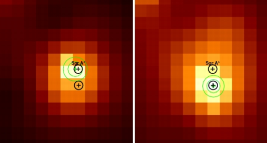
Figure 3.— Smoothed Mos 2 image of the Agust 31 flare with an exposure time of 2000 $\mathrm{s}$ (left panel) and average non-flare image with an exposure of about 50 $\mathrm{ks}$ (right). The boresight corrected position of Sgr A* is labeled and that of CXOGC J174540.0-290031 is marked by a cross. The black circles indicate the 1$\sigma$ uncertainty on the position due to the astrometric correction. The green cross and circles mark the fitted emission centroid and the associated uncertainty at the 68 and 90% confidence levels.

It is evident that the centroid of the emission during the flare is significantly shifted towards Sgr A* and that the transient source CXOGC J174540.0-290031 can be excluded as the flaring source at the 90% confidence level. In the non-flare period, the emission is very closely centered on the transient binary — the central black hole’s closest known, hard X-ray emitting neighboor — and in this case, Sgr A* can be excluded at more than the 90% confidence level as the source of this emission. The error circles on the fitted centroid of the non-flare image are smaller because the statistical uncertainty on the fit is 0${}^{\prime\prime}$ .22 compared with 0${}^{\prime\prime}$ .60 for the flaring source. Combining this value with the same boresight correction uncertainty and rms as was used in the analysis of the flare image yields a total uncertainty of 1${}^{\prime\prime}$ .19.

The first flaring period occurred on 2004 March 31 (Figure 4) and contains one of the two factor-40 flares detected over the course of all four pointings, preceded by two smaller ones. The most prominent flare took place around 23:05 and peaked at 0.76 $\mathrm{cts/s}$ estimated on the basis of 500 $\mathrm{s}$ time bins. This event lasted $\sim$ 2.5 $\mathrm{ks}$ from rise to fall. The PN (black), Mos 1 (red) and Mos 2 (green) spectra for this flare are shown in figure 5.

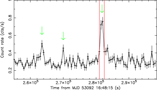
Figure 4.— Zoom on the flare of 2004 March 31 with time bins of 500 $\mathrm{s}$ where the first factor-40 flare occured. Its significance is about 10$\sigma$. The red lines delineate the time window used in the spectral extraction. Two other smaller flares are marked by the green arrows and have significances of abotu 5 and 4$\sigma$ respectively. MJD 53092 corresponds to 2004 March 28.

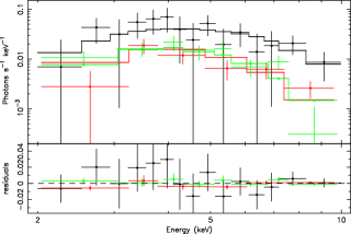
Figure 5.— Epic spectra during the Sgr A* flare of 2004 March 31. The spectra are shown with the best fit absorbed power-law model and the corresponding residuals. The fit is done in the range 2–10 $\mathrm{keV}$. The PN spectrum is shown in black and the Mos  1 and Mos  2 are in red and green respectively.

We fitted each spectrum individually and also simultaneously. The low statistics limits the reliability of the Mos results and for this reason we present the best fit parameters for the PN data as well as for the combined data set in Table 4. Three models were tested: absorbed power-law, black body and bremsstrahlung. All give satisfactory fits. We used the pegpwrlw model in XSpec v 11.3.1 in which the the total unabsorbed flux over the range of the fit is used as the normalization. This allows the photon index and normalization to be fit as independent parameters in the model and to derive the uncertainty on the flux directly from this normalization.

For the pegged power-law model, the best fit values of the combined data set are a photon index of $\Gamma$ = 1.5 $\pm$ 0.5 with a column density of $N_{\rm{H}}$ = (8.3 $\pm$ 2.5) $\times$ $10^{22}$ $\mathrm{cm^{-2}}$. The average unabsorbed flux during the flare was found to be (6.35 $\pm$ 0.45) $\times$ $10^{-12}$ erg cm${}^{-2}$ s${}^{-1}$. Since the count rate at the peak is about twice the average, we estimate that the maximum flux is also about twice the average and so the peak 2–10 $\mathrm{keV}$ luminosity is around 10 $\times$ $10^{34}$ erg s${}^{-1}$ at a distance of 8 $\mathrm{kpc}$; a factor of 45 above quiescence .

The black body was best fit with a temperature of $1.9\pm 0.3$ $\mathrm{keV}$ and absorbing column of $(4.1\pm 1.7)\times 10^{22}~{}\mathrm{cm^{-2}}$. Finally, fitting a bremsstrahlung model resulted in an absorbtion column of $7.8\pm 1.9\times 10^{22}~{}\mathrm{cm^{-2}}$ — similar to that of the power-law — and a temperature around 35 $\mathrm{keV}$. The error range on the temperature, however, is huge and therefore not constraining at all. The large upper bounds in the error of the bremsstrahlung temperature probably reflect the fact that there is no statistically significant break in the spectrum. The best fit parameter values, fluxes and luminosities for the power-law and black-body models are given in Table 4.

The respective occurrence times, peaks and durations of the two small flares that preceded it are: 17:59, 0.51 $\pm$ 0.04 $\mathrm{cts/s}$ ($\sim$ 5$\sigma$) and 1500 $\mathrm{s}$ for the first, and 19:48, 0.45 $\pm$ 0.04 $\mathrm{cts/s}$ ($\sim$ 4$\sigma$) and 1000 $\mathrm{s}$ for the second. These two events are marked by green arrows in Figure 4 Unfortunately, the short duration and lower signal-to-noise ratio of these events prevents us from doing their spectral analysis.

The second major flare was on 2004 August 31 and is shown in detail in Figure 6. The large flare is preceded very closely by what we will call a double-peaked precursor that lasted about the same time as the flare itself. Furthermore, we see a $\sim$ 30% change in flux over about 900 $\mathrm{s}$ or 15 $\mathrm{min}$ between the two peaks of the precursor which constrains the emitting region to less than 2 AU at a distance of 8 $\mathrm{kpc}$. The first peak of the precursor occurred at around 9:00 and the flare that followed rose to its maximum at about 11:05 with a count rate of 0.62 $\pm$ 0.03 $\mathrm{cts/s}$ for 500 $\mathrm{s}$ bins. Both the precursor and the flare lasted $\sim$ 5000 $\mathrm{s}$ and so the whole flaring period had a duration of about 10 000 $\mathrm{s}$ from rise to fall. The narrow peak following the flare occurred at 13:01 and the last flare occurred the next day, 2004 September 1, at 6:48. Figure 7 shows the PN (black), Mos  1 (red), Mos  2 (green) spectra of the flaring event with the best fit absorbed power-law model and residuals.

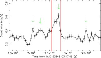
Figure 6.— Light curve of the 2004 August 31 flare binned in 500 $\mathrm{s}$ intervals. Green arrows point out local peaks with respective significances of about 4, 5, 10 and 4$\sigma$. We show the base level of the light curve before and after the flare for reference. The drop in flux at the base of the precursor corresponds to the first of five eclipses in the binary system CXOGC J174540.0-290031 detected during ObsID 866. MJD 53248 corresponds to 2004 August 31.

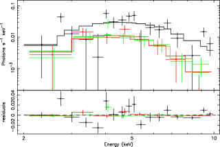
Figure 7.— Epic spectra during the Sgr A* flare of 2004 August 31 fitted in the range 2–10 $\mathrm{keV}$. The colours are the same as in Figure 5.

This flare was modeled in the same way as was done for the March 31 flare and the detailed spectral fitting results are listed in Table 4. The combined spectrum was best fit with an absorbed power-law of photon index $\Gamma$ = 1.9 $\pm$ 0.5 and column density $N_{\rm{H}}$ = (12.5 $\pm$ 3.4) $\times$ $10^{22}$ $\mathrm{cm^{-2}}$. For the black body model, the temperature was 1.8 $\mathrm{keV}$ and the absorbing column density (7.1 $\pm$ 2.3) $\times$ $10^{22}$ $\mathrm{cm^{-2}}$. The bremsstrahlung column density was found to be 11.3 $\pm$ 2.5 with a temperature around 15 $\mathrm{keV}$ but once again the error range is so large that this value cannot be constrained. The low statistics severly limit our ability to detect spectral variations during the flares. The average 2–10 $\mathrm{keV}$ luminosity of this flare is around 4.3 $\times$ $10^{34}$ erg s${}^{-1}$ (see Table 4) and as in the case of the March 31 flare, we estimate the peak luminosity to be about twice the average, and thus reached a maximum intensity around 40 times the quiescent luminosity of Sgr A*.

A summary of the basic temporal features of the two factor-40 flares are given in Table 3. This includes the start, peak and end times of the flares given in UTC and XMM-Newton time in seconds to facilitate reference to the data. We also listed the peak count rate and the deviation from the mean in units of sigma.

Table 3Basic features of X-ray flares

	2004 March 31		2004 August 31
	UTC	XMM time (s)	UTC	XMM time (s)
Start time	22:48	1.9716050+08	09:58	2.1033350+08
Peak time	23:09	1.9716175+08	11:05	2.1033750+08
End time	23:22	1.9716250+08	11:22	2.1033850+08
Duration (s)	2 500		5 000
Peak rate (cts/s)	$0.760\pm 0.048$		$0.617\pm 0.035$
Mean rate (cts/s)	$0.303\pm 0.002$		$0.293\pm 0.002$
Deviation ($\sigma$)	9.6		9.7

Note. — Error bars correspond to the 68$\%$ confidence interval. Count rates and times are estimated using 500 $\mathrm{s}$ time bins.

3.2. Timing Analysis

The cyclical decrease in flux observed during ObsID 866 (first portion of Figure 2) occurs with a period of about 8 $\mathrm{h}$ and is most probably due to an eclipse in the binary system CXOGC J174540.0-290031. A complete analysis of the XMM-Newton obsevations of this transient source are presented by Porquet et al. (2005), and the results of the Chandra observations by Muno et al. (2005b).

A spectral density analysis of the X-ray data from Sgr A* was performed and since XMM-Newton’s spatial resolution severely limits our ability to distinguish the quiescent emission of Sgr A* from that of its surroundings, temporal structures in the X-rays emission detected by XMM-Newton from the Galactic center can only be attributed to Sgr A* with confidence if seen during a flare, when the flux rises substantially above the quiescent emission. Therefore, periodic features seen in the base level of the light curve cannot readily be attributed to Sgr A*. Furthermore, a period detected during a flare can only be confidently attributed to Sgr A* if it is not present in the rest of the light curve.

Since the range of frequencies and resolution in a periodogram are primarily functions of the total length of the observation and sampling or bin time, only the second of the two factor-40 flares allowed us to perform a meaningful search for periodic modulations. This event lasted about 10 $\mathrm{ks}$ including the precursor. This is about 4 times longer than the first.

The first analysis revealed a periodic structure that could be significant but the proper treatment of the signal that includes white and possibly a component of red noise, requires a detailed analysis that is quite complex and that we have begun but will present elsewhere upon completion.

4. Discussion and Conclusion

We observed the neighborhood of Sgr A* for more than three consecutive days from 2004 March 28 to April 1, and an additional three consecutive days from 2004 August 31 to September 3. Both observations were interrupted for only $\approx 30$ $\mathrm{ks}$ and during each of these observation periods we detected flaring activity composed in each case of a large flare accompanied by smaller ones. The two main flares are positionally coincident with Sgr A* and, as Baganoff et al. (2001), we associate these with the supermassive black hole at the center of the Milky Way, given our current knowledge of the region surrounding this source. These flares, both with peak luminosities about 40 times that of the assumed quiescent level, exhibit similar spectral characteristics: a hard photon index of $\Gamma$ $\approx$ 1.5–1.9 and a column density $N_{\rm H}$ $\approx$ 8–13 $\times$ $10^{22}$ $\mathrm{cm^{-2}}$. These parameter values are more akin to those of the first two detected flares (Baganoff et al. 2001; Goldwurm et al. 2003), than to those of the very bright flare reported by Porquet et al. (2003).

There were a total of three flares with significance greater than 3$\sigma$, corresponding to a factor of 15 above Sgr A*’s quiescent level in ObsID 789 and the same number in ObsID 866, if we consider the precursor to be a separate flaring event. Although we cannot determine the position of the smaller flares accurately and thus cannot attribute them to Sgr A* with certainty, if these are indeed coming from the central black hole then, irrespective of the temporal distribution of these flares, our estimate of their average occurrence rate is about 1 per day. This estimate agrees with those based on Chandra observations performed between 1999 and 2002 (Baganoff 2003b, ). Note that flares from Sgr A* appear to occur in clusters.

In light of the recently detected near-IR spectrum of Sgr A* (Genzel et al. , 2003), and of the constraints that it imposes on the various emission models for this source, the flares we detected could have resulted from a sudden increase in accretion accompanied by a reduction in the anomalous viscosity, which would point to thermal bremsstrahlung as the X-ray emission process. This would give rise to a hard spectrum, unlike the softer one expected from a synchrotron self-Compton process (Liu & Melia 2002a, ).

Another possibility is that the flares arose from the quick acceleration of electrons in the accretion flow near the black hole, producing either a two-component distribution characterized by a broken power-law, with steep low-energy and flat high-energy components, or a modified thermal distribution with a high-energy enhancement (see, e.g. Liu, Petrosian, & Melia 2004; Yuan, Quataert, & Narayan 2003 and 2004). In either of these cases, the lower energy electrons produce the near-IR emission and the high-energy distribution produces the hard X-rays. Further, the rather short time scale ($\sim$ 2500–4500 $\mathrm{s}$) and hard spectral index ($\Gamma$ = 1.6) of the flares would, according to this model, favor magnetic reconnection as the engine of the event.

In either of these two scenarios — an accretion instability, or a magnetic reconnection event — one could expect to see a modulation in the light curve, mirroring the underlying Keplerian period of the emitting plasma. Indications of the presence of such a periodic modulation during a near-IR flare were presented by Genzel et al. (2004) and during an X-ray flare by Ascenbach et al. (2002). These results must be confirmed by similar detections in other events seen in the near-IR and X-ray bands. A search for such a semi-periodic modulation in the longer of the two factor-40 flares from Sgr A* presented here is under way and the results will be reported elsewhere.

The accretion instability scenario predicts a strong correlation between the sub-mm/IR and the X-ray photons with no or little change in the millimeter flux density. The two-component synchrotron model predicts possible, though not necessary, correlations between X-ray and near-IR flares, with larger X-ray amplitudes in the case of simultaneous flaring, important variations in the spectral slopes of the X-ray flares compared with those in the near-IR flares, and small amplitude variability in the radio and sub-millimeter wavebands. It is on this last point that we could distinguish the accretion induced X-ray flare model from the two-component synchrotron model.

Table 4Spectral Characteristics of X-ray Flares

	Power-law						Black Body
			$F_{\rm{X}}$[2–10]							$F_{\rm{X}}$[2–10]
	$N_{\rm{H}}$		($10^{-12}$ erg	$L_{\rm{X}}$[2–10]			$N_{\rm{H}}$	kT	Norm	($10^{-12}$ erg	$L_{\rm{X}}$[2–10]
Date (Instr.)	($10^{22}$ $\mathrm{cm^{-2}}$)	$\Gamma$	cm${}^{-2}$ s${}^{-1}$)	($10^{34}$ erg s${}^{-1}$)	C/bins		($10^{22}$ $\mathrm{cm^{-2}}$)	(keV)	($10^{-5}$)	cm${}^{-2}$ s${}^{-1}$)	($10^{34}$ erg s${}^{-1}$)	C/bins
March 31 (PN)	$8.0^{+3.3}_{-2.8}$	$1.7^{+0.6}_{-0.6}$	$4.0^{+0.4}_{-0.9}$	$5.1^{+0.3}_{-0.7}$	689/740		$3.4^{+2.3}_{-1.9}$	$1.9^{+0.5}_{-0.3}$	$7.4^{+1.6}_{-1.2}$	$4.0^{+1.2}_{-1.6}$	$3.6^{+0.7}_{-1.4}$	691/740
March 31 (All)	$8.3^{+2.5}_{-2.1}$	$1.5^{+0.5}_{-0.4}$	$4.0^{+0.3}_{-0.4}$	$4.9^{+0.9}_{-0.7}$	883/936		$4.1^{+1.7}_{-1.5}$	$1.9^{+0.2}_{-0.3}$	$7.4^{+1.6}_{-0.8}$	$3.8^{+0.7}_{-0.9}$	$4.6^{+0.5}_{-0.9}$	886/936
August 31 (PN)	$10.0^{+3.4}_{-2.5}$	$1.3^{+0.5}_{-0.5}$	$2.7^{+0.2}_{-0.4}$	$3.4^{+0.8}_{-0.5}$	883/731		$6.5^{+2.3}_{-1.7}$	$2.1^{+0.4}_{-0.3}$	$5.9^{+1.5}_{-0.8}$	$2.6^{+0.5}_{-0.9}$	$2.6^{+0.4}_{-0.8}$	883/731
August 31 (All)	$12.5^{+3.4}_{-2.8}$	$1.9^{+0.5}_{-0.5}$	$2.7^{+0.2}_{-0.4}$	$4.3^{+1.2}_{-0.8}$	1082/913		$7.1^{+2.3}_{-2.1}$	$1.8^{+0.3}_{-0.2}$	$5.7^{+0.9}_{-0.5}$	$2.6^{+0.4}_{-0.4}$	$2.9^{+0.3}_{-0.7}$	1086/913

Note. — Errors on fitted parameters correspond to the 68$\%$ confidence interval. Flux density for the Power-law model is normalized over the range from 2 to 10 keV and corresponds to the total unabsorbed flux in this range. The listed flux values are absorbed with the associated column density and the luminosity is calculated using the power-law normalization and is derived for a distance of 8 $\mathrm{kpc}$ to the Galactic center. In the Black Body model, the normalization corresponds to the dimensionless ratio of the luminosity in units of $10^{39}$ erg s${}^{-1}$ to the distance in units of 10 $\mathrm{kpc}$ squared. In the first column, ’Instr.’ refers to the instrument whose data was used in the fit and ’All’ refers to the combination of PN, Mos 1 and Mos 2.

References

- Baganoff et al. (2001) Baganoff, F. K. et al. 2001, Nature, 413, 45
- Baganoff et al. (2003) Baganoff, F. K. et al. 2003, ApJ, 591, 891
- (3) Baganoff, F. K. 2003, AAS/High Energy Astrophysics Division, 7
- Bélanger et al. (2005) Bélanger, G. et al. 2005, ApJ, in press
- Bower et al. (2005) Bower, G. et al. 2005, ApJ, in press (astro-ph/0507221)
- Eckart et al. (2004) Eckart, A., et al. 2004, A&A, 427, 1
- Genzel et al. (2003) Genzel, R. et al. 2003, Nature, 425, 934
- Ghez et al. (2003) Ghez, A. M., et al. 2003, ApJ, 586, L127
- Goldwurm et al. (2003) Goldwurm, A. et al. 2003a, ApJ, 584, 751
- Hog et al. (2000) Hog, E., et al. 2000, A&A, 363, 385
- Liu & Melia (2001) Liu, S. & Melia, F. 2001, ApJ, 561, L77
- (12) Liu, S. & Melia, F. 2002a, ApJ, 566, L77
- (13) Liu, S. & Melia, F. 2002b, ApJ, 573, L23
- Liu, Petrosian & Melia (2004) Liu, S., Petrosian, V. & Melia, F. 2003, ApJ, 611, L101
- Kirsch (2005) Kirsch, M. 2005, XMM-SOC-CAL-TN-0018
- Markoff et al. (2001) Markoff, S. et al. 2001, A&A, 379, L13
- Melia et al. (2001) Melia et al. 2001, ApJ, 554, L37
- Melia & Falcke (2001) Melia, F. & Falcke, H. 2001, ARA&A, 39, 309
- (19) Muno, M. et al. 2003a, ApJ, 589, 225
- (20) Muno, M. et al. 2005a, ApJ, in press (astro-ph/0412492)
- Porquet et al. (2003) Porquet, D. et al. 2003, A&A, 407, L17
- Porquet et al. (2005) Porquet, D. et al. 2005, A&A, in press
- Schödel et al. (2003) Schödel, R. et al. 2003, ApJ, 596, 1015
- Yuan, Quataert, & Narayan (2003) Yuan, F., Quataert, E., & Narayan, R. 2003, ApJ, 598, 301
- Yuan, Quataert, & Narayan (2004) Yuan, F., Quataert, E., & Narayan, R. 2004, ApJ, 606, 894
- Yusef-Zadeh et al. (1999) Yusef-Zadeh, F., Choate, D. & Cotton, W. 1999, ApJ, 518, L33
- Zhao et al. (2001) Zhao, J.-H., Bower, G. C., & Goss, W. M. 2001, ApJ, 547, L29