Effect of the radiative background flux in convection

Abstract

Numerical simulations of turbulent stratified convection are used to study models with approximately the same convective flux, but different radiative fluxes. As the radiative flux is decreased, for constant convective flux: the entropy jump at the top of the convection zone becomes steeper, the temperature fluctuations increase and the velocity fluctuations decrease in magnitude, and the distance that low entropy fluid from the surface can penetrate increases. Velocity and temperature fluctuations follow mixing length scaling laws.

1 Introduction

In modeling stellar convection it is important to make the models resemble the stars as much as possible. A major difficulty in producing realistic simulations of deep stellar convection is the large ratio between thermal and dynamical time scales. This is because in dynamical units the solar thermal flux ($F_{\odot}=7\times 10^{10}\,{\rm erg}\,{\rm cm}^{-2}\,{\rm s}^{-1}$) is very small,

$${F_{\odot}\over\rho c_{\rm s}^{3}}\sim 4\times 10^{-11},$$ (1)

at the bottom of the convection zone (where $\rho=0.2\,{\rm g}\,{\rm cm}^{-3}$ and $c_{\rm s}=200\,{\rm km/s}$). At the surface this ratio is of order $10^{-1}$, but already two megameters below the surface the ratio is $10^{-3}$. This ratio is basically equal to the ratio of the dynamical to thermal time scales.

For a common class of models studied by many workers (we will refer to them as polytropic models), most of the energy is carried by radiation instead of convection. This corresponds to the polytropic index $m$ of the associated hydro-thermal equilibrium solution having the value $m=1$. In this case flow characteristics are different from those in the convection dominated transport regime, even for large Rayleigh numbers. In the range $-1<m\ll 1$, however, most of the flux is carried by convection.

In order for simulations of convection to be representative of late type stars the ratio of radiative to total flux must be small in the convection zone. This has prompted Chan & Sofia (1986, 1989) to study models where the radiative flux is removed entirely and is replaced by a subgrid scale flux. Unlike the radiative flux, which is proportional to the temperature gradient, the subgrid scale or small-scale eddy flux is proportional to the entropy gradient (e.g. Rüdiger 1989). Others have chosen to model the surface layers and the granulation (Nordlund 1982; Stein & Nordlund 1989, 1998; Kim & Chan 1998, Robinson et al. 2003, Vögler et al. 2005). In those models radiation is only important near the surface layers and practically absent beneath the surface, although diffusive energy flux is still necessary for numerical simulations to be stable.

The aim of this paper is to explore the effect of varying the diffusive radiative flux while keeping the convective flux in the convection zone approximately constant. From mixing length arguments one would expect that for negligible radiative flux the turbulent velocities, temperature fluctuations and other dynamical aspects of the convection only depend on the magnitude of the convective flux. However, this approximation breaks down once the radiative flux is no longer very small compared to the convective flux.

We consider models using piecewise polytropic layers. Such models have been widely studied and they possess the advantage that the properties of stable and unstable layers are easier to manipulate than in models with the more realistic Kramers’ opacities, for example, where the radiative diffusivity depends on density and temperature rather than just on depth. However, we also include a comparison of realistic solar models with the same convective flux but varying diffusive subgrid scale energy flux in the interior and hence varying (turbulent) Prandtl number.

There are two main results of our investigation. First, the properties of the convection depend on the ratio of radiative to convective flux when the radiative flux is not negligible. Increasing radiative energy diffusion reduces the temperature fluctuations which requires larger velocities to carry the same convective flux. Increasing radiative energy diffusion also raises the entropy of the downdrafts and inhibits their descent. Second, as the resolution increases the dependence of convective properties on the Prandtl number decreases. However, at low resolutions the dependence is different when the viscosity is altered than when the radiative conductivity is altered. Increasing the radiative conductivity to lower the Prandtl number has the effects described above. Decreasing the viscosity to lower the Prandtl number (increasing the Reynolds number) enhances small scale structures and increases the turbulence.

We first discuss the setup of our model, the equations that are solved and how we change the fractional radiative flux in the convection zone while leaving everything else unchanged (Sec. 2). The polytropic model results are given in Sects 3 and 4, the realistic solar simulation results are presented in Sec. 5, and our conclusions are given in Sec. 6.

2 The model

2.1 Equations

In our polytropic models we solve the continuity, momentum, and energy equations in non-conservative form,

$${D\ln\rho\over Dt}=-\mbox{\boldmath$\nabla$}{}\cdot\mbox{\boldmath$u$}{},$$ (2)

$${D\mbox{\boldmath$u$}{}\over Dt}=-(\gamma-1)\,(e\mbox{\boldmath$\nabla$}{}\ln\rho+\mbox{\boldmath$\nabla$}{}e)+\mbox{\boldmath$g$}{}+{1\over\rho}\mbox{\boldmath$\nabla$}{}\cdot(2\nu\rho\mbox{\boldmath${\sf S}$}{}),$$ (3)

$${De\over Dt}=-(\gamma-1)\,e\mbox{\boldmath$\nabla$}{}\cdot\mbox{\boldmath$u$}{}+{1\over\rho}\mbox{\boldmath$\nabla$}{}\cdot{K}\mbox{\boldmath$\nabla$}{}T+2\nu\mbox{\boldmath${\sf S}$}{}^{2}-{e-e_{0}\over\tau_{e}(z)},$$ (4)

where ${\sf S}_{ij}={\textstyle{1\over 2}}(\partial_{j}u_{i}+\partial_{i}u_{j}-{\textstyle{2\over 3}}\delta_{ij}\partial_{k}u_{k})$ is the (traceless) strain tensor, $\nu=\mbox{const}$ is the kinematic viscosity. We assume a perfect gas, so the pressure is given by

$$p=(\gamma-1)\rho e,$$ (5)

where $\rho$ is density, $e=c_{\rm v}T$ is the internal energy, $T$ is temperature, and $c_{\rm v}$ is the specific heat at constant volume.

Below the photosphere the radiative diffusion approximation is valid so the vertical component of the radiative flux is

$$F_{\rm rad}=KdT/dz,$$ (6)

where $K$ is the radiative conductivity, $T$ is temperature, and $z$ is depth (increasing downward). We impose a cooling layer at the surface where $\tau_{e}(z)$ is a cooling time, and $e_{0}$ is the reference value of the internal energy $e$ at the top of the layer. The value of $e_{0}$ is quantified by a parameter $\xi_{0}=(\gamma-1)e_{0}/(gd)\equiv H_{p}^{\rm(top)}/d$, which is the pressure scale height at the top of the box divided by the depth of the unstable layer, $d$. The pressure scale height is, $H_{p}=(d\ln p/dz)^{-1}={\cal R}T/(\mu g)$, where ${\cal R}$ is the universal gas constant and $\mu$ the mean molecular weight.

We adopt the basic setup of the model of Brandenburg et al. (1996, hereafter BJNRST; see also Hurlburt et al. 1986) where the vertical profile of ${\cal K}(z)\equiv K/c_{\rm v}$ is assumed such that ${\cal K}$ is piecewise constant in three different layers, ${\cal K}={\cal K}_{1}$ in $z_{1}\leq z\leq z_{2}$, ${\cal K}={\cal K}_{2}$ in $z_{2}\leq z\leq z_{3}$, and ${\cal K}={\cal K}_{3}$ in $z_{3}\leq z\leq z_{4}$. In our case $z_{1}=-0.15$, $z_{2}=0$, $z_{3}=1$, and $z_{4}=2.8$.

2.2 Radiative conductivity

In this paper we want to study the effects of varying the radiative flux in the convection zone, $z_{2}\leq z\leq z_{3}$, so we have to vary the value of ${\cal K}_{2}$. In the following we discuss the relation between ${\cal K}_{2}$ and the anticipated radiative flux $F_{\rm rad}$ in the convection zone, which will be a good approximation to the actual radiative flux obtained by solving Eqs. (2)–(4).

In astrophysics the radiative flux is often written in the form

$$F_{\rm rad}=KT\,\left({d\ln p\over dz}\right)\,\left({d\ln T\over d\ln p}\right)={KT\over H_{p}}\,\nabla={Kg\over{\cal R}/\mu}\,\nabla.$$ (7)

Here

$$\nabla=d\ln T/d\ln p$$ (8)

characterizes the temperature stratification. We can define a radiative gradient, $\nabla_{\rm rad}$, that would be necessary to transport all the flux radiatively,

$$F_{\rm tot}={Kg\over{\cal R}/\mu}\,\nabla_{\rm rad}.$$ (9)

In the deep radiative interior of the sun we have $F_{\rm rad}=F_{\rm tot}$, and therefore $\nabla=\nabla_{\rm rad}$. In most of the convection zone the actual stratification is close to adiabatic, so $\nabla\approx\nabla_{\rm ad}\equiv 1-\gamma^{-1}<\nabla_{\rm rad}$, since $F_{\rm rad}<F_{\rm tot}$.

To set up a polytropic model it is customary to specify ${\cal K}$ in terms of the polytropic index $m$ (e.g., Hurlburt & Toomre 1984), instead of $\nabla_{\rm rad}$. If all the flux were carried by radiation we would have $p(z)\sim T^{m+1}$, and so $\nabla_{\rm rad}=(m+1)^{-1}$. The value of the radiative conductivity is expressed in terms of the polytropic index from Eq. (9) as

$${\cal K}_{i}={K_{i}\over{c_{v}}}={F_{\rm tot}\over g}\,(\gamma-1)(m_{i}+1).$$ (10)

The three values of ${\cal K}_{i}$ ($i=1,2,3$) are given in terms of polytropic indices $m_{i}$ via the above equation. In all cases reported below we use $m_{3}=3$ and vary the value of $m_{2}$. Near the top there is cooling ($\tau_{e}\neq 0$ in $z_{1}<z<z_{2}$, and $\tau_{e}\rightarrow 0$ for $z>z_{2}$). Therefore, almost all the flux in this layer is transported by the corresponding cooling flux and the diffusive radiative flux in the uppermost layer is insignificant. Hence, the value of $m_{1}$ does not affect the stratification. In most of the cases we put $m_{1}=-0.9$.

The fractional radiative flux in the convection zone is

$${F_{\rm rad}\over F_{\rm tot}}\approx{\nabla_{\rm ad}\over\nabla_{\rm rad}}=\left(1-{1\over\gamma}\right)(m+1),\;\;\mbox{for}\;\;m<{1\over\gamma-1},$$ (11)

where we have assumed $\nabla\approx\nabla_{\rm ad}$. In all those models where $m=1$ (e.g. Hurlburt & Toomre 1984, 1986; Cattaneo et al. 1990, 1991; Brandenburg et al. 1990, 1996; Brummell et al. 1996, Ossendrijver et al. 2002, Ziegler & Rüdiger 2003, Käpylä et al. 2004) and $\gamma=5/3$, the fractional radiative flux is as large as 80%. In order to study polytropic models with $F_{\rm rad}\ll F_{\rm tot}$ we must approach the limit $m\rightarrow-1$. In this paper we calculate a series of such models starting with $m=1$ (the standard case considered in many papers) down to $m=-0.9$. As the value of $m$ is lowered, smaller fractional radiative fluxes are obtained. In the upper layers of the solar convection zone this ratio is close to the ratio of the mean free path of the photons to the pressure scale height and can be as small as $10^{-5}$. In deeper layers of the solar convection zone the radiative flux becomes progressively more important and reaches 50% of the total flux at 0.75 solar radii.

It may seem unphysical to talk about negative values of $m$, because the density would increase with height, but such a ‘top-heavy’ arrangement only means that the stratification is then very unstable. Of course, the pressure still decreases with height, because $m+1$ is positive. Negative values of $m$ (but with $m>-1$) result from a very poor radiative conductivity, which is indeed quite common in the outer layers of all late-type stars.

It should be emphasized that $m$ only characterizes the associated thermal equilibrium hydrostatic solution, which is of course unstable for $m<m_{\rm ad}\equiv(\gamma-1)^{-1}=3/2$. In that case convection develops, making the stratification close to adiabatic. Thus, the effective value of $m$ will then always be close to the marginal value $m_{\rm ad}$. The significance of the $m$ used here (as opposed to the effective $m$) is that it gives a nondimensional measure of the fractional radiative flux.

We carry out a parameter survey by varying the values of $m_{2}$ and hence ${\cal K_{2}}$, which corresponds to varying $\nabla_{\rm rad}$ in the convection zone and the total flux $F_{\rm tot}$. In practice we fix the value of ${F}_{\rm conv}$ and calculate the total flux ${F}$ from ${F}_{\rm conv}$ for a given value of $m_{2}$. In Table LABEL:Tfluxes we give the fractional fluxes for some values of $m$, using Eq. (11). Here we have assumed $F_{\rm tot}=F_{\rm rad}+F_{\rm conv}$, i.e. we have neglected kinetic and viscous fluxes which are of course included in the simulations.

Table 1: Fractional radiative and convective fluxes for a few values of $m$, as obtained from Eq. (11).

$m$ $F_{\rm rad}/F_{\rm tot}$ $F_{\rm conv}/F_{\rm tot}$ $1$ 80% 20% $0$ 40% 60% $-0.5$ 20% 80% $-0.8$ 8% 92% $-0.9$ 4% 96%

2.3 Nondimensional quantities

Nondimensional quantities are adopted by measuring length in units of $d$, time in units of $\sqrt{d/g}$ and $\rho$ in units of its initial value, $\rho_{0}$, at $z=z_{3}$, i.e. at the bottom of the convection zone. In all cases we use a box size of $L_{x}=L_{y}=4$ with $z_{4}=2.8$. The flux is then expressed in terms of the non-dimensional quantity

$${\cal F}={F_{\rm tot}\over\rho_{0}\,(gd)^{3/2}},$$ (12)

In the same units we define

$${\cal F}_{\rm conv}=\left[1-\left(1-{1\over\gamma}\right)(m+1)\right]{\cal F},$$ (13)

which is a measure of the convective flux. (The actual convective flux, $F_{\rm conv}$, is of course not a constant, but varies with height, and reaches a maximum of around ${\cal F}_{\rm conv}$.)

The value of $\nu$ is taken to be as small as possible for a given mesh resolution. For $50^{3}$ we can typically use $\nu=5\times 10^{-3}$ (in units of $\sqrt{gd^{3}}$). For a resolution of $200^{3}$ we were able to lower the viscosity to $\nu=2.4\times 10^{-4}$.

The quantity ${\cal F}$ determines the ‘mean’ thermal diffusivity, $\overline{\chi}_{3}={\cal K}_{3}/(\gamma\rho_{0})$, via

$$\overline{\chi}_{i}=\sqrt{gd^{3}}\,{\cal F}\,\nabla_{\rm ad}/\nabla_{\rm rad}^{(i)},$$ (14)

where $\nabla_{\rm rad}^{(i)}$ is the radiative gradient in layer $i$. (Note that in this approach the actual thermal diffusivity decreases with depth in each of the three layers.) The nondimensional flux can also be related to the Rayleigh number,

$$\mbox{Ra}={gd^{4}\over\nu\overline{\chi}_{2}c_{p}}\left({ds\over dz}\right)_{0},$$ (15)

which characterizes the degree of instability of the hydrostatic solution in the middle of the unstable layer, $i=2$. Here,

$${d\over c_{p}}\left({ds\over dz}\right)_{0}={1-\nabla_{\rm ad}/\nabla_{\rm rad}^{(2)}\over{\textstyle{1\over 2}}+\xi_{0}/\nabla_{\rm rad}^{(2)}}$$ (16)

is the normalized entropy gradient of the associated hydrostatic solution for the same ${\cal K}(z)$ profile (see BJNRST). We can then express Ra in terms of ${\cal F}$ as

$$\mbox{Ra}={1\over\mbox{Pr}\,{\cal F}^{2}}\,\left({\nabla_{\rm rad}^{(2)}\over\nabla_{\rm ad}}\right)^{2}{1-\nabla_{\rm ad}/\nabla_{\rm rad}^{(2)}\over{\textstyle{1\over 2}}+\xi_{0}/\nabla_{\rm rad}^{(2)}},$$ (17)

where $\mbox{Pr}=\nu/\overline{\chi}_{2}$ is the Prandtl number. In the astrophysically interesting limit, $\nabla_{\rm rad}^{(2)}\rightarrow\infty$, we have

$$\mbox{Ra}\rightarrow\mbox{Ra}^{*}=2\mbox{Pr}^{-1}\,{\cal F}^{-2}\,(\nabla_{\rm rad}^{(2)}/\nabla_{\rm ad})^{2},$$ (18)

so large Rayleigh numbers correspond to small normalized fluxes and hence small velocities. This is at first glance somewhat surprising, because large Rayleigh numbers are normally associated with more vigorous convection and therefore large velocities. However, while the velocity decreases in absolute units, it does increase relative to viscosity and radiative diffusivity, i.e. the Reynolds and Peclet numbers do indeed increase.

2.4 The initial condition

The ratio of radiative to convective flux can easily be decreased within the framework of standard polytropic models, provided the polytropic index $m$ is close to $-1$. In that case, however, it is a bad idea to use the corresponding polytropic solution as the initial condition, because it is extremely far away from the final solution and would take a very long time to relax to the final state. Instead, we use a simplified mixing length model with an empirically determined free parameter such that the entropy at the bottom of the convection zone and the radiative interior beneath is close to that finally obtained in the actual simulation.

An initial condition that yields a solution on almost the right adiabat is obtained by assuming that the entropy is not constant, but that the negative entropy gradient is a function of the convective heat flux. According to mixing length theory the superadiabatic gradient in the convection zone is

$$\nabla-\nabla_{\rm ad}=k\,({F_{\rm conv}/\rho c_{\rm s}^{3}})^{2/3},$$ (19)

where $k$ is a nondimensional coefficient (related to the mixing length alpha parameter), which we determined empirically for our models to be $k=1.5$.

In terms of $e$ and $\ln\rho$, our initial condition can then be written as

$$de/dz=m_{\rm ad}g\,\nabla,$$ (20)

$$d\ln\rho/dz=m_{\rm ad}g\,(1-\nabla)/e,$$ (21)

where

$$\nabla=\left\{\begin{array}[]{ll}0&\quad\mbox{if}\quad z_{1}\leq z\leq z_{2}\\ \nabla_{\rm ad}+k\,({F_{\rm conv}/\rho c_{\rm s}^{3}})^{2/3}&\quad\mbox{if}\quad z_{2}<z<z_{3}\\ \nabla_{\rm rad}^{(3)}=(m_{3}+1)^{-1}&\quad\mbox{if}\quad z_{3}\leq z\leq z_{4}\end{array}\right.$$ (25)

and varies smoothly between the three layers. The initial stratification is obtained by integrating Eqs (20) and (21) from $z=z_{1}$ downwards to $z_{4}$. The starting value of $\rho$ at $z=z_{1}$ is adjusted iteratively such that $\rho(z_{3})=\rho_{0}=1$, i.e. the density at the bottom of the convection zone is unity. This is especially useful if the extent of the box is changed, because this would otherwise affect the density in all layers.

In Fig. 1 we compare the entropy obtained from the initial condition as derived above with that obtained from the actual simulations. We also compare with the entropy derived from the associated polytropic hydrostatic thermal equilibrium solution to show just how far away from the final state that solution would be. Finally, we also compare with a solution where the entropy was assumed constant within the convection zone, which is better than the associated hydrostatic thermal equilibrium, but still with the wrong entropy at the bottom of the convection zone.

Figure 1: Entropy in the final and initial states, compared with the corresponding polytropic model, as well as a polytropic model with constant entropy within the convection zone (CZ). ${\cal F}_{\rm conv}=0.01$.

As in previous work the initial velocity is random. This is realized by a superposition of randomly located spherical blobs of radius 0.1, where the velocity points in random directions.

2.5 Boundary conditions

In the horizontal directions we adopt periodic boundary conditions and at the top and bottom we adopt impenetrable, stress-free boundary conditions, i.e.

$${\partial u_{x}\over\partial z}={\partial u_{y}\over\partial z}=u_{z}=0\quad\mbox{at}\quad z=z_{1},z_{4}.$$ (26)

The boundaries are sufficiently far away so the boundary conditions do not significantly affect the flow properties in the convection zone proper, which is the layer $z_{2}\leq z\leq z_{3}$. Because of the cooling term in Eq. (4) the value of $e$ at the top is always close to the reference value $e_{0}$ which, in turn, is proportional to $\xi_{0}$ and to the pressure scale height at the top. Thus, decreasing the value of $\xi_{0}$ leads to stronger driving of convection and to stronger stratification in the top layer. However, $\xi_{0}$ cannot be decreased too much for a given numerical resolution, and so we chose $\xi_{0}=0.2$ in all cases. In the top layer $z_{1}<z<z_{2}$ the inverse cooling time $\tau_{e}^{-1}$ is 10 and goes smoothly to zero for $z>z_{2}$.

3 Results

3.1 Models

We have carried out a series of calculations all with the same value of ${\cal F}_{\rm conv}$ and varying values of $m_{2}$ (hereafter referred to as $m$). In a first series of models we used $\nu=6\times 10^{-3}$. The corresponding values of Prandtl and Rayleigh numbers are given in Table LABEL:Tfluxes2.

Table 2: Parameters for a model with ${\cal F}_{\rm conv}=0.01$, $\xi_{0}=0.2$, $\nu=6\times 10^{-3}$ and different values of $m$.

$m$ ${\cal F}_{\rm tot}$ ${\cal F}_{\rm rad}$ Pr Ra $1$ 0.0500 0.0400 0.15 $9.3\times 10^{2}$ $0$ 0.0167 0.0067 0.9 $2.1\times 10^{4}$ $-0.5$ 0.0125 0.0025 2.4 $8.9\times 10^{4}$ $-0.8$ 0.0109 0.0009 6.9 $3.3\times 10^{5}$ $-0.9$ 0.0104 0.0004 14 $7.4\times 10^{5}$

Note that the Prandtl number is no longer small, except in the case $m=1$. However, for $m=1$ and ${\cal F}_{\rm conv}=0.01$ the Rayleigh number is already so small that the instability to convection is suppressed. Therefore we have also studied another series of models where the convective flux is reduced by a factor of 5; see Table LABEL:Tfluxes3. Here however we have only calculated the cases $m=0$ and 1, because otherwise the radiative diffusivity would become so small that the resolution would be insufficient.

Table 3: Parameters for a model with ${\cal F}_{\rm conv}=0.002$ and $\nu=5\times 10^{-3}$ and different values of $m$.

$m$ ${\cal F}_{\rm tot}$ ${\cal F}_{\rm rad}$ Pr Ra $1.0$ 0.01000 0.00800 0.6 $5.6\times 10^{3}$ $0.0$ 0.00333 0.00133 3.8 $1.3\times 10^{5}$

Finally, we consider a series of models with varying Prandtl number and constant convective flux. Lowering the radiative flux automatically increases the Prandtl number. In the sun the Prandtl number is less than one, which was no longer the case in models with low radiative flux. We therefore also studied the effects of lowering the Prandtl number by lowering the viscosity. In Table LABEL:Tfluxes4 we give the parameters for a series of models where Pr is varied by changing both $\nu$ and $\overline{\chi}_{2}$. The question is whether or not certain properties of convection continue to depend on Prandtl number as the turbulence becomes more vigorous (small viscosity and radiative diffusivity). For instance, we expect that for sufficiently large Reynolds number the large scale flow properties will no longer depend on the microscopic values of viscosity and radiative diffusivity.

Table 4: Parameters for a model with ${\cal F}_{\rm conv}=0.01$ and different values of $m$. $\nu$ and $\overline{\chi}_{2}$ are given in units of $10^{-4}$, i.e. $\nu_{-4}=\nu/10^{-4}$ and $\chi_{-4}=\overline{\chi}_{2}/10^{-4}$. The mesh resolution is also given. The asterisk in the last column indicates that the duration of the run was short and not yet fully relaxed, so the data may not be reliable.

$m$ $\nu_{-4}$ $\chi_{-4}$ Pr Ra resol. $k_{u}$ $k_{T}$ $-0.5$ 60 25 2.4 $9\times 10^{4}$ $50^{3}$ 0.34 1.13 $-0.5$ 12 25 0.5 $4\times 10^{5}$ $100^{3}$ 0.46 1.07 $-0.9$ 60 4 14 $7\times 10^{5}$ $100^{3}$ 0.29 1.25 $-0.9$ 12 4 2.9 $4\times 10^{6}$ $100^{3}$ 0.41 1.14 $-0.9$ 2.4 4 0.6 $2\times 10^{7}$ $200^{3}$ 0.48 1.14 * $-.98$ 12 0.8 15 $2\times 10^{7}$ $100^{3}$ 0.38 1.22 $-.98$ 2.4 0.8 3.0 $1\times 10^{8}$ $200^{3}$ 0.43 1.16

3.2 Entropy stratification

As the radiative flux is lowered, the mean entropy in the convection zone becomes more nearly constant and the superadiabatic gradient at the top becomes steeper; see Fig. 2. The mean entropy beneath the convection zone is only slightly affected.

Figure 2: Comparison of the horizontally averaged entropy stratification for different values of $m$ and ${\cal F}_{\rm conv}=0.01$.

Figure 3: Entropy histograms for different values of $m$ and ${\cal F}_{\rm conv}=0.01$ at three different values of $z$.

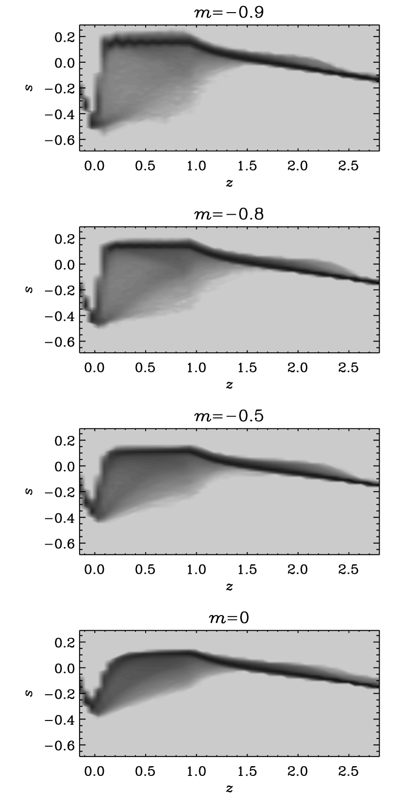
Figure 4: Entropy histograms for different values of $m$ and ${\cal F}_{\rm conv}=0.01$.

As the radiative flux decreases the minimum entropy in the interior of the convection zone decreases (Fig. 3 and Fig. 4) and approaches the minimum value that occurs at the top of the convection zone. These low entropy elements are only produced at the top where cooling is important. As the diffusive energy exchange decreases at least some fluid elements make it all the way from the top to the bottom with very little mixing or heating. This is clearly a consequence of the reduced radiative diffusivity in the cases with low radiative flux. In the case $m=1$ the deviations from the median of the entropy are rather small; see Fig. 5, where ${\cal F}_{\rm conv}=0.002$ instead of ${\cal F}_{\rm conv}=0.01$, so the entropy drop at the surface is obviously smaller.

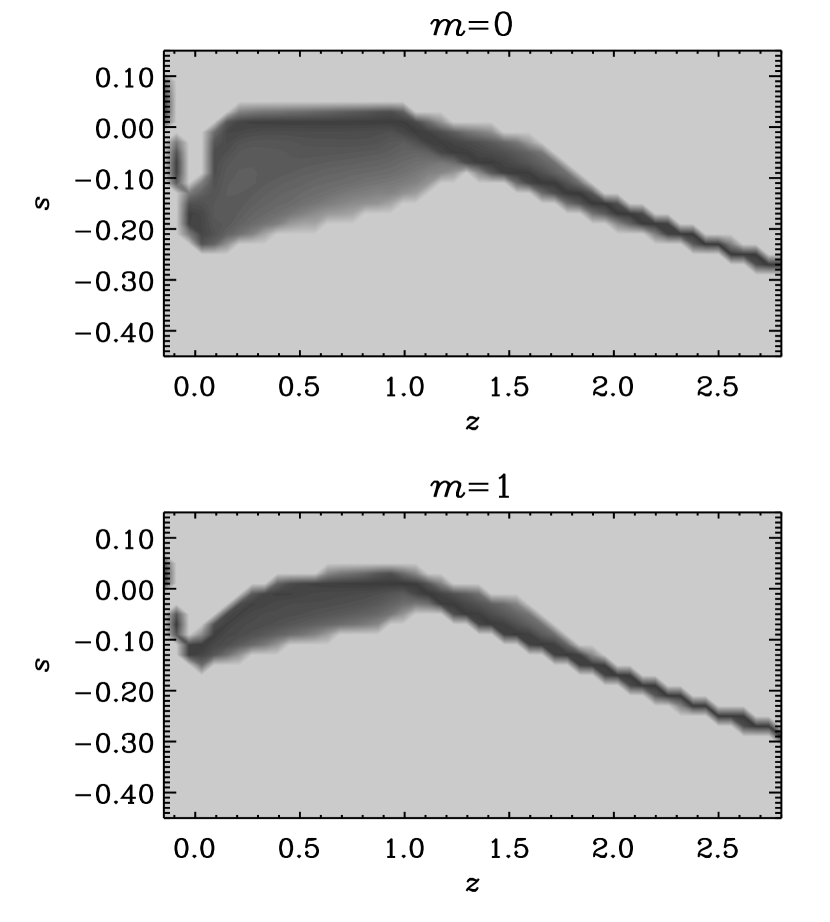
Figure 5: Entropy histograms for different values of $m$ and ${\cal F}_{\rm conv}=0.002$. Note that the range on the ordinate is reduced compared to the previous figure.

As the radiative flux is lowered, the drop of entropy and temperature at the surface becomes more sudden. This is because with less radiative diffusivity (i.e. with less radiative energy transfer) the thermal boundary layer at the top becomes thinner. At the same time the pressure must fall off smoothly, because the pressure is primarily determined by approximate hydrostatic balance. This can cause a rather pronounced density inversion near the top, as is seen in Fig. 6, which is occasionally also seen in the more realistic solar simulations.

Figure 6: Horizontally averaged density stratification for $m=-0.9$ and ${\cal F}_{\rm conv}=0.01$.

3.3 Convective and kinetic flux profiles

The mean convective flux profiles (Fig. 7) begin to converge to one and the same profile as the radiative flux is lowered. The differences between $m=-0.8$ and $-0.9$ are small, suggesting that with $m=-0.8$ or $-0.9$ the convective properties of the simulations (convective velocities and temperature fluctuations) begin to converge. However, the convective flux is not constant in the convection zone. This is because of some contribution of the kinetic energy flux, which is plotted separately in Fig. 8. As we lower the convective flux (from ${\cal F}_{\rm conv}=0.01$ to ${\cal F}_{\rm conv}=0.002$), the convective velocities decrease and therefore also the kinetic flux.

The depth of the overshoot layer is clearly reduced as we decrease the convective flux (Figs 7 and 8). This is in qualitative agreement with theories linking the depth of the overshoot layer to the magnitude of the convective velocities and hence to the convective flux (e.g. Hurlburt et al. 1994; Singh et al. 1998).

Figure 7: Comparison of the convective flux for different values of $m$ and ${\cal F}_{\rm conv}=0.01$ or 0.002 (marked by additional + symbols).

Figure 8: Comparison of the kinetic energy flux for different values of $m$ and ${\cal F}_{\rm conv}=0.01$ or 0.002 (marked by additional + symbols).

3.4 Velocity and temperature fluctuations

According to mixing length theory, the vertical velocity variance is proportional to the relative temperature fluctuation, so $\langle u_{z}^{2}\rangle\sim(\Delta T/T)\,g\ell$, where $\ell$ is the mixing length, and $g\ell\sim c_{\rm s}^{2}$. The magnitude of velocity and temperature fluctuations (denoted below by primes) is determined by the convective flux via

$$F_{\rm conv}=\langle(\rho u_{z})^{\prime}(c_{p}T)^{\prime}\rangle\sim\langle\rho\rangle\langle u_{z}^{2}\rangle^{1/2}c_{p}\Delta T.$$ (27)

This estimate implies that, apart from factors of order unity (to be determined below),

$${\Delta T\over T}\sim{\langle u_{z}^{2}\rangle\over c_{\rm s}^{2}}\sim\left({F_{\rm conv}\over\rho c_{\rm s}^{3}}\right)^{2/3}.$$ (28)

In Figs 9 and 10 we show the normalized velocity and temperature fluctuations for different runs: the profiles are basically similar. Except for the cases $m=1$ and $m=0$, the magnitude of the velocity fluctuations decreases and the magnitude of the temperature fluctuations increases as the radiative flux and/or the value of ${\cal F}_{\rm conv}$ is lowered. Also, the ratios in Eq. (28) are indeed of order unity. It turns out that this is not only valid globally, but also locally; see Fig. 11. Here we have defined the coefficients

$$k_{u}={\langle\langle u_{z}^{2}\rangle/c_{\rm s}^{2}\rangle_{\rm CZ}\over\langle F_{\rm conv}/(\rho c_{\rm s}^{3})\rangle^{2/3}},\quad k_{T}={\langle\Delta T/T\rangle\over\langle F_{\rm conv}/(\rho c_{\rm s}^{3})\rangle^{2/3}},$$ (29)

where the averages are taken over the convection zone proper, i.e. in $z_{2}<z<z_{3}$.

Figure 9: Comparison of the normalized vertical velocity fluctuations for different values of $m$ and ${\cal F}_{\rm conv}=0.01$ or 0.002 (marked by additional + symbols). The normalization factor is ${\cal F}_{\rm conv}^{-2/3}$.

Figure 10: Comparison of the normalized temperature fluctuations for different values of $m$ and ${\cal F}_{\rm conv}=0.01$ or 0.002 (marked by additional + symbols). The normalization factor is ${\cal F}_{\rm conv}^{-2/3}$.

Figure 11: Vertical profiles of the normalized mean squared vertical velocity fluctuations and temperature fluctuations, compared with the normalized convective flux raised to the power $2/3$. Note the good agreement between the three curves within the convection zone proper.

The dependence of these scaling relations (28) and (29) on Prandtl number is shown as a plot of $k_{u}$ and $k_{T}$ on Pr in Fig. 12. The dependence of $k_{T}$ on Pr is more or less unique, independent of whether the change in Pr is accomplished by changing $\nu$ or $\overline{\chi}_{2}$. By contrast, the dependence of $k_{u}$ on Pr is not unique. For constant values of $\nu$, $k_{u}$ is nearly constant, while it increases with decreasing values of $\overline{\chi}_{2}$. We explain this result as follows.

As $\overline{\chi}_{2}$ increases (Pr decreases), temperature fluctuations are smoothed out, thus decreasing $\Delta T/T$. This would decrease the convective flux (which is proportional to the product of temperature and vertical velocity fluctuations), but since the convective flux is kept constant this can only be achieved by increasing the vertical velocity fluctuations and hence $k_{u}$.

The fact that $k_{u}$ and $k_{T}$ remain Pr-dependent even at reasonably large Reynolds numbers is somewhat surprising. Our largest Reynolds number, based on the rms velocity in the convection zone proper and the depth of the unstable layer, is around 1000. It is possible that one needs to go to much larger values before $k_{u}$ and $k_{T}$ become independent of Pr.

Figure 12: Dependence of $k_{u}$ and $k_{T}$ on Pr. Note that $\nu$ is constant along solid lines and $\overline{\chi}_{2}$ and hence $m$ are constant along dotted lines. $\nu$ and $\overline{\chi}_{2}$ are given in units of $10^{-4}$, i.e. $\nu_{-4}=\nu/10^{-4}$ and $\nu_{-4}=\nu/10^{-4}$.

3.5 Morphology

Fig. 13 shows temperature (or $e$) in horizontal planes at various depths. At the top of the unstable layer the temperature displays a familiar granular pattern with cool downdraft lanes. As $m$ approaches $-0.9$ the pattern becomes generally sharper and more complex and of smaller scale. At the bottom of the convection zone ($z=1$) there are isolated cool downdrafts. For $m=-0.9$ the granular surface pattern still prevails, but this is connected with weak density stratification. As the downdrafts enter the lower overshoot layer ($z=1.5$) they become warmer. This is now due to the exterior entropy being lower than that of the downdrafts, which carry entropy from the upper convection zone.

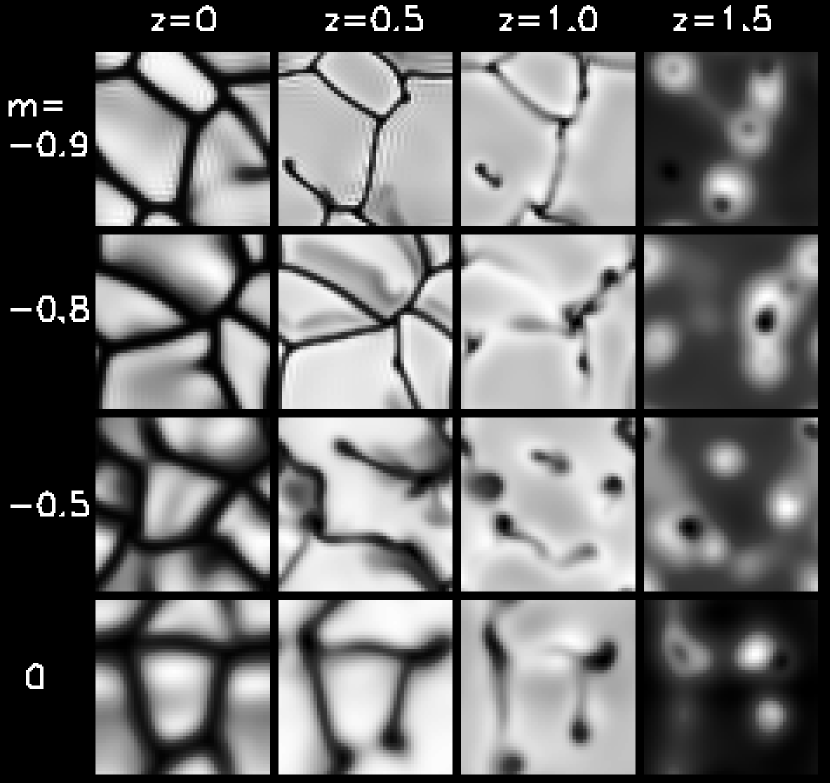
Figure 13: Horizontal slices of temperature at 4 different levels for four different values of $m$. ${\cal F}_{\rm conv}=0.01$.

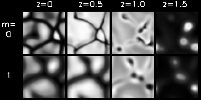
Figure 14: Horizontal slices of temperature at 4 different levels for two different values of $m$. ${\cal F}_{\rm conv}=0.002$.

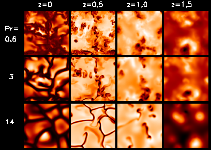
Figure 15: Horizontal slices of temperature at 4 different levels for $m=-0.9$ and three different values of $\nu$. ${\cal F}_{\rm conv}=0.01$. A resolution of $200^{3}$ meshpoints was used for Pr=0.6, and $100^{3}$ for Pr=3 and 14.

When the convective flux is decreased (${\cal F}_{\rm conv}=0.002$; see Fig. 14), the temperature pattern becomes sharper again, but the structure and the typical number of cells remains about the same. On the other hand, if $\nu$ is lowered the temperature becomes much more intermittent and of significantly smaller scale; see Fig. 15.

4 Subgrid scale models

Our next step is to compare our findings with the case where the radiative flux is replaced by a Smagorinsky subgrid scale (SGS) energy diffusion inside the convection zone (see Chan & Sofia 1986, 1989), corresponding to the limiting situation $m=-1$. For this purpose, we use the original code of Chan and Sofia. Since the formulation (solving the conservative form of the Navier-Stokes equations) and the scheme of this code (second order only) are different from that used in the previous section, we make a comparison of the results of the two codes using the previous $m=-0.9$, $\nu=0.006$ case (with a $50^{3}$ mesh). In Fig. 16, the dashed and dot-dashed curves represent results from the Nordlund & Stein (1990) code (I) and the Chan & Sofia code (II) respectively. The agreement is good.

In the SGS case, the radiative conduction and cooling outside the convective region are fixed in the same way as discussed in Sec. 2. Inside the convection zone, the numerical stability of the energy equation is maintained by a subgrid scale diffusive flux of the form $=-\chi_{\rm t}\rho T\nabla s$, where $\chi_{\rm t}$ is the SGS diffusivity. The numerical stability of the momentum equation is maintained by a SGS kinematic viscosity

$$\nu_{\rm t}=0.32\,\triangle x\triangle z\,(2\mbox{\boldmath$\mbox{\boldmath${\sf S}$}{}^{2}$})^{1/2}.$$ (30)

where $\triangle x$ and $\triangle z$ are the horizontal and vertical grid widths respectively. The ratio between $\nu_{\rm t}$ and $\chi_{\rm t}$ is fixed throughout the convection zone.

Figure 16: Comparison of SGS models (solid and dotted lines, $m=-1$) with direct calculations ($m=-0.9$). The dashed and dash-dotted lines refer to Code I used in Sec. 3 (Nordlund & Stein 1990) and Code II used in the present section (Chan & Sofia 1986). While the $m=-1$ and $m=-0.9$ models are very similar in the mean density stratification and the scaled temperature fluctuations, there are significant differences in the mean entropy profile and the scaled vertical velocity fluctuations.

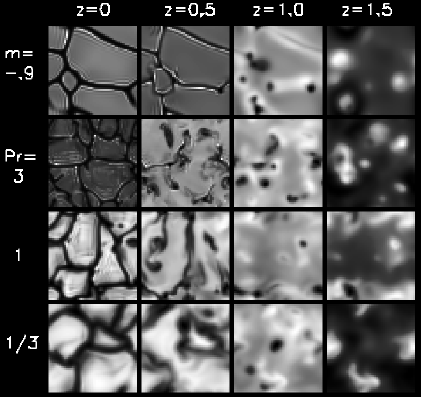
Figure 17: Horizontal slice of temperature for $m=-0.9$ and SGS model using three different values of the Prandtl number $\mbox{Pr}=\nu_{\rm t}/\chi_{\rm t}$. ${\cal F}_{\rm conv}=0.01$. All calculations here use a $50^{3}$ mesh.

In the original code of Chan & Sofia (1986) the effective Prandtl number, ${\rm Pr}_{\rm t}\equiv\nu_{\rm t}/\chi_{\rm t}$, was chosen to be 1/3. However, in order to facilitate comparison with the models discussed previously, where we varied the thermal diffusivity, we now consider three models with ${\rm Pr}_{\rm t}=1/3$, 1, and 3. All three models have the same total flux $F_{\rm tot}=0.01$ and use a $50^{3}$ mesh. In the SGS case the flow still shows the usual granular pattern at the surface; see Fig. 17. Smaller diffusivity $\chi_{\rm t}$ produces thinner intergranular lanes and decreases the size of the smallest granular structures; it is consistent with the trend shown in the previous section. Compared to the constant $\nu$ case with the same mesh size (Fig. 13), the SGS patterns show more vortical features and indicate more vigorous turbulence. In the case with the largest $Pr$, however, the temperature field is getting a little noisy; the thermal diffusivity is already too small to give reliable results. In Fig. 16 we plot the mean entropy, density, as well as velocity and temperature fluctuations for ${\rm Pr}_{\rm t}=1/3$ and $1$.

Since $\nu_{\rm t}$ depends on the local strength of the turbulence, it is not uniform anymore. Its horizontal mean varies with depth and reaches a maximum near the top of the convection zone. The range of the mean values ($0.0015-0.0030$), however, is quite limited and they are less than half of that used in the previous comparable case ($m=-0.9$, $\nu=0.006$ and same mesh size). Relative to this case, the effective Reynolds numbers of the SGS models are thus considerably larger. The SGS diffusivity $\chi_{\rm t}$, on the other hand, ($\propto{\rm Pr}_{\rm t}^{-1}$ approximately) varies by almost an order of magnitude across the different models and are larger than the $\chi$ of the low-resolution $m=-0.9$ case (ratio $\approx 1.1-10$). The temperature fluctuations of the SGS models are thus smaller (difference $\approx 20-30\%$). To deliver a comparable amount of convective energy flux, the value of the vertical rms velocity for the SGS models is considerably higher than that of the $m=-0.9$ model. This is accomplished by a somewhat steeper entropy gradient in the convection zone. The density stratification is similar. Given that the turbulence has become more vigorous, the kinetic energy flux is now increased by almost a factor of 2 to about $35\%$ of the total flux. Part of that ($\sim 9\%F_{\rm tot}$) is compensated by the subgrid scale convective flux, and the rest is balanced by the enhanced enthalpy flux.

5 Solar simulations

Figure 18: Total, enthalpy, radiative and kinetic energy fluxes for the solar simulations. Crosses are case $\mbox{Pr}_{\rm t}=0.3$ and lines are case $\mbox{Pr}_{\rm t}=3$. When the diffusive energy flux is larger, the kinetic energy flux increases and the enthalpy flux decreases slightly.

Figure 19: Average entropy vs. depth. (Here the Prandtl number is written as $\sigma$.) Larger energy diffusion produces a slightly smaller entropy gradient just below the surface.

Figure 20: Average density vs. depth. Larger energy diffusion leads to a less extended atmosphere.

Figure 21: Histogram of the entropy distribution at a depth of 1.5 Mm. For larger diffusive energy transfer, smaller Prandtl number, the lowest entropy fluid is destroyed and the exponential distribution becomes steeper.

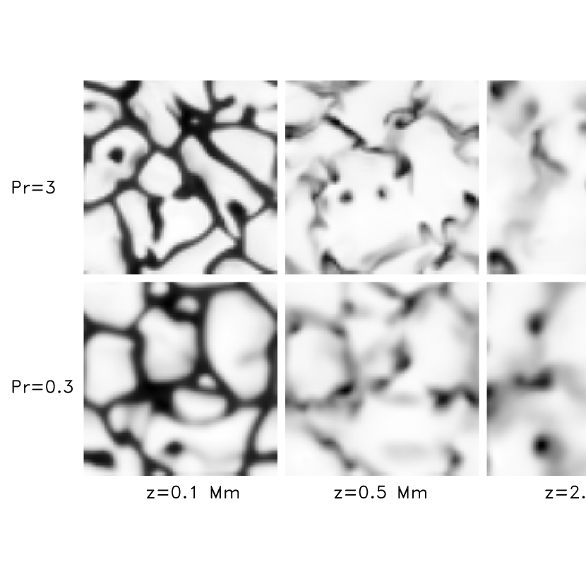
Figure 22: Horizontal slices showing the temperature at depths of 0.1, 0.5 and 2.0 Mm for two values of the Prandtl number. Dark is low temperature and light is high temperature. Each panel is scaled independently. Smaller energy diffusion, larger Prandtl number, allows smaller scale temperature structures to exist.

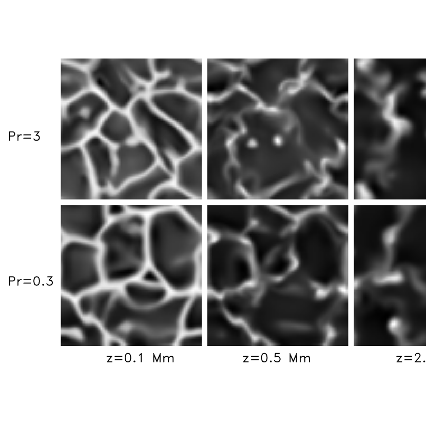
Figure 23: Horizontal slices showing the vertical velocity fluctuations at depths of 0.1, 0.5 and 2.0 Mm for two values of the Prandtl number. Dark is upward velocity and light is downward velocity. There is little difference in the scale of the velocity structures between these high and low energy diffusion cases.

We have also made two simulations of near surface solar convection with Prandtl numbers $\mbox{Pr}_{\rm t}=\nu_{\rm t}/\chi_{\rm t}=0.33$ and $3.3$, using realistic physics, with a low resolution of $63^{3}$ (for details see Nordlund & Stein 1990; Stein & Nordlund 1998). Here the radiative flux vanishes below the surface but there is numerical energy diffusion with the above ratios to the momentum diffusion. The vertical energy diffusion is proportional to the gradient of the energy minus the horizontally averaged mean energy, so it is similar to the entropy diffusion used in the SGS case. The diffusion coefficients are not constant, but have terms proportional to the sound speed, the magnitude of the velocity, and the compression. They are enhanced where there are small scale velocity fluctuations and quenched in laminar regions by the ratio of the magnitudes of the third to the first derivatives of the velocity. These simulations only extend to 2.5 Mm below the surface and the convective flux is controlled by specifying the entropy of the inflowing fluid at the bottom. The simulations were run for 2 solar hours.

Larger energy diffusion (i.e. smaller Prandtl number) produces a slightly larger kinetic energy flux and a slightly smaller enthalpy flux, resulting in a 5% reduction in the net flux (Fig. 18). The energy transport switchover between radiative and convective occurs slightly deeper in the large energy diffusion case.

There are some other small alterations in the mean structure: larger energy diffusion produces a less steep mean entropy gradient at the surface (Fig. 19) and a less extended atmosphere (Fig. 20).

The low entropy fluid (which gives rise to the buoyancy work that drives the convection) is fluid that reaches the surface and radiates away its energy and entropy. Larger energy diffusion destroys the lowest entropy fluid as it descends back into the interior, by heating it up. This leads to slightly steeper exponential decline in the entropy probability distribution function and a less extended low entropy tail to the distribution (Fig. 21).

Figure 24: Histogram of the vorticity distribution at a depth of 1.5 Mm. Varying the energy diffusion by a factor of ten has only a very slight effect on the velocity and vorticity.

Increasing the energy diffusion has a clear direct influence on the temperature structures in these simulations, just as found when varying the diffusive radiative flux – larger energy diffusion produces larger more diffuse temperature structures, smaller energy diffusion allows smaller, sharper temperature structures (Fig. 22).

The velocity and turbulence, on the other hand, are little affected by this factor of ten variation in the energy diffusion (Fig. 24). Changing the resolution and hence the viscous momentum diffusion, however, has a profound affect on the turbulence (vorticity) and the velocity (Stein & Nordlund 1998). Less viscosity leads to greater turbulence, larger vorticity, as well as a velocity distribution extending to larger magnitudes in all directions but only in a small fraction of the volume.

6 Summary

There are a number of clear changes in convective properties as the diffusive radiative flux is decreased while keeping the convective flux constant in a convection simulation. First, the entropy jump near the top becomes larger and steeper and the low entropy fluid produced by cooling at the surface penetrates farther through the convection zone leading to a finite probability to find small regions with very low entropy near the bottom of the unstable layer. Second, the temperature fluctuations increase and the velocity fluctuations decrease in such a way that their product, which is proportional to the convective flux, remains approximately constant. Also, the kinetic energy flux decreases. Third, the dynamics in the overshoot layer becomes somewhat more intermittent due to a few strong downdraft plumes. Finally, in all cases the velocity and temperature fluctuations follow mixing length scaling laws; see Fig. 11.

The radiative flux really serves two different purposes: it transports heat vertically, and it keeps the model numerically stable by diffusing energy fluctuations both horizontally and vertically. Since those two properties appear to be reasonably well decoupled from each other, one might separate them by having a small vertical radiative flux plus a subgrid scale diffusive flux that keeps the model stable. It is in practice difficult to decouple the need for energy diffusion from the vertical diffusive heat transport, which one would like to keep small if one diffuses on the temperature. However, as discussed in the introduction, such a separation is possible if the diffusive flux is based on entropy or temperature fluctuations. Convective simulations with small radiative fluxes, as is appropriate for cool stars, would then be feasible. This was recently demonstrated by Miesch et al. (2000) and Brun et al. (2004) using simulations of fully spherical shells.