Estimation of Carbon Abundances in Metal-Poor Stars. I. Application to the “Strong G-band” stars of Beers, Preston, & Shectman

Abstract

We develop and test a method for the estimation of metallicities ([Fe/H]) and carbon abundance ratios ([C/Fe]) for carbon-enhanced metal-poor (CEMP) stars, based on application of artificial neural networks, regressions, and synthesis models to medium-resolution ($1-2$ Å ) spectra and $J-K$ colors. We calibrate this method by comparison with metallicities and carbon abundance determinations for 118 stars with available high-resolution analyses reported in the recent literature. The neural network and regression approaches make use of a previously defined set of line-strength indices quantifying the strength of the CaII K line and the CH G-band, in conjuction with $J-K$ colors from the 2MASS Point Source Catalog. The use of near-IR colors, as opposed to broadband $B-V$ colors, is required because of the potentially large affect of strong molecular carbon bands on bluer color indices.

We also explore the practicality of obtaining estimates of carbon abundances for metal-poor stars from the spectral information alone, i.e., without the additional information provided by photometry, as many future samples of CEMP stars may lack such data. We find that, although photometric information is required for the estimation of [Fe/H], it provides little improvement in our derived estimates of [C/Fe], hence estimates of carbon-to-iron ratios based solely on line indices appear sufficiently accurate for most purposes. Although we find that the spectral synthesis approach yields the most accurate estimates of [C/Fe], in particular for the stars with the strongest molecular bands, it is only marginally better than is obtained from the line index approaches.

Using these methods we are able to reproduce the previously-measured [Fe/H] and [C/Fe] determinations with an accuracy of $\approx 0.25$ dex for stars in the metallicity interval $-5.5\leq{\rm[Fe/H]}\leq-1.0$, and with $0.2\leq(J-K)_{0}\leq 0.8$. At higher metallicity the CaII K line begins to saturate, especially for the cool stars in our program, hence this approach is not useful in some cases. As a first application, we estimate the abundances of [Fe/H] and [C/Fe] for the 56 stars identified as possibly carbon-rich, relative to stars of similar metal abundance, in the sample of “strong G-band” stars discussed by Beers, Preston, & Shectman.

1 Introduction

Several recent papers (e.g., Norris, Ryan, & Beers 1997a; Rossi, Beers, & Sneden 1999) have pointed out that the frequency of carbon-enhanced stars in the Galaxy appears to increase at the lowest metal abundances. Continuation and expansion of ongoing medium-resolution spectroscopic follow-up of candidate low-metallicity stars (the HK survey of Beers and colleagues; Beers, Preston, & Shectman 1992, hereafter BPSII; Beers 1999; the Hamburg/ESO Survey, HES, of Christlieb and collaborators; Christlieb 2003) has indicated that the actual fraction of stars with metallicities [Fe/H] $\leq-2.0$ and carbon enhancements in excess of [C/Fe] $\simeq+1.0$ may be even higher than previously suspected, perhaps as great as 20-25%. At the lowest metallicities, e.g., for [Fe/H] $<-3.5$, the fraction of stars that are carbon enhanced at a level of [C/Fe] $\geq+1.0$ rises to 40% (Beers & Christlieb 2005). The only two stars known with [Fe/H] $<-5.0$ both exhibit extremely high [C/Fe] ratios (Christlieb et al. 2002; Frebel et al. 2005).

Recently, Cohen et al. (2005) have argued that the fraction of carbon-enhanced, metal-poor (hereafter, CEMP) stars has been overestimated by previous studies. They use a sample of some 50 high-resolution spectra of metal-poor stars selected from the HES to conclude that the fraction of CEMP stars is 14.4% $\pm$ 4%. This fraction does not differ at the two-sigma level from previous claims. Furthermore, the authors of the present paper feel that there are multiple reasons why this determination might be more properly be considered a lower limit on the actual frequency, including the procedures used to select metal-poor candidates from the HES. The question is of great significance, and needs to be revisited using larger samples of metal-poor stars with high-resolution abundance analyses, as well as with stars selected in alternative ways.

Clearly, it is important to understand the astrophysical phenomena responsible for the high frequency of CEMP stars, and to assess their impact on the early chemical evolution of the Galaxy. Lucatello et al. (2005b), for instance, have argued that the large fraction of CEMP stars at low metallicities provides evidence for an alteration in the Initial Mass Function (IMF) during these epochs to include a greater number of intermediate mass stars than are formed from the present-day IMF. The connection, if any, to the significant amounts of ionized carbon in the intergalactic medium detected in observations toward distant quasars (e.g., Ellison et al 2000; Pettini et al. 2003), may also hold important clues to the production of carbon at the earliest times. For additional details, see the discussion in Beers & Christlieb (2005).

High-resolution abundance analyses for a number of CEMP stars (Barbuy et al. 1997; Norris, Ryan, & Beers 1997b; Bonifacio et al. 1998; Aoki et al. 2000, 2001, 2002a,b,c; Norris et al. 2002; Depagne et al. 2002; Sivarani et al. 2004; Barbuy et al. 2005) indicates that a variety of carbon-production mechanisms may need to be invoked to account for the observed range of elemental abundance patterns in these stars (e.g., mass-transfer from former AGB companions, self-pollution via mixing of CNO-processed material in individual stars, the possible existence of zero-abundance “hypernovae” which may produce large amounts of carbon, etc.). Many of the CEMP stars have been shown to be members of binary systems (Preston & Sneden 2001; Tsangarides, Ryan, & Beers 2004; Lucatello et al. 2005a). The majority, but interestingly not all, of the CEMP stars are associated with neutron-capture-element enhancement (in particular from the s-process; see Aoki et al. 2003). At least one member of the growing class of highly r-process-enhanced, metal-poor stars, CS 22892-052 (see Sneden et al. 1996, 2003) also exhibits large C (and N) overabundances relative to the solar ratios, although the origin of the carbon enhancement and the r-process enhancement may well be decoupled from one another. It is surely not a coincidence that the two most iron-deficient stars yet identified, HE 0107-5240 (Christlieb et al. 2002; Christlieb et al. 2004), and HE 1327-2326 (Frebel et al. 2005) with [Fe/H] = –5.3 and –5.6, respectively, also exhibit carbon overabundances that are the highest yet reported amongst extremely metal-poor stars, on the order of [C/Fe] $\simeq+4.0$. Much clearly remains to be learned about the nature, origin, and evolution of the many classes of CEMP stars in the Galaxy.

Recent analysis of stellar spectra from the Sloan Digital Sky Survey (Margon et al. 2002; Downes et al. 2004) has led to the claim that at least 50% of the carbon-enhanced stars in the Galaxy are probably dwarfs. The working hypothesis is that the majority of these stars are the result of mass-transfer episodes from a now-extinct more massive companion. Totten & Irwin (1998) have called attention to the presence of (apparently) intermediate-mass stars, still in their AGB phase, that may have been stripped from the Sagittarius dwarf galaxy, and which provide a potentially strong probe on the clumpiness and axial symmetry of the Galaxy (Ibata et al. 2001).

In order to quantify and understand the varieties and mechanisms for explaining the origin of CEMP stars it is necessary to develop procedures by which [Fe/H] and [C/Fe] measurements may be rapidly obtained for as large a number of stars as possible. Ideally, this should be based on medium-resolution (1-2 Å) spectroscopy, since this information is already available for many thousands of metal-poor stars from the HK and HES follow-up campaigns, and will be available for hundreds of thousands of stars as new-generation surveys expand (e.g., SDSS: York et al. 2000, RAVE: Steinmetz 2003, and SEGUE: The Sloan Extension for Galactic Understanding and Exploration, which is part of the extension to the SDSS, known as SDSS-II).

In this paper we obtain a calibration of methods for rapid analysis of CEMP stars, and apply it to the sample of “strong G-band” stars from the HK survey noted by BPSII. In §2 we describe the selection of the calibration stars and the acquisition and analysis of the spectroscopic and photometric data used in this study. In §3 we describe the training and application of an Artificial Neural Network (ANN) approach, a regression approach, and a spectroscopic fitting approach. Application of our calibration to the “strong G-band” stars of BPSII is reported in §4. In §5 we discuss the distribution of carbon abundances derived for these stars. A summary of our results and comments on future applications of these techniques is presented in §6.

2 Selection of Calibration Stars and Observational Data

In the assembly of our calibration sample we have endeavored to include metal-deficient stars with as wide a range of physical parameters (T$\rm{eff}$, log g, [Fe/H]) and known carbon abundances as possible. Fortunately, recent interest in the nature of CEMP stars has greatly increased the number of suitable calibration stars. We have combined these objects with modern analyses of additional metal-poor stars in order to better cover the range of carbon abundances known to exist amongst stars in the halo of the Galaxy (e.g., $-1.0\leq{\rm[C/Fe]}\leq+4.0$). Although we would have liked to include significant numbers of dwarfs in this exercise, there are only a handful of such stars with well-measured carbon abundances that exceed the solar ratio of [C/Fe], so out of necessity our calibration sample is dominated by subgiants and giants.

We also require medium-resolution spectra for each star in the calibration sample. An initial effort (reported by Rossi et al. 1999) revealed that there were ranges of the calibration space that needed to be filled in with new medium-resolution spectroscopy of stars having available high-resolution carbon abundance determinations. Over the past few years we have acquired these data during the course of ongoing HK and HES spectroscopic follow-up campaigns.

2.1 Photometry

The broadband $V$ magnitudes and $B-V$ colors for our calibration stars are taken either from the SIMBAD database, or (for the majority of the HK survey calibration stars) from BPSII, McWilliam et al. (1995), or Beers et al. (2005, in preparation). It was recognized early on that $B-V$ colors are less than ideal for use in the estimation of carbon abundances in metal-poor stars, owing to the (in some cases) rather significant alteration of the observed flux in these bands due to the presence of molecular CH, CN, and C₂ features. This is particularly true for the most carbon-rich and/or cooler stars. One might attempt to use the $HP2$ index, a band-switched measure of the strength of the absorption line H-$\delta$ (as defined by Beers et al. 1999), as an alternative temperature indicator. Although this is useful for warmer stars, e.g., those with T${}_{\rm eff}>5000$ K, for cooler stars $HP2$ weakens precipitously, is subject to greater measurement errors, and loses some of its sensitivity to stellar temperature. Hence, we are fortunate that we can now take advantage of the reasonably high-quality near-infrared $JHK$ photometry that has recently become available from the 2MASS project (Cutri et al. 2003). The application of $J-K$ colors from 2MASS provides a indicator of stellar temperature that is less sensitive to molecular carbon bands, and furthermore, is much less dependent on foreground reddening than is the $B-V$ color.

Table 1 presents the available photometry for our calibration stars. Column (1) lists the star name. Columns (2) and (3) provide the $V$ magnitude and $B-V$ color, respectively. In column (4) and (5) we list the $J$ magnitude and $J-K$ color, and their associated errors, as reported in the 2MASS Point Source Catalog. The reported photometry is the “default magnitude” information provided in this catalog. Errors in the $J-K$ colors are obtained using the square root of the quadratic sum of the individual errors reported for the $J$ and $K$ magnitudes. We checked all of the pertinent photometric quality and contamination flags listed in the 2MASS Point Source Catalog for potentially problematic stars, and eliminated those stars from further consideration.

Reddening estimates for these stars was obtained from application of the maps of Schlegel, Finkbeiner, & Davis (1998), which have superior spatial resolution and are thought to have a better-determined zero point than the Burstein & Heiles (1982) maps. In cases where the Schlegel et al. estimate exceeds $E(B-V)_{S}$ = 0.10, we follow the procedures outlined by Bonifacio, Monai, & Beers (2000) to reduce these estimates by 35%, and obtain an adopted estimate of reddening, $E\;(B-V)_{A}$.

In the case of a few of the brighter (nearby) calibration stars, the suggested reddening was still apparently too high, hence we have assumed zero reddening in these instances. The final adopted reddening is listed in column (6) of Table 1. Columns (7) and (8) list the de-reddened $(B-V)_{0}$ and $(J-K)_{0}$ colors, respectively, where we have adopted $E(J-K)=0.56\;E(B-V)_{A}$.

2.2 Spectroscopic Observations

Medium-resolution spectroscopic data for many of the calibration stars in the present paper were obtained with the KPNO 2.1m, the Isaac Newton 2.5m on La Palma, the Las Campanas 2.5m, and the Palomar 5m telescopes. The ESO 1.5m telescope was also used to obtain observations for a number of the calibration stars discussed herein, as was the Siding Spring Observatory 2.3m telescope. A small number of additional observations were obtained with the Kitt Peak National Observatory 4m telescope, the CTIO 4m telescope, the Anglo-Australian 3.9m telescope, and the McDonald Observatory 2.7m telescope.

A complete discussion of the observing techniques and data reduction procedures that were followed is presented in Beers et al. (1999), to which we refer the interested reader. The spectra employed cover (at least) the wavelength region $\lambda\lambda 3700-4500$ Å, at resolutions between 1 and 2 Å (2.5 pixels). Signal-to-noise ratios (at 4000 Å) for the spectra varied from a minimum of 10/1 to greater than 30/1, with a typical value on the order of 20/1 per pixel. Sample spectra for several of the calibration stars, covering a range of T_eff and [C/Fe], are shown in Figure 1. Since the calibration spectra were taken as part of observing runs dedicated to survey efforts, no flux calibrations are available.

Figure 1: Example medium-resolution spectra for calibration stars covering a range of T_eff and [C/Fe]. The warmer stars are at the top; the cooler stars are at the bottom. The left-hand panels show stars with low values of [C/Fe], while those on the right-hand panels show stars with moderate to high abundances of [C/Fe]

For the present calibration we require measurements of the line indices $KP$, a (band-switched) pseudo-equivalent width measure of the CaII K line, and $GP$, a fixed 15-Å wide band measure of the strength of the CH G-band. The linebands and sidebands for these two estimators are listed in Table 2. Repeat observations of these stars indicates that the determination of an individual line index is generally accurate to on the order of $\sim 10$%.

Figure 2 indicates, for two CEMP stars of moderate and high [C/Fe] values, the location of the linebands and sidebands for the $KP$ and $GP$ indices. The method of estimating the pseudo-equivalent widths on which these indices are based employs a linear estimation of the local continuum between the sidebands. As can be appreciated from inspection of this Figure, we do not expect any difficulties with the estimate of $KP$, except perhaps in cases where extremely carbon-rich stars might compromise the sidebands of this index. By calibrating estimates of [Fe/H] directly from stars that exhibit a wide range of carbon enhancements, as discussed below, we expect to be fairly insensitive to changes in $KP$ that might be introduced, e.g., by strong molecular carbon features which can occur in the region of CaII K. By way of contrast, comparison of panels (b) and (d) of Figure 2, for CS 22892-052 and CS 29498-043, respectively, indicates that there are certainly concerns raised in the choice of the continuum for the more carbon-enhanced star, CS 29498-043. In the case of this star, both the blue and the red sideband are buried in absorption from molecular carbon features, which may lead to difficulties with the determination of the $GP$ index. Inclusion of such extreme stars in our calibration set may partially relieve this problem, but caution should be employed for application of our line-index techniques for similar extreme stars.

Figure 2: Location of the line indices $KP$ and $GP$ for two CEMP stars of moderate (CS 22892-052) and high (CS 29498-043) carbon enhancement, respectively. The open rectangles indicate the range over which the sidebands are estimated. The hatched rectangles indicate the range over which the linebands are estimated. Note that while one might expect reasonable [C/Fe] results for stars like CS 22892-052, caution must be employed for stars like CS 29498-043, where the sidebands are buried in molecular carbon features.

The spectroscopic observations of the calibration stars are summarized in Table 3. Column (1) lists the star name. In column (2) we list the telescopes involved with the acquisition of the medium-resolution spectra, using codes defined in the table end notes. The $KP$ and $GP$ line indices are listed in columns (3) and (4), respectively. The remaining columns in this table are described below.

3 Calibration of [Fe/H] and [C/Fe]

We have investigated three alternative techniques for obtaining carbon abundance estimates of metal-deficient stars, an ANN approach, a regression approach, and spectral synthesis. We describe the calibrations of these approaches separately below.

For all of these exercises we require independent knowledge of [Fe/H] and [C/Fe], which we obtain primarily from the recent literature. In a few cases, in particular for the more metal-rich stars, we have had to “reach back” to include a few classic results based on older data. Table 3 lists the pertinent information for each star. In columns (5)-(7) we list the adopted [Fe/H], [C/H], and [C/Fe], respectively. The sources used in order to obtain these numbers (generally from an average of the reported values) are listed in column (8). For a few stars new analyses appeared quite recently; in some (but not all) cases, we altered our adopted values to take this new information into account. For the spectral synthesis method described below, it is also necessary to adopt values of the physical parameters of the pertinent stellar models used. We obtain these based on average values of the parameters T_eff, log g, [Fe/H], and $\xi$ from the listed sources, and present these values in Column (9). Note that, for consistency of the spectral synthesis modeling with the predicted [C/Fe] for the BPSII “strong G-Band” stars discussed below, we employed an input microturbulance value of $\xi=2.0$ km/sec for estimation of the [C/Fe]_S values, as discussed below.

3.1 Training of an Artificial Neural Network and a Regression Alternative

Artificial Neural Networks are playing a growing role in the analysis of astronomical data, as they have a number of advantages over more traditional approaches to data analysis (for a more complete discussion of applications of ANNs to spectroscopic analyses, see Snider et al. 2001). Here we present a particularly straightforward application. We seek to estimate [Fe/H] from the $KP$ indices and $(J-K)_{0}$, and [C/Fe] based on two alternative sets of inputs: (1) $KP$, $GP$, and $(J-K)_{0}$, and (2) from the $KP$ and $GP$ indices alone. In both cases, we actually make use of the log₁₀ of the $KP$ and $GP$ indices, so that they are on the same logarithmically varying scale as the photometric inputs and the output quantities.

We have also explored the use of a multiple regression approach, similar to that used by Beers et al. (1999) for the prediction of [Fe/H] based on the $KP$ index and $(B-V)_{0}$ color, in order to obtain [Fe/H] and [C/Fe] (although here we employ $(J-K)_{0}$ colors). We prefer the ANN approach for two reasons. First, one can train a suitable network very quickly, which allows considerable flexibility in testing for the presence of potential outliers that could influence the final results. Secondly, the ANN approach allows for non-linear interactions of the predictor variables over the parameter space, as well as for different interactions of the predictor variables over the calibration space, whereas a traditional regression approach forces a particular regression model to apply over the entirety of the calibration space. As a final justification, as new (or improved) calibration data become available, the ANN approach allows for rapid retraining. Many users may be more familiar with the usual regression techniques, hence we have made available approximate regression relationships for our predictions that reasonably reproduce the results of the ANN approaches.

A first-pass training of the two sets of ANNs was accomplished using the inputs given above, and six hidden nodes, in order to predict the desired outputs [Fe/H] and [C/Fe]. Although it is possible to simultaneously predict the two output variables, our experiments suggested that (slightly) better results were obtained using dedicated networks for each output. The networks trained to predict single variables exhibited scatter in the derived abundances that were typically 10-20% lower than the networks that predicted the two variables at once. In order to differentiate the various networks we define them as follows:

$${\rm[Fe/H]}_{\rm A}=f\;[LKP,(J-K)_{0}]$$

$${\rm[C/Fe]}_{\rm A}=f\;[LKP,LGP)]$$

In the above expressions $LKP$ and $LGP$ indicate the log₁₀ of the $KP$ and $GP$ indices, respectively. We also trained a network for estimation of [C/Fe] that took advantage of using available $(J-K)_{0}$ photometry as an additional input, but this produced very little improvement in the residuals for [C/Fe], hence we decided to proceed with the generally more applicable estimate that does not require photometry as an input.

For calibration of these networks, 60% of the data is used as a training subsample, while 20% of the data is set aside for a testing subsample. The remaining 20% of the data, which is never seen by the ANNs, is used as a validation set in order to obtain an independent indication of the accuracy with which the desired outputs can be predicted. We also tested the stability of the networks by drawing ten different sets of training, testing, and validation subsets, and looking for any indication of inconsistency in the predictions of the output quantities. None were found.

During the course of our training of the ANNs, it was immediately noticed that the ANNs had difficulty in obtaining reasonable estimates of [Fe/H] for stars with [Fe/H] $>-1.0$, a problem that is almost certainly due to saturation, or near saturation, of the $KP$ index for metal-rich and/or very cool stars. Similar problems were encountered in the Beers et al. (1999) calibration, but were addressed by introduction of a second estimator, the Auto-Correlation Function (ACF). A similar adjustment is made difficult for carbon-rich stars, because the molecular carbon bands themselves can have a large effect on an ACF, at least as defined in the Beers et al. (1999) paper.

Even after removal of stars that were expected to present problems because of possible saturation effects, it was clear that a number of stars in the calibration set exhibited rather large deviations, so the training was repeated with these stars set aside. Such “problem” stars might be also indicative of poorly measured $KP$, $GP$, or $(J-K)_{0}$, or errors in the high-resolution estimates of [C/Fe] and/or [Fe/H] reported for the calibration stars themselves. Our final results are summarized in Table 4. Column (1) of Table 4 reports the star names, column (2) lists the adopted external estimate of [Fe/H] from the literature, column (3) lists the estimate of [Fe/H] obtained from the ANN analysis, [Fe/H]_A, along with its associated residual relative to the literature value of [Fe/H], and column (4) lists the estimate of [Fe/H], [Fe/H]_R, obtained from the regression analysis, described below, along with its associated residual. Column (5) lists the adopted literature value of [C/Fe], column (6) lists the estimate of [C/Fe] obtained from the ANN analysis, [C/Fe]_A, along with its associated residual relative to the literature value of [C/Fe], and column (7) lists the estimate of [C/Fe] obtained from the regression analysis, [C/Fe]_R, described below, along with its associated residual. Column (8) indicates the grouping of the calibration stars into several bins in T_eff, [Fe/H], and [C/Fe], respectively, as listed in the table end notes. We use these bins below to explore the typical residuals from the two methods used to estimate [Fe/H], and the three methods used to estimate [C/Fe] over the calibration space. Column (9) lists the spectral synthesis estimate of [C/Fe], [C/Fe]_S, as described below, and its residual with respect to the literature value of [C/Fe]. Column (10) indicates, with an “X”, the stars which were dropped from the [C/Fe] calibration due to their large residuals in estimation of [C/Fe] by the ANN approach (dropped stars are those with an absolute [C/Fe]_A residual larger than 0.6 dex).

Figures 3(a) and 3(b) show the distribution of [C/Fe] and [C/H], respectively, as a function of [Fe/H], for the stars that were used for our final calibration exercise. Figures 3(c) and 3(d) show the distribution of these same quantities as a function of T_eff. As can be appreciated from inspection of these figures, it would be desirable to obtain additional observations of well-studied stars with [C/Fe] $>+1.0$ for metallicities [Fe/H] $>-2.0$. Similarly, we would benefit from observations of additional stars with Teff $>5500$ K.

Figure 3: Distribution of adopted [C/Fe] and [C/H] from the recent literature for the accepted calibration stars as functions of [Fe/H] (panels a and b), and as a function of Teff (panels c and d).

Figure 4 shows the distribution of positive and negative residuals, with the size of the points scaled to be proportional to the size of the individual residual, for the ANN determinations of [Fe/H] and [C/Fe] with respect to the adopted literature values, as functions of the predictor variables used in the estimates. Inspection of the patterns and sizes of the residuals indicates that, at least over the calibration space we have considered, the residuals are evenly distributed in their sizes and signs. More quantitative estimates of the residuals are presented in Table 5, discussed below.

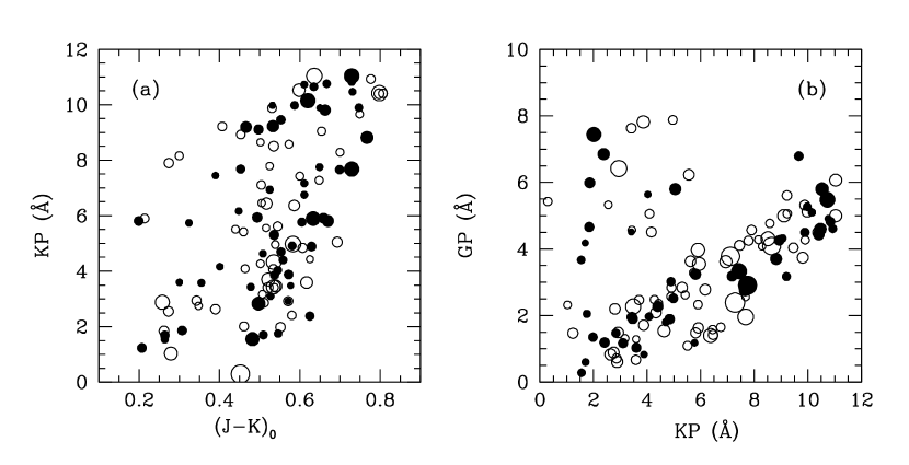
Figure 4: (a) Distributions of positive and negative residuals of the ANN estimates of [Fe/H], with respect to adopted literature values, for the accepted calibration stars over the calibration space defined by $KP$ and $(J-K)_{0}$. (b) Distribution of positive and negative residuals of the ANN estimates of [C/Fe], with respect to the adopted literature values over the calibration space defined by $GP$ and $KP$. In both cases, positive residuals are indicated by filled circles, while negative residuals are indicated by open circles. The size of each point is scaled to be proportional to the size of the residual.

Approximate regression relations for [Fe/H] and [C/Fe] are:

$${\rm[Fe/H]}_{\rm R}=-1.272\;(0.196)-1.562\;(0.588)\;LKP$$

$$+3.906\;(0.411)\;LKP^{2}-4.045\;(0.203)\;(J-K)_{0}$$

$$\epsilon=0.25\;,\;{\rm R}^{2}=0.95$$

$${\rm[C/Fe]}_{\rm R}=1.698\;(0.071)-3.403\;(0.108)\;LKP$$

$$+1.995\;(0.090)\;LGP$$

$$\epsilon=0.26\;,\;{\rm R}^{2}=0.95$$

In the above, $\epsilon$ indicates the expected prediction error of the estimate, while R² is the total variance that can be accounted for by the regression relationship. The quantities in parentheses following each of the coefficients are their one-sigma errors. As in the case of the ANNs, a regression was performed that predicts [C/Fe] based on the inclusion of $(J-K)_{0}$, in addition to $LKP$ and $LGP$, but little improvement over the regression that did not involve photometry was obtained.

3.2 The Spectral Synthesis Approach

The first stage in the synthesis calculations requires that reasonable first guesses be made for the pertinent physical parameters of the stellar atmospheres that are employed. In the case of the calibration stars, these were already known based on previous high-resolution studies. For the program stars, the “strong G-band” stars of BPSII, we employed estimates of [Fe/H] derived from the ANNs, and approximations of T_eff and log g, as described below.

We computed synthetic spectra of calibration and program stars over essentially the entire wavelength range of the CH G-band, 4190 Å $\leq$ $\lambda$ $\leq$ 4425 Å. The current version of the LTE line analysis code MOOG (Sneden 1973) was used to generate these spectra. Stellar atmospheres were interpolated from the grid of ATLAS9 models by Castelli & Kurucz (2003), using software developed by A. McWilliam and I. I. Ivans (private communication). The values of T_eff, log g, and [M/H] that were adopted for each star are provided in column (9) of Table 3 (calibration stars) and Table 7 (program stars). We culled Kurucz’s atomic and molecular line database to produce the input line list of more than 3000 neutral, singly ionized, and CH molecular species. We also assumed ${\rm{}^{12}C/^{13}C}$ = 10, but this parameter also did not strongly influence the derived C abundances. We did not include the CN lines that exist in the 4190–4215 Å region, after preliminary synthetic spectrum experiments showed that CN absorption produced almost no effect on the derived C abundances, which mostly were estimated from the 4230–4370 Å region.

In our computations we assumed solar abundances in good agreement with those recommended by Lodders (2003). We also adopted log $\epsilon$(C)_⊙ = 8.56 and log $\epsilon$(O)_⊙ = 8.92, which were generally employed prior to their re-examination by Allende Prieto et al. (2001,2002) and Holweger (2001). The best values of these two abundances now appear to be approximately log $\epsilon$(C) = 8.4 and log $\epsilon$(O) = 8.7, about 0.2 dex lower. Adoption of these new photospheric values would lead only to a uniform offset from our quoted C abundances.

Some caution should be observed, however, in interpreting our abundances for the coolest, most metal-rich stars, for which CO formation potentially could have a larger influence on the derived C abundance. Relative [X/Fe] abundances of the $\alpha$-elements O, Mg, Si, and Ca were set to typical values for halo stars, [$\alpha$-element/Fe] = +0.4. Finally, we assumed a uniform value for microturbulent velocity, v_t = 2 km s^-1 (tests conducted with $\pm$0.5 variations in this parameter demonstrated the relative insensitivity of derived C abundance to v_t). Our tests indicated that small changes in carbon isotopic ratios, $\alpha$-element enhancements, and microturbulance produced only small variations ($\lesssim$0.1 dex) in our estimated carbon abundances.

The synthetic spectra were computed for different values of [C/Fe], and smoothed with a Gaussian function to match the resolution of the observed spectra. Setting the continuum levels in the observed spectra could not be reliably done from inspection of the spectra themselves. The data were obtained with many different several telescope/instrument configurations, all without the benefit of flux calibration, hence the continuum shape is determined by the convolution of the actual stellar continuum with the instrumental response function. The spectra are relatively low resolution for abundance work; in cases of strong CH, CN, and/or C₂ bands true continuum regions are difficult to identify. However, for each instrumental setup, at least a few warm, very metal-poor, very weak-CH stars were observed. We used specialized software (Fitzpatrick & Sneden 1987) to co-add these weak-lined spectra and then interactively fit spline functions through their easily identified continuum points spaced at roughly 50 Å intervals. The resulting approximate continuum curves were divided into the spectra of all of the calibration and program stars.

After the spectra were flattened, the computed and observed spectra were visually compared; difference plots between the two were also compared. These led to carbon abundances estimated to the nearest 0.05 dex, for stars with high signal-to-noise spectra and moderate-to-strong CH band strengths. For stars with barely detectable CH features and/or noisy spectra, the errors on the abundance estimates are larger. The results of the synthesis calculations of [C/Fe] for the calibration stars are provided in column (9) of Table 4, along with the residual obtained from a comparison with the results from the high-resolution studies. For moderate to higher signal-to-noise spectra, the typical error in estimation of [C/Fe] by the spectrum synthesis technique, as judged from the residuals with respect to the external adopted values of [C/Fe], is on the order of 0.20-0.25 dex. In column (9) of Table 4 we note with single colons those abundances that are likely to have larger uncertainties, as judged by the quality of the fit to the observed spectra. Double colons indicate stars with very poor fits, which should be considered quite uncertain.

Figure 5 shows several examples of the synthetic/observed spectrum matches for the calibration stars. In this Figure, we show two examples for each of our four bins in T_eff, one each with low [C/Fe] ([C/Fe]${}_{\rm S}\leq 0.0$), and one each with large [C/Fe] ([C/Fe]${}_{\rm S}>+1.0$). These are the same stars for which the entire available spectra are shown in Figure 1.

Figure 5: Examples of the spectral synthesis fits for calibration stars covering a range of T_eff and [C/Fe]. The warmer stars are at the top; the cooler stars are at the bottom. The left-hand panels show stars with low values of [C/Fe], while those on the right-hand panels show stars with moderate to high abundances of [C/Fe]. The values of the adopted atmospheric model parameters are indicated (T_eff/log g/ [M/H]). The data are shown as filled circles. The lines indicate the fits obtained from various input values of [C/Fe] differing by 0.5 dex; the adopted best-fit is shown as a bold line.

As noted above, our calibration sample is unavoidably weighted toward the inclusion of subgiants and giants, so the effect of surface gravity on our estimation of [C/Fe] could not be adequately determined from this sample alone. Instead, we explored this issue by synthesizing spectra of higher gravity stars, up to log g $=+5.0$, and applying our present techniques to their analysis. These experiments indicated that, over our calibration space, the effect of higher surface gravity introduced shifts of from a few tenths of a dex to (in the most extreme cases) 0.5 dex in the determination of [C/Fe].

3.3 Comparison of the Various Methods

In this section we consider the accuracies of the methods we employ in more detail. First, we examine plots of the residuals of the predicted [Fe/H] and [C/Fe] for the three methods as functions of their individual predictor variables and as compared to our adopted literature values of these quantities. We then quantitatively consider the accuracies of the methods we have explored for estimation of [Fe/H] and [C/Fe], first globally, and then across the various bins in T_eff, [Fe/H], and [C/Fe] as defined in the end notes of Table 4.

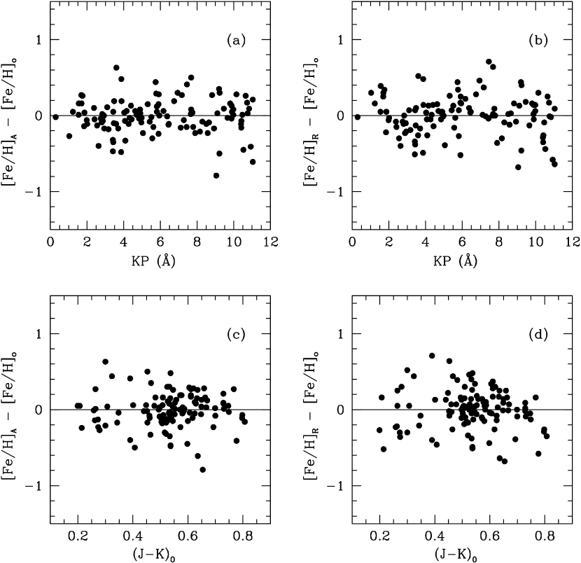
Figure 6: (a) Distributions of residuals of the estimated [Fe/H] based on the ANN approach, [Fe/H]_A, as compared to the adopted literature value, [Fe/H]${\rm o}$, as a function of the predictor variable $KP$. (b) The same as in panel (a), but for [Fe/H]_R. (c) Distributions of residuals of the [Fe/H]_A as compared to [Fe/H]${\rm o}$, as a function of the predictor variable $(J-K)_{0}$. (d) The same as in panel (c), but for [Fe/H]_R.

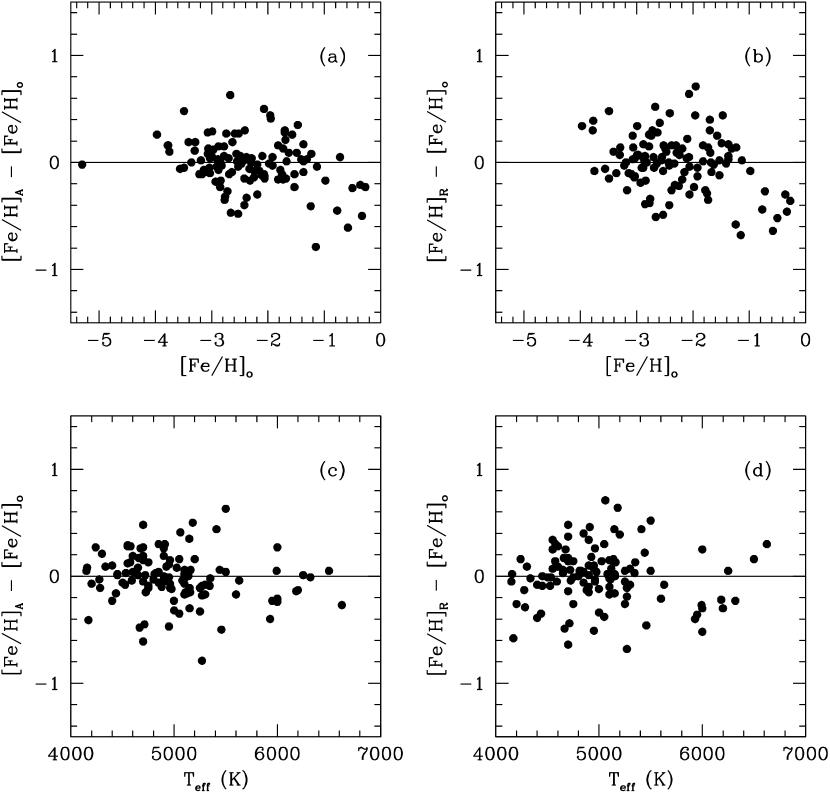
Figure 7: (a) Distributions of residuals of the estimated [Fe/H] based on the ANN approach, [Fe/H]_A, as compared to the adopted literature value, [Fe/H]_o, as a function of [Fe/H]_o. (b) The same as in panel (a), but for [Fe/H]_R. Note that the residual for HE 0107-5240 is not shown (see text). (c) Distributions of residuals of the [Fe/H]_A as compared to [Fe/H]${\rm o}$, as a function of T_eff. (d) The same as in panel (c), but for [Fe/H]_R.

Figure 6 shows the residuals in the determination of the estimated [Fe/H], as compared to the individual predictor variables $KP$ and $(J-K)_{0}$, for both the ANN and regression approaches. As can be seen from inspection of this Figure, the residuals are distributed similarly over the predictor variables for both techniques. Some of the largest negative residuals in the estimates of [Fe/H] occur when either $KP$ is large, or for the redder stars; at these extremes the $KP$ index is approaching saturation. Figure 7 shows the same sets of residuals as a function of the adopted literature values of [Fe/H] and T_eff. Note that the residual for HE 0107-5240 is not plotted in panels (b) and (d), since it is extremely large; the polynomial used for the estimate of [Fe/H]_R for this [Fe/H] $=-5.3$ star provides an unrealistic estimate of its metallicity. The larger negative residuals for [Fe/H] $>-1$ are clearly evident in panels (a) and (b).

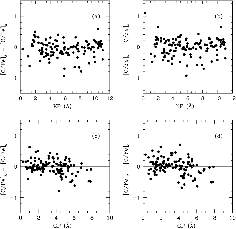
Figure 8: (a) Distributions of residuals of the estimated [C/Fe], based on the ANN approach, [C/Fe]_A, as compared to the adopted literature value, [C/Fe]${\rm o}$, as a function of the predictor variable $KP$. (b) The same as in panel (a), but for [C/Fe]_R. (c) Distributions of residuals of the [C/Fe]_A as compared to [C/Fe]${\rm o}$, as a function of the predictor variable $GP$. (d) The same as in panel (c), but for [C/Fe]_R.

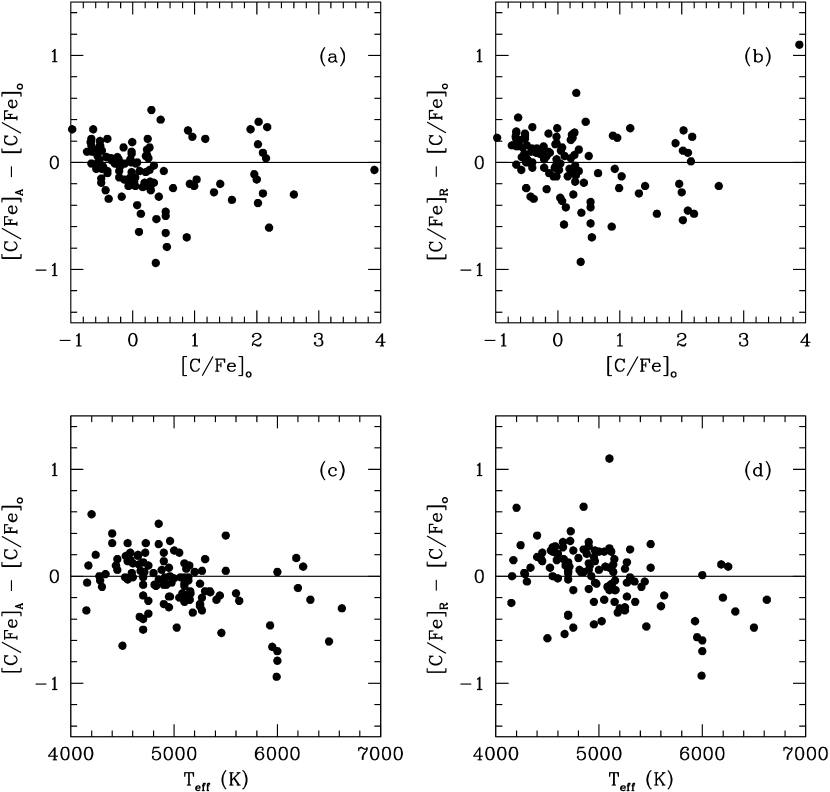
Figure 9: (a) Distributions of residuals of the estimated [C/Fe], based on the ANN approach, [C/Fe]_A, as compared to the adopted literature value, [C/Fe]_o, as a function of [C/Fe]_o. (b) The same as in panel (a), but for [Fe/H]_R. (c) Distributions of residuals of the [C/Fe]_A as compared to [C/Fe]${\rm o}$, as a function of T_eff. (d) The same as in panel (c), but for [C/Fe]_R.

Figure 8 shows the residuals in the determination of the estimated [C/Fe], as compared to the individual predictor variables $KP$ and $GP$, for both the ANN and regression approaches. As can be seen from inspection of this Figure, the residuals are distributed similarly over the predictor variables for both techniques. Some of the largest negative residuals in the estimates of [C/Fe] occur when $KP$ is large, due to the approaching saturation of this index. For both approaches there is a tendency to underestimate [C/Fe] by about 0.5 dex for stars with $GP>6$ Å, as this index approaches saturation. Figure 9 shows the same sets of residuals as a function of the adopted literature values of [C/Fe] and T_eff. Note that both the ANN and regression methods exhibit some of their largest negative residuals between $0<{\rm[C/Fe]}<+1.0$, although there are many smaller residuals in this range as well. In the case of the regression technique, the largest positive residual seen in panels (b) and (d) is associated with HE 0107-5240, where once more the regression approach is failing at this extreme value of [C/Fe]. There are a number of large negative residuals seen in panels (c) and (d) at T${}_{\rm eff}>6000$ K, where the strength of the $GP$ index is rapidly declining due to its sensitivity to temperature, and hence is subject to more measurement error.

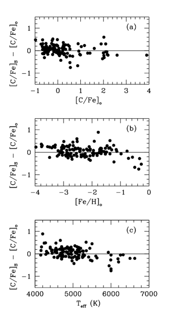
Figure 10: (a) Distributions of residuals of the estimated [C/Fe], based on the synthesis approach, [C/Fe]_S, as compared to the adopted literature value, [C/Fe]_o, as a function of [C/Fe]_o. (b) The same as in panel (a), but as a function of the adopted literature value of [Fe/H]_o. (c) The same as in panel (a), but as a function of T_eff.

Figure 10 shows the residuals in the estimate of [C/Fe] obtained from the spectral synthesis method as a function of the adopted literature values of [C/Fe], [Fe/H], and T_eff, respectively. Note that some of the largest negative residuals in panel (a) occur in the same range of [C/Fe]_o that proved problematic for the ANN and regression estimates. One might be suspicious of the adopted literature values of [C/Fe] for these stars. In panel (b) it is clear that the synthesis estimates of [C/Fe] also appear to exhibit larger negative residuals at higher metallicity, as was seen for the ANN and regression estimates. As was also seen previously, in panel (c) a few of the largest negative residuals occur for T${}_{\rm eff}>6000$, presumably due to the weakness of the G-band, and the difficulty of matching its strength to the models when it is quite small.

Figure 11 (a) shows how the ANN estimates of [C/Fe] for the calibration stars compare with those obtained from the synthesis approach over the entire calibration space. Figure 11 (b) is the residual of the ANN estimate as compared to the synthesis estimate, as a function of the synthesis estimate. With the exception of a number of individual cases near the solar value, and one star with [C/Fe]${}_{\rm S}\simeq+2.6$, the agreement is quite satisfying, at least given the very different methodology applied.

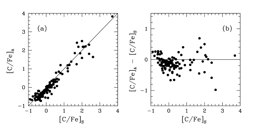
Figure 11: (a) Comparison of the estimated [C/Fe] from the ANN approach, [C/Fe]_A, with that obtained from the synthesis approach, [C/Fe]_S, for the calibration stars. The solid line is the one-to-one relation. (b) Residuals about the one-to-one line as a function of [C/Fe]_S.

We now consider quantitative estimates of the global accuracies obtained, as compared to the adopted literature values for [Fe/H] and [C/Fe] listed in the end notes of Table 4. The results are provided in Table 5. Columns (2)-(6) indicate the mean offset of the estimate under consideration with respect to the adopted literature values. The quantities in parentheses indicate the standard deviation of the estimates about the listed mean offset. We have also explored the accuracy of our derived estimates of [Fe/H] and [C/Fe] over the bins listed in Table 4. Column (1) of Table 5 lists results for the various bins in T${\rm eff}$, [Fe/H], and [C/Fe].

As can be seen from inspection of Table 5, estimates of [Fe/H] from either the ANN or regression approach exhibit similar offsets and scatter. It should be noted that the offsets in the estimates of [Fe/H] for the stars with literature values [Fe/H] $>-1.0$ are low by on the order of 0.3 to 0.4 dex, most likely due to the saturation or near saturation of the $KP$ index. Similarly, and presumably for the same reason, the estimates of [C/Fe] are generally offset by 0.4 to 0.5 dex for the ANN and regression approaches for stars with [Fe/H] $>-1.0$. Interestingly, the synthesis estimates of [C/Fe] suffer from an offset of 0.3 dex for the more metal-rich stars as well.

Other than the obvious problems with the results for the more metal-rich stars, inspection of Table 5 indicates that the ANN and regression estimates of [C/Fe] are only slightly worse than obtained from the synthesis results. There are certainly individual cases, for stars with very strong molecular bands, where one must be concerned about the results obtained from the line-index approach. For such stars there is reason to prefer the synthesis approach for estimation of [C/Fe]. Further discussion of this point is made below.

4 The “Strong G-Band” Stars of Beers, Preston, & Shectman

The HK objective-prism/interference-filter survey of Beers and colleagues has discovered numerous carbon-rich stars over a wide range of metal abundance, extending down to the lowest abundance stars presently known. In a previous paper, BPSII noted 56 stars from their survey with possibly strong G-bands relative to other metal-deficient stars of similar colors. These stars, listed in Table 8 of BPSII, form our program sample. For many of these stars the original spectra that were available (from the original HK survey observations) were not of uniformly high quality (and in some cases were limited in the spectral range covered) to perform a satisfactory analysis, so we obtained additional higher signal-to-noise spectra for the majority of them, using the same telescopes and spectrographs that were employed for the calibration objects. A number of the BPSII “strong G-band stars” have been observed subsequently at higher spectral resolution (indeed, several appear among our calibration objects), which provides an additional check on our ability to estimate metallicities and carbon abundances from medium-resolution spectra of CEMP stars.

Photometric information for our program stars is supplied in Table 6. The column definitions, as well as procedures used to obtain the information listed, are identical to those described for the calibration stars listed in Table 1. One star, CS 30493-064, was not found in the 2MASS catalog, hence we have no $(J-K)_{0}$ for it, and therefore cannot obtain estimates of [Fe/H] for this object.

4.1 Determination of [Fe/H] and [C/Fe] for Program Stars

Table 7 reports our determinations of [Fe/H] and [C/Fe] for the BPSII “strong G-band” stars, using the methods described above. Column (1) lists the star name. In column (2) we list the telescopes involved with the acquisition of the medium-resolution spectra, using the same coding as in Table 3. The $KP$ and $GP$ line indices are listed in columns (3) and (4), respectively. Columns (5) and (6) list estimates of [Fe/H], obtained using the ANNs and regression procedures described above, respectively. Columns (7) and (8) list estimates of [C/Fe], obtained with the ANNs and regression procedures described above, respectively. The remaining columns are described below.

4.2 Spectral Synthesis Calculations for Program Stars

We have used the procedures described above to obtain spectral synthesis estimates of [C/Fe] for all but one of our program stars. In order to obtain these estimates, we require input model atmosphere parameters, estimated in the following manner. Temperatures, which we wish to be on the same scale as the calibration stars, are obtained from a simple linear regression of T_eff with $(J-K)_{0}$, using the adopted temperatures of the atmospheric models of the calibration stars:

$${\rm T}_{\rm eff}=6861\;(56)-3504\;(102)\;(J-K)_{0}$$

$$\epsilon=150~{}K,\;\;\;{\rm R}^{2}=0.91$$

where the one-sigma estimates of the coefficients are indicated in parentheses.

Surface gravities are obtained in a similar manner, relying on the adopted gravities of the calibration objects:

$$\log g=5.232\;(0.190)-6.091\;(0.347)\;(J-K)_{0}$$

$$\epsilon=0.51~{}dex,\;\;\;{\rm R}^{2}=0.71$$

Metallicity estimates are taken to be equal to the ANN estimate, [Fe/H]_A. Microturbulance estimates are all set to $\xi=2.0$ km/s. The full set of adopted parameters for each program star are listed in column (9) of Table 7.

The resulting spectral synthesis estimates of [C/Fe] are listed in column (10) of Table 7. Above we noted that some stars exhibit such strong CH features (generally among the cooler stars) that they compromise the sidebands used for estimation of the $GP$ index; we have indicated these potentially problematic stars with double colons after the estimate of [C/Fe] in columns (7) and (8) of Table 7. Also, as above, stars where either the poor quality of the spectrum or the lack of fit from the synthesis approach led to doubts in the resulting estimate of [C/Fe]_S are indicated with single or double colons next to the listed estimate of [C/Fe]_S.

Column (11) of Table 7 lists our final adopted [C/Fe] determinations for the program stars, [C/Fe]_F. In most cases, this is taken to be a straight average of the reported [C/Fe]_A and [C/Fe]_S values. For cases where we have concerns about the line-index estimates of [C/Fe], we adopt the spectral synthesis estimates of [C/Fe].

5 The Distribution of Carbon Abundances for Low-Metallicity Stars

In Figures 12(a) and 12(b) we show the adopted estimates of [C/Fe] and [C/H] vs. [Fe/H], respectively, for the “strong G-band” stars of BPSII. This Figure is quite similar to that obtained by Rossi et al. (1999), but now is based on much firmer estimates of [Fe/H], [C/Fe], and [C/H]. As is clear from inspection of this Figure, the stars with [Fe/H] $>-1.0$ are not in fact carbon-enhanced, although they were flagged as possible cases in BPSII. The selection of the possibly carbon-enhanced stars from BPSII was based on a comparison of the “strong G-band” candidates with the median G-band strengths of the stars contained in a course grid of [Fe/H] and $B-V$. It appears that this selection was flawed in the high-metallicity regions.

The envelope of [C/Fe] clearly becomes more extreme for the stars with the lowest [Fe/H]. However, as is seen in Figure 12 (b), the upper envelope of [C/H], even at low [Fe/H], reaches a maximum value of [C/H] $\approx-0.5$. As mentioned in the introduction, a number of different astrophysical phenomena are likely to be responsible for the enhancement of carbon at low metallicity. It is interesting that, independent of [Fe/H], the maximum level of [C/H] that is obtained is remarkably constant. If all of the CEMP stars obtained their carbon enhancement as the result of the transfer of AGB-processed material from a now-deceased companion, this result places a strong constraint on the level of carbon enhancement that must be accounted for by models of AGB evolution at low metallicity. However, we suspect that it may not be the case that all of the CEMP stars can be accounted for by this single process. It is worth noting that, for metallicities in the range [Fe/H] $<-2.5$, the distribution of [C/H] for CEMP stars may be bi-modal, which also suggests that several nucleosynthetic processes may be involved.

Figure 12: Final estimates of the carbon ratios [C/Fe]_F and [C/H]_F, for the program stars from BPSII, as a function of the ANN estimate of metallicity [Fe/H]_A.

6 Summary and Discussion

We have described procedures for the estimation of [Fe/H] and [C/Fe] for stars in the range of abundance $-5.5\leq{\rm[Fe/H]}\leq-1.0$, and with near-infrared colors in the range $0.2\leq(J-K)_{0}\leq 0.8$. The ANN and regression approaches exhibit similar errors, although they are slightly worse than obtained from the spectral synthesis technique. For stars that are either very cool, or have very large [C/Fe], the synthesis approach is to be preferred, because of the contamination of the sidebands of the $GP$ index by molecular carbon lines.

It is our intention to apply these methods to the determination of [Fe/H] and [C/Fe] for the large numbers of CEMP stars identified in the HK survey, the HES, in the sample of C-rich stars identified by Christlieb et al. (2001), and for carbon-enhanced stars found in SDSS and SEGUE. It may be necessary to recalibrate some of our estimates of [Fe/H] and [C/Fe] for stars with extremely strong carbon lines, as well as to better populate the calibration space with stars of known [Fe/H] and [C/Fe]. This might be accomplished in two ways, either by including additional stars into the calibrations or by calibrating to a grid of carbon-enhanced models. Both avenues are presently being pursued. Once this is accomplished, a more quantitative estimate of the frequency of CEMP stars as a function of [Fe/H] will be obtained. This is of clear importance, since the quoted frequencies of CEMP stars in the literature are based on preliminary calibrations, and/or partial spectroscopic follow-up. Additional samples for the investigation of this question are now available from the medium-resolution stellar spectra obtained during the course of the SDSS; these are presently being analyzed. The extension of the SDSS, in particular SEGUE, will no doubt identify many additional CEMP stars, which will be examined in due course.

Table 1: Photometric Information for Calibration Stars

Star	$V$	$(B-V)$	$J$	$J-K$	$E(B-V)_{A}$	$(B-V)_{0}$	$(J-K)_{0}$
(1)	(2)	(3)	(4)	(5)	(6)	(7)	(8)
BD$+$06:648	9.10	1.11	6.562 (0.020)	0.764 (0.027)	0.207	0.90	0.648
BD$+$09:2870	9.70	0.88	7.534 (0.020)	0.665 (0.030)	0.029	0.85	0.649
BD$+$09:3223	9.25	0.56	7.760 (0.020)	0.483 (0.030)	0.076	0.48	0.440
BD$+$17:3248	9.37	0.66	7.876 (0.056)	0.538 (0.059)	0.059	0.60	0.505
BD$+$30:2611	9.13	1.15	6.882 (0.023)	0.788 (0.031)	0.019	1.13	0.777
BD$+$34:2476	10.06	0.38	9.077 (0.019)	0.266 (0.026)	0.014	0.37	0.258
BD$+$37:1458	8.92	0.59	7.532 (0.020)	0.446 (0.027)	0.217	0.37	0.324
BD$-$01:2582	9.60	0.67	8.126 (0.020)	0.528 (0.029)	0.021	0.65	0.516
BD$-$09:5831	9.50	0.83	8.486 (0.020)	0.673 (0.033)	0.041	0.79	0.650
BD$-$18:5550	9.36	0.88	7.202 (0.020)	0.647 (0.027)	0.159	0.72	0.558
CD$-$23:72	9.20	0.58	8.147 (0.021)	0.464 (0.030)	0.020	0.56	0.453
BS 16082–129	13.61	0.62	11.855 (0.022)	0.546 (0.027)	0.000	0.60	0.535
BS 16467–062	14.09	0.60	12.680 (0.022)	0.482 (0.029)	0.000	0.60	0.482
BS 16469–075	13.42	0.77	11.753 (0.022)	0.551 (0.029)	0.000	0.75	0.540
BS 16477–003	14.22	0.72	12.518 (0.027)	0.577 (0.035)	0.000	0.71	0.571
BS 16928–053	13.54	0.84	11.655 (0.021)	0.613 (0.028)	0.000	0.83	0.607
BS 16929–005	13.61	0.62	12.172 (0.022)	0.503 (0.030)	0.000	0.61	0.497
BS 17569–049	13.36	0.89	11.503 (0.024)	0.650 (0.032)	0.000	0.86	0.633
BS 17583–100	12.37	0.51	11.103 (0.029)	0.446 (0.035)	0.000	0.41	0.390
CS 22169–035	12.88	0.91	11.002 (0.024)	0.649 (0.033)	0.042	0.87	0.625
CS 22183–031	13.62	0.62	12.111 (0.026)	0.529 (0.036)	0.000	0.58	0.507
CS 22189–009	13.97	0.76	12.391 (0.021)	0.593 (0.035)	0.024	0.74	0.580
CS 22873–055	12.65	0.93	10.654 (0.024)	0.648 (0.033)	0.077	0.85	0.605
CS 22873–128	13.03	0.69	11.430 (0.029)	0.556 (0.038)	0.040	0.65	0.534
CS 22873–166	11.82	0.99	9.832 (0.024)	0.695 (0.033)	0.044	0.95	0.670
CS 22877–001	12.16	0.77	10.555 (0.024)	0.564 (0.032)	0.054	0.72	0.534
CS 22880–074	13.27	0.57	11.990 (0.023)	0.354 (0.033)	0.057	0.51	0.322
CS 22881–036	13.95	0.47	12.968 (0.026)	0.280 (0.040)	0.013	0.46	0.273
CS 22885–096	13.33	0.69	11.630 (0.024)	0.540 (0.035)	0.055	0.63	0.509
CS 22891–200	13.93	0.84	11.995 (0.022)	0.581 (0.032)	0.078	0.76	0.537
CS 22891–209	12.18	0.85	10.235 (0.024)	0.612 (0.032)	0.072	0.78	0.572
CS 22892–052	13.20	0.79	11.492 (0.021)	0.563 (0.030)	0.032	0.76	0.545
CS 22896–154	13.63	0.64	12.072 (0.026)	0.532 (0.035)	0.053	0.59	0.502
CS 22897–008	13.33	0.69	11.596 (0.026)	0.594 (0.033)	0.031	0.66	0.577
CS 22898–027	12.76	0.50	11.719 (0.022)	0.298 (0.033)	0.065	0.43	0.262
CS 22942–019	12.69	0.88	11.193 (0.028)	0.548 (0.035)	0.019	0.86	0.537
CS 22947–187	12.99	0.64	11.468 (0.024)	0.440 (0.032)	0.069	0.57	0.401
CS 22948–027	12.66	1.13	10.979 (0.024)	0.552 (0.033)	0.026	1.10	0.537
CS 22948–066	13.47	0.63	11.966 (0.023)	0.525 (0.034)	0.025	0.60	0.511
CS 22949–037	14.36	0.76	12.650 (0.024)	0.575 (0.034)	0.052	0.71	0.546
CS 22949–048	13.67	0.81	11.919 (0.023)	0.637 (0.033)	0.036	0.77	0.617
CS 22953–003	13.75	0.68	12.173 (0.022)	0.531 (0.033)	0.018	0.66	0.521
CS 22957–027	13.60	0.79	12.092 (0.028)	0.483 (0.037)	0.039	0.75	0.461
CS 22968–014	13.70	0.74	12.026 (0.024)	0.559 (0.035)	0.012	0.73	0.552
CS 29495–041	13.34	0.81	11.607 (0.024)	0.583 (0.033)	0.000	0.81	0.583
CS 29498–043	13.72	1.08	11.621 (0.023)	0.683 (0.032)	0.103	0.98	0.625
CS 29502–042	12.74	0.66	11.150 (0.023)	0.497 (0.033)	0.000	0.66	0.497
CS 29502–092	11.87	0.77	10.177 (0.027)	0.576 (0.033)	0.099	0.67	0.521
CS 29516–024	13.57	0.86	11.636 (0.026)	0.663 (0.033)	0.000	0.80	0.629
CS 29518–051	13.02	0.60	11.540 (0.024)	0.508 (0.034)	0.000	0.60	0.508
CS 29526–110	13.35	0.36	12.587 (0.026)	0.220 (0.035)	0.023	0.34	0.207
CS 30301–015	13.04	1.00	11.304 (0.020)	0.566 (0.030)	0.049	0.95	0.539
CS 30306–132	12.73	0.89	11.302 (0.024)	0.551 (0.033)	0.000	0.88	0.545
CS 30314–067	11.85	1.13	9.759 (0.024)	0.731 (0.031)	0.068	1.06	0.693
CS 30325–094	12.32	0.70	10.661 (0.021)	0.538 (0.030)	0.000	0.68	0.527
CS 31062–012	12.10	0.47	11.046 (0.021)	0.275 (0.028)	0.019	0.45	0.264
CS 31062–050	13.05	0.65	11.765 (0.021)	0.360 (0.031)	0.030	0.62	0.343
CS 31082–001	11.67	0.77	10.053 (0.024)	0.589 (0.031)	0.015	0.76	0.581
HD 97	9.40	0.64	8.057 (0.019)	0.544 (0.029)	0.021	0.62	0.532
HD 2665	7.75	0.71	6.026 (0.024)	0.552 (0.029)	0.289	0.42	0.390
HD 2796	8.52	0.70	6.853 (0.020)	0.597 (0.026)	0.020	0.68	0.586
HD 3008	9.70	1.14	7.181 (0.018)	0.764 (0.025)	0.030	1.11	0.747
HD 4306	9.05	0.70	7.424 (0.025)	0.601 (0.033)	0.036	0.66	0.581
HD 4395	7.70	0.69	6.394 (0.023)	0.422 (0.029)	0.026	0.66	0.407
HD 5426	9.63	0.63	8.082 (0.034)	0.534 (0.043)	0.016	0.61	0.525
HD 6268	8.16	0.78	6.335 (0.020)	0.621 (0.027)	0.017	0.76	0.611
HD 6755	7.73	0.60	6.197 (0.024)	0.535 (0.029)	0.000	0.60	0.535
HD 26169	8.79	0.74	7.172 (0.029)	0.538 (0.042)	0.079	0.66	0.494
HD 26297	7.47	1.02	5.379 (0.018)	0.748 (0.027)	0.031	0.99	0.731
HD 44007	8.06	0.79	6.340 (0.020)	0.637 (0.031)	0.186	0.60	0.533
HD 45282	8.02	0.66	6.591 (0.020)	0.502 (0.028)	0.000	0.66	0.502
HD 74462	8.74	0.85	6.688 (0.027)	0.641 (0.040)	0.053	0.80	0.611
HD 83212	8.28	0.99	6.307 (0.021)	0.698 (0.030)	0.055	0.93	0.667
HD 85773	9.39	1.10	7.230 (0.024)	0.725 (0.032)	0.046	1.05	0.699
HD 87140	8.98	0.70	7.471 (0.025)	0.528 (0.030)	0.006	0.69	0.525
HD 88446	7.90	0.54	6.771 (0.027)	0.319 (0.037)	0.034	0.51	0.300
HD 88609	8.59	0.93	6.665 (0.029)	0.659 (0.034)	0.000	0.93	0.659
HD 89948	7.51	0.46	6.498 (0.027)	0.309 (0.036)	0.063	0.40	0.274
HD 93529	9.30	0.75	7.503 (0.027)	0.630 (0.032)	0.077	0.67	0.587
HD 103036	8.18	1.29	5.860 (0.020)	0.814 (0.029)	0.028	1.26	0.798
HD 103545	9.20	0.71	7.608 (0.021)	0.620 (0.036)	0.035	0.67	0.600
HD 105546	8.61	0.79	7.152 (0.025)	0.478 (0.031)	0.021	0.77	0.466
HD 105740	8.38	0.94	6.506 (0.018)	0.659 (0.030)	0.041	0.90	0.636
HD 108317	8.30	0.55	6.623 (0.025)	0.470 (0.033)	0.017	0.53	0.460
HD 108577	9.60	0.63	7.995 (0.024)	0.532 (0.039)	0.026	0.60	0.517
HD 110184	8.27	1.14	6.125 (0.024)	0.779 (0.035)	0.022	1.12	0.767
HD 111721	7.97	0.79	6.347 (0.019)	0.561 (0.025)	0.054	0.74	0.531
HD 115444	8.97	0.78	7.160 (0.019)	0.553 (0.028)	0.000	0.78	0.553
HD 118055	8.86	1.29	6.573 (0.020)	0.849 (0.028)	0.093	1.20	0.797
HD 121135	9.30	0.60	7.750 (0.018)	0.568 (0.028)	0.027	0.57	0.553
HD 122956	7.22	0.95	5.230 (0.020)	0.667 (0.029)	0.084	0.87	0.620
HD 123585	9.27	0.52	8.349 (0.032)	0.268 (0.040)	0.096	0.42	0.214
HD 126238	7.66	0.81	5.975 (0.019)	0.637 (0.025)	0.114	0.70	0.573
HD 126587	9.17	0.80	7.258 (0.020)	0.590 (0.028)	0.097	0.70	0.536
HD 128279	8.09	0.60	6.568 (0.019)	0.503 (0.028)	0.099	0.50	0.448
HD 135148	9.40	1.21	7.137 (0.030)	0.769 (0.037)	0.036	1.17	0.749
HD 136316	7.62	1.21	5.354 (0.018)	0.807 (0.028)	0.000	1.21	0.807
HD 140283	7.23	0.49	6.014 (0.019)	0.426 (0.025)	0.140	0.35	0.348
HD 141531	9.15	1.15	6.971 (0.027)	0.756 (0.034)	0.049	1.10	0.729
HD 142948	8.03	0.93	6.139 (0.023)	0.626 (0.029)	0.050	0.88	0.598
HD 166161	8.16	0.93	5.998 (0.021)	0.654 (0.033)	0.000	0.93	0.654
HD 175305	7.20	0.73	5.613 (0.023)	0.556 (0.030)	0.106	0.62	0.497
HD 178443	10.03	0.67	8.414 (0.018)	0.503 (0.032)	0.090	0.58	0.453
HD 184711	7.98	1.33	5.513 (0.024)	0.805 (0.029)	0.136	1.19	0.729
HD 186478	8.92	0.91	7.117 (0.023)	0.674 (0.029)	0.112	0.80	0.611
HD 187111	7.72	1.22	5.366 (0.020)	0.816 (0.027)	0.156	1.06	0.729
HD 196944	8.41	0.61	7.017 (0.023)	0.487 (0.029)	0.041	0.57	0.464
HD 200654	9.16	0.60	7.648 (0.018)	0.494 (0.027)	0.028	0.57	0.478
HD 204543	8.60	0.76	6.462 (0.023)	0.685 (0.028)	0.040	0.72	0.663
HD 206739	8.70	0.89	6.698 (0.021)	0.665 (0.032)	0.053	0.84	0.635
HD 210595	8.60	0.45	7.642 (0.023)	0.243 (0.031)	0.078	0.37	0.199
HD 216143	8.20	0.94	5.871 (0.023)	0.724 (0.031)	0.042	0.90	0.700
HD 218857	8.72	0.67	7.397 (0.019)	0.524 (0.025)	0.036	0.63	0.504
HE 0024–2523	14.91	0.41	14.038 (0.026)	0.289 (0.046)	0.017	0.39	0.279
HE 0107–5240	15.17	0.67	13.676 (0.027)	0.458 (0.043)	0.000	0.66	0.452
LP 625–44	11.85	0.69	10.432 (0.024)	0.393 (0.034)	0.154	0.54	0.307
LP 685–44	11.77	0.63	10.309 (0.029)	0.455 (0.036)	0.276	0.35	0.300
LP 685–47	12.55	0.76	10.686 (0.023)	0.537 (0.032)	0.325	0.43	0.355
LP 706–7	12.13	0.87	11.046 (0.021)	0.275 (0.028)	0.019	0.85	0.264

Table 2: Line Index Wavelength Bands

Line	Line Band	Blue Sideband	Red Sideband
CaII-K6	3930.7 – 3936.7	3903.0 – 3923.0	4000.0 – 4020.0
CaII-K12	3927.7 – 3939.7	3903.0 – 3923.0	4000.0 – 4020.0
CaII-K18	3924.7 – 3942.7	3903.0 – 3923.0	4000.0 – 4020.0
G band ($GP$)	4297.5 – 4312.5	4247.0 – 4267.0	4363.0 – 4372.0

Table 3: Spectroscopic Observations, and Adopted Abundance and Model Parameters for Calibration Stars

Star	Telescope	$~{}KP$	$~{}GP$	[Fe/H]	[C/H]	[C/Fe]	Source	Model Parameters
(1)	(2)	(3)	(4)	(5)	(6)	(7)	(8)	(9)
BD$+$06:648	K	7.28	2.39	$-$2.33	$-$2.23	$+$0.10	12	4500/1.1/-2.3/2.0
BD$+$09:2870	k	7.75	2.91	$-$2.29	$-$2.90	$-$0.61	12	4600/1.4/-2.3/1.7
BD$+$09:3223	k	5.51	1.09	$-$2.19	$-$2.70	$-$0.51	12	5350/2.0/-2.2/2.0
BD$+$17:3248	ck	6.46	1.42	$-$2.07	$-$2.51	$-$0.44	23	5250/1.4/-2.1/1.5
BD$+$30:2611	MPk	10.93	4.61	$-$1.24	$-$1.90	$-$0.66	12	4170/0.4/-1.2/1.6
BD$+$34:2476	k	2.88	0.61	$-$1.98	$-$1.94	$+$0.04	11	6320/3.9/-2.0/1.0
BD$+$37:1458	k	5.74	3.28	$-$1.96	$-$1.73	$+$0.24	11,12	5410/3.6/-2.0/1.0
BD$-$01:2582	Lcek	5.56	6.23	$-$2.19	$-$1.10	$+$0.99	12	5150/2.5/-2.2/1.2
BD$-$09:5831	ck	9.89	4.50	$-$1.73	$-$2.39	$-$0.67	12	4580/1.5/-1.7/1.5
BD$-$18:5550	csk	4.40	2.27	$-$3.06	$-$3.08	$-$0.02	23	4750/1.4/-3.1/1.8
CD$-$23:72	k	8.93	4.26	$-$0.98	$-$1.51	$-$0.53	12	5300/2.6/-1.0/2.0
BS 16082–129	I	4.33	2.09	$-$2.86	$-$2.57	$+$0.29	24	4900/1.8/-2.9/1.6
BS 16467–062	Kk	1.55	0.28	$-$3.77	$-$3.52	$+$0.25	23	5200/2.5/-3.8/1.6
BS 16469–075	I	3.46	1.90	$-$3.03	$-$2.82	$+$0.21	24	4880/2.0/-3.0/1.4
BS 16477–003	ks	2.92	1.49	$-$3.36	$-$3.02	$+$0.34	23	4900/1.7/-3.4/1.8
BS 16928–053	I	4.84	1.89	$-$2.91	$-$3.14	$-$0.23	24	4590/0.9/-2.9/1.6
BS 16929–005	I	2.80	2.20	$-$3.09	$-$2.17	$+$0.92	24	5270/2.7/-3.1/1.3
BS 17569–049	I	5.90	2.33	$-$2.88	$-$3.10	$-$0.22	23	4700/1.2/-2.9/1.9
BS 17583–100	I	2.63	0.83	$-$2.42	$-$1.89	$+$0.53	24	5930/4.0/-2.4/1.4
CS 22169–035	P	4.43	2.37	$-$3.04	$-$2.76	$+$0.28	23	4700/1.2/-3.0/2.2
CS 22183–031	P	3.17	1.31	$-$2.93	$-$2.51	$+$0.42	24	5270/2.8/-2.9/1.2
CS 22189–009	ELes	2.41	1.19	$-$3.49	$-$3.22	$+$0.27	23	4900/1.7/-3.5/1.9
CS 22873–055	L	5.77	1.18	$-$2.99	$-$3.97	$-$0.98	23	4550/0.7/-3.0/2.2
CS 22873–128	Le	4.07	1.97	$-$2.88	$-$2.81	$+$0.07	4	4960/2.1/-2.9/1.9
CS 22873–166	L	5.81	3.24	$-$2.97	$-$3.12	$-$0.15	23	4550/0.9/-3.0/2.1
CS 22877–001	Lcks	3.43	4.57	$-$2.77	$-$1.36	$+$1.41	15,18	5050/1.9/-2.8/2.2
CS 22880–074	Le	3.43	5.70	$-$1.85	$-$0.44	$+$1.41	16,19	5950/3.9/-1.9/1.7
CS 22881–036	Lce	2.55	5.33	$-$2.06	$-$0.10	$+$1.96	16	6200/4.0/-2.1/2.2
CS 22885–096	Ls	1.70	0.60	$-$3.78	$-$3.54	$+$0.24	23	5050/2.6/-3.8/1.8
CS 22891–200	L	3.87	1.71	$-$3.49	$-$2.96	$+$0.53	4	4700/1.0/-3.5/2.2
CS 22891–209	Le	3.88	0.83	$-$3.29	$-$3.81	$-$0.52	23	4700/1.0/-3.3/2.1
CS 22892–052	Peks	4.03	5.64	$-$3.03	$-$2.14	$+$0.89	23	4850/1.6/-3.0/1.9
CS 22896–154	L	4.27	2.48	$-$2.69	$-$2.42	$+$0.27	23	5250/2.7/-2.7/1.2
CS 22897–008	Ls	3.48	2.27	$-$3.41	$-$2.91	$+$0.50	23	4900/1.7/-3.4/2.0
CS 22898–027	Pes	1.84	4.66	$-$2.25	$-$0.24	$+$2.02	4,16,19	6180/3.8/-2.3/1.6
CS 22942–019	Le	3.41	7.63	$-$2.66	$-$0.56	$+$2.10	16,19	4950/2.1/-2.7/2.1
CS 22947–187	Les	4.16	4.51	$-$2.49	$-$1.46	$+$1.03	4	5160/1.3/-2.5/2.3
CS 22948–027	Le	3.86	7.82	$-$2.53	$-$0.51	$+$2.02	13,16,18	4670/1.2/-2.5/2.0
CS 22948–066	L	2.86	0.71	$-$3.14	$-$3.16	$-$0.02	23	5100/1.8/-3.1/2.0
CS 22949–037	P	1.75	2.05	$-$3.97	$-$2.80	$+$1.17	23	4900/1.5/-4.0/1.8
CS 22949–048	P	3.59	1.29	$-$3.17	$-$3.01	$+$0.16	4	4750/1.1/-3.2/2.3
CS 22953–003	Les	3.70	2.47	$-$2.84	$-$2.19	$+$0.65	23	5100/2.3/-2.8/1.7
CS 22957–027	Pe	2.01	7.44	$-$3.22	$-$1.05	$+$2.17	7,9,16,20	4960/2.1/-3.2/1.6
CS 22968–014	EL	1.98	1.35	$-$3.56	$-$3.26	$+$0.30	23	4850/1.7/-3.6/1.9
CS 29495–041	L	4.98	2.52	$-$2.82	$-$2.86	$-$0.04	23	4800/1.5/-2.8/1.8
CS 29498–043	ks	2.38	6.85	$-$3.75	$-$1.85	$+$1.90	20	4400/0.6/-3.8/2.3
CS 29502–042	e	2.83	1.47	$-$3.19	$-$2.96	$+$0.23	23	5100/2.5/-3.2/1.5
CS 29502–092	s	3.41	4.51	$-$2.76	$-$1.80	$+$0.96	18	5000/2.1/-2.8/1.8
CS 29516–024	e	4.89	3.02	$-$3.07	$-$3.08	$-$0.01	23	4650/1.2/-3.1/1.7
CS 29518–051	e	4.63	1.54	$-$2.78	$-$3.05	$-$0.27	23	5100/2.4/-2.8/1.4
CS 29526–110	s	1.23	1.47	$-$2.38	$-$0.18	$+$2.20	19	6500/3.2/-2.4/1.6
CS 30301–015	k	4.96	7.88	$-$2.64	$-$1.04	$+$1.60	19	4750/0.8/-2.6/2.2
CS 30306–132	s	5.62	3.63	$-$2.42	$-$2.08	$+$0.34	24	5110/2.5/-2.4/1.8
CS 30314–067	s	5.05	5.80	$-$2.85	$-$2.40	$+$0.45	18	4400/0.7/-2.9/2.5
CS 30325–094	k	3.10	1.17	$-$3.30	$-$3.32	$-$0.02	23	4950/2.0/-3.3/1.5
CS 31062–012	s	1.54	3.67	$-$2.55	$-$0.45	$+$2.10	19	6250/4.5/-2.6/1.5
CS 31062–050	s	2.94	6.42	$-$2.32	$-$0.32	$+$2.00	19	5600/3.0/-2.3/1.3
CS 31082–001	Ake	4.91	2.84	$-$2.89	$-$2.68	$+$0.21	23	4830/1.5/-2.9/1.8
HD 97	Lks	9.98	5.12	$-$1.23	$-$1.10	$+$0.13	12	5030/2.6/-1.2/1.2
HD 2665	k	7.45	4.11	$-$1.95	$-$2.08	$-$0.13	12	5060/2.4/-2.0/1.5
HD 2796	Lceks	6.37	1.40	$-$2.47	$-$2.98	$-$0.51	23	4950/1.5/-2.5/2.1
HD 3008	ck	9.90	4.27	$-$1.92	$-$2.10	$-$0.18	12	4150/0.6/-1.9/2.2
HD 4306	Lcks	4.89	2.57	$-$2.89	$-$2.78	$+$0.11	24	4810/1.8/-2.9/1.6
HD 4395	c	9.22	5.61	$-$0.33	$+$0.05	$+$0.38	3	5460/3.3/-0.3/1.3
HD 5426	ce	6.94	3.62	$-$2.41	$-$2.56	$-$0.15	4	4910/1.9/-2.4/2.2
HD 6268	k	6.75	1.65	$-$2.63	$-$3.30	$-$0.67	24	4600/1.0/-2.6/2.1
HD 6755	k	8.51	4.31	$-$1.53	$-$1.60	$-$0.07	12	5150/2.7/-1.5/1.4
HD 26169	s	5.94	3.55	$-$2.30	$-$2.25	$+$0.05	12	5140/2.6/-2.3/1.4
HD 26297	ks	10.47	4.60	$-$1.67	$-$2.34	$-$0.67	12	4450/1.2/-1.7/1.6
HD 44007	KLks	9.23	5.06	$-$1.70	$-$1.92	$-$0.22	8	4850/2.0/-1.7/1.5
HD 45282	Keks	8.65	4.09	$-$1.37	$-$1.59	$-$0.22	12	5340/3.0/-1.4/1.2
HD 74462	ko	10.73	5.48	$-$1.37	$-$1.87	$-$0.50	12	4660/1.6/-1.4/1.4
HD 83212	Kks	10.76	4.91	$-$1.41	$-$2.09	$-$0.68	12	4530/1.5/-1.4/1.8
HD 85773	KLk	7.66	2.76	$-$2.43	$-$3.00	$-$0.57	12	4450/1.1/-2.4/2.1
HD 87140	k	7.79	4.25	$-$1.68	$-$1.72	$-$0.04	11,12	5160/3.0/-1.7/1.3
HD 88446	Lc	8.16	4.28	$-$0.36	$-$0.19	$+$0.55	3	6000/4.5/-0.4/0.9
HD 88609	k	5.91	1.63	$-$3.07	$-$3.58	$-$0.51	24	4550/1.1/-3.1/2.4
HD 89948	Lc	7.90	4.57	$-$0.27	$+$0.26	$+$0.53	3	5950/4.1/-0.3/0.8
HD 93529	ks	9.98	5.27	$-$1.37	$-$1.90	$-$0.53	12	4650/1.7/-1.4/1.4
HD 103036	Lk	10.42	4.56	$-$1.78	$-$2.87	$-$1.09	8	4200/0.1/-1.8/2.8
HD 103545	k	7.43	3.33	$-$2.06	$-$2.70	$-$0.64	12	4730/1.7/-2.1/1.3
HD 105546	k	9.20	3.17	$-$1.47	$-$2.21	$-$0.74	12	5150/2.5/-1.5/1.6
HD 105740	k	11.04	6.07	$-$0.58	$-$0.51	$+$0.07	5	4700/2.5/-0.6/1.0
HD 108317	PLk	5.42	2.62	$-$2.24	$-$2.20	$+$0.04	12	5300/2.9/-2.2/1.0
HD 108577	Pck	6.44	1.58	$-$2.11	$-$2.70	$-$0.59	12	4980/1.7/-2.1/1.9
HD 110184	Lk	8.82	3.70	$-$2.52	$-$3.19	$-$0.67	24	4240/0.3/-2.5/2.1
HD 111721	s	9.88	5.32	$-$1.13	$-$1.26	$-$0.14	11,12	5080/2.9/-1.1/1.2
HD 115444	k	4.70	1.80	$-$2.85	$-$3.26	$-$0.41	24	4720/1.5/-2.9/1.7
HD 118055	ek	10.40	4.50	$-$1.75	$-$2.23	$-$0.48	12	4280/1.1/-1.8/1.5
HD 121135	k	9.46	4.04	$-$1.49	$-$1.90	$-$0.41	12	4930/1.5/-1.5/2.0
HD 122956	CLcks	10.15	5.10	$-$1.70	$-$2.23	$-$0.53	11,12	4580/1.4/-1.7/1.7
HD 123585	c	5.90	3.97	$-$0.50	$+$0.37	$+$0.87	1	6000/3.5/-0.5/2.3
HD 126238	Lcs	8.58	4.77	$-$1.53	$-$1.71	$-$0.18	11,12	5000/2.5/-1.5/1.5
HD 126587	L	5.31	2.84	$-$2.78	$-$2.59	$+$0.19	24	4960/2.1/-2.8/1.8
HD 128279	CKLs	6.17	2.78	$-$2.10	$-$2.15	$-$0.05	4,12	5440/3.1/-2.1/1.8
HD 135148	LPck	9.66	6.79	$-$1.92	$-$1.94	$-$0.02	12	4280/0.8/-1.9/2.1
HD 136316	es	10.41	4.44	$-$1.73	$-$2.36	$-$0.63	11,12	4440/1.2/-1.7/1.9
HD 140283	AILPekos	2.75	0.89	$-$2.53	$-$2.25	$+$0.28	24	5630/3.5/-2.5/1.4
HD 141531	K	10.84	4.82	$-$1.63	$-$2.17	$-$0.54	12	4340/1.1/-1.6/1.5
HD 142948	cs	10.53	5.80	$-$0.77	$-$1.12	$-$0.35	12	4710/2.2/-0.8/1.4
HD 166161	Lk	9.05	4.32	$-$1.15	$-$1.57	$-$0.42	12	5270/2.5/-1.2/1.6
HD 175305	M	9.11	5.00	$-$1.31	$-$1.52	$-$0.21	12	5140/2.9/-1.3/1.3
HD 178443	es	7.68	1.96	$-$2.07	$-$2.46	$-$0.39	4	5180/1.7/-2.1/2.6
HD 184711	CLs	7.68	2.56	$-$2.56	$-$3.06	$-$0.50	11	4160/0.2/-2.6/2.5
HD 186478	Kck	7.17	3.18	$-$2.59	$-$2.93	$-$0.34	23	4700/1.3/-2.6/2.0
HD 187111	k	11.04	5.00	$-$1.69	$-$2.10	$-$0.41	11,12	4300/0.6/-1.7/1.9
HD 196944	ck	4.09	5.06	$-$2.38	$-$1.07	$+$1.31	10,17,19	5250/1.6/-2.4/1.9
HD 200654	es	3.43	1.95	$-$2.99	$-$2.76	$+$0.23	2,4	5120/2.6/-3.0/1.4
HD 204543	k	9.81	3.74	$-$1.82	$-$2.40	$-$0.58	12	4700/1.7/-1.8/2.0
HD 206739	ck	10.65	5.45	$-$1.57	$-$2.00	$-$0.43	12	4680/1.7/-1.6/1.7
HD 210595	c	5.81	1.48	$-$0.72	$-$0.35	$+$0.37	11	5990/2.8/-0.7/1.4
HD 216143	ck	8.29	4.08	$-$2.15	$-$2.44	$-$0.29	12	4530/0.8/-2.2/1.8
HD 218857	KLck	7.11	3.78	$-$1.82	$-$1.80	$+$0.02	12	5130/2.4/-1.8/1.2
HE 0024–2523	Mcs	1.03	2.32	$-$2.72	$-$0.12	$+$2.60	22	6630/4.3/-2.7/1.4
HE 0107–5240	As	0.29	5.43	$-$5.30	$-$1.40	$+$3.90	21	5100/2.2/-5.3/2.2
LP 625–44	es	1.86	5.99	$-$2.70	$-$0.71	$+$2.03	6,14	5500/2.8/-2.7/1.3
LP 685–44	es	3.60	1.03	$-$2.67	$-$2.92	$-$0.25	2	5500/3.2/-2.7/1.0
LP 685–47	ks	3.58	0.67	$-$2.79	$-$3.04	$-$0.25	2	5300/2.5/-2.8/1.0
LP 706–7	Ac	1.69	4.18	$-$2.74	$-$0.59	$+$2.15	6,14	6000/3.8/-2.7/1.3

Note. — Telescope translation codes: A = Anglo Australian 3.8m telescope; C = CTIO 4m telescope; K = KPNO 4m telescope; I = Isaac Newton 2.5m telescope; L = Las Campanas 2.5m telescope; M = McDonald Observatory 2.7m telescope; P = Palomar 5m telescope; c = CTIO 1.5m telescope; e = ESO 1.5m telescope; k = KPNO 2.1m telescope; s = SSO 2.3m telescope

References. — 1 = Luck & Bond (1991); 2 = Ryan et al. (1991); 3 = Smith, Coleman, & Lambert (1993); 4 = McWilliam et al. (1995); 5 = Shetrone (1996); 6 = Norris et al. (1997a); 7 = Norris et al. (1997b); 8 = Pilachowski et al. (1997); 9 = Bonifacio et al. (1998); 10 = Zacs et al. (1998); 11 = Carretta et al. (2000); 12 = Gratton et al. (2000); 13 = Hill et al. (2000); 14 = Aoki et al. (2001); 15 = Giridhar et al. (2001); 16 = Preston & Sneden (2001); 17 = Van Eck et al. (2001); 18 = Aoki et al. (2002a); 19 = Aoki et al. (2002b); 20 = Aoki et al. (2002c); 21 = Christlieb et al. (2002); 22 = Lucatello et al. (2003); 23 = Depagne et al. (2002), Cayrel et al. (2004), Spite et al. (2005); 24 = Honda et al. (2004)

Table 4: Estimates of [Fe/H] and [C/Fe] from ANNs, Regression, and Synthesis for Calibration Stars

Star	[Fe/H]	[Fe/H]A	[Fe/H]R	[C/Fe]	[C/Fe]A	[C/Fe]R	Bins	[C/Fe]S	Notes
(1)	(2)	(3)	(4)	(5)	(6)	(7)	(8)	(9)	(10)
BD$+$06:648	$-$2.33	$-$2.39 ($-$0.06)	$-$2.34 ($-$0.01)	$+$0.10	$-$0.55 ($-$0.65)	$-$0.48 ($-$0.58)	4/3/3	$-$0.05 ($-$0.15)	X
BD$+$09:2870	$-$2.29	$-$2.25 ($+$0.04)	$-$2.20 ($+$0.09)	$-$0.61	$-$0.49 ($+$0.12)	$-$0.40 ($+$0.21)	3/3/4	$-$0.75 ($-$0.14)
BD$+$09:3223	$-$2.19	$-$2.21 ($-$0.02)	$-$2.06 ($+$0.13)	$-$0.51	$-$0.66 ($-$0.15)	$-$0.75 ($-$0.24)	2/3/4	$-$0.37: ($+$0.14)
BD$+$17:3248	$-$2.07	$-$2.18 ($-$0.11)	$-$2.02 ($+$0.05)	$-$0.44	$-$0.70 ($-$0.26)	$-$0.76 ($-$0.32)	2/3/4	$-$0.60 ($-$0.16)
BD$+$30:2611	$-$1.24	$-$1.65 ($-$0.41)	$-$1.82 ($-$0.58)	$-$0.66	$-$0.56 ($+$0.10)	$-$0.51 ($+$0.15)	4/2/4	$-$0.35:: ($+$0.31)
BD$+$34:2476	$-$1.98	$-$1.99 ($-$0.01)	$-$2.21 ($-$0.23)	$+$0.04	$-$0.18 ($-$0.22)	$-$0.29 ($-$0.33)	1/2/3	+0.00:: ($-$0.04)
BD$+$37:1458	$-$1.96	$-$1.52 ($+$0.44)	$-$1.52 ($+$0.44)	$+$0.24	$+$0.02 ($-$0.22)	$+$0.14 ($-$0.10)	2/2/3	$+$0.10 ($-$0.14)
BD$-$01:2582	$-$2.19	$-$2.49 ($-$0.30)	$-$2.35 ($-$0.16)	$+$0.99	$+$0.77 ($-$0.22)	$+$0.75 ($-$0.24)	2/3/2	$+$0.80 ($-$0.19)
BD$-$09:5831	$-$1.73	$-$1.60 ($+$0.13)	$-$1.59 ($+$0.14)	$-$0.67	$-$0.45 ($+$0.22)	$-$0.39 ($+$0.28)	3/2/4	$-$0.62 ($+$0.05)
BD$-$18:5550	$-$3.06	$-$2.93 ($+$0.13)	$-$2.92 ($+$0.14)	$-$0.02	$+$0.08 ($+$0.10)	$+$0.22 ($+$0.24)	3/4/4	$+$0.20 ($+$0.22)
CD$-$23:72	$-$0.98	$-$1.15 ($-$0.17)	$-$1.06 ($-$0.08)	$-$0.53	$-$0.37 ($+$0.16)	$-$0.28 ($+$0.25)	2/1/4	$-$0.60 ($-$0.07)
BS 16082-129	$-$2.86	$-$2.89 ($-$0.03)	$-$2.85 ($+$0.01)	$+$0.29	$+$0.03 ($-$0.26)	$+$0.17 ($-$0.12)	3/3/3	$+$0.15 ($-$0.14)
BS 16467-062	$-$3.77	$-$3.61 ($+$0.16)	$-$3.38 ($+$0.39)	$+$0.25	$+$0.29 ($+$0.04)	$-$0.05 ($-$0.30)	2/4/3	$+$0.50 ($+$0.25)
BS 16469-075	$-$3.03	$-$3.13 ($-$0.10)	$-$3.16 ($-$0.13)	$+$0.21	$+$0.27 ($+$0.06)	$+$0.42 ($+$0.21)	3/4/3	$+$0.20 ($-$0.01)
BS 16477-003	$-$3.36	$-$3.36 ($+$0.00)	$-$3.46 ($-$0.10)	$+$0.34	$+$0.31 ($-$0.03)	$+$0.46 ($+$0.12)	3/4/3	$+$0.60 ($+$0.26)
BS 16928-053	$-$2.91	$-$2.95 ($-$0.04)	$-$2.96 ($-$0.05)	$-$0.23	$-$0.20 ($+$0.03)	$-$0.08 ($+$0.15)	3/3/4	$-$0.40 ($-$0.17)
BS 16929-005	$-$3.09	$-$3.18 ($-$0.09)	$-$3.20 ($-$0.11)	$+$0.92	$+$0.72 ($-$0.20)	$+$0.86 ($-$0.06)	2/4/2	$+$0.90 ($-$0.02)
BS 17569-049	$-$2.88	$-$2.73 ($+$0.15)	$-$2.71 ($+$0.17)	$-$0.22	$-$0.30 ($-$0.08)	$-$0.19 ($+$0.03)	3/3/4	$+$0.05: ($+$0.27)
BS 17583-100	$-$2.42	$-$2.82 ($-$0.40)	$-$2.82 ($-$0.40)	$+$0.53	$+$0.07 ($-$0.46)	$+$0.11 ($-$0.42)	1/3/2	$+$0.60:: ($+$0.07)
CS 22169-035	$-$3.04	$-$3.09 ($-$0.05)	$-$3.18 ($-$0.14)	$+$0.28	$+$0.10 ($-$0.18)	$+$0.25 ($-$0.03)	3/4/3	$+$0.15 ($-$0.13)
CS 22183-031	$-$2.93	$-$3.11 ($-$0.18)	$-$3.12 ($-$0.19)	$+$0.42	$+$0.10 ($-$0.32)	$+$0.23 ($-$0.19)	2/3/3	$+$0.30: ($-$0.12)
CS 22189-009	$-$3.49	$-$3.54 ($-$0.05)	$-$3.64 ($-$0.15)	$+$0.27	$+$0.41 ($+$0.14)	$+$0.55 ($+$0.28)	3/4/3	$+$0.50: ($+$0.23)
CS 22873-055	$-$2.99	$-$2.70 ($+$0.29)	$-$2.65 ($+$0.34)	$-$0.98	$-$0.67 ($+$0.31)	$-$0.75 ($+$0.23)	3/3/4	$-$0.50:: ($+$0.48)
CS 22873-128	$-$2.88	$-$2.95 ($-$0.07)	$-$2.93 ($-$0.05)	$+$0.07	$+$0.07 ($+$0.00)	$+$0.21 ($+$0.14)	3/3/3	$+$0.05 ($-$0.02)
CS 22873-166	$-$2.97	$-$2.85 ($+$0.12)	$-$2.90 ($+$0.07)	$-$0.15	$-$0.01 ($+$0.14)	$+$0.12 ($+$0.27)	3/3/4	$+$0.10 ($+$0.25)
CS 22877-001	$-$2.77	$-$3.12 ($-$0.35)	$-$3.15 ($-$0.38)	$+$1.41	$+$1.21 ($-$0.20)	$+$1.19 ($-$0.22)	2/3/1	$+$1.30 ($-$0.11)
CS 22880-074	$-$1.85	$-$2.23 ($-$0.38)	$-$2.29 ($-$0.44)	$+$1.41	$+$1.47 ($+$0.06)	$+$1.39 ($-$0.02)	1/2/1	$+$1.40 ($-$0.01)
CS 22881-036	$-$2.06	$-$2.19 ($-$0.13)	$-$2.36 ($-$0.30)	$+$1.96	$+$1.85 ($-$0.11)	$+$1.76 ($-$0.20)	1/3/1	$+$1.60 ($-$0.36)
CS 22885-096	$-$3.78	$-$3.62 ($+$0.16)	$-$3.48 ($+$0.30)	$+$0.24	$+$0.46 ($+$0.22)	$+$0.47 ($+$0.23)	2/4/3	$+$0.60 ($+$0.36)
CS 22891-200	$-$3.49	$-$3.01 ($+$0.48)	$-$3.01 ($+$0.48)	$+$0.53	$+$0.03 ($-$0.50)	$+$0.16 ($-$0.37)	3/4/2	$+$0.30:: ($-$0.23)
CS 22891-209	$-$3.29	$-$3.10 ($+$0.19)	$-$3.15 ($+$0.14)	$-$0.52	$-$0.39 ($+$0.13)	$-$0.47 ($+$0.05)	3/4/4	$-$0.20 ($+$0.32)
CS 22892-052	$-$3.03	$-$2.99 ($+$0.04)	$-$2.99 ($+$0.04)	$+$0.89	$+$1.19 ($+$0.30)	$+$1.14 ($+$0.25)	3/4/2	$+$1.20 ($+$0.31)
CS 22896-154	$-$2.69	$-$2.80 ($-$0.11)	$-$2.74 ($-$0.05)	$+$0.27	$+$0.20 ($-$0.07)	$+$0.34 ($+$0.07)	2/3/3	$+$0.40 ($+$0.13)
CS 22897-008	$-$3.41	$-$3.22 ($+$0.19)	$-$3.31 ($+$0.10)	$+$0.50	$+$0.42 ($-$0.08)	$+$0.56 ($+$0.06)	3/4/3	$+$0.70 ($+$0.20)
CS 22898-027	$-$2.25	$-$2.39 ($-$0.14)	$-$2.47 ($-$0.22)	$+$2.02	$+$2.19 ($+$0.17)	$+$2.13 ($+$0.11)	1/3/1	$+$1.80 ($-$0.22)
CS 22942-019	$-$2.66	$-$3.13 ($-$0.47)	$-$3.17 ($-$0.51)	$+$2.10	$+$1.81 ($-$0.29)	$+$1.65 ($-$0.45)	3/3/1	$+$2.40 ($+$0.30)
CS 22947-187	$-$2.49	$-$2.43 ($+$0.06)	$-$2.36 ($+$0.13)	$+$1.03	$+$0.87 ($-$0.16)	$+$0.90 ($-$0.13)	2/3/1	$+$1.21: ($+$0.18)
CS 22948-027	$-$2.53	$-$3.01 ($-$0.48)	$-$3.02 ($-$0.49)	$+$2.02	$+$1.64 ($-$0.38)	$+$1.48 ($-$0.54)	3/3/1	$+$2.62: ($+$0.62)
CS 22948-066	$-$3.14	$-$3.21 ($-$0.07)	$-$3.24 ($-$0.10)	$-$0.02	$-$0.11 ($-$0.09)	$-$0.15 ($-$0.13)	2/4/4	$+$0.00 ($+$0.02)
CS 22949-037	$-$3.97	$-$3.71 ($+$0.26)	$-$3.63 ($+$0.34)	$+$1.17	$+$1.39 ($+$0.22)	$+$1.49 ($+$0.32)	3/4/1	$+$1.40 ($+$0.23)
CS 22949-048	$-$3.17	$-$3.28 ($-$0.11)	$-$3.43 ($-$0.26)	$+$0.16	$-$0.07 ($-$0.23)	$+$0.03 ($-$0.13)	3/4/3	$+$0.05 ($-$0.11)
CS 22953-003	$-$2.84	$-$3.01 ($-$0.17)	$-$3.01 ($-$0.17)	$+$0.65	$+$0.41 ($-$0.24)	$+$0.55 ($-$0.10)	2/3/2	$+$0.40 ($-$0.25)
CS 22957-027	$-$3.22	$-$3.33 ($-$0.11)	$-$3.25 ($-$0.03)	$+$2.17	$+$2.50 ($+$0.33)	$+$2.41 ($+$0.24)	3/4/1	$+$2.00 ($-$0.17)
CS 22968-014	$-$3.56	$-$3.62 ($-$0.06)	$-$3.62 ($-$0.06)	$+$0.30	$+$0.79 ($+$0.49)	$+$0.95 ($+$0.65)	3/4/3	$+$0.55 ($+$0.25)
CS 29495-041	$-$2.82	$-$2.85 ($-$0.03)	$-$2.82 ($+$0.00)	$-$0.04	$-$0.01 ($+$0.03)	$+$0.13 ($+$0.17)	3/3/4	$+$0.20: ($+$0.24)
CS 29498-043	$-$3.75	$-$3.65 ($+$0.10)	$-$3.83 ($-$0.08)	$+$1.90	$+$2.21 ($+$0.31)	$+$2.08 ($+$0.18)	4/4/1	$+$2.20 ($+$0.30)
CS 29502-042	$-$3.19	$-$3.17 ($+$0.02)	$-$3.19 ($+$0.00)	$+$0.23	$+$0.35 ($+$0.12)	$+$0.49 ($+$0.26)	2/4/3	$+$0.30 ($+$0.07)
CS 29502-092	$-$2.76	$-$3.08 ($-$0.32)	$-$3.10 ($-$0.34)	$+$0.96	$+$1.20 ($+$0.24)	$+$1.19 ($+$0.23)	3/3/2	$+$0.80 ($-$0.16)
CS 29516-024	$-$3.07	$-$2.99 ($+$0.08)	$-$3.04 ($+$0.03)	$-$0.01	$+$0.18 ($+$0.19)	$+$0.31 ($+$0.32)	3/4/4	$+$0.20 ($+$0.21)
CS 29518-051	$-$2.78	$-$2.72 ($+$0.06)	$-$2.63 ($+$0.15)	$-$0.27	$-$0.28 ($-$0.01)	$-$0.19 ($+$0.08)	2/3/4	$+$0.05: ($+$0.32)
CS 29526-110	$-$2.38	$-$2.33 ($+$0.05)	$-$2.22 ($+$0.16)	$+$2.20	$+$1.59 ($-$0.61)	$+$1.72 ($-$0.48)	1/3/1	$+$2.00: ($-$0.20)
CS 30301-015	$-$2.64	$-$2.73 ($-$0.09)	$-$2.65 ($-$0.01)	$+$1.60	$+$1.25 ($-$0.35)	$+$1.12 ($-$0.48)	3/3/1	$+$1.70 ($+$0.10)
CS 30306-132	$-$2.42	$-$2.57 ($-$0.15)	$-$2.45 ($-$0.03)	$+$0.34	$+$0.15 ($-$0.19)	$+$0.26 ($-$0.08)	2/3/3	$+$0.40 ($+$0.06)
CS 30314-067	$-$2.85	$-$3.08 ($-$0.23)	$-$3.24 ($-$0.39)	$+$0.45	$+$0.85 ($+$0.40)	$+$0.83 ($+$0.38)	4/3/3	$+$0.70 ($+$0.25)
CS 30325-094	$-$3.30	$-$3.19 ($+$0.11)	$-$3.23 ($+$0.07)	$-$0.02	$+$0.06 ($+$0.08)	$+$0.16 ($+$0.18)	3/4/4	$+$0.20 ($+$0.22)
CS 31062-012	$-$2.55	$-$2.54 ($+$0.01)	$-$2.50 ($+$0.04)	$+$2.10	$+$2.19 ($+$0.09)	$+$2.19 ($+$0.09)	1/3/1	$+$2.05 ($-$0.05)
CS 31062-050	$-$2.32	$-$2.49 ($-$0.17)	$-$2.53 ($-$0.21)	$+$2.00	$+$1.84 ($-$0.16)	$+$1.72 ($-$0.28)	1/3/1	$+$1.90 ($-$0.10)
CS 31082-001	$-$2.89	$-$2.86 ($+$0.03)	$-$2.84 ($+$0.05)	$+$0.21	$+$0.12 ($-$0.09)	$+$0.25 ($+$0.04)	3/3/3	$+$0.30 ($+$0.09)
HD 97	$-$1.23	$-$1.15 ($+$0.08)	$-$1.09 ($+$0.14)	$+$0.13	$-$0.35 ($-$0.48)	$-$0.29 ($-$0.42)	2/2/3	$-$0.30 ($-$0.43)
HD 2665	$-$1.95	$-$1.54 ($+$0.41)	$-$1.24 ($+$0.71)	$-$0.13	$-$0.14 ($-$0.01)	$-$0.04 ($+$0.09)	2/2/4	$-$0.05 ($+$0.08)
HD 2796	$-$2.47	$-$2.48 ($-$0.01)	$-$2.37 ($+$0.10)	$-$0.51	$-$0.70 ($-$0.19)	$-$0.75 ($-$0.24)	3/3/4	$-$0.35 ($+$0.16)
HD 3008	$-$1.92	$-$1.87 ($+$0.05)	$-$1.97 ($-$0.05)	$-$0.18	$-$0.50 ($-$0.32)	$-$0.43 ($-$0.25)	4/2/4	$-$0.23 ($-$0.05)
HD 4306	$-$2.89	$-$2.87 ($+$0.02)	$-$2.84 ($+$0.05)	$+$0.11	$+$0.03 ($-$0.08)	$+$0.17 ($+$0.06)	3/3/3	+0.00 ($-$0.11)
HD 4395	$-$0.33	$-$0.83 ($-$0.50)	$-$0.79 ($-$0.46)	$+$0.38	$-$0.15 ($-$0.53)	$-$0.09 ($-$0.47)	2/1/3	$+$0.10 ($-$0.28)
HD 5426	$-$2.41	$-$2.11 ($+$0.30)	$-$1.95 ($+$0.46)	$-$0.15	$-$0.16 ($-$0.01)	$-$0.05 ($+$0.10)	3/3/4	+0.00 ($+$0.15)
HD 6268	$-$2.63	$-$2.44 ($+$0.19)	$-$2.35 ($+$0.28)	$-$0.67	$-$0.68 ($-$0.01)	$-$0.69 ($-$0.02)	3/3/4	$-$0.80 ($-$0.13)
HD 6755	$-$1.53	$-$1.64 ($-$0.11)	$-$1.51 ($+$0.02)	$-$0.07	$-$0.29 ($-$0.22)	$-$0.20 ($-$0.13)	2/2/4	$-$0.15 ($-$0.08)
HD 26169	$-$2.30	$-$2.30 ($+$0.00)	$-$2.14 ($+$0.16)	$+$0.05	$+$0.04 ($-$0.01)	$+$0.16 ($+$0.11)	2/3/3	$+$0.15 ($+$0.10)
HD 26297	$-$1.67	$-$1.66 ($+$0.01)	$-$1.76 ($-$0.09)	$-$0.67	$-$0.51 ($+$0.16)	$-$0.45 ($+$0.22)	4/2/4	$-$0.50 ($+$0.17)
HD 44007	$-$1.70	$-$1.40 ($+$0.30)	$-$1.30 ($+$0.40)	$-$0.22	$-$0.25 ($-$0.03)	$-$0.18 ($+$0.04)	3/2/4	$-$0.15 ($+$0.07)
HD 45282	$-$1.37	$-$1.46 ($-$0.09)	$-$1.34 ($+$0.03)	$-$0.22	$-$0.36 ($-$0.14)	$-$0.27 ($-$0.05)	2/2/4	$+$0.30 ($+$0.52)
HD 74462	$-$1.37	$-$1.20 ($+$0.17)	$-$1.20 ($+$0.17)	$-$0.50	$-$0.39 ($+$0.11)	$-$0.34 ($+$0.16)	3/2/4	$-$0.30 ($+$0.20)
HD 83212	$-$1.41	$-$1.38 ($+$0.03)	$-$1.42 ($-$0.01)	$-$0.68	$-$0.49 ($+$0.19)	$-$0.44 ($+$0.24)	3/2/4	$-$0.50 ($+$0.18)
HD 85773	$-$2.43	$-$2.41 ($+$0.02)	$-$2.43 ($+$0.00)	$-$0.57	$-$0.51 ($+$0.06)	$-$0.43 ($+$0.14)	4/3/4	$-$0.54 ($+$0.03)
HD 87140	$-$1.68	$-$1.83 ($-$0.15)	$-$1.68 ($+$0.00)	$-$0.04	$-$0.18 ($-$0.14)	$-$0.08 ($-$0.04)	2/2/4	$-$0.10 ($-$0.06)
HD 88446	$-$0.36	$-$0.57 ($-$0.21)	$-$0.66 ($-$0.30)	$+$0.55	$-$0.24 ($-$0.79)	$-$0.15 ($-$0.70)	1/1/2	$-$0.20 ($-$0.75)	X
HD 88609	$-$3.07	$-$2.79 ($+$0.28)	$-$2.82 ($+$0.25)	$-$0.51	$-$0.54 ($-$0.03)	$-$0.51 ($+$0.00)	3/4/4	$-$0.40 ($+$0.11)
HD 89948	$-$0.27	$-$0.50 ($-$0.23)	$-$0.63 ($-$0.36)	$+$0.53	$-$0.13 ($-$0.66)	$-$0.04 ($-$0.57)	1/1/2	$+$0.00 ($-$0.53)	X
HD 93529	$-$1.37	$-$1.36 ($+$0.01)	$-$1.31 ($+$0.06)	$-$0.53	$-$0.33 ($+$0.20)	$-$0.26 ($+$0.27)	3/2/4	$-$0.60 ($-$0.07)
HD 103036	$-$1.78	$-$1.85 ($-$0.07)	$-$2.04 ($-$0.26)	$-$1.09	$-$0.51 ($+$0.58)	$-$0.45 ($+$0.64)	4/2/4	$-$0.20: ($+$0.89)	X
HD 103545	$-$2.06	$-$2.21 ($-$0.15)	$-$2.10 ($-$0.04)	$-$0.64	$-$0.33 ($+$0.31)	$-$0.22 ($+$0.42)	3/3/4	$-$0.50 ($+$0.14)
HD 105546	$-$1.47	$-$1.12 ($+$0.35)	$-$1.03 ($+$0.44)	$-$0.74	$-$0.64 ($+$0.10)	$-$0.58 ($+$0.16)	2/2/4	$-$0.45 ($+$0.29)
HD 105740	$-$0.58	$-$1.19 ($-$0.61)	$-$1.22 ($-$0.64)	$+$0.07	$-$0.33 ($-$0.40)	$-$0.29 ($-$0.36)	3/1/3	$-$0.15 ($-$0.22)
HD 108317	$-$2.24	$-$2.32 ($-$0.08)	$-$2.17 ($+$0.07)	$+$0.04	$-$0.10 ($-$0.14)	$+$0.03 ($-$0.01)	2/3/3	$-$0.03 ($-$0.07)
HD 108577	$-$2.11	$-$2.23 ($-$0.12)	$-$2.07 ($+$0.04)	$-$0.59	$-$0.65 ($-$0.06)	$-$0.66 ($-$0.07)	3/3/4	$-$0.90: ($-$0.31)
HD 110184	$-$2.52	$-$2.25 ($+$0.27)	$-$2.36 ($+$0.16)	$-$0.67	$-$0.47 ($+$0.20)	$-$0.38 ($+$0.29)	4/3/4	$-$0.19 ($+$0.48)
HD 111721	$-$1.13	$-$1.17 ($-$0.04)	$-$1.11 ($+$0.02)	$-$0.14	$-$0.30 ($-$0.16)	$-$0.24 ($-$0.10)	2/2/4	$-$0.10 ($+$0.04)
HD 115444	$-$2.85	$-$2.84 ($+$0.01)	$-$2.79 ($+$0.06)	$-$0.41	$-$0.19 ($+$0.22)	$-$0.08 ($+$0.33)	3/3/4	$-$0.45 ($-$0.04)
HD 118055	$-$1.75	$-$1.86 ($-$0.11)	$-$2.04 ($-$0.29)	$-$0.48	$-$0.52 ($-$0.04)	$-$0.46 ($+$0.02)	4/2/4	$-$0.50 ($-$0.02)
HD 121135	$-$1.49	$-$1.40 ($+$0.09)	$-$1.31 ($+$0.18)	$-$0.41	$-$0.49 ($-$0.08)	$-$0.41 ($+$0.00)	3/2/4	$-$0.40 ($+$0.01)
HD 122956	$-$1.70	$-$1.42 ($+$0.28)	$-$1.40 ($+$0.30)	$-$0.53	$-$0.38 ($+$0.15)	$-$0.31 ($+$0.22)	3/2/4	$-$0.35 ($+$0.18)
HD 123585	$-$0.50	$-$0.74 ($-$0.24)	$-$1.02 ($-$0.52)	$+$0.87	$+$0.17 ($-$0.70)	$+$0.27 ($-$0.60)	1/1/2	$+$0.20 ($-$0.67)	X
HD 126238	$-$1.53	$-$1.76 ($-$0.23)	$-$1.65 ($-$0.12)	$-$0.18	$-$0.20 ($-$0.02)	$-$0.12 ($+$0.06)	3/2/4	+0.00 ($+$0.18)
HD 126587	$-$2.78	$-$2.63 ($+$0.15)	$-$2.52 ($+$0.26)	$+$0.19	$+$0.00 ($-$0.19)	$+$0.13 ($-$0.06)	3/3/3	$+$0.30: ($+$0.12)
HD 128279	$-$2.10	$-$2.04 ($+$0.06)	$-$1.88 ($+$0.22)	$-$0.05	$-$0.23 ($-$0.18)	$-$0.10 ($-$0.05)	2/3/4	$+$0.20 ($+$0.25)
HD 135148	$-$1.92	$-$1.95 ($-$0.03)	$-$2.05 ($-$0.13)	$-$0.02	$-$0.02 ($+$0.00)	$+$0.01 ($+$0.03)	4/2/4	$+$0.47 ($+$0.49)
HD 136316	$-$1.73	$-$1.89 ($-$0.16)	$-$2.08 ($-$0.35)	$-$0.63	$-$0.53 ($+$0.10)	$-$0.47 ($+$0.16)	4/2/4	$-$0.50 ($+$0.13)
HD 140283	$-$2.53	$-$2.57 ($-$0.04)	$-$2.61 ($-$0.08)	$+$0.28	$+$0.05 ($-$0.23)	$+$0.10 ($-$0.18)	1/3/3	$+$0.10 ($-$0.18)
HD 141531	$-$1.63	$-$1.54 ($+$0.09)	$-$1.65 ($-$0.02)	$-$0.54	$-$0.52 ($+$0.02)	$-$0.46 ($+$0.08)	4/2/4	$-$0.50 ($+$0.04)
HD 142948	$-$0.77	$-$1.22 ($-$0.45)	$-$1.21 ($-$0.44)	$-$0.35	$-$0.31 ($+$0.04)	$-$0.26 ($+$0.09)	3/1/4	$-$0.30 ($+$0.05)
HD 166161	$-$1.15	$-$1.94 ($-$0.79)	$-$1.83 ($-$0.68)	$-$0.42	$-$0.37 ($+$0.05)	$-$0.29 ($+$0.13)	2/2/4	$-$0.30 ($+$0.12)
HD 175305	$-$1.31	$-$1.28 ($+$0.03)	$-$1.18 ($+$0.13)	$-$0.21	$-$0.25 ($-$0.04)	$-$0.17 ($+$0.04)	2/2/4	$-$0.10 ($+$0.11)
HD 178443	$-$2.07	$-$1.57 ($+$0.50)	$-$1.43 ($+$0.64)	$-$0.39	$-$0.73 ($-$0.34)	$-$0.73 ($-$0.34)	2/3/4	$-$0.30: ($+$0.09)
HD 184711	$-$2.56	$-$2.48 ($+$0.08)	$-$2.54 ($+$0.02)	$-$0.50	$-$0.56 ($-$0.06)	$-$0.50 ($+$0.00)	4/3/4	$-$0.35 ($+$0.15)
HD 186478	$-$2.59	$-$2.32 ($+$0.27)	$-$2.22 ($+$0.37)	$-$0.34	$-$0.32 ($+$0.02)	$-$0.21 ($+$0.13)	3/3/4	$-$0.15 ($+$0.19)
HD 187111	$-$1.69	$-$1.48 ($+$0.21)	$-$1.60 ($+$0.09)	$-$0.41	$-$0.51 ($-$0.10)	$-$0.46 ($-$0.05)	4/2/4	$-$0.30 ($+$0.11)
HD 196944	$-$2.38	$-$2.71 ($-$0.33)	$-$2.64 ($-$0.26)	$+$1.31	$+$1.03 ($-$0.28)	$+$1.02 ($-$0.29)	2/3/1	$+$1.20 ($-$0.11)
HD 200654	$-$2.99	$-$2.94 ($+$0.05)	$-$2.92 ($+$0.07)	$+$0.23	$+$0.30 ($+$0.07)	$+$0.46 ($+$0.23)	2/3/3	$+$0.41 ($+$0.18)
HD 204543	$-$1.82	$-$1.66 ($+$0.16)	$-$1.66 ($+$0.16)	$-$0.58	$-$0.59 ($-$0.01)	$-$0.53 ($+$0.05)	3/2/4	$-$0.64 ($-$0.06)
HD 206739	$-$1.57	$-$1.31 ($+$0.26)	$-$1.32 ($+$0.25)	$-$0.43	$-$0.38 ($+$0.05)	$-$0.33 ($+$0.10)	3/2/4	$-$0.40 ($+$0.03)
HD 210595	$-$0.72	$-$0.67 ($+$0.05)	$-$0.99 ($-$0.27)	$+$0.37	$-$0.57 ($-$0.94)	$-$0.56 ($-$0.93)	1/1/3	$+$0.10 ($-$0.27)	X
HD 216143	$-$2.15	$-$2.23 ($-$0.08)	$-$2.24 ($-$0.09)	$-$0.29	$-$0.30 ($-$0.01)	$-$0.21 ($+$0.08)	3/3/4	$-$0.20 ($+$0.09)
HD 218857	$-$1.82	$-$1.98 ($-$0.16)	$-$1.81 ($+$0.01)	$+$0.02	$-$0.16 ($-$0.18)	$-$0.05 ($-$0.07)	2/2/3	$-$0.12 ($-$0.14)
HE 0024-2523	$-$2.72	$-$2.99 ($-$0.27)	$-$2.42 ($+$0.30)	$+$2.60	$+$2.30 ($-$0.30)	$+$2.38 ($-$0.22)	1/3/1	$+$2.40 ($-$0.20)
HE 0107-5240	$-$5.30	$-$5.32 ($-$0.02)	$\cdots$	$+$3.90	$+$3.83 ($-$0.07)	$+$5.00 ($+$1.10)	2/4/1	$+$3.70 ($-$0.20)
LP 625-44	$-$2.70	$-$2.66 ($+$0.04)	$-$2.65 ($+$0.05)	$+$2.03	$+$2.41 ($+$0.38)	$+$2.33 ($+$0.30)	2/3/1	$+$1.72 ($-$0.31)
LP 685-44	$-$2.67	$-$2.04 ($+$0.63)	$-$2.15 ($+$0.52)	$-$0.25	$-$0.20 ($+$0.05)	$-$0.17 ($+$0.08)	2/3/4	$+$0.20: ($+$0.45)
LP 685-47	$-$2.79	$-$2.36 ($+$0.43)	$-$2.37 ($+$0.42)	$-$0.25	$-$0.39 ($-$0.14)	$-$0.53 ($-$0.28)	2/3/4	$<$ 0.00
LP 706-7	$-$2.74	$-$2.47 ($+$0.27)	$-$2.49 ($+$0.25)	$+$2.15	$+$2.19 ($+$0.04)	$+$2.16 ($+$0.01)	1/3/1	$+$2.10 ($-$0.05)

Table 5: Offsets and Scatter in the Estimation of [Fe/H] and [C/Fe] for Calibration Stars

Bins	$\Delta\rm{[Fe/H]}_{\rm A}$ ($\sigma\rm{[Fe/H]}_{\rm A}$)	$\Delta\rm{[Fe/H]}_{\rm R}$ ($\sigma\rm{[Fe/H]}_{\rm R}$)	$\Delta\rm{[C/Fe]}_{\rm A}$ ($\sigma\rm{[C/Fe]}_{\rm A}$)	$\Delta\rm{[C/Fe]}_{\rm R}$ ($\sigma\rm{C/Fe]}_{\rm R}$)	$\Delta\rm{[C/Fe]}_{\rm S}$ ($\sigma\rm{C/Fe]}_{\rm S}$)
(1)	(2)	(3)	(4)	(5)	(6)
Global Results
	$-$0.009 (0.230)	$+$0.003 (0.264)	$-$0.063 (0.259)	$-$0.003 (0.289)	$+$0.043 (0.245)
Teff Bins
(1) T${}_{\rm eff}>5500$ K	$-$0.104 (0.171)	$-$0.152 (0.251)	$-$0.265 (0.349)	$-$0.336 (0.303)	$-$0.254 (0.244)
(2) 5000 K $<{\rm T}_{\rm eff}\leq 5500$ K	$-$0.013 (0.275)	$+$0.069 (0.289)	$-$0.140 (0.182)	$-$0.032 (0.273)	$+$0.028 (0.215)
(3) 4500 K $\leq{\rm T}_{\rm eff}\leq 5000$ K	$+$0.016 (0.218)	$+$0.032 (0.238)	$+$0.010 (0.202)	$+$0.078 (0.232)	$+$0.080 (0.183)
(4) T${}_{\rm eff}\leq 4500$ K	$-$0.016 (0.171)	$-$0.132 (0.202)	$+$0.051 (0.291)	$+$0.094 (0.276)	$+$0.209 (0.263)
[Fe/H] Bins
(1) [Fe/H] $>-1.0$	$-$0.295 (0.212)	$-$0.384 (0.172)	$-$0.478 (0.392)	$-$0.411 (0.398)	$-$0.343 (0.283)
(2) -2.0 $<{\rm[Fe/H]}\leq-1.0$	$+$0.024 (0.245)	$+$0.028 (0.289)	$-$0.012 (0.196)	$+$0.052 (0.198)	$+$0.100 (0.235)
(3) -3.0 $<{\rm[Fe/H]}\leq-2.0$	$-$0.018 (0.223)	$+$0.050 (0.244)	$-$0.082 (0.223)	$-$0.042 (0.246)	$+$0.036 (0.218)
(4) [Fe/H] $\leq-3.0$	$+$0.067 (0.151)	$+$0.051 (0.198)	$+$0.057 (0.220)	$+$0.160 (0.303)	$+$0.117 (0.185)
[C/Fe] Bins
(1) [C/Fe] $>+1.0$	$-$0.098 (0.220)	$-$0.071 (0.266)	$-$0.076 (0.280)	$-$0.120 (0.288)	$-$0.021 (0.253)
(2) +0.5 $<{\rm[C/Fe]}\leq+1.0$	$-$0.144 (0.251)	$-$0.184 (0.284)	$-$0.323 (0.374)	$-$0.258 (0.335)	$-$0.242 (0.331)
(3) +0.0 $<{\rm[C/Fe]}\leq+0.5$	$-$0.040 (0.190)	$-$0.038 (0.232)	$-$0.135 (0.286)	$-$0.049 (0.311)	$-$0.001 (0.194)
(4) [C/Fe] $\leq+0.0$	$+$0.057 (0.231)	$+$0.079 (0.256)	$+$0.022 (0.161)	$+$0.079 (0.183)	$+$0.136 (0.201)

Table 6: Photometric Information for BPSII “Strong G-Band” Stars

Star	$V$	$(B-V)$	$J$	$J-K$	$E(B-V)_{A}$	$(B-V)_{0}$	$(J-K)_{0}$
(1)	(2)	(3)	(4)	(5)	(6)	(7)	(8)
CS 22172-025	$\cdots$	$\cdots$	12.258 (0.028)	0.320 (0.037)	0.044	$\cdots$	0.295
CS 22180-013	$\cdots$	$\cdots$	10.588 (0.023)	0.411 (0.031)	0.025	$\cdots$	0.397
CS 22875-026	$\cdots$	$\cdots$	13.293 (0.027)	0.292 (0.038)	0.018	$\cdots$	0.282
CS 22877-001	12.16	0.77	10.555 (0.024)	0.564 (0.032)	0.054	0.72	0.534
CS 22879-029	14.45	0.44	13.425 (0.026)	0.299 (0.041)	0.041	0.40	0.276
CS 22879-144	15.13	0.40	14.108 (0.027)	0.247 (0.052)	0.038	0.36	0.226
CS 22880-074	13.27	0.57	11.990 (0.023)	0.354 (0.033)	0.057	0.51	0.322
CS 22881-036	13.96	0.48	12.968 (0.026)	0.280 (0.040)	0.013	0.47	0.273
CS 22884-097	14.86	0.60	13.467 (0.023)	0.341 (0.040)	0.188	0.41	0.236
CS 22885-054	14.78	0.44	13.709 (0.033)	0.333 (0.057)	0.052	0.39	0.304
CS 22887-048	12.87	0.39	11.965 (0.024)	0.291 (0.035)	0.050	0.34	0.263
CS 22888-026	$\cdots$	$\cdots$	13.008 (0.024)	0.501 (0.040)	0.017	$\cdots$	0.491
CS 22891-171	14.29	0.86	12.771 (0.023)	0.508 (0.037)	0.065	0.79	0.472
CS 22892-052	13.18	0.78	11.492 (0.021)	0.563 (0.030)	0.032	0.75	0.545
CS 22896-136	14.71	0.41	13.709 (0.027)	0.293 (0.046)	0.059	0.35	0.260
CS 22897-017	14.33	0.42	13.254 (0.028)	0.283 (0.037)	0.032	0.39	0.265
CS 22898-027	12.76	0.50	11.719 (0.022)	0.298 (0.033)	0.065	0.43	0.262
CS 22898-062	13.80	0.63	12.349 (0.025)	0.498 (0.038)	0.047	0.58	0.472
CS 22940-111	$\cdots$	$\cdots$	13.908 (0.029)	0.384 (0.046)	0.038	$\cdots$	0.363
CS 22942-019	12.71	0.86	11.193 (0.028)	0.548 (0.035)	0.019	0.84	0.537
CS 22943-201	$\cdots$	$\cdots$	14.103 (0.026)	0.339 (0.060)	0.037	$\cdots$	0.318
CS 22945-017	14.43	0.39	13.548 (0.026)	0.284 (0.043)	0.020	0.37	0.273
CS 22945-024	14.36	0.72	12.910 (0.029)	0.476 (0.041)	0.026	0.69	0.461
CS 22945-043	$\cdots$	$\cdots$	13.442 (0.026)	0.202 (0.045)	0.022	$\cdots$	0.190
CS 22947-049	14.47	0.60	13.291 (0.028)	0.473 (0.043)	0.079	0.52	0.429
CS 22947-187	12.95	0.65	11.468 (0.024)	0.440 (0.032)	0.069	0.58	0.401
CS 22948-027	12.66	1.13	10.979 (0.024)	0.552 (0.033)	0.026	1.10	0.537
CS 22948-104	13.96	0.59	12.498 (0.022)	0.486 (0.030)	0.024	0.57	0.473
CS 22949-008	14.15	0.46	13.123 (0.023)	0.335 (0.038)	0.038	0.42	0.314
CS 22953-031	$\cdots$	$\cdots$	13.166 (0.026)	0.359 (0.035)	0.024	$\cdots$	0.346
CS 22955-169	$\cdots$	$\cdots$	13.232 (0.026)	0.337 (0.037)	0.051	$\cdots$	0.308
CS 22956-017	14.29	0.16	13.645 (0.024)	0.152 (0.047)	0.047	0.11	0.126
CS 22956-102	15.10	0.44	14.059 (0.037)	0.279 (0.062)	0.026	0.41	0.264
CS 22957-027	13.59	0.77	12.092 (0.028)	0.483 (0.037)	0.039	0.73	0.461
CS 22958-042	14.52	0.48	13.515 (0.026)	0.302 (0.044)	0.025	0.45	0.288
CS 22958-083	14.44	0.65	12.946 (0.027)	0.552 (0.040)	0.035	0.61	0.532
CS 22959-035	$\cdots$	$\cdots$	13.107 (0.026)	0.409 (0.040)	0.062	$\cdots$	0.374
CS 22960-053	14.83	0.76	13.298 (0.028)	0.537 (0.037)	0.012	0.75	0.530
CS 22964-161	14.41	0.49	13.246 (0.023)	0.368 (0.033)	0.092	0.40	0.316
CS 29493-090	14.07	0.79	12.299 (0.024)	0.626 (0.035)	0.025	0.77	0.612
CS 29495-042	13.68	0.64	12.346 (0.022)	0.476 (0.034)	0.033	0.61	0.458
CS 29495-080	$\cdots$	$\cdots$	12.986 (0.024)	0.351 (0.039)	0.032	$\cdots$	0.333
CS 29503-010	13.74	0.47	12.726 (0.024)	0.293 (0.035)	0.020	0.45	0.282
CS 29504-006	14.49	0.38	13.565 (0.027)	0.211 (0.047)	0.018	0.36	0.201
CS 29506-057	$\cdots$	$\cdots$	13.174 (0.024)	0.237 (0.042)	0.049	$\cdots$	0.210
CS 29512-073	14.14	0.57	12.902 (0.024)	0.389 (0.038)	0.051	0.52	0.360
CS 29513-033	$\cdots$	$\cdots$	13.600 (0.026)	0.375 (0.042)	0.018	$\cdots$	0.365
CS 29513-040	$\cdots$	$\cdots$	13.235 (0.026)	0.393 (0.039)	0.018	$\cdots$	0.383
CS 29517-004	$\cdots$	$\cdots$	13.371 (0.025)	0.240 (0.046)	0.027	$\cdots$	0.225
CS 29529-021	$\cdots$	$\cdots$	12.696 (0.024)	0.391 (0.035)	0.046	$\cdots$	0.365
CS 29529-026	$\cdots$	$\cdots$	12.889 (0.024)	0.310 (0.038)	0.028	$\cdots$	0.294
CS 29529-028	$\cdots$	$\cdots$	12.731 (0.023)	0.374 (0.035)	0.023	$\cdots$	0.361
CS 29529-039	$\cdots$	$\cdots$	13.146 (0.022)	0.399 (0.036)	0.028	$\cdots$	0.383
CS 30312-100	13.05	0.65	11.390 (0.024)	0.511 (0.033)	0.081	0.57	0.466
CS 30492-034	$\cdots$	$\cdots$	12.484 (0.021)	0.517 (0.031)	0.042	$\cdots$	0.493
CS 30493-064	$\cdots$	$\cdots$	$\cdots$	$\cdots$	0.022	$\cdots$	$\cdots$

Table 7: Spectroscopic Observations, Derived Abundances, and Model Parameters for BPSII “Strong G-Band” Stars

Star	Telescope	$KP$	$GP$	[Fe/H]A	[Fe/H]R	[C/Fe]A	[C/Fe]R	Model Parameters	[C/Fe]S	[C/Fe]F
(1)	(2)	(3)	(4)	(5)	(6)	(7)	(8)	(9)	(10)	(11)
CS 22172-025	P	5.64	2.34	$-$1.38	$-$1.44	$-$0.24	$-$0.12	5830/3.4/-1.4/2.0	+0.00:	$-$0.12
CS 22180-013	Pe	9.35	6.08	$-$0.73	$-$0.71	$-$0.09	$-$0.04	5470/2.8/-0.7/2.0	$+$0.28	$+$0.10
CS 22875-026	Le	3.61	1.82	$-$1.92	$-$2.07	$+$0.17	$+$0.32	5870/3.5/-1.9/2.0	$+$0.42:	$+$0.29
CS 22877-001	Lcs	3.43	4.57	$-$3.12	$-$3.15	$+$1.21	$+$1.19	4990/2.0/-3.1/2.0	$+$1.30	$+$1.25
CS 22879-029	Le	2.69	3.36	$-$2.17	$-$2.34	$+$1.24	$+$1.28	5890/3.6/-2.3/2.0	$+$1.33	$+$1.29
CS 22879-144	Le	2.80	1.79	$-$1.79	$-$2.10	$+$0.53	$+$0.68	6070/3.9/-1.8/2.0	$+$0.42:	$+$0.47
CS 22880-074	Le	3.43	5.70	$-$2.23	$-$2.29	$+$1.47::	$+$1.39::	5700/3.3/-2.2/2.0	$+$1.50	$+$1.50
CS 22881-036	Lce	2.55	5.33	$-$2.19	$-$2.36	$+$1.85::	$+$1.76::	5900/3.6/-2.2/2.0	$+$1.60	$+$1.60
CS 22884-097	Le	2.12	2.49	$-$2.10	$-$2.32	$+$1.29	$+$1.38	6030/3.8/-2.1/2.0	$+$1.05:	$+$1.17
CS 22885-054	Le	3.37	2.42	$-$2.13	$-$2.24	$+$0.53	$+$0.67	5800/3.4/-2.1/2.0	$+$0.65	$+$0.59
CS 22887-048	Le	3.05	2.16	$-$1.97	$-$2.18	$+$0.57	$+$0.72	5940/3.6/-2.0/2.0	$+$0.60:	$+$0.58
CS 22888-026	Le	7.07	3.53	$-$1.94	$-$1.77	$-$0.21	$-$0.10	5140/2.2/-1.9/2.0	+0.00	$-$0.10
CS 22891-171	Le	4.03	7.19	$-$2.76	$-$2.70	$+$1.48::	$+$1.35::	5200/2.4/-2.8/2.0	$+$2.21	$+$2.21
CS 22892-052	Peks	4.03	5.64	$-$2.99	$-$2.99	$+$1.19	$+$1.14	4950/1.9/-3.0/2.0	$+$1.20	$+$1.19
CS 22896-136	Le	2.04	1.64	$-$2.29	$-$2.43	$+$0.93	$+$1.07	5950/3.7/-2.3/2.0	$+$0.90:	$+$0.92
CS 22897-017	Le	3.26	3.11	$-$1.92	$-$2.12	$+$0.85	$+$0.94	5930/3.6/-1.9/2.0	$+$0.95	$+$0.90
CS 22898-027	Pes	1.84	4.66	$-$2.39	$-$2.47	$+$2.19::	$+$2.13::	5940/3.6/-2.4/2.0	$+$1.80	$+$1.80
CS 22898-062	P	6.59	3.63	$-$2.01	$-$1.84	$-$0.09	$+$0.03	5200/2.4/-2.0/2.0	+0.00	$-$0.04
CS 22940-111	L	8.43	5.49	$-$0.85	$-$0.84	$-$0.04	$+$0.02	5590/3.0/-0.9/2.0	$+$0.30	$+$0.13
CS 22942-019	Le	3.41	7.63	$-$3.13	$-$3.17	$+$1.81::	$+$1.65::	4980/2.0/-3.1/2.0	$+$2.40	$+$2.40
CS 22943-201	L	1.88	2.24	$-$2.72	$-$2.69	$+$1.37	$+$1.46	5750/3.3/-2.7/2.0	$+$1.30	$+$1.33
CS 22945-017	Le	1.59	2.53	$-$2.58	$-$2.53	$+$1.76	$+$1.82	5900/3.6/-2.6/2.0	$+$1.50:	$+$1.63
CS 22945-024	Le	4.13	7.73	$-$2.69	$-$2.62	$+$1.52::	$+$1.37::	5250/2.4/-2.7/2.0	$+$1.90	$+$1.90
CS 22945-043	L	4.21	2.33	$-$1.10	$-$1.49	$+$0.16	$+$0.31	6200/4.1/-1.1/2.0	$+$0.20::	$+$0.18
CS 22947-049	e	8.98	4.16	$-$1.02	$-$0.95	$-$0.39	$-$0.31	5360/2.6/-1.0/2.0	$-$0.36	$-$0.38
CS 22947-187	Les	4.16	4.51	$-$2.43	$-$2.36	$+$0.87	$+$0.90	5460/2.8/-2.4/2.0	$+$1.21	$+$1.04
CS 22948-027	Le	3.86	7.82	$-$3.01	$-$3.02	$+$1.64::	$+$1.48::	4980/2.0/-3.0/2.0	$+$2.62:	$+$2.62
CS 22948-104	Le	3.93	3.31	$-$2.79	$-$2.73	$+$0.62	$+$0.71	5200/2.4/-2.8/2.0	$+$0.57	$+$0.59
CS 22949-008	Pe	2.68	2.95	$-$2.41	$-$2.50	$+$1.10	$+$1.18	5760/3.3/-2.4/2.0	$+$1.20	$+$1.15
CS 22953-031	Le	5.44	3.41	$-$1.75	$-$1.71	$+$0.14	$+$0.26	5650/3.1/-1.8/2.0	$+$0.50	$+$0.32
CS 22955-169	L	9.10	5.94	$-$0.33	$-$0.42	$-$0.07	$-$0.02	5780/3.4/-0.3/2.0	$+$0.50:	$+$0.21
CS 22956-017	Le	1.50	1.16	$-$1.55	$-$1.94	$+$1.07	$+$1.23	6420/4.5/-1.6/2.0	$+$0.40:	$+$0.74
CS 22956-102	Le	1.95	4.62	$-$2.35	$-$2.46	$+$2.10::	$+$2.04::	5940/3.6/-2.4/2.0	$+$1.70	$+$1.70
CS 22957-027	Pe	2.01	7.44	$-$3.33	$-$3.25	$+$2.50::	$+$2.41::	5250/2.4/-3.3/2.0	$+$2.65	$+$2.65
CS 22958-042	Le	1.30	4.93	$-$2.84	$-$2.56	$+$2.68::	$+$2.69::	5850/3.5/-2.8/2.0	$+$2.25	$+$2.25
CS 22958-083	Le	4.11	3.65	$-$2.93	$-$2.91	$+$0.65	$+$0.73	5000/2.0/-2.9/2.0	$+$0.70	$+$0.68
CS 22959-035	L	9.50	5.72	$-$0.57	$-$0.58	$-$0.18	$-$0.12	5550/3.0/-0.6/2.0	$+$0.30::	$+$0.06
CS 22960-053	Le	2.46	5.69	$-$3.39	$-$3.43	$+$1.98::	$+$1.87::	5000/2.0/-3.4/2.0	$+$1.60	$+$1.60
CS 22964-161	Le	2.62	2.95	$-$2.44	$-$2.52	$+$1.14	$+$1.21	5750/3.3/-2.4/2.0	$+$1.10	$+$1.12
CS 29493-090	Le	4.19	4.52	$-$3.12	$-$3.21	$+$0.86	$+$0.89	4720/1.5/-3.1/2.0	$+$0.90	$+$0.88
CS 29495-042	Le	4.31	6.36	$-$2.63	$-$2.54	$+$1.22::	$+$1.14::	5260/2.4/-2.6/2.0	$+$1.35	$+$1.35
CS 29495-080	Le	6.41	2.30	$-$1.36	$-$1.34	$-$0.42	$-$0.33	5700/3.2/-1.4/2.0	$-$0.20	$-$0.31
CS 29503-010	Le	4.69	3.84	$-$1.59	$-$1.70	$+$0.49	$+$0.58	5870/3.5/-1.6/2.0	$+$0.70	$+$0.59
CS 29504-006	Les	1.15	0.78	$-$2.34	$-$2.17	$+$1.14	$+$1.27	6160/4.0/-2.3/2.0	$+$0.80:	$+$0.97
CS 29506-057	L	6.36	2.79	$-$0.57	$-$0.86	$-$0.26	$-$0.14	6130/4.0/-0.6/2.0	$+$0.10	$-$0.08
CS 29512-073	Le	3.90	5.35	$-$2.30	$-$2.29	$+$1.18::	$+$1.14::	5600/3.0/-2.3/2.0	$+$1.25	$+$1.25
CS 29513-033	Le	6.85	5.29	$-$1.40	$-$1.32	$+$0.24	$+$0.30	5580/3.0/-1.4/2.0	$+$0.60	$+$0.42
CS 29513-040	Le	9.32	5.89	$-$0.68	$-$0.67	$-$0.12	$-$0.06	5520/2.9/-0.7/2.0	$+$0.40	$+$0.14
CS 29517-004	L	4.20	2.50	$-$1.35	$-$1.64	$+$0.23	$+$0.37	6070/3.9/-1.4/2.0	$+$0.50	$+$0.36
CS 29529-021	Le	7.87	4.27	$-$1.05	$-$1.01	$-$0.19	$-$0.09	5580/3.0/-1.1/2.0	$+$0.20	$+$0.01
CS 29529-026	L	6.08	2.59	$-$1.22	$-$1.28	$-$0.26	$-$0.15	5830/3.4/-1.2/2.0	$+$0.12	$-$0.07
CS 29529-028	Le	4.97	5.93	$-$1.99	$-$1.93	$+$0.90::	$+$0.87::	5600/3.0/-2.0/2.0	$+$1.15	$+$1.15
CS 29529-039	L	8.73	4.95	$-$0.86	$-$0.83	$-$0.20	$-$0.12	5520/2.9/-0.9/2.0	$+$0.05:	$-$0.08
CS 30312-100	Les	4.42	3.26	$-$2.63	$-$2.54	$+$0.41	$+$0.53	5230/2.4/-2.6/2.0	$+$0.55	$+$0.48
CS 30492-034	Le	6.38	5.51	$-$2.16	$-$1.99	$+$0.40::	$+$0.44::	5130/2.2/-2.2/2.0	$+$0.60	$+$0.60
CS 30493-064	L	7.38	4.89	$\cdots$	$\cdots$	$+$0.04	$+$0.08	$\cdots$	$\cdots$	$+$0.04

References

- (1) Allende Prieto, C., Lambert, D. L., & Asplund, M. 2001, ApJ, 556, L63
- (2) Allende Prieto, C., Lambert, D. L., & Asplund, M. 2002, ApJ, 573, L137
- (3) Aoki, W., Norris, J.E., Ryan, S.G., Beers, T.C., & Ando, H. 2000, ApJ, 536, 97
- (4) Aoki, W., Norris, J.E., Ryan, S.G., Beers, T.C., & Ando, H. 2002a, ApJ, 567, 1166
- (5) Aoki, W., Ryan, S. G., Tsangarides, S., Norris, J. E., Beers, T. C., & Ando, H. 2003, in Elemental Abundances in Old Stars and Damped Lyman- Systems, 25th meeting of the IAU, Joint Discussion 15, Sydney, Australia, 15, 19
- (6) Aoki, W., Norris, J.E., Ryan, S.G., Beers, T.C., & Ando, H. 2002c, ApJ, 576, 141
- (7) Aoki, W., Ryan, S.G., Norris, J.E., Beers, T.C., Ando, H., & Tsangarides, S. 2002b, ApJ, 580, 1149
- (8) Aoki, W., Ryan, S.G., Norris, J.E., Beers, T.C., Ando, H., Iwamoto, N., Kajino, T., Mathews, G.J., & Fujimoto, M.Y. 2001, ApJ, 561, 346
- (9) Barbuy, B., Cayrel, R., Spite, M., Beers, T.C., Spite, F., Nordstrom, B., Anderson, J., & Nissen, P.E. 1997, A&A, 317, 63
- (10) Barbuy, B., Spite, M., Spite, F., Hill, V., Cayrel, R., Plez, B., & Petitjean, P. 2005, A&A, 429, 1031
- (11) Beers, T.C. 1999, in Third Stromlo Symposium: The Galactic Halo, eds. B. Gibson, T. Axelrod, & M. Putman (ASP: San Francisco), 165, p. 206
- (12) Beers, T.C., & Christlieb, N. 2005, ARAA, in press
- (13) Beers, T.C., Preston, G.W., Shectman, S.A. 1992, AJ, 103, 1987 (BPSII)
- (14) Beers, T.C., Rossi, S., Norris, J.E., Ryan, S.G., & Shefler, T. 1999, AJ, 117, 981
- (15) Bonifacio, P., Monai, S., & Beers, T.C. 2000, AJ, 120, 2065
- (16) Bonifacio, P., Beers, T.C., Molaro, P., & Vladilo, G. 1998, A&A, 332, 672
- (17) Burstein, D., & Heiles, C. 1982, AJ, 87, 1165
- (18) Carretta, E., Gratton, R.G., & Sneden, C. 2000, A&A, 356, 238
- Castelli & Kurucz (2003) Castelli, F., & Kurucz, R. L. 2003, IAU Symposium, 210, 20P
- (20) Cayrel, R., Depagne, E., Spite, M., Hill, V., Spite, F., Francois, P., Plez, B., Beers, T.C., Primas, F., Andersen, J., Barbuy, B., Bonifacio, P., Molaro, P., & Nordstrom, B. 2004, A&A, 416, 1117
- (21) Christlieb, N. 2003, Reviews in Modern Astronomy, 16, (Wiley: New York), p.191
- (22) Christlieb, N., Bessell, M., Beers, T.C., Gustafsson, B., Korn, A., Barklem, P., Karlsson, T., Mizuno-Wiedner, M., & Rossi, S. 2002, Nature, 419, 904
- (23) Christlieb, N., Gustafsson, B., Korn, A.J., Barklem, P.S., Beers, T.C., Bessell, M.S., Karlsson, T., & Mizuno-Wiedner, M. 2004, ApJ, 603, 708
- (24) Cohen, J.G., Shectman, S., Thompson, I., McWilliam, A., Christlieb, N., Melendez, J., Zickgraf, F.-J., Ramirez, S., & Swenson, A. 2005, astro-ph/0506745
- (25) Cutri, R. M., et al. 2003, 2MASS All Sky Catalog of Point Sources (VizieR Online Data Catalog), 2246
- (26) Depagne, E., Hill, V., Spite, M., Spite, F., Plez, B., Beers, T.C., Barbuy, B., Cayrel, R., Andersen, J., Bonifacio, P., Francois, P., Nordstrom, B, & Primas, F. 2002, A&A, 390, 187
- (27) Downes, R.A., Margon, B., Anderson, S.F., Harris, H.C., Knapp, G.R., Schroeder, J., Schneider, D.P., York, D.G., Pier, J.R., & Brinkmann, J. 2004, AJ, 127, 2838
- (28) Ellison, S.L., Songaila, A., Schaye, J., & Pettini, M. 2000, AJ, 120, 1175
- Fitzpatrick & Sneden (1987) Fitzpatrick, M. J., & Sneden, C. 1987, BAAS, 19, 1129
- (30) Frebel, A., Aoki, W.,Christlieb, N., Ando, H.,Asplund, M., Barklem, P., Beers, T.C., Eriksson, K., Fechner, C., Fujimoto, M., Honda, S., Kajinao, T., Minezaki, T., Nomoto, K., Norris, J.E., Ryan, S.G., Takada-Hidai, M., Tsangarides, S., & Yoshii, Y. 2005, Nature, 434, 871
- (31) Giridhar, S., Lambert, D.L., Gonzalez, G., Pandey, G. 2001, PASP, 113, 519
- (32) Gratton, R.G., Sneden, C., Carretta, E., & Bragaglia, A. 2000, A&A, 354, 169
- (33) Hill, V., Barbuy, B., Spite, M., Spite, F., Cayrel, R., Plez, B., Beers, T.C., Nordstrom, B, & Nissen, P.E. 2000, A&A, 353, 557
- (34) Holweger, H. 2001, in AIP Conf. Proc. 598, Solar and Galactic Composition: A Joint SOHO/ACE Workshop, ed. R. F. Wimmer-Schweingruber (New York: AIP), 23
- (35) Honda, S., Aoki, W., Kajino, T., Ando, H., Beers, T.C., Izumiura, H., Sadakane, K., & Takada-Hidai, M. 2004, ApJ, 607, 474
- (36) Ibata, R., Lewis, G.F., Irwin, M., Totten, E., & Quinn, T. 2001, ApJ, 551, 294
- (37) Lodders, K. 2003, ApJ, 591, 1220
- (38) Lucatello, S., Gratton, R., Cohen, J.G., Beers, T.C., Christlieb, N., Carretta, E., & Ramirez, S. 2003, AJ, 125, 875
- (39) Lucatello, S., Tsangarides, S., Beers, T.C., Carretta, E., Gratton, R.E., & Ryan, S.G. 2005a, ApJ, 625, 825
- (40) Lucatello, S., Gratton, R.G., Beers, T.C., & Carretta, E. 2005b, ApJ, 625, 833
- (41) Luck, R.E., & Bond, H.E. 1991, ApJS, 77, 515
- (42) Margon, B., Anderson, S.F., Harris, H.C., Strauss, M.A., Knapp, G.R., Fan, X., Schneider, D.P., Vanden Berk, D.E., Schlegel, D.J., Deutsch, E.W., Ivezic, Z., Hall, P.B., Williams, B.F., Davidsen, A.F., Brinkmann, J., Csabai, I., Hayes, J.J.E., Hennessy, G., Kinney, E.K., Kleinman, S.J.; Lamb, D.Q., Long, D., Neilsen, E.H., Nichol, R., Nitta, A., Snedden, S.A., & York, D.G. 2002, AJ, 124, 1651
- (43) McWilliam, A., Preston, G.W., Sneden, C., & Searle, L. 1995, AJ, 109, 2757
- (44) Norris, J.E., Ryan. S.G., & Beers, T.C. 1997a, ApJ, 488, 350
- (45) Norris, J.E., Ryan, S.G., & Beers, T.C. 1997b, ApJ, 489, 169
- (46) Norris, J.E., Ryan, S.G., Beers, T.C., Aoki, W., & Ando, H. 2002, ApJ, 569, 107
- (47) Pettini, M., Madau, P., Bolte, M., Prochaska, J.X., Ellison, S.L., & Fan, X. 2003, ApJ, 594, 695
- (48) Pilachowski, C., Sneden, C., Hinkle, K., & Joyce, R. 1997, AJ, 114, 819
- (49) Preston, G.W., & Sneden, C. 2001, AJ, 122, 1545
- (50) Rossi, S., Beers, T.C., & Sneden, C. 1999, in Third Stromlo Symposium: The Galactic Halo, eds. B. Gibson, T. Axelrod, & M. Putman (ASP: San Francisco), 165, p. 268
- (51) Ryan, S.G., Norris, J.E., & Bessell, M.S. 1991, AJ, 102, 303
- (52) Schlegel, D.J., Finkbeiner, D.P., & Davis, M. 1998, ApJ, 500, 525
- (53) Shetrone, M.D. 1996, AJ, 112, 2639
- (54) Sivarani, T., Bonifacio, P., Molaro, P., Cayrel, R., Spite, M., Spite, F., Plez, B., Andersen, J., Barbuy, B., Beers, T.C., Depagne, E., Hill, V., Fran ois, P., Nordstrom, B., & Primas, F. 2004, A&A, 413, 1073
- (55) Smith, V.V., Coleman, H., & Lambert, D.L. 1993, ApJ, 417, 287
- Sneden (1973) Sneden, C. 1973, ApJ, 184, 839
- (57) Sneden, C., McWilliam, A., Preston, G.W., Cowan, J.J., Burris, D.L., & Armosky, B.J. 1996, ApJ, 467, 819
- (58) Sneden, C., Cowan, J.J., Lawler, J.E., Ivans, I.I., Burles, S., Beers, T.C., Primas, F., Hill, V., Truran, J.W., Fuller, G.M., Pfeiffer, B., & Kratz, K.-L. 2003, ApJ, 591, 936
- (59) Snider, S., Allende Prieto, C., von Hippel, T., Beers, T.C., Sneden, C., Qu, Y., & Rossi, S. 2001, ApJ, 562, 528
- (60) Spite, M., Cayrel, R., Plez, B., Hill, V., Spite, F., Depagne, E., Francois, P., Bonifacio, P., Barbuy, B., Beers, T.C., Andersen, J., Molaro, P., Nordstrom, B., & Primas, F. 2005, A&A, 430, 655
- (61) Steinmetz, M. 2003, in GAIA Spectroscopy: Science and Technology, ed. U. Munari, (ASP: San Francisco), 298, p.381
- (62) Totten, E.J., & Irwin, M.J. 1998, MNRAS, 294, 1
- (63) Tsangarides, S., Ryan, S.G., & Beers 2004, T.C., Mem. S. A. It., 72, 775
- (64) Van Eck, S., Goriely, S., Jorissen, A., & Plez, B. 2001, Nature, 412, 793
- (65) York, D.G. et al. 2000, AJ, 120 1579
- (66) Zacs, L., Nissen, P.E., & Schuster, W.J. 1998, A&A, 337, 216