Spatial fluctuations in the spectral shape of the UV background at $2<z<3$ and the reionization of helium

Abstract

The low density hydrogen and helium in the IGM probed by QSO absorption lines is sensitive to the amplitude and spectral shape of the metagalactic UV background. We use realistic H $\rm\scriptstyle I\$and He $\rm\scriptstyle II\$Ly$\alpha$ forest spectra, constructed from state-of-the-art hydrodynamical simulations of a $\Lambda$CDM Universe, to confirm the reliability of using line profile fitting techniques to infer the ratio of the metagalactic H $\rm\scriptstyle I\$and He $\rm\scriptstyle II\$ionization rates. We further show that the large spatial variations and the anti-correlation with H $\rm\scriptstyle I\$absorber density observed in the ratio of the measured He $\rm\scriptstyle II\$to H $\rm\scriptstyle I\$column densities can be explained in a model where the H $\rm\scriptstyle I\$ionization rate is dominated by the combined UV emission from young star forming galaxies and QSOs and the He $\rm\scriptstyle II\$ionization rate is dominated by emission from QSOs only. In such a model the large fluctuations in the column density ratio are due to the small number of QSOs expected to contribute at any given point to the He $\rm\scriptstyle II\$ionization rate. A significant contribution to UV emission at the He $\rm\scriptstyle II\$photoelectric edge from hot gas in galaxies and galaxy groups would decrease the expected fluctuations in the column density ratio. Consequently, this model appears difficult to reconcile with the large increase in He $\rm\scriptstyle II\$opacity fluctuations towards higher redshift. Our results further strengthen previous suggestions that observed He $\rm\scriptstyle II\$Ly$\alpha$ forest spectra at $z\sim 2-3.5$ probe the tail end of the reionization of He $\rm\scriptstyle II\$by QSOs.

1 Introduction

As primordial density fluctuations grow through gravitational Jeans instability within CDM-like models, the web-like distribution of dark matter strongly influences the clustering of baryonic matter on large scales (Bi et al. 1992; Cen 1992; Hernquist et al. 1996; Miralda-Escudé et al. 1996; Theuns et al. 1998; Zhang et al. 1998). After the epoch of hydrogen reionization, the hydrogen gas present in this baryonic component is highly ionized, leaving only a small fraction of the gas as neutral atoms in photoionization equilibrium within the intergalactic medium (IGM) . This distribution of neutral hydrogen is observable as the forest of Ly$\alpha$ absorption lines in the spectra of high redshift QSOs (see Rauch 1998 for a review). Helium-4 is the second most abundant nuclide in the Universe after hydrogen, with a mass fraction of $Y\simeq 0.24$ (e.g. Walker et al. 1991). Following the onset of He $\rm\scriptstyle II\$reionization, the structures responsible for the absorption seen in the H $\rm\scriptstyle I\$Ly$\alpha$ forest should also be observable as discrete He $\rm\scriptstyle II\$Ly$\alpha$ absorption lines at the rest-frame wavelength of $304$ Å (e.g. Miralda-Escudé & Ostriker 1990; Miralda-Escudé 1993; Madau & Meiksin 1994).

The development of space-based UV-capable observatories in the 1990s led to the first detection of a possible He $\rm\scriptstyle II\$Gunn-Peterson trough in the spectrum of $\rm Q0302-003$ by Jakobsen et al. (1994) using the Faint Object Camera on the Hubble Space Telescope (HST). Higher resolution studies of the same spectrum using the Goddard High Resolution Spectrograph and the Space Telescope Imaging Spectrograph (STIS) on the HST, as well as spectral observations of $\rm HE$ $2347-4342$ using the Far Ultraviolet Spectroscopic Explorer (FUSE), have all demonstrated a strong correlation between resolved He $\rm\scriptstyle II\$absorption features and those seen in the H $\rm\scriptstyle I\$Ly$\alpha$ forest, confirming theoretical predictions. Absorption from He $\rm\scriptstyle II\$in the IGM has so far been detected in six QSO spectra; $\rm PKS$ $1935-692$, (Tytler et al. 1995; Jakobsen 1996; Anderson et al. 1999), $\rm HS$ $1700+64$, (Davidsen et al. 1996) $\rm HE$ $2347-4342$, (Reimers et al. 1997; Kriss et al. 2001; Smette et al. 2002; Shull et al. 2004; Zheng et al. 2004b), $\rm SDSS$ $\rm J2346-0016$, (Zheng et al. 2004a), $\rm Q0302-003$ (Jakobsen et al. 1994; Hogan et al. 1997; Heap et al. 2000; Jakobsen et al. 2003) and most recently $\rm HS$ $1157-3143$, (Reimers et al. 2005a). The higher redshift He $\rm\scriptstyle II\$absorption measurements ($z\geq 2.8$) exhibit a patchy distribution, with regions of high opacity interspersed by voids. This observation, coupled with the steady decline in the He $\rm\scriptstyle II\$opacity at lower redshift, along with measurements of the IGM temperature (Theuns et al. 2002), the evolution of the H $\rm\scriptstyle I\$Ly$\alpha$ forest effective optical depth (Bernardi et al. 2003) and measurements of the C $\rm\scriptstyle IV$/Si $\rm\scriptstyle IV$ ratio (Songaila 1998), has led to the suggestion that the final stages of the He $\rm\scriptstyle II\$reionization epoch may have occurred around $z\simeq 3$.

In tandem with the observations, detailed models of the IGM have been developed to examine the He $\rm\scriptstyle II\$Ly$\alpha$ forest from a theoretical perspective (e.g. Zheng & Davidsen 1995; Bi & Davidsen 1997; Croft et al. 1997; Zhang et al. 1997; Theuns et al. 1998; Wadsley et al. 1999; Zheng et al. 1998; Fardal et al. 1998; Sokasian et al. 2002; Gleser et al. 2005). The He $\rm\scriptstyle II\$Ly$\alpha$ forest is of particular interest as it is a sensitive probe of the low density IGM (Croft et al. 1997). Additionally, the ratio of He $\rm\scriptstyle II\$to H $\rm\scriptstyle I\$column densities, $\eta=N_{\rm HeII}/N_{\rm HI}$, provides a constraint on the spectrum of the metagalactic UV background (UVB) between $13.6$ $\rm eV$ and $54.4$ $\rm eV$. Measurements of $\eta$ indicate a wide spread of values, from $\eta<1$ to $\eta>1000$ , implying that the metagalactic radiation field exhibits inhomogeneities at the scale of $\simeq 1$ Mpc (Reimers et al. 2004; Shull et al. 2004; Zheng et al. 2004b). There is also some evidence for an anti-correlation between $\eta$ and the density of the H $\rm\scriptstyle I\$Ly$\alpha$ absorbers (Reimers et al. 2004; Shull et al. 2004). Semi-analytical models (Heap et al. 2000; Smette et al. 2002) suggest that a soft UVB with a significant stellar contribution is required to reproduce the high opacity regions ($\eta>200$), while the observed opacity gaps ($\eta<100)$ have been attributed to hard sources near the line-of-sight creating pockets of highly ionized helium. The small-scale variations in $\eta$ could also be attributed to a spread in QSO spectral indices (Telfer et al. 2002; Scott et al. 2004), local density variations (Miralda-Escudé et al. 2000), finite QSO lifetimes (Reimers et al. 2005b), intrinsic absorption within the nuclei of active galaxies (Jakobsen et al. 2003; Shull et al. 2004) or the filtering of QSO radiation by radiative transfer effects (Shull et al. 2004; Maselli & Ferrara 2005). However, the exact nature of these fluctuations and their interpretation is unclear.

In this paper we use realistic H $\rm\scriptstyle I\$and He $\rm\scriptstyle II\$Ly$\alpha$ forest spectra, constructed from state-of-the-art hydrodynamical simulations of a $\Lambda$CDM Universe, to test the reliability of using line profile fitting techniques to infer the UVB softness parameter, defined as the ratio of the H $\rm\scriptstyle I\$and He $\rm\scriptstyle II\$metagalactic ionization rates, $S=\Gamma_{\rm HI}/\Gamma_{\rm HeII}$. We obtain improved estimates of the UVB softness parameter and its uncertainty using published estimates of the H $\rm\scriptstyle I\$and He $\rm\scriptstyle II\$Ly$\alpha$ forest opacity. We concentrate on the redshift range $2<z<3$ where the fluctuations of the mean He $\rm\scriptstyle II\$opacity are still moderate and He $\rm\scriptstyle II\$reionization is probably mostly complete. Finally, we make a detailed comparison between the observed fluctuations in the column density ratios of corresponding H $\rm\scriptstyle I\$and He $\rm\scriptstyle II\$Ly$\alpha$ absorption features measured by Zheng et al. (2004b) (hereinafter Z04b) and those expected due to fluctuations in a metagalactic He $\rm\scriptstyle II\$ionization field dominated by emission from QSOs and hot gas in collapsed haloes (Miniati et al. 2004) respectively.

The paper is structured as follows. The method we use for obtaining the UVB softness parameter from our simulations is described in section $2$. In section $3$ we present a simple model for UVB fluctuations. We discuss our line profile fitting method and compare the UVB softness parameter inferred directly from our simulations to the value obtained from the column density ratio $\eta$ in section $4$. In section $5$ we explore the effect of UVB fluctuations on the measured column density ratio. Our constraints on the UVB softness parameter are given in section $6$, along with a discussion of implications for the sources which contribute to the UVB. We summarise and conclude in section $7$.

2 Simulations of the H $\rm\scriptstyle I\$and He $\rm\scriptstyle II\$forest

2.1 Numerical simulations of the IGM

Table 1: Simulations used for our resolution and box size study.

Name	Box size	Particle	Mass resolution
	comoving Mpc	number	$h^{-1}M_{\odot}$/gas particle
15-400	15$h^{-1}$	$2\times 400^{3}$	$6.78\times 10^{5}$
15-200	15$h^{-1}$	$2\times 200^{3}$	$5.42\times 10^{6}$
30-400	30$h^{-1}$	$2\times 400^{3}$	$5.42\times 10^{6}$
15-100	15$h^{-1}$	$2\times 100^{3}$	$4.34\times 10^{7}$
30-200	30$h^{-1}$	$2\times 200^{3}$	$4.34\times 10^{7}$
60-400	60$h^{-1}$	$2\times 400^{3}$	$4.34\times 10^{7}$
30-100	30$h^{-1}$	$2\times 100^{3}$	$3.47\times 10^{8}$

We have performed seven simulations of differing box size and mass resolution using the parallel TreeSPH code GADGET-2 (Springel et al. 2001; Springel 2005). We shall only discuss the changes made to the simulations for this work; unless otherwise stated all other aspects of the code are as described in Bolton et al. (2005). One major difference is the incorporation of a non-equilibrium gas chemistry solver for the radiative cooling implementation. This solves a set of coupled time-dependent differential equations which govern the abundances of six species (H $\rm\scriptstyle I$, H $\rm\scriptstyle II$, He $\rm\scriptstyle I$, He $\rm\scriptstyle II$, He $\rm\scriptstyle III$, $\rm e^{-}$) and the gas temperature (e.g. Cen 1992; Abel et al. 1997; Anninos et al. 1997; Theuns et al. 1998). Previously radiative cooling was implemented using the prescription of Katz et al. (1996), which assumes ionization equilibrium. This becomes a poor approximation during H $\rm\scriptstyle I\$and He $\rm\scriptstyle II\$reionization because gas temperatures are underestimated; less atoms are ionized per unit time compared to the non-equilibrium solution. In addition, the radiative recombination rates of Abel et al. (1997) are adopted and their collisional excitation cooling term for He $\rm\scriptstyle I\$is added. The collisional ionization rates are taken from Theuns et al. (1998).

Figure 1: Example of the artificial H $\rm\scriptstyle I$ (top panel) and He $\rm\scriptstyle II$ (bottom panel) Ly$\alpha$ forest spectra used for line profile fitting. The spectra are constructed from the $z=2.4$ output of the $15-200$ model. Each panel is constructed from four lines-of-sight. The resolution and noise properties resemble those of the observed spectra of Z04b.

For the UVB we have assumed a modified version of Madau et al. (1999) model, based on contributions from both QSOs and galaxies. A redshift mapping of the UVB was made so that H $\rm\scriptstyle I\$reionization begins at $z=6$ and He $\rm\scriptstyle II\$reionization and reheating is postponed until $z\simeq 3.2$. The photoionization balance is calculated assuming the gas is optically thin, which leads to an underestimate of the photo-heating rates (Abel & Haehnelt 1999; Bolton et al. 2004). We have thus increased the He $\rm\scriptstyle II\$photo-heating rate to obtain gas temperatures consistent with observations (Ricotti et al. 2000; Schaye et al. 2000; McDonald et al. 2001). The required increase in the He $\rm\scriptstyle II\$photo-heating rate was a factor $1.8$ at $z>3.2$. This is somewhat smaller than in Bolton et al. (2005) due to the assumed late reionization of He $\rm\scriptstyle II\$and the effect of the non-equilibrium solver.

We adopt cosmological parameters consistent with those quoted by Spergel et al. (2003), $(\Omega_{\rm m},\Omega_{\Lambda},\Omega_{\rm b}h^{2},h,\sigma_{8},n)=(0.26,0.74,0.024,0.72,0.90,1.0)$, and a helium mass fraction of $Y=0.24$. The simulations run for our resolution study are listed in Table LABEL:tab:sims. In order to investigate the dependence of the softness parameter on the assumed cosmological model, four additional simulations were run with $\Omega_{\rm m}=[0.22,0.30]$ and $\sigma_{8}=[0.8,1.0]$ using $200^{3}$ gas and dark matter particles within a $15h^{-1}$ comoving $\rm Mpc$ box. All the other cosmological and astrophysical parameters adopted for these additional simulations are the same as for the resolution study.

2.2 Artificial spectra and the H $\rm\scriptstyle I$ and He $\rm\scriptstyle II$ effective optical depth

For each simulation we have constructed artificial H $\rm\scriptstyle I\$and He $\rm\scriptstyle II\$Ly$\alpha$ forest spectra for $1024$ random lines-of-sight parallel to the simulation box boundaries at eleven different redshifts. The spectra are generated at intervals of $\Delta z=0.1$ within the redshift range $2<z<3$. Examples of the artificial spectra are shown in figure $1$. The pixel size and signal-to-noise ratio are chosen to mimic the observed spectra used by Z04b in their analysis. The H $\rm\scriptstyle I\$spectra are binned onto pixels of width $0.1$ Å  and the signal-to-noise ratio is $40$ per pixel. The He $\rm\scriptstyle II\$spectra have been binned onto pixels of width $0.025$ Å  and the signal-to-noise ratio is $4$ per pixel. Note that the pixel widths are identical in velocity space.

As described in more detail in the last section, the simulations have been run using the updated UVB model of Madau et al. (1999). As usual, we have rescaled the H $\rm\scriptstyle I\$and He $\rm\scriptstyle II\$optical depths in each pixel of the simulated spectra to match the respective observed effective optical depths, $\tau_{\rm eff}=-\rm ln\langle F\rangle$, where $\langle F\rangle$ is the mean flux of the $1024$ lines-of-sight. The H $\rm\scriptstyle I\$and He $\rm\scriptstyle II\$optical depths scale inversely with the H $\rm\scriptstyle I\$and He $\rm\scriptstyle II\$ionization rates; the metagalactic H $\rm\scriptstyle I\$and He $\rm\scriptstyle II\$ionization rates can thus be determined in this way (e.g. Rauch et al. 1997; McDonald & Miralda-Escudé 2001). We will use this later to constrain the softness parameter of the UVB.

For the H $\rm\scriptstyle I\$effective optical depth the central values from the fitting formula of Schaye et al. (2003) have been used. The corresponding uncertainties have been estimated by binning the $1\sigma$ errors given in table 5 of Schaye et al. (2003) into redshift bins of width $\Delta z=0.1$.

Measurements of the He $\rm\scriptstyle II\$effective optical depth, $\tau_{\rm HeII}$, are more difficult to obtain; finding QSOs which have relatively clear lines-of-sight and which are bright enough in the far-UV to enable the detection of He $\rm\scriptstyle II\$absorption spectra is challenging. Only six QSO spectra are known to show intergalactic He $\rm\scriptstyle II\$absorption, and only four have yielded He $\rm\scriptstyle II\$opacity measurements. It is therefore not clear to what extent the available data provides a statistically representative measure of the He $\rm\scriptstyle II\$opacity.

Figure 2: Compilation of He $\rm\scriptstyle II$ Ly$\alpha$ forest opacity measurements taken from the literature. The solid curve is a fit to the data. The estimated uncertainty in this fit is shown by the filled circles with error bars.

Nevertheless, observational studies of the He $\rm\scriptstyle II\$Ly$\alpha$ forest have met with impressive success in recent years, in particular with high resolution studies made using STIS and the Far-Ultraviolet Spectroscopic Explorer (FUSE). Figure 2 shows a compilation of He $\rm\scriptstyle II\$optical depth measurements taken from the literature. The data are from $\rm Q0302-003$ (Jakobsen et al. 1994; Hogan et al. 1997; Heap et al. 2000), $\rm PKS$ $1935-692$ (Jakobsen 1996; Anderson et al. 1999), $\rm HS$ $1700+64$ (Davidsen et al. 1996) and $\rm HE$ $2347-4342$ (Reimers et al. 1997; Kriss et al. 2001; Zheng et al. 2004b) with uncertainties shown where applicable. The solid curve in figure 2 shows the fit we use as the mean He $\rm\scriptstyle II\$effective optical depth for our artificial spectra, given by:

$$\log\tau_{\rm HeII}=0.345+5.324\log\left(\frac{1+z}{4}\right).$$ (1)

Note that this fit only provides a general description for the global evolution of the He $\rm\scriptstyle II\$effective optical depth. The He $\rm\scriptstyle II\$Ly$\alpha$ forest opacity exhibits strong fluctuations which increase rapidly with increasing redshift; the metagalactic He $\rm\scriptstyle II\$ionization rate is obviously not spatially uniform (Reimers et al. 2004; Shull et al. 2004; Zheng et al. 2004b). The error bars attached to the solid circles in figure 2 provide an estimate of the variation in the He $\rm\scriptstyle II\$opacity using a simple model for a fluctuating UVB due to emission from QSOs. The error bars show the $25^{\rm th}$ and $75^{\rm th}$ percentiles of $\tau_{\rm HeII}$ for each set of $1024$ spectra at the relevant redshift. We will turn to the details of modelling these UVB fluctuations in section 3.

2.3 Numerical convergence

As discussed by Theuns et al. (1998) and Bolton et al. (2005), inferring the metagalactic ionization rate by reproducing the observed effective optical depth with artificial Ly$\alpha$ forest spectra stretches present-day numerical capabilities due to the wide range of physical scales involved. It is thus important to perform numerical convergence tests. We have used the simulations listed in Table LABEL:tab:sims for a mass resolution and box size study. The $400^{3}$ simulations are only run to $z=3$; they were too computationally demanding to enable a practical study below this redshift. However, the $z=3$ data should provide a good indication of how close the simulations are to convergence.

As box size is increased, larger voids can be accommodated within the simulation, reducing the mean Ly$\alpha$ absorption and altering the H $\rm\scriptstyle I\$and He $\rm\scriptstyle II\$gas distribution in a similar manner. There is an $8$ per cent reduction in both the H $\rm\scriptstyle I\$and He $\rm\scriptstyle II\$ionization rates inferred from the $30-200$ model compared to the $15-100$ run with the same mass resolution, with a further $3$ per cent reduction for the $60-400$ data. Note that the ratio of the inferred ionization rates for the two species depends little on box size.

As noted by Theuns et al. (1998), convergence of the He $\rm\scriptstyle II\$opacity requires higher numerical resolution than the H $\rm\scriptstyle I\$opacity. Increasing the mass resolution of a simulation will resolve smaller haloes, transferring more optically thin gas from the low density IGM into optically thick, high density regions, decreasing the mean Ly$\alpha$ absorption. The reduction of the H $\rm\scriptstyle I\$effective optical depth resulting from this re-distribution of the low density gas is partially offset by the increased contribution to the opacity from the high density regions. For He $\rm\scriptstyle II$, which is optically thick down to much lower gas densities, this offset is less pronounced, producing a greater overall change in the He $\rm\scriptstyle II\$effective optical depth for increased mass resolution. The H $\rm\scriptstyle I\$ionization rate inferred from the $15-200$ model is $8$ per cent lower compared to the value of the $15-100$ run, with a further drop of $8$ per cent for the $15-400$ model. The HI opacity has only marginally converged at $z=3$. As expected the He $\rm\scriptstyle II\$ionization rate shows a greater reduction in magnitude with increasing mass resolution, exhibiting a $20$ per cent reduction between the $15-200$ and $15-400$ models and a $33$ per cent drop for the $30-200$ and $30-400$ simulations. Note that the stricter resolution requirement for $\tau_{\rm HeII}$ compared to $\tau_{\rm HI}$ has implications for the softness parameter we will infer later. For lower mass resolution the inferred softness parameter will be smaller compared to that obtained from identical higher resolution simulations.

We estimate that the ratio of the He $\rm\scriptstyle II\$and H $\rm\scriptstyle I\$ionization rates inferred from the $15-200$ simulation will be systematically low by at least $12$ per cent in the redshift range $2<z<3$. We shall use this to correct our final estimation of $S$ in section 6.

3 A simple model for UVB fluctuations

3.1 Fluctuations in the He $\rm\scriptstyle II\$opacity due to QSOs

At $2<z<3$ fluctuations in the H $\rm\scriptstyle I\$metagalactic ionization rate are expected to be small (e.g. Croft et al. 1999; Meiksin & White 2004; Croft 2004) and the observed opacity variation is generally believed to be due to density fluctuations in the IGM. However, the spatial fluctuations in the He $\rm\scriptstyle II\$opacity are significantly larger than those of the H $\rm\scriptstyle I\$opacity at the same redshift. Furthermore, the ratio of the He $\rm\scriptstyle II\$to H $\rm\scriptstyle I\$opacity also shows large spatial fluctuations (Reimers et al. 2004; Shull et al. 2004; Zheng et al. 2004b). The only plausible explanation for these observations are substantial fluctuations in the metagalactic radiation field at the He $\rm\scriptstyle II\$photoelectric edge. If, as is generally assumed, the He $\rm\scriptstyle II\$ionizing flux is produced by QSOs this conclusion is not too surprising. The comoving attenuation length for He $\rm\scriptstyle II\$ionizing photons is about a factor of ten smaller than that for H $\rm\scriptstyle I\$ionizing photons (Fardal et al. 1998; Miralda-Escudé et al. 2000) and thus is similar or shorter than the mean distance between bright QSOs. As discussed by Fardal et al. (1998) this is expected to result in substantial fluctuations in the metagalactic He $\rm\scriptstyle II\$ionization rate. The details of these fluctuations will depend on the luminosity function, life time, spectral energy and angular distribution of the emission of QSOs as well on details of the spatial distribution of He $\rm\scriptstyle II$. A full numerical model of this problem including self-consistent radiative transfer around point sources is probably beyond present-day numerical capabilities (see Sokasian et al. 2002; Maselli & Ferrara 2005 for attempts to implement some of the radiative transfer effects) and certainly beyond the scope of this paper. We will instead use a simple “toy model” similar to that employed by Fardal et al. (1998) which should incorporate many if not most of the relevant aspects of a fluctuating He $\rm\scriptstyle II\$ionization rate.

We first assume that at any given point all QSOs within a sphere of radius equal to the typical attenuation length, $R_{0}$, contribute to the He $\rm\scriptstyle II\$ionization rate. This assumption will approximate the effect of an optically thick medium on the propagation of ionizing radiation. Note however that a fully self-consistent treatment of radiative transfer will be required to accurately model this process. The He $\rm\scriptstyle II\$ionization rate at redshift $z$ can then be written as,

$$\Gamma_{\rm HeII}(z)=\sum_{j=1}^{N_{\rm QSO}}\left[\int^{\infty}_{\nu_{228}}\frac{L_{\rm j}(\nu)}{4\pi R_{j}^{2}}\frac{\sigma_{\rm HeII}(\nu)}{h\nu}\hskip 2.84526ptd\nu\right],$$ (2)

for $R_{\rm j}<R_{0}/(1+z)$, where $R_{\rm j}$ is the proper distance of QSO $\rm j$ with luminosity $L_{j}(\nu)$, $\sigma_{\rm HeII}(\nu)$ is the He $\rm\scriptstyle II\$photoionization cross-section and all other symbols have their usual meaning. We then populate collapsed haloes in our simulation with QSOs by Monte-Carlo sampling the observed QSO luminosity function. The comoving attenuation length of He $\rm\scriptstyle II\$ionizing photons we use is,

$$R_{0}=30\left(\frac{1+z}{4}\right)^{-3}\hskip 2.84526pt\rm Mpc,$$ (3)

assuming the number of Lyman limit systems per unit redshift is proportional to $(1+z)^{1.5}$ (Storrie-Lombardi et al. 1994) and using a normalisation based on the model of Miralda-Escudé et al. (2000). Note that this length is somewhat larger than our simulation box. We have thus tiled identical copies of our periodic 15-200 simulation box in all three spatial directions around a central “master box” to create a volume large enough to fully contain the “attenuation sphere” around each point in the master box from which the artificial spectra are produced.

We have used the fit to the optical luminosity function (OLF) of QSOs obtained by Boyle et al. (2000) in the $\rm b_{J}$ band (effective wavelength 4580Å),

$$\phi(L,z)=\frac{\phi_{*}/L_{*}(z)}{[L/L_{*}(z)]^{-\beta_{1}}+[L/L_{*}(z)]^{-\beta_{2}}}.$$ (4)

For the evolution of the break luminosity, $L_{*}(z)$ we have taken the pure luminosity evolution model of Madau et al. (1999),

$$L_{*}(z)=L_{*}(0)(1+z)^{\alpha_{s}-1}\frac{e^{\zeta z}(1+e^{\xi z_{*}})}{e^{\xi z}+e^{\xi z_{*}}}.$$ (5)

The value of the model/fit parameters are $\zeta=2.58$, $\xi=3.16$, $z_{*}=1.9$, $\beta_{1}=-3.41$, $\beta_{2}=-1.58$, $\rm log(\phi_{*}/Gpc^{-3})=2.99$ and $\rm log(L_{*}(0)/L_{\odot})=10.67$ for $\Omega_{\rm m}=0.3$, $\Omega_{\Lambda}=0.7$ and $h=0.7$. A power law spectral distribution for the QSO luminosity, $L(\nu)\propto\nu^{-\alpha_{s}}$, is assumed. Note that more recent estimates of the OLF exist, (e.g. Croom et al. 2004; Richards et al. 2005), but we adopt the above as it is the basis of the updated Madau et al. (1999) UVB model to which we compare our data.

Collapsed haloes within the simulation volume have been identified using a friends-of-friends halo finding algorithm with a linking length of 0.2. We have based the assignment of a particular QSO luminosity to a collapsed halo on the empirically determined relation between black hole mass and the velocity dispersion of its host bulge (Ferrarese & Merritt 2000). For a QSO luminosity $L_{\rm QSO}$ randomly drawn from the OLF, the velocity dispersion of the host bulge is approximately:

$$\sigma\simeq 200\rm\hskip 2.84526ptkms^{-1}\left(\frac{L_{\rm QSO}}{4.61\times 10^{12}\hskip 2.84526pt\epsilon\hskip 2.84526ptL_{\odot}}\right)^{0.21}$$ (6)

where $\epsilon$ is the radiative efficiency of the black hole as a fraction of the Eddington limit. We adopt $\epsilon=0.1$. The halo with the velocity dispersion closest to this value is then chosen and its position is determined by randomly selecting the identified halo within one of the boxes tiled to create the total simulation volume. The total number of QSOs brighter than absolute magnitude $M_{\rm lim}$ in our comoving simulation volume, $V$, at redshift $z$ is then required to satisfy:

$$N_{\rm QSO}(z,M_{\rm b_{\rm J}}<M_{\rm lim})=V\int^{M_{\rm lim}}_{-\infty}\phi(M_{\rm b_{\rm J}},z)\hskip 2.84526ptdM_{\rm b_{\rm J}}$$ (7)

where we adopt $M_{\rm lim}=-22$.

Following Madau et al. (1999), we adopt a broken power law for the QSO spectral energy distribution:

$$L({\nu})\propto\cases{\nu^{-0.3}&($2500<\lambda<4600\,$\AA),\cr\vskip 3.0pt\cr\nu^{-0.8}&($1050<\lambda<2500\,$\AA),\cr\vskip 3.0pt\cr\nu^{-\alpha}&($\lambda<1050\,$\AA).\cr}$$ (8)

The extreme-ultraviolet (EUV) spectral index, $\alpha$, is a variable parameter in our model. Each QSO placed in the simulation volume has a value for $\alpha$ assigned to it by Monte Carlo sampling the distribution of QSO spectral indices in the EUV. The distribution is based on the data of Telfer et al. (2002) for radio quiet QSOs, taken to be a Gaussian with mean $1.61$ and standard deviation $0.86$. Note, however, lower redshift FUSE observations (Scott et al. 2004) favour a harder EUV spectral index.

When constructing artificial spectra using our fluctuating UVB model, the opacity in each pixel in the artificial He $\rm\scriptstyle II\$spectra is rescaled linearly with the new fluctuating ionization rate computed using equation 2. The new set of spectra are then rescaled once more to match the observed He $\rm\scriptstyle II\$effective optical depth. We do not alter the opacity of the corresponding H $\rm\scriptstyle I\$spectra; a uniform UVB at the hydrogen photoelectric edge should be a reasonable approximation at the redshifts we consider (e.g Croft et al. 1999; Meiksin & White 2004; Croft 2004). Note that we have also used this fluctuating UVB model to estimate the uncertainty in the He $\rm\scriptstyle II\$effective optical depth in figure 2.

3.2 Fluctuations in the He $\rm\scriptstyle II\$opacity due to thermal emission from hot gas

It has recently been suggested by Miniati et al. (2004) (M04 hereinafter) that thermal radiation from shocked gas in collapsing haloes may provide a substantial contribution to the UVB at the He $\rm\scriptstyle II\$photoelectric edge. M04 show that, for plausible assumptions for the distribution of hot gas, bremsstrahlung and line emission could provide a similar number of He $\rm\scriptstyle II\$ionizing photons compared to QSOs at $z=3$, and may even dominate the total photon budget above the He $\rm\scriptstyle II\$photoelectric edge for $z>4$. However, within the average attenuation length for an He $\rm\scriptstyle II\$ionizing photon, there will be many more haloes contributing to the UVB via thermal emission compared to QSOs, which have a rather small duty cycle. It is therefore unclear whether an He $\rm\scriptstyle II\$metagalactic ionization rate dominated by emission from hot gas will reproduce the observed fluctuations in the He $\rm\scriptstyle II\$opacity, or whether the more uniform distribution of sources expected for thermal emission will damp fluctuations in the metagalactic radiation field at the relevant physical scale.

We modify our existing model for a fluctuating UVB due to QSOs to explore this. Following M04, a halo of mass $M$ will have virial temperature,

$$T(M)\simeq 2.3\times 10^{6}\left(\frac{M}{10^{12}M_{\odot}}\right)^{2/3}\left(\frac{1+z}{4}\right)\hskip 5.69054pt\rm K.$$ (9)

The number of haloes emitting ionizing radiation at a given redshift will then be constrained by the radiative lifetime of the gas in each halo. Using the prescription of M04, the ratio of the gas cooling time to the Hubble time for a halo of mass $M$ is given by,

$$\frac{t_{\rm cool}}{t_{\rm Hubble}}\simeq 0.21\left(\frac{M}{10^{12}M_{\odot}}\right)^{2/3}\left(\frac{1+z}{4}\right)^{-1/2}$$

$$\hskip 42.67912pt\times\left[1+0.45\left(\frac{T(M)}{10^{6}\hskip 2.84526pt\rm K}\right)^{-1}\right],$$ (10)

where the last term takes into account the expected extension to the gas cooling time due to energy injection by supernovae. We use equation 10 to determine the probability that each halo within the simulation volume is radiating, thus providing a lower limit to the number sources within an attenuation sphere at any given redshift. We assume the monochromatic luminosity of the hot gas in the halo scales as $MT(M)^{-1/2}$, and the spectrum of the bremsstrahlung emission is flat ($f_{\nu}=\mathrm{constant}$) for the purposes of computing $\Gamma_{\rm HeII}$. We then adjust the flux of the radiating haloes with a global factor such that the integrated flux reproduces the observed He $\rm\scriptstyle II\$optical depth. This assumption is extreme in the sense that it leaves no room for the contribution by QSOs. Note, however, that our assumption for the mean free path of He $\rm\scriptstyle II\$ionizing photons is probably an underestimate for the rather hard bremsstrahlung spectrum.

4 Measuring the softness parameter from H $\rm\scriptstyle I\$and He $\rm\scriptstyle II\$Ly$\alpha$ forest absorption lines

4.1 The softness parameter

A combined analysis of the H $\rm\scriptstyle I\$and He $\rm\scriptstyle II\$forest makes it possible to constrain the spectral shape of the UVB. This is normally done by defining the ratio of the metagalactic H $\rm\scriptstyle I\$and He $\rm\scriptstyle II\$ionization rates as a softness parameter,

$$S=\frac{\Gamma_{\rm HI}}{\Gamma_{\rm HeII}},$$ (11)

This quantity provides a direct constraint on the spectral shape of the UVB between the H $\rm\scriptstyle I\$and He $\rm\scriptstyle II\$photoelectric edges at $912$ Å  and $228$ Å. Assuming the hydrogen and helium gas in the IGM is in ionization equilibrium, the ratio of observed column densities $N_{\rm HeII}/N_{\rm HI}$ measured from absorption lines in the H $\rm\scriptstyle I\$and He $\rm\scriptstyle II\$Ly$\alpha$ forest can be related to the softness parameter by (e.g. Miralda-Escudé 1993; Fardal et al. 1998)

$$\eta=\frac{N_{\rm HeII}}{N_{\rm HI}}=S\frac{n_{\rm HeIII}}{n_{\rm HII}}\frac{\alpha_{\rm HeIII}}{\alpha_{\rm HII}},$$ (12)

where $n_{\rm i}$ and $\alpha_{\rm i}$ are the number density and radiative recombination coefficient for species $i$. If the IGM is highly ionized,

$$\frac{n_{\rm HeIII}}{n_{\rm HII}}\simeq\frac{n_{\rm He}}{n_{\rm H}}=\frac{Y}{4(1-Y)}.$$ (13)

Adopting a helium mass fraction of $Y=0.24$ and evaluating the radiative recombination coefficients of Abel et al. (1997) at $T=15000$ $\rm K$:

$$S\simeq 2.4\eta.$$ (14)

It is important to note that equation 14 is an approximation and as such will not provide an exact conversion from the observable $\eta$ to $S$. In particular, if He $\rm\scriptstyle II\$is still undergoing reionization equation 14 will underestimate the true softness parameter; not all the helium in the IGM will be doubly ionized and equation 13 will no longer hold. Similarly, if He $\rm\scriptstyle II\$is still being reionized, the assumption of ionization equilibrium will no longer hold and equation 14 will overestimate the true softness parameter. There is also a weak temperature dependence in this relation depending on the assumed values for the recombination coefficients (e.g. Shull et al. 2004). However, we expect this approximation is accurate to within $5$ per cent for the redshift range we consider. Equation 14 will be adopted throughout this paper to convert from $\eta$ to $S$.

4.2 Fitting line profiles to the H $\rm\scriptstyle I\$and He $\rm\scriptstyle II\$Ly$\alpha$ forest

Figure 3: Left: Scatter plot of the He $\rm\scriptstyle II\$against H $\rm\scriptstyle I\$column density obtained by fitting Voigt profiles to artificial Ly$\alpha$ forest spectra at $z=2.4$. A uniform UVB has been assumed. The dashed line indicates the median column density ratio of the sample. Right: Comparison of the softness parameter, $S$, obtained by rescaling the artificial Ly$\alpha$ forest spectra to match the observed H $\rm\scriptstyle I\$and He $\rm\scriptstyle II\$effective optical depths (solid line) with the value determined by fitting Voigt profiles to the absorption features. The filled circles with error bars show the logarithmic average of $S$ and the associated uncertainty, as obtained from the column density ratio $\eta$ using equation 14. The open squares indicate the median value of $S$.

In their recent study of the helium reionization history, Z04b present H $\rm\scriptstyle I\$and He $\rm\scriptstyle II\$Ly$\alpha$ forest spectra of the quasar $\rm HE$ $2347-4342$ obtained using the Very Large Telescope (VLT) and FUSE. They analyse the spectra by fitting Gaussian profiles to the H $\rm\scriptstyle I\$lines in the VLT spectrum. Once the H $\rm\scriptstyle I\$components are identified, counterpart He $\rm\scriptstyle II\$lines are defined in the FUSE spectrum, constrained to have the same redshift and line width as the H $\rm\scriptstyle I\$lines; only the column density is allowed to vary. In the event that He $\rm\scriptstyle II\$optical depth is too high to produce reasonable values of $\eta$, additional He $\rm\scriptstyle II\$sub-components are added with a line width $b_{\rm HeII}=27$ $\rm kms^{-1}$. The assumption of equal line widths is based on the analysis of a sub-sample of unblended H $\rm\scriptstyle I\$and He $\rm\scriptstyle II\$lines by Z04b; they find a line width ratio of $\xi=b_{\rm HeII}/b_{\rm HI}=0.95\pm 0.12$. In this way Z04b have estimated the column density ratio in the redshift range $2.0<z<2.9$. Z04b detect large variations in the column density ratio on small scales ($\Delta z\simeq 0.001$) and have interpreted these as spatial fluctuations in the shape of the UVB. Shull et al. (2004) who used an independent pixel-by-pixel optical depth technique to analyse the same observational data come to similar conclusions. However, as pointed out by Fechner & Reimers (2004) and Shull et al. (2004), values of $\eta<10$ and $\eta>400$ should be considered with some caution and are probably not real. They are likely to be caused by uncertainties introduced by background subtraction, the low signal-to-noise of the spectra, line saturation and blending with higher order Lyman series lines and metals.

We have performed the same analysis as Z04b on our artificial Ly$\alpha$ spectra. This enables us to assess if there is a substantial contribution from errors in the line fitting method to the observed variations in $\eta$ and also to determine how well the softness parameter can be recovered. We have analysed our artificial spectra using an automated version of the Voigt profile fitting package VPFIT (Carswell et al., http://www.ast.cam.ac.uk/$\sim$rfc/vpfit.html), modified to simultaneously fit H $\rm\scriptstyle I\$and He $\rm\scriptstyle II\$absorption lines. The automated Voigt profile fitting procedure is run on $50$ random lines of sight taken from outputs produced by the $15-200$ simulation. For each H $\rm\scriptstyle I\$line which is identified, a corresponding He $\rm\scriptstyle II\$line is fitted at the same redshift. Additional He $\rm\scriptstyle II\$lines are added where no corresponding H $\rm\scriptstyle I\$can be identified. Turbulent line broadening is assumed, such that the ratio of line widths is fixed to be $\xi=b_{\rm HeII}/b_{\rm HI}=1.0$, consistent with the Z04b result. This should be a reasonable assumption; Hubble broadening is expected to be the dominant contribution to the width of absorption lines in the Ly$\alpha$ forest (Weinberg et al. 1998). Note, however, that additional motions in the IGM velocity field from convergent flows and shocks may produce a departure from pure turbulent broadening for some of the lines. The maximum column density allowed in the fitting procedure is fixed at $10^{19}$ $\rm cm^{-2}$. Similarly, the upper limit to the width of the fitted line profiles is set at $80$ $\rm kms^{-1}$.

4.3 Measuring the softness parameter using line profile fitting

Figure 4: Scatter plots of the column density ratio $\eta$ measured by Z04b (left column), from artificial spectra constructed with a uniform UVB at the He $\rm\scriptstyle II\$photoelectric edge (second column), a fluctuating UVB due to QSOs (third column) and a UVB dominated by emission from hot gas in collapsing haloes (right column). The redshift ranges are indicated on each panel. The dashed line shows the median column density ratio of the artificial spectra produced with a uniform UVB, shown in the second column. To facilitate comparison, the same line is repeated in the other panels.

The left panel of figure 3 shows a scatter plot of the column density ratio $\eta$ we have obtained from our artificial spectra at $z=2.4$. A uniform background was assumed. When determining $\eta$ we only use line pairs which have well defined profile fits; any line with an error in the column density greater than a factor of two is rejected. The H $\rm\scriptstyle I\$and He $\rm\scriptstyle II\$column densities are tightly correlated with a moderate scatter.

In the right panel of figure 3 we compare the softness parameter calculated from the column density ratio using equation 14 to the actual value used to produce the artificial spectra at $2<z<3$. Again we assume a spatially uniform UVB. For the range of values under consideration ($100<S<350$), line fitting recovers the actual value of the softness parameter well. If we take the median column density ratio (open squares) the recovered value is on average $7$ per cent less than the actual value used to produce the artificial spectra. Following Z04b, we also plot the logarithmic mean of the softness parameter $\log(\bar{S})=[\sum\log(S_{\rm i})]/n$ (filled circles with error bars). The uncertainty on the logarithmic mean, $\log(\Delta\bar{S})=[\sum[\log(\Delta S_{\rm i})]^{2}]^{1/2}/n$, is computed by propagating the uncertainties on the H $\rm\scriptstyle I\$and He $\rm\scriptstyle II\$column densities. The median appears to provide the better measure of the softness parameter; it is not weighted so heavily in favour of the lower column density lines which are more commonly identified by the fitting package. As might be expected, we find fitting Voigt profiles to only H $\rm\scriptstyle I\$and He $\rm\scriptstyle II\$Ly$\alpha$ absorption features will not recover the softness parameter accurately once the He $\rm\scriptstyle II\$lines are predominantly saturated. In this case, only higher order He $\rm\scriptstyle II\$absorption lines or an accurate determination of the He $\rm\scriptstyle II\$effective optical depth from a large statistical sample of He $\rm\scriptstyle II\$absorption spectra would enable the recovery of $S$.

Overall, we conclude that the line fitting method of Z04b will recover the spectral shape of the UVB along the line-of-sight they consider well, although one should keep in mind that the number of observed spectra is very small, and systematic uncertainties in the line fitting procedure means one should view the extreme values of $\eta$ with a certain amount of scepticism (Fechner & Reimers 2004; Shull et al. 2004). It is also clear that the magnitude of the observed scatter in the column density ratio is much larger than our results for a spatially homogeneous UV background. We will discuss this in more detail in the next section.

5 Modelling the observed fluctuations in the column density ratio

5.1 The magnitude and physical scale of the fluctuations

The column density ratio, $\eta=N_{\rm HeII}/N_{\rm HI}$, measured by Z04b exhibits large variations ($1<\eta<1000$) and the evolution of the median softness parameter is consistent with a UVB with a relatively hard spectrum, $\eta<200$. It has been suggested that spatial fluctuations in the UVB at the He $\rm\scriptstyle II\$photoelectric edge could produce the observed He $\rm\scriptstyle II\$opacity variations (e.g. Reimers et al. 2004; Shull et al. 2004; Zheng et al. 2004b). So far we have adopted a spatially uniform UVB in the optically thin limit. At the H $\rm\scriptstyle I\$photoelectric edge for $2<z<3$ the typical mean free path of an ionizing photon should be much longer than the distance between ionizing sources; a large number of sources are expected to contribute to the H $\rm\scriptstyle I\$ionization rate at any given point. Hence, as discussed previously, the observed variations in $\eta$ must be caused by fluctuations in the UVB at the He $\rm\scriptstyle II\$photoelectric edge. We will now use the model described in section 3 to investigate whether such fluctuations can explain the distribution in $\eta$ observed by Z04b.

Figure 5: Scatter plots of the column density ratio against redshift for $2.3<z<2.5$. The observational data of Z04b are represented by open diamonds in both panels. In the left panel, the column density ratios determined from our artificial spectra, generated using a uniform UVB at $z=2.4$, are indicated by stars. The redshifts for the simulated spectra have been shifted such that they cover the same redshift range as the observational data while maintaining the physical separation between data points. The actual simulation output is at at $z=2.4$. The stars in the right panel show the column density ratios obtained from artificial spectra generated with a fluctuating UVB due to QSOs.

The left column of figure 4 shows the column density ratio $\eta$ at $z=[2.1,2.4,2.8]$ as measured by Z04b. The second column shows the same measured from our artificial spectra assuming a spatially uniform background. The scatter in $\eta$ for our model spectra is clearly significantly smaller than observed. The observed scatter is thus unlikely to be explained by uncertainties in identifying the correspondence between H $\rm\scriptstyle I\$and He $\rm\scriptstyle II\$absorption lines or measuring their column densities. The third column of the plot shows $\eta$ obtained from spectra constructed using our model for spatial fluctuations in the He $\rm\scriptstyle II\$ionization rate due to QSOs. The scatter is significantly larger compared to the uniform UVB case, suggesting that UVB fluctuations do indeed play an important role in producing the observed variation in the He $\rm\scriptstyle II\$opacity and softness parameter. The total scatter is around $2.0$ dex, about $0.5$ dex smaller than that of the Z04b data. It is not obvious how significant this rather small difference is; Voigt profile fitting is a somewhat subjective procedure and we have been rather strict in omitting bad fits. Nevertheless, it may indicate that we have over-estimated the attenuation length, under-estimated the scatter of spectral indices or that there is an additional contribution by sources which are harder and rarer than the QSOs we have modelled here. Additional physical effects such as radiative transfer, the lifetime of the sources and the opening angle for the ionizing emission may also play a role in increasing the scatter. Finally, systematic biases in the line fitting procedure of Z04b may artificially increase the observed scatter by around $0.5$ dex (Fechner & Reimers 2004). As already mentioned the observed values of $\eta<10$ and $\eta>400$ should be considered with some caution and are probably not real (Shull et al. 2004). The right column shows the result for our model of He $\rm\scriptstyle II\$ionizing photon emission by hot gas. In this case the scatter is as small as for the uniform background model. Such a small scatter for a UVB produced by hot gas is not surprising; the number of sources contributing to the He $\rm\scriptstyle II\$ionizing UVB is more than an order of magnitude larger compared to the QSO emission model. As found for the spatially uniform UVB, the small scatter in the column density ratio is not consistent with the observed scatter. M04 claim that the contribution of hot gas to the He $\rm\scriptstyle II\$ionizing background should increase strongly with increasing redshift. This result appears to be at odds with the increasing fluctuations in the He $\rm\scriptstyle II\$opacity towards higher redshift, suggesting that emission by hot gas actually contributes little to the He $\rm\scriptstyle II\$ionization rate and that the estimates of the bremsstrahlung volume emissivity by M04 may have been too large. This is perhaps also not too surprising as the assumed density profile of the emitting gas in dark matter haloes is very uncertain. More quantitative statements will require detailed modelling of the UVB using radiative transfer which is beyond the scope of this paper.

As an additional check on our assumptions for the H $\rm\scriptstyle I\$and He $\rm\scriptstyle II\$effective optical depth, we plot as a dashed line in figure 4 the median $\eta$ obtained from the artificial spectra with a uniform UVB (second panel). The same line is repeated in the panels for the artificial spectra constructed using a fluctuating UVB and the observations. Although the scatter in the column density ratio is much smaller for the artificial spectra with the uniform UVB, the median value for $\eta$ is consistent with that observed. This is encouraging, as it suggests that our fit for the He $\rm\scriptstyle II\$effective optical depth at $2<z<3$ provides a reasonable representation of the true He $\rm\scriptstyle II\$Ly$\alpha$ forest opacity. Note the increase in the median column density ratio with redshift; a softer UVB is required to reproduce the observed H $\rm\scriptstyle I\$and He $\rm\scriptstyle II\$Ly$\alpha$ forest opacity at higher redshift.

Figure 5 shows how $\eta$ varies along the line-of-sight and gives an impression of the physical scales over which the fluctuations are correlated. The Z04b data in the range $2.3<z<2.5$ are plotted with open diamonds in both panels. For comparison, results for our simulated spectra are shown as stars. The left panel shows the simulated data assuming a spatially uniform background while the right panel is for our model of the UVB fluctuations due to QSOs. The redshifts of the simulated spectra have been shifted to cover the same redshift range as the observational data. However, the actual physical distance between each data point for the simulated spectra has been preserved to enable a fair comparison between the scales over which $\eta$ varies. For the simulated spectra with a uniform UVB the data points strongly cluster around $\eta\simeq 70$, in strong disagreement with the distribution for the observational data. For the simulated spectra created with the fluctuating UVB due to QSOs the spread in $\eta$ reproduces the observational result remarkably well, although a full treatment of radiative transfer effects may be required to produce UVB fluctuations on the smallest physical scales (Shull et al. 2004; Maselli & Ferrara 2005). Note again that it is not clear whether the underestimate of the number of points which see a very hard spectrum, $\eta<10$ in the simulations is real.

Figure 6: The cumulative probability distribution function (CPDF) for $\eta$ at $z=2.4$; a fluctuating UVB at the He $\rm\scriptstyle II\$photoelectric edge due to QSOs has been assumed. The solid curve shows the CPDF for H $\rm\scriptstyle I\$/He $\rm\scriptstyle II\$line pairs with $\tau_{\rm HI}>0.05$. The dotted curve shows the CPDF for underdense regions ($\tau_{\rm HI}<0.05$). Low density regions in the IGM appear to see a softer radiation field, consistent with observational data (e.g. Reimers et al. 2004; Shull et al. 2004).

5.2 The anti-correlation of the column density ratio with H $\rm\scriptstyle I\$density

The studies of UVB fluctuations by Reimers et al. (2004) and Shull et al. (2004) have also uncovered an anti-correlation between the column density ratio $\eta$ and the density of the H $\rm\scriptstyle I\$Ly$\alpha$ absorbers. Regions of high opacity within the H $\rm\scriptstyle I\$Ly$\alpha$ forest, corresponding to the overdense knots, filaments and sheets which form as a natural consequence of structure formation, tend on average to see a somewhat harder radiation field ($\eta<100$). In contrast, the voids in the H $\rm\scriptstyle I\$forest account for the majority of the larger values of $\eta$, corresponding to a softer metagalactic radiation field ($\eta>100$). In particular, Shull et al. (2004) find up to $80\%$ of the void ($\tau_{\rm HI}<0.05$) path length has $\eta>100$, as opposed to around $40\%$ for higher density regions ($\tau_{\rm HI}>0.05$).

Figure 6 shows a plot of the cumulative probability distribution function (CPDF) for $\eta$ at $z=2.4$, similar to figure $5$ in Shull et al. (2004). A fluctuating UVB at the He $\rm\scriptstyle II\$photoelectric edge due to QSOs was assumed. The solid curve is the CPDF for all identified line pairs where $\tau_{\rm H1}>0.05$. The dotted curve shows the CPDF for underdense regions, $\tau_{\rm HI}<0.05$. There is very good agreement with figure $5$ in Shull et al. (2004); the underdense regions clearly see a softer radiation field on average. In our model the origin of this anti-correlation can be easily understood from the spatial distribution of the QSOs which are responsible for the radiation at $4$ Ryd. The underdense regions are typically further away from the massive haloes which host these QSOs. The flux at $4$ Ryd is therefore on average smaller in underdense regions and thus the value of $\eta$ is larger. Note, however, that systematic uncertainties from the line fitting method will also contribute to the the observed anti-correlation (Fechner & Reimers 2004).

6 The spectral shape of the UV background

6.1 The average softness parameter and its evolution with redshift

We obtain an estimate of the average softness parameter from our simulations with a spatially uniform UVB by adjusting the H $\rm\scriptstyle I\$and He $\rm\scriptstyle II\$ionization rates such that the artificial spectra reproduce the observed H $\rm\scriptstyle I\$and He $\rm\scriptstyle II\$Ly$\alpha$ forest opacity. The result is shown as the solid curve in figure 7, corrected for numerical resolution, with the systematic uncertainties shown by the grey region. We also show the same result estimated from our artificial spectra constructed assuming a fluctuating UVB at the He $\rm\scriptstyle II\$photoelectric edge due to QSO emission, shown as the dot-dashed line in figure 7. There is some mild evidence for an increase of the softness parameter with increasing redshift. We now proceed to discuss this measurement and its uncertainties in more detail.

6.2 Systematic uncertainties in the estimate of the average softness parameter

The value of $S$ we infer from our artificial spectra will depend on our assumptions for the various cosmological and astrophysical parameters which alter the opacity of the Ly$\alpha$ forest, as well as the observational values for the H $\rm\scriptstyle I\$and He $\rm\scriptstyle II\$effective optical depths we adopt. However, as we are interested in the ratio of the H $\rm\scriptstyle I\$to He $\rm\scriptstyle II\$metagalactic ionization rates, uncertainties in parameters on which the H $\rm\scriptstyle I\$and He $\rm\scriptstyle II\$opacity have the same dependence will not contribute significantly to the overall uncertainty in $S$. In this instance, uncertainties from assumptions for $\Omega_{\rm b}h^{2}$ and the temperature of the IGM can be ignored; $\Omega_{\rm b}h^{2}$ determines the total baryonic content, and the H $\rm\scriptstyle I\$and He $\rm\scriptstyle II\$recombination coefficients have the same temperature dependence. Consequently, altering either of these parameters will have the same effect on the H $\rm\scriptstyle I\$and He $\rm\scriptstyle II\$ionization rates we infer.

In contrast, the matter density as fraction of the critical density, $\Omega_{\rm m}$, and the mass fluctuation amplitude within $8h^{-1}$ Mpc spheres, $\sigma_{8}$, both alter the rms fluctuation amplitude at the Jeans scales, changing the gas distribution (Bolton et al. 2005). As already discussed, He $\rm\scriptstyle II\$is optically thick down to lower densities compared to H $\rm\scriptstyle I$. For larger $\Omega_{\rm m}$ or $\sigma_{8}$, the He $\rm\scriptstyle II\$opacity decreases more relative to the H $\rm\scriptstyle I\$opacity as absorbing gas is transferred to higher density regions. The opposite is also true for a smaller value of $\Omega_{\rm m}$ or $\sigma_{8}$. To estimate the uncertainty on the value of $S$ in the redshift range $2<z<3$ from these parameters, we adopt fiducial values of $\Omega_{\rm m}=0.26\pm 0.04$ and $\sigma_{8}=0.9\pm 0.1$, and run four extra simulations to determine $S$ using parameter values at the upper and lower end of the uncertainties.

Assumptions for the slope $\gamma$ of the power-law effective equation of state for the low density gas (Hui & Gnedin 1997) will also alter $S$. For a flatter effective equation of state, a larger fraction of the optically thick He $\rm\scriptstyle II\$gas will have a higher temperature compared to the H $\rm\scriptstyle I\$gas, reducing the inferred He $\rm\scriptstyle II\$ionization rate to a greater extent than the H $\rm\scriptstyle I\$ionization rate, increasing the inferred softness parameter. The converse is also true; a larger value of $\gamma$ will increase the He $\rm\scriptstyle II\$opacity substantially more than that for H $\rm\scriptstyle I$, lowering the inferred $S$. The plausible range for $\gamma$ is $1.0<\gamma<1.6$ (Hui & Gnedin 1997; Schaye et al. 2000). We estimate the effect of $\gamma$ on $S$ by artificially rescaling the effective equation of state of $15-200$ simulation data by pivoting the temperature-density relation around the mean gas density.

Table 2: Percentage error budget for the softness parameter at $z=[2.1,2.4,2.8]$ from estimates of various cosmological and astrophysical parameters, listed approximately in order of importance. The total error is obtained by adding the individual errors in quadrature. Our estimate for the softness parameter at these redshifts and the corresponding uncertainty is listed in the last row. A spatially uniform UVB has been assumed.

Parameter	$z=2.1$	$z=2.4$	$z=2.8$
$\tau_{\rm HeII}$	${}^{+61}_{-41}$ per cent	${}^{+79}_{-42}$ per cent	${}^{+188}_{-41}$ per cent
$\tau_{\rm HI}$	${}^{+24}_{-18}$ per cent	${}^{+22}_{-17}$ per cent	${}^{+25}_{-18}$ per cent
$\gamma$	${}^{+25}_{-10}$ per cent	${}^{+23}_{-13}$ per cent	${}^{+20}_{-17}$ per cent
Numerical	$\pm$10 per cent	$\pm$10 per cent	$\pm$10 per cent
$\sigma_{8}$	${}^{+6}_{-8}$ per cent	$\pm$9 per cent	$\pm$10 per cent
$\Omega_{\rm m}$	${}^{+5}_{-6}$ per cent	$\pm$6 per cent	${}^{+10}_{-7}$ per cent
Total	${}^{+72}_{-48}$ per cent	${}^{+87}_{-49}$ per cent	${}^{+191}_{-50}$ per cent
S	139${}^{+99}_{-67}$	196${}^{+170}_{-97}$	301${}^{+576}_{-151}$

Finally, the uncertainty in the adopted values for $\tau_{\rm HI}$ and $\tau_{\rm HeII}$ must be considered. We estimate the uncertainty in $\tau_{\rm HI}$ by binning the 1$\sigma$ measurement errors of Schaye et al. (2003) as described in section $2.3$. We use the error bars shown in figure 2 to estimate the uncertainty in our assumption for the He $\rm\scriptstyle II\$effective optical depth. These have been computed using the fluctuating UVB model due to QSOs described in section 3; the lower and upper error bars correspond to the $25^{\rm th}$ and $75^{\rm th}$ percentiles of $\tau_{\rm HeII}$ taken from each set of $1024$ spectra at the relevant redshift. An additional uncertainty of $10$ per cent is added to take into account the marginal convergence of the simulations. The final error budget for $S$ at $z=[2.1,2.4,2.8]$ is summarised in Table LABEL:tab:errors. The dominant uncertainty is the measurement of the He $\rm\scriptstyle II\$effective optical depth.

6.3 Comparison to the UVB model of Madau et al. and other observational estimates

In figure 7 we compare the results of our analysis of the average softness parameter inferred from observed H $\rm\scriptstyle I\$and He $\rm\scriptstyle II\$effective optical depths with the UVB model of Madau et al. (1999) (hereinafter MHR99) and other observational estimates of $S$. The dotted and dashed curves show the softness parameter of the updated UVB models of MHR99 (see Bolton et al. 2005 for a detailed description) for QSOs alone and QSOs plus young star forming galaxies (YSFGs). Typically $S\leq 100$ for QSO dominated UVB models (Haardt & Madau 1996; Fardal et al. 1998), although if there is a wide range in QSO spectral indices a QSO dominated UVB could be as soft as $S\simeq 400$ (Telfer et al. 2002). Due to their softer spectra, YSFGs only provide a significant boost to the UVB amplitude at the H $\rm\scriptstyle I\$photoelectric edge, so that typically one expects $S\geq 200$ for a UVB with contributions from QSOs and YSFGs.

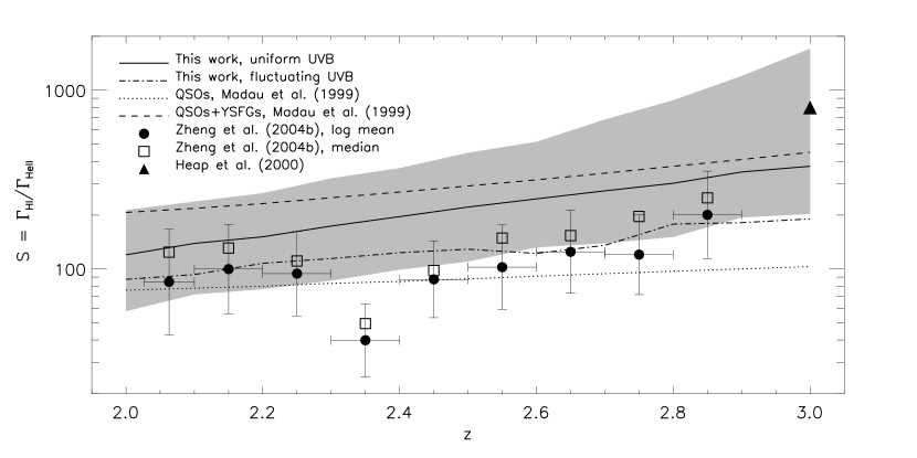
Figure 7: Our determination of the average softness parameter of the UVB compared to the model of MHR99 and other observational estimates. The solid curve shows our results $S$ corrected for resolution effects assuming a spatially uniform UVB. The grey shaded area indicates the theoretical uncertainty. The dot-dashed curves shows our result for the case of a spatially fluctuating He $\rm\scriptstyle II\$ionization rate. The dotted and dashed curves represent the value of $S$ predicted by the updated UVB models of MHR99, based respectively on contributions from QSOs alone and QSOs plus YSFGs. The filled circles with error bars show the results of Z04b calculated from the logarithmic mean of the measured column density ratios $\eta$ using equation 14. The open squares show the median value of $S$ in each redshift bin for the same data. Finally, the filled triangle represents the determination of $S$ at $z\simeq 3$ by Heap et al. (2000).

Our results for the spatially uniform UVB model agree very well with the softness parameter of the updated MHR99 model with contributions from QSOs and YSFGs. At the lowest redshift $z\sim 2$ there is some indication that the MHR99 model may slightly overpredict the softness parameter. Note that the MHR99 UVB model also assumes a spatially uniform background, allowing a fair comparison. Our analysis thus adds to the growing evidence that the amplitude of the UVB at the H $\rm\scriptstyle I\$photoelectric edge cannot be accounted for by QSO emissivities alone; a substantial contribution from YSFGs seems to be required (e.g. Giroux & Shull 1997; Zhang et al. 1997; Theuns et al. 1998; Bianchi et al. 2001; Kriss et al. 2001; Haehnelt et al. 2001; Smette et al. 2002; Zheng et al. 2004b; Shull et al. 2004; Aguirre et al. 2004; Bolton et al. 2005; Kirkman et al. 2005). Note, however, that as discussed before, UV fluctuations will play a significant role in altering $S$ on local scales, especially at $z>2.8$. Some regions of low opacity are obviously subject to a harder ionizing radiation field, producing values of $S$ outside our error range. Similarly, overdense regions which are optically thick to He $\rm\scriptstyle II\$ionizing photons can be subject to a softer radiation field.

The spatial fluctuations also affect the average He $\rm\scriptstyle II\$ionization rate and thus the inferred average softness parameter. The dot-dashed curve in figure 7 shows the average softness parameter obtained from our model of a spatially fluctuating UVB due to QSO emission. The average softness parameter inferred for the spatially fluctuating He $\rm\scriptstyle II\$ionization rate is systematically smaller ($0.15$ dex) than that obtained for a spatially uniform UVB. This is because in regions close to QSOs, corresponding to voids in the He $\rm\scriptstyle II\$Ly$\alpha$ forest, raising the He $\rm\scriptstyle II\$ionization rate further will not decrease the effective optical depth to a great extent once the local optical depth is already low. The average He $\rm\scriptstyle II\$ionization rate will thus be biased low if a uniform background is assumed. This effect is also found for UVB fluctuations at the hydrogen ionization edge (e.g. Gnedin & Hamilton 2002; Meiksin & White 2004).

We also plot the data of Z04b and Heap et al. (2000) in figure 7. The logarithmic mean of the softness parameter calculated from the Z04b column density measurements is shown by the filled circles with error bars. The median value in each bin is indicated with an open square. We have only used data where both the H $\rm\scriptstyle I\$and He $\rm\scriptstyle II\$components have measured column densities; the analysis of our artificial spectra using Voigt profile fitting indicates that these measurements should recover the UVB spectral shape well for the line-of-sight considered, with the median providing a better estimate of $S$. The results of Z04b agree very well with our analysis for a fluctuating He $\rm\scriptstyle II\$ionization rate. Note that the results of Z04b cannot be compared directly to the predictions of the MHR99 model which assumes a spatially uniform UVB.

7 Conclusions

We have used state-of the art hydrodynamical simulations to obtain improved measurements of the spectral shape of the ionizing UV background from the H $\rm\scriptstyle I\$and He $\rm\scriptstyle II\$Ly$\alpha$ forest and to investigate the origin of the large spatial fluctuations observed in the He $\rm\scriptstyle II\$to H $\rm\scriptstyle I\$column density ratio.

Using artificial absorption spectra we have shown that the softness parameter of the UV background can be accurately inferred from the column density ratio of He $\rm\scriptstyle II\$and H $\rm\scriptstyle I\$absorption lines obtained by applying standard Voigt profile fitting routines. Uncertainties in the identification of corresponding H $\rm\scriptstyle I\$and He $\rm\scriptstyle II\$absorption and errors in the determination of the column densities contribute little to the large fluctuations observed in the He $\rm\scriptstyle II\$and H $\rm\scriptstyle I\$column density ratio, although one should be cautious of extreme values of $\eta$. These fluctuations must be due to genuine spatial variations in the spectral shape of the UVB. A model where the He $\rm\scriptstyle II\$ionization rate fluctuates due to variation in the number, luminosity and spectral shape of a small number of QSOs reproduces the observed spatial variations of the He $\rm\scriptstyle II\$and H $\rm\scriptstyle I\$column density ratio, as well as the observed anti-correlation of the column density ratio with the H $\rm\scriptstyle I\$density. This is in good agreement with previous suggestions that the observed He $\rm\scriptstyle II\$Ly$\alpha$ forest spectra at $z\sim 2-3.5$ probes the tail end of the reionization of He $\rm\scriptstyle II\$by QSOs. The large fluctuations observed in the He $\rm\scriptstyle II\$and H $\rm\scriptstyle I\$column density ratio argue strongly against a significant contribution of emission by hot gas to the He $\rm\scriptstyle II\$ionization rate at $2<z<3$.

We further obtain new constraints and error estimates for the mean softness parameter of the UVB and its evolution using the observed effective optical depth of the He $\rm\scriptstyle II\$and H $\rm\scriptstyle I\$Ly$\alpha$ forest. We find that the inferred softness parameter is consistent with a UVB with contributions from QSOs and YSFGs within our uncertainties. The dominant contribution to the uncertainty on $S$ comes from the He $\rm\scriptstyle II\$effective optical depth. Our results for the mean softness parameter add to the growing body of evidence suggesting that a UVB dominated by emission from QSOs alone cannot reproduce the observed effective optical depth of the Ly$\alpha$ forest in QSO spectra.

References

- Abel et al. (1997) Abel T., Anninos P., Zhang Y., Norman M. L., 1997, NewA, 2, 181
- Abel & Haehnelt (1999) Abel T., Haehnelt M. G., 1999, ApJ, 520, L13
- Aguirre et al. (2004) Aguirre A., Schaye J., Kim T., Theuns T., Rauch M., Sargent W. L. W., 2004, ApJ, 602, 38
- Anderson et al. (1999) Anderson S. F., Hogan C. J., Williams B. F., Carswell R. F., 1999, AJ, 117, 56
- Anninos et al. (1997) Anninos P., Zhang Y., Abel T., Norman M. L., 1997, NewA, 2, 209
- Bernardi et al. (2003) Bernardi M., et al. 2003, AJ, 125, 32
- Bi & Davidsen (1997) Bi H., Davidsen A. F., 1997, ApJ, 479, 523
- Bi et al. (1992) Bi H. G., Boerner G., Chu Y., 1992, A&A, 266, 1
- Bianchi et al. (2001) Bianchi S., Cristiani S., Kim T.-S., 2001, A&A, 376, 1
- Bolton et al. (2004) Bolton J., Meiksin A., White M., 2004, MNRAS, 348, L43
- Bolton et al. (2005) Bolton J. S., Haehnelt M. G., Viel M., Springel V., 2005, MNRAS, 357, 1178
- Boyle et al. (2000) Boyle B. J., Shanks T., Croom S. M., Smith R. J., Miller L., Loaring N., Heymans C., 2000, MNRAS, 317, 1014
- Cen (1992) Cen R., 1992, ApJS, 78, 341
- Croft (2004) Croft R. A. C., 2004, ApJ, 610, 642
- Croft et al. (1997) Croft R. A. C., Weinberg D. H., Katz N., Hernquist L., 1997, ApJ, 488, 532
- Croft et al. (1999) Croft R. A. C., Weinberg D. H., Pettini M., Hernquist L., Katz N., 1999, ApJ, 520, 1
- Croom et al. (2004) Croom S. M., Smith R. J., Boyle B. J., Shanks T., Miller L., Outram P. J., Loaring N. S., 2004, MNRAS, 349, 1397
- Davidsen et al. (1996) Davidsen A. F., Kriss G. A., Wei Z., 1996, Nature, 380, 47
- Fardal et al. (1998) Fardal M. A., Giroux M. L., Shull J. M., 1998, AJ, 115, 2206
- Fechner & Reimers (2004) Fechner C., Reimers D., 2004, preprint (astro-ph/0410622)
- Ferrarese & Merritt (2000) Ferrarese L., Merritt D., 2000, ApJ, 539, L9
- Giroux & Shull (1997) Giroux M. L., Shull J. M., 1997, AJ, 113, 1505
- Gleser et al. (2005) Gleser L., Nusser A., Benson A. J., Ohno H., Sugiyama N., 2005, MNRAS, 361, 1399
- Gnedin & Hamilton (2002) Gnedin N. Y., Hamilton A. J. S., 2002, MNRAS, 334, 107
- Haardt & Madau (1996) Haardt F., Madau P., 1996, ApJ, 461, 20
- Haehnelt et al. (2001) Haehnelt M. G., Madau P., Kudritzki R., Haardt F., 2001, ApJ, 549, L151
- Heap et al. (2000) Heap S. R., Williger G. M., Smette A., Hubeny I., Sahu M. S., Jenkins E. B., Tripp T. M., Winkler J. N., 2000, ApJ, 534, 69
- Hernquist et al. (1996) Hernquist L., Katz N., Weinberg D. H., Miralda-Escudé J., 1996, ApJ, 457, L51
- Hogan et al. (1997) Hogan C. J., Anderson S. F., Rugers M. H., 1997, AJ, 113, 1495
- Hui & Gnedin (1997) Hui L., Gnedin N. Y., 1997, MNRAS, 292, 27
- Jakobsen (1996) Jakobsen P., 1996, in Benvenuti P., Macchetto F.D., Schreier E.J., eds, Science with the Hubble Space Telescope - II. Space Telescope Science Institute, Baltimore, p.153
- Jakobsen et al. (1994) Jakobsen P., Boksenberg A., Deharveng J. M., Greenfield P., Jedrzejewski R., Paresce F., 1994, Nature, 370, 35
- Jakobsen et al. (2003) Jakobsen P., Jansen R. A., Wagner S., Reimers D., 2003, A&A, 397, 891
- Katz et al. (1996) Katz N., Weinberg D. H., Hernquist L., 1996, ApJS, 105, 19
- Kirkman et al. (2005) Kirkman D., et al. 2005, MNRAS, 360, 1373
- Kriss et al. (2001) Kriss G. A., et al. 2001, Science, 293, 1112
- Madau et al. (1999) Madau P., Haardt F., Rees M. J., 1999, ApJ, 514, 648
- Madau & Meiksin (1994) Madau P., Meiksin A., 1994, ApJ, 433, L53
- Maselli & Ferrara (2005) Maselli A., Ferrara A., 2005, preprint (astro-ph/0510258)
- McDonald & Miralda-Escudé (2001) McDonald P., Miralda-Escudé J., 2001, ApJ, 549, L11
- McDonald et al. (2001) McDonald P., Miralda-Escudé J., Rauch M., Sargent W. L. W., Barlow T. A., Cen R., 2001, ApJ, 562, 52
- Meiksin & White (2004) Meiksin A., White M., 2004, MNRAS, 350, 1107
- Miniati et al. (2004) Miniati F., Ferrara A., White S. D. M., Bianchi S., 2004, MNRAS, 348, 964 (M04)
- Miralda-Escudé (1993) Miralda-Escudé J., 1993, MNRAS, 262, 273
- Miralda-Escudé et al. (1996) Miralda-Escudé J., Cen R., Ostriker J. P., Rauch M., 1996, ApJ, 471, 582
- Miralda-Escudé et al. (2000) Miralda-Escudé J., Haehnelt M., Rees M. J., 2000, ApJ, 530, 1
- Miralda-Escudé & Ostriker (1990) Miralda-Escudé J., Ostriker J. P., 1990, ApJ, 350, 1
- Rauch (1998) Rauch M., 1998, ARA&A, 36, 267
- Rauch et al. (1997) Rauch M., et al. 1997, ApJ, 489, 7
- Reimers et al. (2005a) Reimers D., Fechner C., Hagen H.-J., Jakobsen P., Tytler D., Kirkman D., 2005a, A&A, 442, 63
- Reimers et al. (2004) Reimers D., Fechner C., Kriss G., Shull M., Baade R., Moos W., Songaila A., Simcoe R., 2004, preprint (astro-ph/0410588)
- Reimers et al. (2005b) Reimers D., Hagen H.-J., Schramm J., Kriss G. A., Shull J. M., 2005b, A&A, 436, 465
- Reimers et al. (1997) Reimers D., Kohler S., Wisotzki L., Groote D., Rodriguez-Pascual P., Wamsteker W., 1997, A&A, 327, 890
- Richards et al. (2005) Richards G. T., et al. 2005, MNRAS, 360, 839
- Ricotti et al. (2000) Ricotti M., Gnedin N. Y., Shull J. M., 2000, ApJ, 534, 41
- Schaye et al. (2003) Schaye J., Aguirre A., Kim T., Theuns T., Rauch M., Sargent W. L. W., 2003, ApJ, 596, 768
- Schaye et al. (2000) Schaye J., Theuns T., Rauch M., Efstathiou G., Sargent W. L. W., 2000, MNRAS, 318, 817
- Scott et al. (2004) Scott J. E., Kriss G. A., Brotherton M., Green R. F., Hutchings J., Shull J. M., Zheng W., 2004, ApJ, 615, 135
- Shull et al. (2004) Shull J. M., Tumlinson J., Giroux M. L., Kriss G. A., Reimers D., 2004, ApJ, 600, 570
- Smette et al. (2002) Smette A., Heap S. R., Williger G. M., Tripp T. M., Jenkins E. B., Songaila A., 2002, ApJ, 564, 542
- Sokasian et al. (2002) Sokasian A., Abel T., Hernquist L., 2002, MNRAS, 332, 601
- Songaila (1998) Songaila A., 1998, AJ, 115, 2184
- Spergel et al. (2003) Spergel D. N., et al. 2003, ApJS, 148, 175
- Springel (2005) Springel V., 2005, preprint (astro-ph/0505010)
- Springel et al. (2001) Springel V., Yoshida N., White S. D. M., 2001, NewA, 6, 79
- Storrie-Lombardi et al. (1994) Storrie-Lombardi L. J., McMahon R. G., Irwin M. J., Hazard C., 1994, ApJ, 427, L13
- Telfer et al. (2002) Telfer R. C., Zheng W., Kriss G. A., Davidsen A. F., 2002, ApJ, 565, 773
- Theuns et al. (1998) Theuns T., Leonard A., Efstathiou G., Pearce F. R., Thomas P. A., 1998, MNRAS, 301, 478
- Theuns et al. (2002) Theuns T., Schaye J., Zaroubi S., Kim T., Tzanavaris P., Carswell B., 2002, ApJ, 567, L103
- Tytler et al. (1995) Tytler D., Fan X.-M., Burles S., Cottrell L., Davis C., Kirkman D., Zuo L., 1995, in Meylan G., ed, Proc. of ESO Workshop, QSO Absorption Lines. Springer-Verlag, Berlin, p.289
- Wadsley et al. (1999) Wadsley J. W., Hogan C. J., Anderson S. F., 1999, in Holt S., Smith E., eds, AIP Conf. Proc. 470: After the Dark Ages: When Galaxies were Young (the Universe at 2 z 5). American Institute of Physics Press, p.273
- Walker et al. (1991) Walker T. P., Steigman G., Kang H., Schramm D. M., Olive K. A., 1991, ApJ, 376, 51
- Weinberg et al. (1998) Weinberg D. H., Hernquist L., Katz N., Croft R., Miralda-Escudé J., 1998, in Petitjean P., Charlot S., eds, Proc. 13th IAP Colloq., Structure and Evolution in the Intergalactic Medium. Editions Frontiéres, Paris, p.133
- Zhang et al. (1997) Zhang Y., Anninos P., Norman M. L., Meiksin A., 1997, ApJ, 485, 496
- Zhang et al. (1998) Zhang Y., Meiksin A., Anninos P., Norman M. L., 1998, ApJ, 495, 63
- Zheng et al. (2004a) Zheng W., Chiu K., Anderson S. F., Schneider D. P., Hogan C. J., York D. G., Burles S., Brinkmann J., 2004a, AJ, 127, 656
- Zheng & Davidsen (1995) Zheng W., Davidsen A., 1995, ApJ, 440, L53
- Zheng et al. (1998) Zheng W., Davidsen A. F., Kriss G. A., 1998, AJ, 115, 391
- Zheng et al. (2004b) Zheng W., et al. 2004b, ApJ, 605, 631 (Z04b)