Imaging redshifts of BL Lac objects.

Abstract

The HST snapshot imaging survey of 110 BL Lac objects (Urry et al., 2000) has clearly shown that the host galaxies are massive and luminous ellipticals. The dispersion of the absolute magnitudes is sufficiently small, so that the measurement of the galaxy brightness becomes a valuable way of estimating their distance. This is illustrated constructing the Hubble diagram of the 64 resolved objects with known redshift. By means of this relationship we estimate the redshift of five resolved BL Lacs of the survey, which have no spectroscopic $z$. The adopted method allows us also to evaluate lower limits to the redshift for 13 objects of still unknown $z$, based on the lower limit on the host galaxy magnitude. This technique can be applied to any BL Lac object for which an estimate or a lower limit of the host galaxy magnitude is available. Finally we show that the distribution of the nuclear luminosity of all the BL Lacs of the survey, indicates that the objects for which both the redshift and the host galaxy are undetected, are among the most luminous, and possibly the most highly beamed.

1 Introduction

Contrary to the large majority of Active Galactic Nuclei (AGN), characterized by optical spectra with prominent emission lines, BL Lac objects have quasi featureless spectra. In fact by the definition of this class of AGN, the line equivalent widths should be very small. The effect of this weakness of the spectral features has the consequence to hamper in many cases the determination of the redshift, thus making the distance of the source difficult to assess. As originally proposed by Blandford & Rees (1978), the weakness of the spectral lines is most probably due to the fact that the underlying non thermal continuum is exalted by the relativistic beaming of a jet pointing in the observer direction.

There are two possible strategies for deriving the distance (redshift) of BL Lacs. The first one is to improve the S/N ratio of the optical spectra, so that very weak spectral features may become detectable. At present some significant progress with respect to the existing data can be obtained through the use of 8m class telescopes (e.g. Heidt et al., 2004; Sbarufatti et al., 2005a, b; Sowards-Emmerd et al., 2005).

The second approach requires high quality imaging of the objects, with the scope of detecting the host galaxy. Using it as a standard candle one can obtain an albeit indirect estimate of the distance (e.g. Romanishin, 1987; Falomo, 1996; Falomo & Kotilainen, 1999; Heidt et al., 1999; Nilsson et al., 2003). For this approach one needs a combination of superb angular resolution and high efficiency, in order to detect and characterize the faint extended light of the galaxy from the bright nucleus. These conditions become mandatory at high redshifts, because of the dimming of the surface brightness, which scales as (1+z)⁴.

The first imaging studies of BL Lac hosts were carried out using ground based telescopes which produced a preliminary characterization of the properties of host galaxies for various datasets (e.g. Abraham et al., 1991; Falomo, 1996; Wurtz et al., 1996; Falomo & Kotilainen, 1999; Heidt et al., 1999; Nilsson et al., 2003). These works have consistently shown that BL Lac hosts are virtually all massive ellipticals (average luminosity M_R =–23.7 and effective radius R${}_{e}\sim$ 10 kpc, assuming H₀=50 km s^-1 Mpc^-1, $\Omega$=0). A substantial progress in this area was achieved through the use of HST images, and in particular by the BL Lac snapshot survey, carried out with WFPC2. This produced high quality homogeneous images for 110 objects (Falomo et al., 1997; Urry et al., 1999; Scarpa et al., 2000a, b; Urry et al., 2000; Falomo et al., 2000; O’Dowd & Urry, 2005).

In this paper we reconsider the results of the HST snapshot survey, with the aim of fully exploiting the information relevant for the determination of the distance of BL Lacs. The starting point is the analysis of the absolute magnitude distribution of the hosts. We show that since this distribution is relatively narrow one can indeed use the host luminosity as a standard candle to evaluate the redshift. This is used in particular to determine the redshift for objects the host galaxy of which is detected, but that still have featureless spectra. We then focus on the nuclei of the sources, and show that the unresolved objects with pure featureless spectra are likely the most luminous and possibly beamed objects of the class.

2 HST Images of BL Lacs

For this work we have considered the dataset of images obtained by the HST BL Lac survey discussed by Urry et al. (2000, in the following addressed as U00). It contains 110 objects imaged with HST+WFPC2 in the F702W filter. The U00 sample was selectted from seven flux limited BL Lac samples in literature (1Jy, PG, HEAO-A2, HEAO-A3, EMSS, Slew). It includes both high energy peaked (HBL) and low energy peaked (LBL) objects (see Padovani & Giommi, 1995, for HBL and LBL definition), covering a wide range of jet physics in BL Lacs. The surface brightness profile for each object was modeled with a combination of a point source (the nucleus component), and an extended emission (the host galaxy) represented by an elliptical (de Vaucouleurs law) or a disk component (exponential law). For all the sources where the host galaxy can be detected the radial brightness profile is consistent with the host being an elliptical. For the unresolved sources, U00 give a lower limit on the apparent magnitude of the underlying nebulosity.

In order to construct a more homogeneous and updated dataset of BL Lac host galaxies measurements we have introduced a number of revisions in the treatment of the results of U00, which are listed in the following:

1. For three objects 0145+138, 0446+449, 0525+713 there is no evidence of a nuclear component in the HST images. This makes the classification as BL Lac dubious, and therefore they are not considered here. The object 1320+084 has been excluded from the sample, since recent spectroscopy (Sbarufatti et al., 2005b) has shown that the source is a broad line QSO at z=1.5. Our sample is then reduced to 106 objects;

2. For four objects new redshifts have been published in the last years: 0426-380, 1519-273 (Sbarufatti et al., 2005a), 0754+100; 1914-194 (Carangelo et al., 2003), and for one ( 0158+001) the redshift was revised (SDSS);

3. The galactic extinction is now accounted for following Schlegel, Finkbeiner, & Davis (1998);

4. The K-correction for galaxy magnitudes is taken from Poggianti (1997);

5. The adopted cosmological parameters are: H₀= 70 km s^-1 Mpc^-1, $\Omega_{\Lambda}$=0.7, $\Omega_{m}$=0.3;

6. In order to compare the luminosity of the hosts at different redshifts (and epochs) we have also included a correction for taking into account the passive evolution of the galaxies following Bressan et al. (1998) prescriptions. This correction, weighted on the redshift distribution, is $\sim$0.3 magnitudes.

Table 1 reports the relevant parameters for the 106 objects. According to the spectra and imaging properties the objects in the sample can be divided in 4 groups:

• Objects for which the redshift is known from spectroscopy, and the host galaxy is detected (N= 64). All the sources with z$\leq$0.2 belong to this class (see Falomo et al., 2000);

• Objects for which the host galaxy has been detected but with unknown redshift (N= 5);

• Objects of known redshift but for which the host galaxy has not been detected (N=24);

• Objects of unknown redshift and that have not been resolved by HST optical imaging (N= 13).

The redshift distribution of these groups is given in Fig. 1. As expected the objects in group A are clustered at low redshift (z $<$ 0.5) while those that are unresolved tend to be at z $>$ 0.5.

3 Results

3.1 The Hubble diagram of the host galaxies of BL Lacs

The absolute magnitude of each host galaxy, modified for the effects of K and evolution correction (Poggianti, 1997; Bressan et al., 1998) is reported in Table 1. The distribution of the absolute magnitude (M_R) of the host galaxies for objects in group A is reported in Fig. 2. This distribution is rather narrow and can be well approximated by a Gaussian with mean value $<$M${}_{R}>$=–22.8 and standard deviation $\sigma_{M}$=0.5. Note that U00 reported $<$M${}_{R}>$=–23.7$\pm$0.6. The main difference is due to the difference in cosmological parameters (U00 used H₀= 50 km s^-1 Mpc^-1, $\Omega$=0) and to the addition of the correction for the passive evolution of the galaxies. These variations also produce a smaller dispersion of the distribution (0.5 with respect to 0.6 given in U00).

In order to test how the host galaxy luminosity of BL Lacs can be used as a standard candle we have constructed the Hubble diagram. The relation between the apparent magnitude m_R of the host galaxy and the redshift $z$ is given by:

$$\textrm{m}_{R}=\textrm{M}_{R}-\textrm{K}(z)+\textrm{E}(z)-5+5\textrm{log}(\textrm{d}(z))$$ (1)

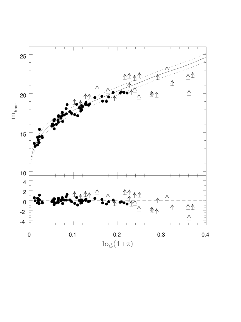
Figure 3: Hubble diagram for host galaxies of BL Lacs. Apparent magnitudes (R filter) are corrected for the galactic extinction. Group A (host detected, redshift known): filled circles. Group C (host undetected, redshift known) objects are shown as upper limits. The solid line corresponds to a fit with a galaxy of M_R=M${}_{R}^{fit}$=–22.9. Dotted curves correspond to a host galaxy 0.5 magnitudes brighter (lower curve) or fainter (upper curve). Lower panel shows the deviations of the data from the fit.

where M_R is the host absolute magnitude, K($z$) is the K-correction, E($z$) is the evolution correction, d($z$) is the luminosity distance. With the assumptions described above for the cosmology and the K and passive evolution corrections, the only remaining free parameter is the host magnitude M_R. The best fit of the observed data yields M${}_{R}^{fit}$=–22.9. The Hubble diagram (m_R vs. $z$) for the BL Lac hosts together with the best fit is shown in Fig. 3. It is noticeable that $\sim$ 70% of the points representing the resolved BL Lacs are encompassed within M${}_{R}^{fit}$$\pm$0.5 mag (i.e. –23.4$<$M${}_{R}<$–22.4). This Hubble diagram can be used to obtain a photometric redshift of the objects from the measurement of the host galaxy apparent magnitude, or a lower limit on $z$ if only a lower limit on the magnitude is available. In the redshift range considered here ($z\lesssim$0.7) the Hubble diagram can be well represented by the following expression:

$$\textrm{log}(1+z)=\ (0.293*\textrm{m}_{R}^{2}+7.19*\textrm{m}_{R}+45.1)*10^{-2},$$ (2)

which approximates the Hubble diagram with a precision better than 1%.

To evaluate the capability of this method we compare in Fig. 4 the redshifts given by this photometric technique with the redshifts derived from the spectra in all cases where it is available. The comparison shows that, apart very few exceptions, the $z$ estimated by the host galaxy luminosity is in very good agreement with the one obtained spectroscopically. The average difference of redshift between the two methods is:

$$<\Delta z>=0.01\pm 0.05(rms).$$ (3)

The main conclusion of this analysis is therefore that, at least in the explored redshift range ($z<$ 0.7), the measurement of the apparent magnitude of the host galaxy of a BL Lac source allows one to estimate its redshift with an average accuracy of 0.05. Because the U00 sample is unbiased as far as host galaxies are concerned, this technique can be of use any time that the R apparent magnitude of a BL Lac host galaxy is measured, or a lower limit is obtained. In particular, equation 2 gives a straightforward method to estimate the redshift in such cases. In the following sections we will use this technique to derive the redshift or a lower limit for the objects in groups B, C, and D.

3.2 Imaging redshifts

Group B (host galaxy detected, unknown spectroscopic redshift)

Using the fit derived above for the Hubble diagram we can get a photometric estimate of the redshift for the 5 objects with host detected and no spectroscopic $z$ available (see Table 1; group B). The redshift of these objects ranges from $z$ = 0.26 to $z$ =0.54. Combining the uncertainty deriving from equation (3) with the one corresponding to the host galaxy apparent magnitude (which is of the order of 0.1 mag), the error on the imaging redshifts turns out to be $\lesssim$0.1. From the estimated $z$, one can then obtain the nucleus luminosity. For the nucleus we adopted a K-correction following Wisotzki (2000), under the hypothesis that its optical spectrum is described by a power law (F${}_{\lambda}\propto\lambda^{-\alpha}$ with $\alpha$=0.7, see Falomo et al., 1994). Results are reported in Table 1.

Group C (redshift known, host undetected)

From the HST images of these sources we have a lower limit on the magnitude of the host reported by U00 (see Table 1) and we know the redshift from the spectra. From these values we can obtain a lower limit on the absolute magnitude of the host galaxy. These limits are in most cases consistent (see Fig. 3) with the presence of a host galaxy less luminous than M_R=–23.4 (i.e. M${}_{R}^{fit}$–0.5). In no case the derived limit for the host luminosity is lower than M_R=–21.9 (i.e. M${}_{R}^{fit}$+1.0). Therefore the fact that the host galaxy has not been detected in these HST images is consistent with the capability of the observation and with a distribution of the host absolute magnitude as given in Fig. 2. The non detection of the host in most cases is likely due to a high nuclear to host galaxy ratio (see section 4 and Fig. 6).

Group D (no host, no redshift: extreme BL Lacs)

The remaining group of objects is that formed by the unresolved sources which exhibit a featureless spectrum. The redshift of these objects is thus far still unknown. The only information that can be derived from the images is therefore the brightness of the nucleus and an upper limit to the brightness of the surrounding nebulosity. Assuming that also these objects are hosted in a galaxy with M_R=M${}_{R}^{fit}$=–22.9 and from the lower limit of the magnitude of the surrounding nebulosity one can derive a lower limit to the redshift using the Hubble diagram (see Fig. 3 and Table 1). This lower limit to the redshift can then be used to derive a lower limit to the luminosity of the nucleus. The distribution of the absolute magnitude of the nuclei for all objects in the four groups is shown in Fig 5. It turns out that most of the sources in group D are more luminous than M_R=–25 and fill the bright tail of the luminosity distribution. It is worth to note also that of the 13 objects in this group, 10 are HBL and only 3 are LBL, while in the whole sample there are 71 HBL and 35 LBL.

4 Discussion: nuclear luminosities and beaming.

We have shown that the detection of the host galaxy allows a photometric determination of the redshift for the 5 objects in group B. Since these objects are at 0.2$<z<$0.5 they are convenient targets for redshift measurement through spectroscopy. Direct estimates of the absolute nuclear magnitude are available for the objects with known spectroscopic redshift (group A and C). In addition, using the imaging redshifts we can add 5 more targets (group B objects) and 13 upper limits for the objects in group D. The redshift distribution of the whole sample is given in Fig. 1.

The absolute nuclear magnitudes are summarized in Table 1. The mean and median absolute magnitude for objects in the groups A+B+C are M_R=–23.7 and M_R=–23.6 respectively, while adding objects in group D the median is M_R=–24.1. As already noted by U00 the distribution of the absolute magnitude of the host galaxies is much narrower than that of their nuclei (Fig. 5).

Since the objects in each individual sample used to produce the HST snapshot survey are selected on the basis of their radio and X-ray fluxes, it is expected that the entire dataset of objects suffers from the typical bias of the flux limited surveys. Nevertheless some interesting comments should be made. Our analysis of the redshift and the nuclear luminosity of the objects clearly shows that the extreme BL Lacs (objects with featureless spectra and unresolved; group D), are among the most luminous sources in the sample. Indeed 10 out of 13 objects are brighter than the brightest object in the group A (see Fig. 5a). If one compares the luminosity distribution with that of z $<$ 1.4 radio loud quasars (using homogeneous corrections for the magnitudes) used for the BL Lacs it is apparent that the bright tail of the BL Lacs distribution is consistent with that of normal radio loud quasars (see Fig 5b).

Below the absolute magnitude M_R=–25 there are basically two types of objects (groups C and D). Unless the latter are really significantly more luminous than the average of objects in group C (objects with emission lines) the different spectral properties could be related to different amount of beaming. If one assumes that the two types of objects have a similar Broad Line Region, the strength of the line should be related to the intrinsic ionizing flux. If blazars behave as normal quasars the line emission should depend on the unbeamed continuum (e.g. Pian et al., 2005, and references therein). Under this hypothesis therefore we argue that in extreme BL Lacs the mechanism for emission line formation is less efficient because the intrinsic continuum source is smaller with respect to group C objects, but more strongly beamed.

This suggestion is made stronger by the consideration of the distribution of the objects in the plane m_R vs. $z$ (see Fig. 6). The curves represent the loci of a constant Nucleus/Host ratio (N/H), defined as the ratio of monochromatic R band luminosities in the object rest frame. All the resolved sources are in the region with N/H less than 10 while the large majority of objects in groups C and D are in the region between N/H=10 and N/H = 1000. Again in this context group D objects are clearly the most extreme, implying high N/H ratios (sometimes in excess of N/H=100). It is also noticeable that group D objects are mostly of the HBL type , while the majority of group C objects are of the LBL type. The inference is therefore that in the optical band HBLs are more beamed than LBLs.

Independent information on the amount of beaming can be derived from the broad band spectral energy distribution, assuming that the emitted continuum is basically the superposition of a synchrotron and an inverse Compton component (see e.g. Ghisellini et al., 1998). Thus far these studies were limited to objects of known redshifts, which is irrelevant to our proposal that extreme BL Lacs are extremely beamed objects, but some extension to this class of sources may soon become available.

5 Conclusions

We have reanalyzed the host galaxies and nuclear properties of the BL Lac objects observed by HST snapshot imaging survey. The magnitudes of the objects in the dataset have been revised according to the treatment of the galactic extinction, the evolution and K-corrections. The concordant cosmological parameters have been used.

The main results and conclusions from this study are:

• The host galaxy absolute magnitude distribution is sufficiently narrow (gaussian distribution centered around M_R=–22.9) that the host galaxy can be used as a standard candle to derive the photometric redshift of the objects. Therefore a determination of $z$ (or a lower limit) can be simply derived from the measurement (or from the lower limit) of the host galaxy apparent magnitude.

• The determination of the redshift and the lower limits allow us to investigate the nuclear luminosity distributions for various type of objects. This suggests that the objects in the sample that are unresolved and characterized by a featureless spectrum are the most luminous and /or beamed nuclei of the class. These extreme BL Lacs could have a nucleus-to-host galaxy ratio of 100 to 1000.

Figure 1: Redshift distribution of BL Lac objects in the HST snapshot imaging survey. Group A (host detected, redshift known): shaded. Group B (host detected, redshift unknown): slashed. Group C (host undetected, redshift known): open+ arrow. Group D (host undetected, redshift unknown): open. Lower limits are represented by arrows.

Figure 2: The distribution of the host galaxy absolute magnitude M_R for objects of group A (host galaxy detected; redshift known). The solid line represents a gaussian fit to the distribution (mean M_R=–22.8, $\sigma$=0.5).

Figure 4: Comparison between imaging redshift obtained using the Hubble diagram fit and the spectroscopic redshift for the objects in group A (host detected, redshift known). The solid line represent the one to one relation.

Figure 5: Upper panel (a): Distribution of nucleus absolute magnitude of BL Lacs in the R filter. Group A+B (host detected): cross-hatched. Group C (host undetected, redshift known): slashed. Group D (host undetected, redshift unknown): open+arrow. The solid line represents the gaussian fit to the host galaxy absolute magnitude distribution for group A, scaled by a factor 0.5. Upper limits are represented by arrows. Lower panel (b): Distribution of absolute R magnitudes for radio loud quasars (RL QSO) in Véron-Cetty & Véron (2003) catalogue with $z<$1.4.

Figure 6: Distribution of nucleus apparent magnitude (corrected for galactic extinction) vs. redshift. Dashed lines show the loci of constant nucleus-to-host ratio (N/H), assuming a host galaxy with M_R=M${}_{R}^{fit}$=–22.9. Group A (host detected, redshift known): filled circles. Group B (host detected, redshift unknown): open circles (redshift estimated using Hubble diagram. Group C (host undetected, redshift known): open triangles. Group D (host undetected, redshift unknown): arrows (lower limits on redshift determined using Hubble diagram).

Table 1: Host galaxy and nuclear properties of BL Lac objects

object	type	group	AR	z	Galaxy	Nucleus	Evolution	mn	Mn	mh	Mh
					K corr.	K corr.	corr.
(1)	(2)	(3)	(4)	(5)	(6)	(7)	(8)	(9)	(10)	(11)	(12)
0033+595	H	D	2.354	[$>$0.24]	0.71	0.06	$-$0.39	18.23	$<$$-$24.25	$>$20.00	$-$22.90
0118$-$272	L	C	0.036	0.559	0.91	0.14	$-$0.43	15.78	$-$26.96	$>$19.09	$>$$-$23.86
0122+090	H	A	0.249	0.339	0.43	0.10	$-$0.28	21.98	$-$19.65	18.88	$-$22.67
0138$-$097	L	C	0.079	0.733	1.4	0.18	$-$0.61	17.68	$-$25.87	$>$20.19	$>$$-$23.84
0158+001	H	A	0.064	0.298	0.36	0.08	$-$0.24	18.38	$-$22.72	18.27	$-$22.75
0229+200	H	A	0.360	0.139	0.15	0.04	$-$0.14	18.58	$-$20.93	15.85	$-$23.54
0235+164	L	C	0.211	0.940	2.01	0.22	$-$0.78	18.18	$-$26.21	$>$19.75	$>$$-$25.55
0257+342	H	A	0.468	0.247	0.29	0.07	$-$0.21	19.18	$-$21.86	17.93	$-$22.99
0317+183	H	A	0.369	0.190	0.21	0.06	$-$0.17	18.28	$-$22.09	17.59	$-$22.57
0331$-$362	H	A	0.050	0.308	0.38	0.09	$-$0.25	19.03	$-$22.15	17.81	$-$23.28
0347$-$121	H	A	0.125	0.188	0.21	0.06	$-$0.17	18.28	$-$21.74	17.72	$-$22.17
0350$-$371	H	A	0.020	0.165	0.18	0.05	$-$0.16	18.03	$-$21.60	17.08	$-$22.38
0414+009	H	A	0.314	0.287	0.35	0.08	$-$0.24	16.08	$-$25.19	17.49	$-$23.67
0419+194	H	A	1.476	0.512	0.79	0.13	$-$0.40	19.53	$-$24.44	21.05	$-$23.02
0426$-$380	L	C	0.066	1.105	2.44	0.24	$-$0.94	18.08	$-$26.61	$>$21.10	$>$$-$24.80
0454+844	L	C	0.316	1.340	3.04	0.28	$-$1.11	18.20	$-$27.30	$>$22.37	$>$$-$24.79
0502+675	H	A	0.406	0.314	0.39	0.09	$-$0.26	17.33	$-$24.28	18.86	$-$22.64
0506$-$039	H	A	0.220	0.304	0.37	0.09	$-$0.25	18.73	$-$22.61	18.35	$-$22.87
0521$-$365	L	A	0.105	0.055	0.06	0.02	$-$0.06	15.28	$-$21.99	14.60	$-$22.43
0537$-$441	L	C	0.101	0.896	1.89	0.21	$-$0.74	15.83	$-$28.30	$>$19.66	$>$$-$25.32
0548$-$322	H	A	0.094	0.069	0.07	0.02	$-$0.08	16.93	$-$20.68	14.62	$-$22.89
0607+710	H	A	0.512	0.267	0.32	0.08	$-$0.22	18.23	$-$23.06	17.83	$-$23.35
0622$-$525	H	B	0.241	[0.41]	0.54	0.11	$-$0.33	18.83	$-$23.26	19.37	$-$22.90
0647+250	H	D	0.264	[$>$0.47]	0.48	0.11	$-$0.33	15.18	$<$$-$26.93	$>$19.10	$-$22.90
0706+591	H	A	0.103	0.125	0.14	0.04	$-$0.13	17.53	$-$21.54	15.94	$-$22.95
0715$-$259	H	A	0.989	0.465	0.68	0.12	$-$0.37	18.13	$-$25.08	20.02	$-$23.23
0716+714	H	D	0.082	[$>$0.52]	0.71	0.13	$-$0.39	14.18	$<$$-$28.34	$>$20.00	$-$22.90
0735+178	L	C	0.094	0.424	0.59	0.12	$-$0.34	16.58	$-$25.50	$>$20.44	$>$$-$21.62
0737+744	H	A	0.073	0.315	0.39	0.09	$-$0.26	17.88	$-$23.40	18.01	$-$23.16
0749+540	L	C	0.111	0.730	1.39	0.18	$-$0.61	16.23	$-$27.35	$>$21.78	$>$$-$22.26
0754+100	L	C	0.060	0.266	0.32	0.08	$-$0.22	16.03	$-$24.80	$>$18.69	$>$$-$22.03
0806+524	H	A	0.118	0.138	0.15	0.04	$-$0.14	15.98	$-$23.28	16.62	$-$22.51
0814+425	L	D	0.170	[$>$0.75]	1.25	0.19	$-$0.57	18.99	$<$$-$24.90	$>$21.47	$-$22.90
0820+225	L	C	0.112	0.951	2.04	0.22	$-$0.79	19.98	$-$24.34	$>$21.90	$>$$-$23.36
0823+033	L	C	0.122	0.506	0.78	0.13	$-$0.40	17.78	$-$24.79	$>$20.18	$>$$-$22.49
0828+493	L	A	0.117	0.548	0.88	0.14	$-$0.43	18.93	$-$23.84	20.26	$-$22.69
0829+046	L	A	0.087	0.180	0.2	0.05	$-$0.17	15.88	$-$24.08	16.94	$-$22.80
0851+202	L	C	0.076	0.306	0.38	0.09	$-$0.25	14.99	$-$26.21	$>$18.53	$>$$-$22.57
0922+749	H	A	0.091	0.638	1.12	0.16	$-$0.50	20.13	$-$23.04	20.25	$-$23.25
0927+500	H	A	0.045	0.188	0.21	0.06	$-$0.17	17.48	$-$22.46	17.62	$-$22.19
0954+658	L	C	0.306	0.367	0.48	0.10	$-$0.30	16.08	$-$25.81	$>$19.60	$>$$-$22.24
0958+210	H	A	0.061	0.344	0.44	0.10	$-$0.28	21.48	$-$20.02	18.93	$-$22.48
1011+496	H	A	0.033	0.200	0.23	0.06	$-$0.18	15.88	$-$24.28	17.30	$-$22.66
1028+511	H	A	0.033	0.361	0.47	0.10	$-$0.29	16.48	$-$25.13	18.55	$-$22.97
1044+549	H	B	0.038	[0.54]	0.73	0.13	$-$0.39	19.88	$-$22.59	20.05	$-$22.90
1104+384	H	A	0.041	0.031	0.03	0.01	$-$0.03	13.78	$-$22.49	13.29	$-$22.40
1106+244	H	B	0.045	[0.46]	0.59	0.13	$-$0.33	18.28	$-$24.20	19.57	$-$22.90
1133+161	H	A	0.173	0.460	0.67	0.12	$-$0.37	20.28	$-$22.11	19.83	$-$22.57
1136+704	H	A	0.035	0.045	0.05	0.01	$-$0.05	16.15	$-$20.63	14.45	$-$22.06
1144$-$379	L	C	0.257	1.048	2.3	0.23	$-$0.88	17.28	$-$27.44	$>$23.03	$>$$-$22.82
1147+245	H	D	0.073	[$>$0.63]	0.95	0.15	$-$0.46	16.87	$<$$-$26.13	$>$20.70	$-$22.90
1207+394	H	A	0.079	0.615	1.06	0.16	$-$0.48	19.48	$-$23.59	20.30	$-$23.05
1212+078	H	A	0.059	0.136	0.15	0.04	$-$0.14	16.38	$-$22.82	16.02	$-$23.02
1215+303	H	A	0.064	0.130	0.14	0.04	$-$0.13	14.55	$-$24.64	15.99	$-$22.95
1218+304	H	A	0.056	0.182	0.2	0.05	$-$0.17	15.68	$-$24.25	17.12	$-$22.62
1221+245	H	A	0.048	0.218	0.25	0.06	$-$0.19	16.89	$-$23.41	18.63	$-$21.56
1229+643	H	A	0.049	0.164	0.18	0.05	$-$0.16	18.03	$-$21.63	16.38	$-$23.09
1239+069	H	D	0.057	[$>$0.92]	1.63	0.21	$-$0.75	18.45	$<$$-$25.66	$>$22.30	$-$22.90
1246+586	H	D	0.029	[$>$0.73]	1.14	0.17	$-$0.57	15.66	$<$$-$27.72	$>$21.20	$-$22.90
1248$-$296	H	A	0.202	0.370	0.49	0.10	$-$0.30	18.83	$-$23.02	18.87	$-$22.89
1249+174	H	C	0.058	0.644	1.14	0.16	$-$0.51	18.51	$-$24.66	$>$21.90	$>$$-$21.60
1255+244	H	A	0.034	0.141	0.15	0.04	$-$0.14	17.08	$-$22.25	16.72	$-$22.38
1402+041	H	C	0.069	0.340	0.43	0.10	$-$0.28	16.38	$-$25.12	$>$19.38	$>$$-$22.00
1407+595	H	A	0.037	0.495	0.75	0.13	$-$0.39	18.84	$-$23.59	19.04	$-$23.47
1418+546	L	A	0.036	0.152	0.17	0.05	$-$0.15	15.68	$-$23.82	16.10	$-$23.18
1422+580	H	C	0.027	0.683	1.25	0.17	$-$0.55	18.35	$-$24.95	$>$21.99	$>$$-$21.71
1424+240	H	D	0.156	[$>$0.67]	1.06	0.17	$-$0.57	14.66	$<$$-$28.85	$>$21.00	$-$22.90
1426+428	H	A	0.033	0.129	0.14	0.04	$-$0.13	17.38	$-$21.63	16.14	$-$22.75
1437+398	L	B	0.037	[0.26]	0.29	0.09	$-$0.18	16.73	$-$24.43	17.95	$-$22.90
1440+122	H	A	0.076	0.162	0.18	0.05	$-$0.15	16.93	$-$22.75	16.71	$-$22.77
1458+224	H	A	0.128	0.235	0.27	0.07	$-$0.20	15.78	$-$24.82	17.80	$-$22.65
1514$-$241	H	A	0.369	0.049	0.05	0.02	$-$0.05	14.48	$-$22.65	14.45	$-$22.58
1517+656	H	C	0.068	0.702	1.3	0.17	$-$0.58	16.18	$-$27.24	$>$19.89	$>$$-$23.94
1519$-$273	L	C	0.636	1.297	2.92	0.27	$-$1.09	17.03	$-$28.69	$>$20.40	$>$$-$26.88
1533+535	H	C	0.051	0.890	1.87	0.21	$-$0.74	17.88	$-$26.19	$>$19.70	$>$$-$25.19
1534+014	H	A	0.152	0.312	0.39	0.09	$-$0.25	19.08	$-$22.27	18.16	$-$23.08
1538+149	L	A	0.148	0.605	1.03	0.15	$-$0.46	17.94	$-$25.14	20.22	$-$23.14
1544+820	H	D	0.133	[$>$0.46]	0.60	0.13	$-$0.33	16.55	$<$$-$26.02	$>$19.60	$-$22.90
1553+113	H	D	0.139	[$>$0.78]	1.31	0.21	$-$0.68	14.43	$<$$-$29.76	$>$21.60	$-$22.90
1704+604	H	A	0.062	0.280	0.33	0.08	$-$0.23	21.08	$-$19.92	18.69	$-$22.15
1722+119	H	D	0.458	[$>$0.68]	1.23	0.17	$-$0.57	14.61	$<$$-$29.20	$>$21.40	$-$22.90
1728+502	H	A	0.079	0.055	0.06	0.02	$-$0.06	16.43	$-$20.81	15.49	$-$21.51
1738+476	L	D	0.050	[$>$0.60]	0.87	0.15	$-$0.39	19.63	$<$$-$23.35	$>$20.50	$-$22.90
1745+504	H	B	0.086	[0.46]	0.59	0.13	$-$0.33	21.18	$-$21.34	19.57	$-$22.90
1749+096	L	A	0.482	0.320	0.4	0.09	$-$0.26	16.88	$-$24.88	18.82	$-$22.81
1749+701	L	C	0.083	0.770	1.51	0.19	$-$0.65	15.83	$-$27.87	$>$19.28	$>$$-$24.96
1757+703	H	A	0.089	0.407	0.56	0.11	$-$0.33	18.43	$-$23.52	19.58	$-$22.35
1803+784	L	C	0.140	0.684	1.25	0.17	$-$0.56	16.18	$-$27.24	$>$20.89	$>$$-$22.91
1807+698	L	A	0.096	0.051	0.05	0.02	$-$0.06	14.95	$-$22.30	13.87	$-$22.97
1823+568	L	A	0.164	0.664	1.2	0.17	$-$0.53	18.29	$-$25.07	20.24	$-$23.49
1853+671	H	A	0.121	0.212	0.24	0.06	$-$0.19	19.48	$-$20.88	18.19	$-$21.99
1914$-$194	H	A	0.345	0.137	0.15	0.04	$-$0.14	15.30	$-$24.19	16.95	$-$22.39
1959+650	H	A	0.473	0.048	0.05	0.02	$-$0.05	15.38	$-$21.85	14.92	$-$22.17
2005$-$489	H	A	0.149	0.071	0.07	0.02	$-$0.08	12.73	$-$25.23	14.52	$-$23.11
2007+777	L	A	0.431	0.342	0.44	0.10	$-$0.28	18.03	$-$23.84	19.03	$-$22.73
2037+521	H	A	2.445	0.053	0.05	0.02	$-$0.06	19.48	$-$20.12	16.15	$-$23.12
2131$-$021	L	C	0.147	1.285	2.89	0.27	$-$1.08	19.00	$-$26.20	$>$21.98	$>$$-$24.76
2143+070	H	A	0.200	0.237	0.27	0.07	$-$0.20	18.21	$-$22.46	17.89	$-$22.66
2149+173	L	D	0.270	[$>$0.76]	1.31	0.19	$-$0.68	18.63	$<$$-$25.36	$>$21.60	$-$22.90
2200+420	L	A	0.880	0.069	0.07	0.02	$-$0.08	13.58	$-$24.82	15.37	$-$22.93
2201+044	L	A	0.113	0.027	0.03	0.01	$-$0.03	17.18	$-$18.54	13.74	$-$21.72
2240$-$260	L	C	0.057	0.774	1.53	0.19	$-$0.65	17.53	$-$26.15	$>$22.08	$>$$-$22.17
2254+074	L	A	0.176	0.190	0.21	0.06	$-$0.17	16.94	$-$23.24	16.61	$-$23.36
2326+174	H	A	0.150	0.213	0.24	0.06	$-$0.19	17.63	$-$22.76	17.56	$-$22.66
2344+514	H	A	0.577	0.044	0.04	0.01	$-$0.05	16.83	$-$20.49	14.01	$-$22.98
2356$-$309	H	A	0.036	0.165	0.18	0.05	$-$0.16	17.28	$-$22.37	17.21	$-$22.27

Note. — (1) Object name; (2) Object type. H: HBL, L: LBL; (3) Object group. A: host galaxy detected, redshift known, B: host detected, redshift unknown, C: host not detected, redshift known, D: host not detected, redshift unknown; (4) Galactic extinction coefficient by Schlegel, Finkbeiner, & Davis (1998); (5) Redshift; (6) Host galaxy K-correction, by Poggianti (1997); (7) Nucleus K-correction, calculated assuming F${}_{\lambda}\propto\lambda^{-0.7}$; (8) Host galaxy evolution correction; (9) Nucleus apparent R magnitude; (10) Nucleus absolute R magnitude; (11) Host galaxy apparent R magnitude; (12) Host galaxy absolute R magnitude.

References

- Abraham et al. (1991) Abraham, R. G., Crawford, C. S., & McHardy, I. M. 1991, MNRAS, 252, 482
- Blandford & Rees (1978) Blandford, R. D., & Rees, M. J. 1978, in Pittsburgh Conference on BL Lac Objects, Pittsburgh, PA, April 24-26, 1978, Ed. A.M. Wolfe, Univ. of Pittsburgh Press, p.328
- Bressan et al. (1998) Bressan, A., Granato, G. L., & Silva, L. 1998, A&A, 332, 135
- Carangelo et al. (2003) Carangelo, N., Falomo, R., Kotilainen, J., Treves, A., & Ulrich, M.-H. 2003, A&A, 412, 651
- Falomo et al. (1994) Falomo, R., Scarpa, R. & Bersanelli, M. 1994, ApJS, 93, 125
- Falomo (1996) Falomo, R. 1996, MNRAS, 283, 241
- Falomo et al. (1997) Falomo, R., Urry, C. M., Pesce, J. E., Scarpa, R., Giavalisco, M., & Treves, A. 1997, ApJ, 476, 113
- Falomo et al. (2000) Falomo, R., Scarpa, R., Treves, A., & Urry, C. M. 2000, ApJ, 542, 731
- Falomo & Kotilainen (1999) Falomo, R. & Kotilainen, J.K. 1999, A&A, 352, 85
- Ghisellini et al. (1998) Ghisellini, G., Celotti, A., Fossati, G., Maraschi, L., & Comastri, A. 1998, MNRAS, 301, 451
- Heidt et al. (1999) Heidt, J., Nilsson, K., Sillanpää, A., Takalo, L. O., & Pursimo, T. 1999, A&A, 341, 683
- Heidt et al. (2004) Heidt, J., Tröller, M., Nilsson, K., Jäger, K., Takalo, L., Rekola, R., & Sillanpää, A. 2004, A&A, 418, 813
- O’Dowd & Urry (2005) O’Dowd, M., & Urry, C. M. 2005, ApJ, 627, 97
- Nilsson et al. (2003) Nilsson, K., Pursimo, T., Heidt, J., Takalo, L. O., Sillanpää, A., & Brinkmann, W. 2003, A&A, 400, 95
- Padovani & Giommi (1995) Padovani, P. & Giommi, P. 1995, ApJ, 444, 567
- Pian et al. (2005) Pian. E., Falomo, R., Treves, A., 2005, MNRAS, in press
- Poggianti & Barbaro (1996) Poggianti, B. M., & Barbaro, G. 1996, A&A, 314, 379
- Poggianti (1997) Poggianti, B. M. 1997, A&AS, 122, 399
- Richards et al. (2002) Richards, G. T., et al. 2002, AJ, 123, 2945
- Romanishin (1987) Romanishin, W. 1987, ApJ, 320, 586
- Sbarufatti et al. (2005a) Sbarufatti, B., Treves, A., Falomo, R., Heidt, J., Kotilainen, J., Scarpa, R. 2005, AJ, 129, 599
- Sbarufatti et al. (2005b) Sbarufatti, B., Treves, A., Falomo, R., Heidt, J., Kotilainen, J., Scarpa, R., submitted to AJ
- Scarpa et al. (2000a) Scarpa, R., Urry, C. M., Falomo, R., Pesce, J. E., & Treves, A. 2000, ApJ, 532, 740
- Scarpa et al. (2000b) Scarpa, R., Urry, C. M., Padovani, P., Calzetti, D., & O’Dowd, M. 2000, ApJ, 544, 258
- Schlegel, Finkbeiner, & Davis (1998) Schlegel, D. J., Finkbeiner, D. P., & Davis, M. 1998, ApJ, 500, 525
- Sowards-Emmerd et al. (2005) Sowards-Emmerd, D., Romani, R. W., Michelson, P. F., Healey, S. E., Nolan, P. L., astro-ph/0503115, accepted for publication on ApJ
- Véron-Cetty & Véron (2003) Véron-Cetty, M.-P., & Véron, P. 2003, A&A, 412, 399
- Urry et al. (1999) Urry, C. M., Falomo, R., Scarpa, R., Pesce, J. E., Treves, A., & Giavalisco, M. 1999, ApJ, 512, 88
- Urry et al. (2000) Urry, C. M., Scarpa, R., O’Dowd, M., Falomo, R., Pesce, J. E., & Treves, A. 2000, ApJ, 532, 816
- Wisotzki (2000) Wisotzki, L. 2000, A&A, 353, 861
- Wurtz et al. (1996) Wurtz, R., Stocke, J. T., & Yee, H. K. C. 1996, ApJS, 103, 109