Screening of the Magnetic Field of Disk Accreting Stars

Abstract

An analytical model is developed for the screening of the external magnetic field of a rotating, axisymmetric neutron star due to the accretion of plasma from a disk. The decrease of the field occurs due to the electric current in the infalling plasma. The deposition of this current carrying plasma on the star’s surface creates an induced magnetic moment with a sign opposite to that of the original magnetic dipole. The field decreases independent of whether the star spins-up or spins-down. The time-scale for an appreciable decrease (factor of $>100$) of the field is found to be $\sim 1.6\times 10^{7}$ yr, for a mass accretion rate $\dot{M}=10^{-9}M_{\odot}/$yr and an initial magnetic moment $\mu_{i}=10^{30}{\rm~{}\!Gcm}^{3}$ which corresponds to a surface field of $10^{12}~{}\!$G if the star’s radius is $10^{6}$ cm. The time-scale varies approximately as $\mu_{i}^{3.8}/\dot{M}^{1.9}$. The decrease of the magnetic field does not have a simple relation to the accreted mass. Once the accretion stops the field leaks out on an Ohmic diffusion time scale which is estimated to be $>10^{9}$ yr.

1. Introduction

The decrease of the external magnetic field of accreting neutron stars has been a long standing puzzle and has been explained as being due to Ohmic decay of the field (e.g., Goldreich & Reisenegger 1992), crustal motion on the star’s surface (Ruderman 1991), or “burial” or screening of the original magnetic field by the accreted matter (Bisnovatyi-Kogan & Komberg 1974). This work develops an analytic model for the decrease of the external field due to accretion of plasma.

For some time after the discovery of pulsars only single stars objects were found. It appeared that pulsars did not occur in binaries. Because more that half of all stars are in binaries, the occurrence of isolated pulsars was explained either by pair disruption during supernova explosion leading to pulsar formation, or by the absence of SN explosions at the end of evolution of stars in close binaries (Trimble & Rees 1971). Bisnovatyi-Kogan and Komberg (1974; hereafter BK74) analyzed the evolution of X-ray binaries in low-mass systems (e.g., Her X-1) and concluded that evolution of such systems should lead to the formation of non-accreting neutron star, i.e., radio pulsars, in close binary systems. BK74 showed that the neutron star rotation is accelerated during the disk accretion stage so that a reborn (or recycled) radio pulsar should become detectable provided its magnetic field is similar to that of isolated pulsars. The absence of radio pulsars in close binaries in extensive searches could be explained by only one reason (BK74): During the accretion stage the magnetic field of the neutron star is screened by the inflowing plasma, so that the recycled pulsar should have $B\sim 10^{8}-10^{10}$ G, which is $2-4$ orders of magnitude smaller than the field strength of radio pulsars. Discovery of the first binary pulsar by Hulse and Taylor (1975), and subsequent discovery of more than 50 recycled pulsars (Bhattacharya & van den Heuvel 1991; Lorimer 2001; Lyne et al. 2004) confirmed the conclusion that recycled pulsars have small magnetic fields as predicted by BK74.

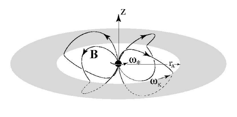
Figure 1.— Three-dimensional view of four field lines going from the star to the Alfvén radius $r_{A}$. For the conditions shown the disk angular velocity at $r_{A}$, $\omega_{K}(r_{A})$, is larger than the star’s angular velocity $\omega_{*}$.

From a statistical analysis of $24$ binary radio pulsars with nearly circular orbits and low mass companions, Van den Heuvel and Bitzaraki (1995) discovered a clear correlation between the spin period $P$ and the orbital period $P_{orb}$, as well as between the magnetic field and the orbital period. The pulsar period and magnetic field strength increase with the orbital period at $P_{orb}>100$ days, and scatters around $P\sim 3$ ms and $B\sim 2\times 10^{8}$ G for smaller binary periods. These relations strongly suggest that an increase in the amount of accreted mass leads to a screening of the initial magnetic field, and that there is a lowest field strength of about 10⁸ G. Magnetic field screening during accretion has been discussed by a number of authors (see, e.g., BK74; Romani 1990; Wijers 1997; Cheng & Zhang 1998, 2000; Choudhuri & Konar 2002; Payne & Melatos 2004). The studies by Cheng and Zhang and by Payne and Melatos analyze the flow and magnetic field evolution within the neutron star in contrast with the present work which is concerned mainly with the magnetosphere of the star.

Here we present an analytical model of the screening of the magnetic field of a rotating neutron star due to the accretion of plasma from a disk. The system is assumed to be axisymmetric. In the idealized case of a non-conducting sphere, the decrease of the external magnetic field occurs due to the electric current in the infalling plasma. The accretion of this current carrying plasma to the star’s surface creates an induced magnetic moment with a sign opposite to that of the original magnetic dipole. In the more realistic case where the star is treated as a conducting sphere, the magnetic field due to the accreted current-carrying plasma does not penetrate the main volume of the star. As a result the screening effect of the plasma is greatly reduced (compared with the case of a non-conducting star), and the time-scale for appreciable screening is greatly increased. For representative parameters we find that the magnetic field of the conducting star decreases significantly on a time-scale of the order of $10^{7}$ yr. The screening mechanism stops working when the Alfvén radius is comparable to the radius of the star.

In the §2 the general picture is described, and the main equations are derived. In §3 and §4 the magnetic field decrease during plasma accretion is considered for non-conducting and conducting spheres, respectively. We calculate the time-scale for an appreciable decrease of the magnetic field of a conducting star which depends on the radial thickness of the accreted matter. In §5 we estimate the thickness of the accreted matter and the time scale for the magnetic field to diffuse out of the star once accretion has ceased. In §6 we give the conclusions of this work.

2. Theory

We consider disk accretion to a rotating neutron star with an aligned dipole magnetic field as indicated in Figure 1. That is, we consider an axisymmetric star, magnetic field, and disk. Further, we consider configurations which are mirror symmetric about the equatorial plane. We use both spherical $(R,\theta,\phi)$ and cylindrical $(r,\phi,z)$ non-rotating coordinate systems.

For this system the corotation radius is

$$r_{cr}=\left({GM\over\omega_{*}^{2}}\right)^{1/3}\approx 1.7\times 10^{8}~{}P^{2/3}~{}{\rm cm}~{},$$ (1)

where, $\omega_{*}$ is the angular rotation rate of the star, $P=2\pi/\omega_{*}$ is its period, and the star’s mass is considered to be $1.4M_{\odot}$. The Alfvén radius $r_{A}$ (or inner radius) of the disk is the distance at which the kinetic energy density of the matter $\rho{\bf v}^{2}/2$ is comparable with the magnetic energy density ${\bf B}^{2}/8\pi$ (Ghosh & Lamb 1979). This gives

$$r_{A} \approx k_{A}\left({\mu^{2}\over\dot{M}\sqrt{GM}}\right)^{2/7}~{},$$ (2)

$$\approx 1.94\times 10^{8}\left({k_{A}\over 0.5}\right)\left({\mu_{30}^{2}\over\dot{M}_{-9}}\right)^{2/7}~{}{\rm cm}~{}.$$

Here, $\mu$ or $\mu_{30}\equiv\mu/(10^{30}$ G cm³) is the star’s magnetic moment, $\dot{M}$ or $\dot{M}_{-9}\equiv\dot{M}/(10^{-9}M_{\odot}/{\rm yr})$ is the mass accretion rate. The accretion luminosity is $L_{accr}=GM\dot{M}/R_{*}\approx 1.2\times 10^{37}\dot{M}_{-9}$ erg/s assuming the star’s radius $R_{*}=10^{6}$ cm, while the Eddington luminosity for a $1.4M_{\odot}$ star is $L_{Edd}\approx 1.76\times 10^{38}$ erg/s. Thus $L_{accr}/L_{Edd}=\approx 0.067\dot{M}_{-9}$. The dimensionless coefficient $k_{A}$ is of order of one-half and depends weakly on the disk parameters (see Ghosh & Lamb 1979; Lovelace, Romanova, & Bisnovatyi-Kogan 1995; Long, Romanova, & Lovelace 2004). The star’s accretion luminosity is $\dot{E}_{a}=GM\dot{M}/R_{*}\approx 1.2\times 10^{37}\dot{M}_{-9}$ erg/s with the star’s radius $R_{*}$ assumed to be $10^{6}$ cm.

The ratio $r_{A}/r_{cr}$ determines the qualitative evolution of the system. For $r_{A}\lesssim r_{cr}$, accretion causes the star to spin-up with the rate of increase angular momentum $dJ/dt\approx\dot{M}(GMr_{A})^{1/2}$, where $J=I\omega_{*}$, with $I=10^{45}I_{45}$ g cm² the star’s moment of inertia. On the other hand for $r_{A}\gtrsim r_{cr}$, the star spins-down with the rate $dJ/dt\approx-\dot{M}(GMr_{A})^{1/2}$. For $r_{cr}\ll r_{A}$ the star spins down but is in the propeller regime where an appreciable fraction of the accreting matter may be expelled from the system by the rotating magnetic field (Illarionov & Sunyaev 1975; Lovelace, Romanova, & Bisnovatyi-Kogan 1999) or the accretion to the star’s surface may be highly non-stationary (Romanova et al. 2004). In the propeller regime, the mass accretion rate in the outer disk ($\dot{M}$ in equation 2) may be substantially larger than the mass accretion rate to the surface of the star (Lovelace, et al. 1999). We consider only cases where $r_{A}>R_{*}$, with $R_{*}$ the star’s radius.

For distances $R$ less than $r_{A}$, the accreting matter moves in a funnel flow which follows approximately the dipole magnetic lines as sketched in Figure 2 (see, e.g., Romanova et al. 2002). For $R\ll r_{A}$ the velocity of the matter in the funnel flow is approximately free-fall. The cross sectional area of the funnel flow $S$ varies as $R^{3}$ for a dipole field so that $\rho\propto 1/R^{5/2}$. Consequently, $\rho{\bf v}^{2}/2$ varies as $1/R^{7/2}$. Thus the kinetic energy density of the funnel matter is much less that that of the magnetic field which varies as $1/R^{6}$. Therefore, the funnel flow is magnetically dominated or force-free for $R<r_{A}$.

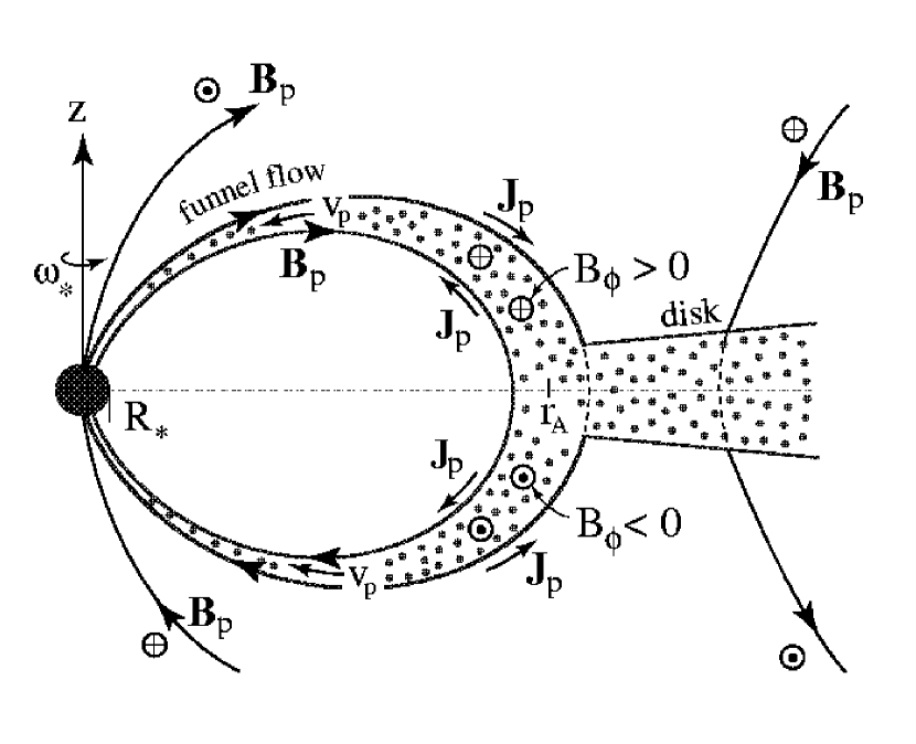
Figure 2.— Diagram of the poloidal cross-section of the accretion disk and funnel flow. ${\bf B}_{p}$ is the poloidal magnetic field, $B_{\phi}$ is the toroidal magnetic field, ${\bf J}_{p}$ the poloidal current density, and ${\bf v}_{p}$ is the poloidal component of the funnel flow velocity. The symbol $\odot$ represents an arrow out of the page, while $\oplus$ represents the opposite direction. The solid dots indicate a high plasma density.

For the considered axisymmetric system, the magnetic field has the form

$${\bf B}~{}={\bf B}_{p}+B_{\phi}\hat{{\hbox{\tenbg\char 30\relax}}~{}}~{},$$

with ${\bf B}_{p}=B_{R}{\hat{\bf R}}+B_{\theta}\hat{{\hbox{\tenbg\char 18\relax}}~{}}.$ We can write

$$B_{R}={1\over R^{2}\sin\theta}{\partial\Psi\over\partial\theta}~{},\quad B_{\theta}=-~{}{1\over R\sin\theta}{\partial\Psi\over\partial R}~{},$$

where $\Psi(R,\theta)\equiv R\sin\theta A_{\phi}(R,\theta)$ is referred to as the ‘flux function.’ Note that $\Psi(R,\theta)=$ const is the equation for the poloidal projection of a magnetic field line.

In the force-free limit, the flow speeds are sub-Alfvénic, ${\bf v}^{2}\ll{v}_{A}^{2}={\bf B}^{2}/4\pi\rho$, where $v_{A}$ is the Alfvén velocity. In this limit, ${\bf J\times B}\approx 0$; therefore, ${\bf J}=\lambda{\bf B}$ (Gold & Hoyle 1960). Because ${\bf\nabla\cdot J}=0$, $({\bf B\cdot\nabla})\lambda=0$ and consequently $\lambda=\lambda(\Psi)$. Thus, Ampère’s equation becomes ${\bf\nabla\times B}={4\pi\lambda(\Psi)}{\bf B}/c$. The $R$ and $\theta$ components of Ampère’s equation imply

$$H(\Psi)=R\sin\theta B_{\phi}~{},\quad{\rm and}\quad{dH\over d\Psi}={4\pi\over c}\lambda(\Psi)~{},$$

where $H(\Psi)$ is another function of $\Psi$. Thus, $H(\Psi)=$ const along any given field line, and ${\bf J}_{p}=(c/4\pi)(dH/d\Psi){\bf B}_{p}$ so that $({\bf J}_{p}\cdot{\bf\nabla})H=0$. The toroidal component of Ampère’s equation gives

$$\Delta^{\star}\Psi=-H(\Psi){dH(\Psi)\over d\Psi}~{},$$ (3)

where

$$\Delta^{\star}\equiv{\partial^{2}\over\partial R^{2}}+{1-\zeta^{2}\over R^{2}}{\partial^{2}\over\partial\zeta^{2}}~{},$$

and $\zeta\equiv\cos\theta$. This is the Grad-Shafranov equation for $\Psi$ (see e.g. Lovelace et al. 1986). Note that the lines $\Psi(R,\theta)=$const are the poloidal magnetic field lines. Alternatively the rotation of such a line around the $z-$axis form a flux surface.

The magnetic moment of the star,

$${\hbox{\tenbg\char 22\relax}}={1\over 2c}\int_{R\leq R_{*}}d^{3}x~{}{\bf r}\times{\bf J}=\mu~{}\hat{\bf z}$$

where

$$\mu={\pi\over c}\int_{0}^{R_{*}}R^{3}dR~{}\int_{0}^{\pi}d\theta\sin^{2}\theta~{}J_{\phi}~{}.$$ (4)

Initially, before there has been appreciable accretion, we assume that the magnetic moment $\mu_{i}=\mu(t=0)$ is due to current flow deep inside the star. Thus the star’s initial magnetic field is given by $\Psi_{i}(R,\theta)=\mu_{i}\sin^{2}\theta/R$ for $R\geq R_{*}$. Note that $\Delta^{*}\Psi_{i}=0$.

In the following we show that accretion of current carrying matter to the surface of the star acts to reduce the star’s magnetic moment. We consider first the case of a non-conducting star in §3. In §4 we consider the realistic case of a highly conducting star.

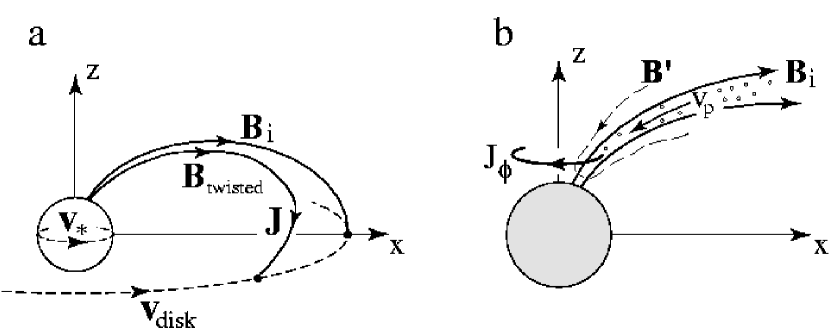
Figure 3.— (a) Schematic drawing of an initial dipole field line ${\bf B}_{i}$ (in the $x,z$ plane) and the corresponding twisted field line for the case where the angular velocity of the disk at the Alfvén radius $\omega_{K}(r_{A})$ is less than the angular velocity of the star $\omega_{*}$. This is opposite to the case shown in Figures 1 and 2. The current flow ${\bf J}$ parallel to the ${\bf B}$-field necessary to produce this twist is into the star at high latitudes and out of the star at low latitudes. The low-latitude current flow has the dominant screening effect and only this current is shown in (${\bf a}$). This current flow along the twisted field line gives rise to a negative toroidal current density $J_{\phi}$ near the star as shown in ($({\bf b}$). Panel (b) shows the poloidal field component ${\bf B}^{\prime}$ arising from the toroidal current $J_{\phi}$. The funnel flow is indicated by the small circles and the arrow ${\bf v}$ indicates the flow velocity.

3. Accretion to a Non-Conducting Star

This subsection treats the case of a non-conducting star in order to explain our model of the magnetosphere. This model star has a non-varying dipole field source at its center. The magnetic field associated with the accreting matter is allowed to penetrate the star’s surface $R=R_{*}$.

The accreting plasma outside the star is highly conducting. Consequently, plasma falling onto the star carries with it an embedded magnetic field and the associated current density as sketched in Figures 2 and 3. This plasma infall causes the star’s magnetic moment to change at the rate

$${d\mu\over dt}={\pi\over c}R_{*}^{3}\int_{0}^{\pi}d\theta\sin^{2}\theta~{}\big{(}J_{\phi}v_{R}\big{)}_{R_{*}+0}~{}.$$ (5)

Here, $R_{*}+0$ indicates a distance just outside of the star, and $v_{R}$ is the plasma infall speed which is approximately the free-fall speed $v_{R*}=(2GM/R_{*})^{1/2}$, because the star’s radius $R_{*}$ is considered to be significantly smaller than the Alfvén radius $r_{A}$. This speed is much larger than the rotational velocity of the star’s surface $\sim\omega R_{*}$, because the corotation radius is also considered to be significantly larger than $R_{*}$. We assume that there is a strong shock just outside the star’s surface which thermalizes the bulk kinetic energy of the flow.

The total magnetic field $\Psi=\Psi_{s}+\Psi_{m}$ is the sum of the field due to the star, $\Psi_{s}$, and that due to current flow in the magnetosphere, $\Psi_{m}$. For the considered conditions where $R_{*}\ll r_{A}$, we show below that $|\Psi_{m}|\ll\Psi_{s}$. We have $\Psi_{s}=\mu\sin^{2}\theta/R$ far from the star, which satisfies the $\Delta^{*}\Psi_{s}=0$. Consequently, equation (3) gives $\Delta^{*}\Psi_{m}=-H(\Psi_{s})dH(\Psi_{s})/d\Psi_{s}$. Because $\Psi_{m}$ is small, $\Psi$ (without the $s$ subscript) in subsequent analysis refers to the field of the star.

The funnel flow as shown in Figure 2 exists close to the flux surface $\Psi=\Psi_{ff}=\mu/r_{A}$. For a dipole field the funnel flow hits the star’s surface at $\theta_{ff}\approx(R_{*}/r_{A})^{1/2}$. The width in $\Psi$ of the funnel flow is $\Delta\Psi_{ff}/\Psi_{ff}\approx\Delta r_{A}/r_{A}\ll 1$. The radial width is assumed to be of the order of the half-thickness of the disk $h_{A}$ at the Alfvén radius $r_{A}$ as indicated by MHD simulations of funnel flows by Romanova et al. (2002). It is clear that $H(\Psi)$ is zero outside of the funnel flow and that $H^{2}$ is a maximum $H_{m}^{2}$ in the middle of the funnel flow at $\Psi=\Psi_{ff}$. The value of $H_{m}^{2}$ is estimated by the condition that $B_{\phi}^{2}\approx B_{p}^{2}$ at the Alfvén radius $r_{A}$. For larger values of $(B_{\phi}/B_{p})^{2}$ at $r_{A}$, the magnetic field loop would open (Lynden-Bell & Boily 1994; Lovelace, Romanova, & Bisnovatyi-Kogan 1995). Thus $H_{m}^{2}\approx\mu^{2}/r_{A}^{4}$. This value can be used to show that $|\Psi_{m}|/\Psi_{s}\approx(R_{*}/r_{A})^{4}\ll 1$.

In equation (5) we can use the fact that

$$J_{\phi}={c\over 4\pi R\sin\theta}~{}{d\over d\Psi}{H^{2}\over 2}~{}.$$ (6)

Thus

$${d\mu\over dt}={1\over 4}R_{*}^{2}~{}v_{R*}\int_{0}^{\pi/2}d\theta~{}\sin\theta~{}{dH^{2}\over d\Psi}\bigg{|}_{R_{*}+0}~{},$$ (7)

where we have combined the contributions of the two hemispheres. On the star’s surface we have $\Psi=\mu\sin^{2}\theta/R_{*}$ so that $\cos\theta=(1-R_{*}\Psi/\mu)^{1/2}$. Thus we obtain

$${d\mu\over dt}={R_{*}^{3}v_{R*}\over 8\mu}\int_{0}^{\mu/R_{*}}{d{\Psi}\over(1-R_{*}{\Psi}/\mu)^{1/2}}~{}{dH^{2}\over d{\Psi}}~{}.$$ (8)

The square root can be Taylor expanded in that $R_{*}{\Psi}/\mu\approx R_{*}/r_{A}$. An integration by parts then gives

$${d\mu\over dt}=-~{}{R_{*}^{4}v_{R*}\over 16\mu^{2}}\int_{0}^{\mu/R_{*}}d{\Psi}~{}H^{2}~{}.$$ (9)

Thus the star’s magnetic moment decreases independent of the sign of $H$ and hence independent of the sign of $\omega_{K}(r_{A})-\omega_{*}$.

Using the mentioned estimates $H_{m}^{2}\approx\mu^{2}/r_{A}^{4}$ and $\Delta\Psi_{ff}\approx(h_{A}/r_{A})\Psi_{ff}=(h_{A}/r_{A})(\mu/r_{A})$, equation (9) gives

$${d\mu\over dt}=-~{}{1\over 16}~{}\mu\left({R_{*}\over r_{A}}\right)^{4}\left({h_{A}\over r_{A}}\right)\left({v_{R*}\over r_{A}}\right)~{}.$$ (10)

This equation is not realistic for a neutron star which is highly conducting.

4. Accretion to Conducting Star

We now treat the case of a highly conducting star. For $R\leq R_{*}$ the star is considered to be perfectly conducting with the frozen in dipole magnetic field $\Psi_{i}=\mu_{i}\sin^{2}\theta/R$. The magnetic field associated with the accreting matter cannot penetrate the surface $R=R_{*}$. The shell from $R=R_{*}$ to $R_{a}>R_{*}$ is the layer of accreted matter. The layer thickness is $R_{a}-R_{*}=\Delta R_{a}\ll R_{*}$. The accumulated azimuthal current carried by the accretion layer is modeled by surface current layer ${\cal K}_{\phi}(\theta)$ at $R_{\cal K}=R_{*}+\Delta R_{a}/2$.

The magnetic field in the different radial regions can be expanded in terms of solutions of $\Delta^{*}\Psi=0$, because the contribution of the magnetospheric currents is negligible. For the region $R>R_{\cal K}$ we have

$$\Psi^{+}=\Psi_{i}(R,\zeta)+\sum_{n=1,3,..}a_{n}{G_{n}(\zeta)\over R^{n}}~{},$$ (11)

where $G_{n}(\zeta)$ is a Gegenbauer polynomial, $\zeta\equiv\cos\theta$, and the $a_{n}$ are coefficients determined below. The terms with even values of $n$ are excluded because they correspond to a field which is not mirror symmetric about the $z=0$ plane. We can take

$$G_{n}(\zeta)=(1-\zeta^{2}){dP_{n}(\zeta)\over d\zeta}~{},$$ (12)

where $P_{n}(\zeta)$ is the usual Legendre polynomial. The other solutions related to the Legendre $Q_{n}$ functions are unphysical. One can readily show that the $G_{n}$ obey the orthogonality relations

$$\int_{-1}^{1}d\zeta~{}{G_{n}(\zeta)G_{m}(\zeta)\over 1-\zeta^{2}}={2n(n+1)\over 2n+1}~{}\delta_{nm}~{}.$$ (13)

For example,

$$G_{1}=1-\zeta^{2}~{},$$

$$G_{3}=-{3\over 2}+9\zeta^{2}-{15\over 2}\zeta^{4}~{},$$

and

$$G_{5}={15\over 8}-{225\over 8}\zeta^{2}+{525\over 8}\zeta^{4}-{315\over 8}\zeta^{6}~{}.$$

As $\zeta^{2}\rightarrow 1$, $G_{n}\rightarrow n(n+1)(1-\zeta^{2})/2$. As $\zeta\rightarrow 0$ (the equatorial plane), $G_{n}\rightarrow\sin(\pi n/2)n(n-2)!!/(n-1)!!$, with values of $1,-3/2,$ and $15/8$ for $n=1,3,$ and $5$.

For $R_{*}\leq R<R_{\cal K}$, we have

$$\Psi^{-}=\Psi_{i}(R,\zeta)+\sum_{n=1,3,..}b_{n}\left({1\over R^{n}}-{R^{n+1}\over R_{*}^{2n+1}}\right)G_{n}(\zeta)~{},$$ (14)

so that $\Psi(R_{*},\zeta)=\Psi_{i}(R,\zeta)$. For $R\leq R_{*}$, $\Psi=\Psi_{i}(R,\zeta)$.

Matching the inner and outer flux functions at $R=R_{\cal K}$ gives

$$a_{n}=b_{n}\left[1-\left({R_{\cal K}\over R_{*}}\right)^{2n+1}\right]~{}.$$ (15)

Evaluation of the jump across the $R=R_{\cal K}$ surface gives

$$\left({\partial\Psi^{+}\over\partial R}-{\partial\Psi^{-}\over\partial R}\right)_{R_{\cal K}} = -\sum_{n=1,3,..}a_{n}~{}{G_{n}(\zeta)\over R_{\cal K}^{n+1}}~{}{2n+1\over 1-\beta^{2n+1}}~{},$$ (16)

$$= -{4\pi R_{\cal K}\sin\theta\over c}{\cal K}_{\phi}(\zeta)~{},$$

where $\beta\equiv R_{*}/R_{\cal K}<1$, and ${\cal K}_{\phi}(\zeta)$ is the mentioned surface current density. Thus we obtain

$$a_{n}={4\pi R_{\cal K}^{n+2}\over c}~{}{1-\beta^{2n+1}\over 2n(n+1)}\int_{-1}^{1}d\zeta~{}{{\cal K}_{\phi}(\zeta)G_{n}(\zeta)\over(1-\zeta^{2})^{1/2}}~{}.$$ (17)

Note that $a_{1}$ is the contribution to the star’s dipole moment due to the surface current ${\cal K}_{\phi}$, and $a_{3}$ is related to the quadrupole moment due to ${\cal K}_{\phi}$. Note also that $1-\beta^{2n+1}\approx(2n+1)(\Delta R_{a}/R_{*})/2$ which is justified subsequently.

From the considerations of §3, we have

$${d{\cal K}_{\phi}\over dt}=\big{(}J_{\phi}v_{R}\big{)}_{R_{a}}~{},$$ (18)

where $J_{\phi}$ is given by equation (6). Thus we find

$${da_{n}\over dt}={R_{*}^{n+1}v_{R*}\over 4n(n+1)}(1-\beta^{2n+1})\int_{-1}^{1}d\zeta~{}{dP_{n}\over d\zeta}{dH^{2}\over d\Psi}\bigg{|}_{R_{a}}~{},$$ (19)

In particular,

$${da_{1}\over dt}={1\over 4}{R_{*}^{2}v_{R*}}(1-\beta^{3})\int_{0}^{\pi/2}d\theta~{}\sin\theta~{}{dH^{2}\over d\Psi}\bigg{|}_{R_{a}}~{},$$ (20)

which differs from equation (7) by the factor $1-\beta^{3}$. Note that we have neglected the gradual variation of the thickness $\Delta R_{a}$ of the accretion layer. This is justified in §5.

It is useful in subsequent work to introduce

$$A_{1}\equiv\mu_{i}+a_{1}~{},\quad A_{n}\equiv a_{n}/R_{*}^{n-1}~{},~{}~{}n=3,5,..$$ (21)

because the $A_{n}^{\prime}s$ all have the same dimensions as the dipole moment.

4.1. Magnetic Energy

The magnetic energy of the system is

$$W = {1\over 8\pi}\int d^{3}x~{}({\bf B}_{i}+{\bf B}^{\prime})^{2}=W_{i}+W^{\prime},$$

$$W^{\prime} = {1\over 8\pi}\int d^{3}x~{}({\bf B}^{\prime})^{2}~{}.$$ (22)

Here, ${\bf B}_{i}$ is the initial dipole field and $W_{i}$ the associated magnetic energy which is independent of time. Further, ${\bf B}^{\prime}(t)$ is the field due to the currents on the surface of the star which result from the accretion and $W^{\prime}$ is the associated magnetic energy. The cross term involving ${\bf B\cdot B}^{\prime}$ in the first line of the equation vanishes because in the volume in which ${\bf B}^{\prime}$ is non-zero ($R\geq R_{*}$), ${\bf B}_{i}$ can be written as the gradient of a potential. We can also write

$$W^{\prime}={1\over 2c}\int d^{3}x~{}J_{\phi}^{\prime}A_{\phi}^{\prime}~{}.$$

Using equation (16) and equation (13) then gives

$$W^{\prime}={1\over R_{*}^{3}}{R_{*}\over\Delta R_{a}}\sum_{n=1,3,..}{n(n+1)\over(2n+1)^{2}}~{}(A_{n}-\mu_{i}\delta_{n0})^{2}~{},$$ (23)

where $\delta_{n0}$ is the Kronecker delta. We have made the approximation $1-\beta^{2n+1}\approx(2n+1)(\Delta R_{a}/R_{*})/2$, which is justified below where we estimate $\Delta R_{a}$.

Most of the magnetic energy $W^{\prime}$ is in the accretion layer on the star’s surface. The reason for this is indicated by the schematic drawing in Figure 3 of the fields ${\bf B}_{i}$ and ${\bf B}^{\prime}$. The magnetic energy of the ${\bf B}^{\prime}$ field outside of the star ($R\geq R_{a}$) is

$$W^{\prime}({\rm ext}) = {1\over 4}\int_{-1}^{1}d\zeta\int_{R_{a}}^{\infty}R^{2}dR~{}\left[(B_{R}^{\prime})^{2}+(B_{\theta}^{\prime})^{2}\right]$$ (24)

$$= {1\over R_{*}^{3}}\sum_{n=1,3,..}{n^{2}(n+1)\over 2(2n+1)}~{}(A_{n}-\mu_{i}\delta_{n0})^{2},$$

where we have replaced $R_{a}$ by $R_{*}$ because $\Delta R_{a}\ll R_{*}$. Retaining only the $n=1$ terms gives $W^{\prime}({\rm ext})/W^{\prime}=3\Delta R_{a}/(2R_{*})\ll 1$.

The ‘buried’ magnetic field is predominantly parallel to the star’s surface as indicated by Figure 3. The magnetic energy $W^{\prime}$ of the buried field, denoted $B^{\prime}_{\parallel}$, is approximately equal to $4\pi R_{*}^{2}\Delta R_{a}(B_{\parallel}^{\prime})^{2}/8\pi$. Retaining only the $n=1$ term in equation (23) gives the estimate

$$B_{\parallel}^{\prime}\sim{2\over 3}{R_{*}\over\Delta R_{a}}{|A_{1}-\mu_{i}|\over R_{*}^{3}}~{}.$$ (25)

The buried field strength is enhanced over the initial dipole field ($\mu_{i}/R_{*}^{3}$) by a factor $\approx R_{*}/\Delta R_{a}$ for $|A_{1}|\ll\mu_{i}$.

4.2. Field at Large Distances from Star

For large $R$,

$$\Psi={A_{1}G_{1}(\zeta)\over R}+{A_{3}G_{3}(\zeta)R_{*}^{2}\over R^{3}}+...$$ (26)

In the equatorial plane ($\zeta=0$),

$$\Psi(R,\pi/2)={A_{1}\over R}-{3A_{3}R_{*}^{2}\over 2R^{3}}+..,$$ (27)

where $A_{1}=\mu_{i}+a_{1}$ is the dipole moment at time $t$. We assume here and subsequently that the decrease in the dipole moment is limited in the respect that

$$A_{1}\gg{3|A_{3}|R_{*}^{2}\over 2r_{A}^{2}}~{},$$ (28)

and $A_{1}\gg|A_{n}G_{n}(0)|(R_{*}/r_{A})^{n-1}$ for $n=5,7,..$

Of course, the Alfvén radius $r_{A}$ depends on the magnetic field in the equatorial plane. This field is

$$B_{\theta}(R,\pi/2)=-{A_{1}\over R^{3}}+{9A_{3}R_{*}^{2}\over 2R^{5}}+...$$ (29)

Owing to inequality (28), $|B_{\theta}(r_{A},\zeta=0)|=|A_{1}|/r_{A}^{3}$ to a good approximation. For simplicity, we consider that $r_{A}$ depends only on $\mu$ or $A_{1}$ and that the other quantities in equation (2) such as $\dot{M}$ are constant. We then have

$$r_{A}=r_{Ai}\left({A_{1}\over\mu_{i}}\right)^{4/7}~{},$$ (30)

where $r_{Ai}$ is the Alfvén radius at time $t=0$. Inequality (28) can then be rewritten as

$${A_{1}\over\mu_{i}}\gg\left|{A_{3}\over\mu_{i}}\right|^{7/15}\left({R_{*}\over r_{Ai}}\right)^{14/15}~{}.$$ (31)

Owing to this inequality,

$$\Psi_{ff}={\mu_{i}\over r_{Ai}}\left({A_{1}\over\mu_{i}}\right)^{3/7}~{}.$$ (32)

We assume that $h_{A}/r_{A}=$ const $\ll 1$, so that $\Delta\Psi_{ff}/\Psi_{ff}=h_{Ai}/r_{Ai}$ = const $\ll 1$. From §3 we have $H_{m}=A_{1}^{2}/r_{A}^{4}$. Thus,

$$H_{m}^{2}={\mu_{i}^{2}\over r_{Ai}^{4}}\left({\mu_{i}\over A_{1}}\right)^{2/7}~{}.$$ (33)

4.3. Dimensionless Variables

It is natural to measure the magnetic moment $A_{1}$ in units of its initial value $\mu_{i}$,

$$\tilde{A}_{1}\equiv{A_{1}\over\mu_{i}}~{},\quad{\rm and}\quad\tilde{A}_{n}\equiv{A_{n}\over\mu_{i}}~{},~{}n=3,5,..$$ (34)

with the tildes indicating the dimensionless variables. We measure $\Psi$ in units of $\mu_{i}/R_{*}$, and $B_{R}(R_{*},\zeta)$ in units of $\mu_{i}/R_{*}^{3}$. In terms of the dimensionless variables, $\tilde{B}_{R}(R_{*},\zeta)=-d\tilde{\Psi}/d\zeta$. Further we have

$$\tilde{\Psi}_{ff}={R_{*}\over r_{Ai}}~{}\tilde{A}_{1}^{3/7}~{},\quad{\rm and}\quad\Delta\tilde{\Psi}_{ff}={R_{*}\over r_{Ai}}{h_{Ai}\over r_{Ai}}~{}\tilde{A}_{1}^{3/7},$$ (35)

from equation (35).

In subsequent work we drop the tilde’s from the $A_{n}^{\prime}s$ and the $\Psi^{\prime}s$.

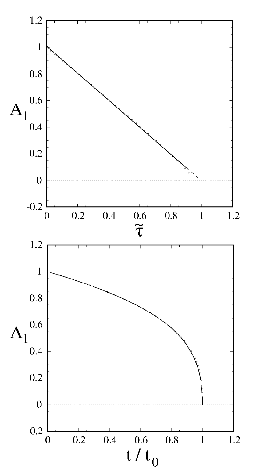
Figure 4.— Time dependence of the normalized magnetic moment $A_{1}/\mu_{i}$ for the special case of only the dipole mode. Here, $\mu_{i}$ is the initial magnetic moment of the star, and $t_{0}$ is given by equation (43).

4.4. Specific Model for $H(\Psi)$

The qualitative dependence of $H(\Psi)$ is discussed in §3. A specific function with this dependence is

$$\big{[}H(\Psi)\big{]}^{2}=H_{m}^{2}\exp\left(-{(\Psi-\Psi_{ff})^{2}\over 2\Delta\Psi_{ff}^{2}}\right)~{}.$$ (36)

We can now rewrite equation (19) in dimensionless form as

$${d{A}_{n}\over d\tau}=-{2n+1\over n(n+1)}~{}{{\cal I}_{n}\over{A}_{1}^{5/7}}~{}.$$ (37)

Here,

$${\cal I}_{n}\equiv\int_{0}^{1}d\zeta~{}{dP_{n}\over d\zeta}X\exp\left(-{X^{2}\over 2}\right),\quad X(\zeta)\equiv{\Psi(\zeta)-\Psi_{ff}\over\Delta\Psi_{ff}},$$

where $\Psi(\zeta)\equiv\Psi(R_{*},\zeta)$, with

$$\Psi(\zeta)=\sum_{n=1,3,..}A_{n}G_{n}(\zeta)~{}.$$

The dimensionless time variable $\tau$ is given by

$${dt\over d\tau}={4}\left({r_{Ai}\over R_{*}}\right)^{3}{R_{*}\over v_{R*}}~{}{\Delta\Psi_{ff}\over\Psi_{ff}}~{}{R_{*}\over\Delta R_{a}(t)}~{}.$$ (38)

The initial conditions for equations (37) are $A_{1}(0)=1$ and $A_{n}(0)=0$ for $n=3,5,..$.

For simplicity, we consider $\Delta\Psi_{ff}/\Psi_{ff}$ to be a fixed number small compared with unity. Consequently, the solution of equation (37) depends on the dimensionless time $\tau$ and on two dimensionless parameters, ${\cal E}$ and $\epsilon$,

$$A_{n}=A_{n}(\tau,{\cal E},\epsilon)~{},\quad{\cal E}\equiv{R_{*}\over r_{Ai}}~{},\quad\epsilon\equiv{\Delta\Psi_{ff}\over\Psi_{ff}}={h_{Ai}\over r_{Ai}}~{},$$ (39)

where ${\cal E}\ll 1$ and $\epsilon\ll 1$.

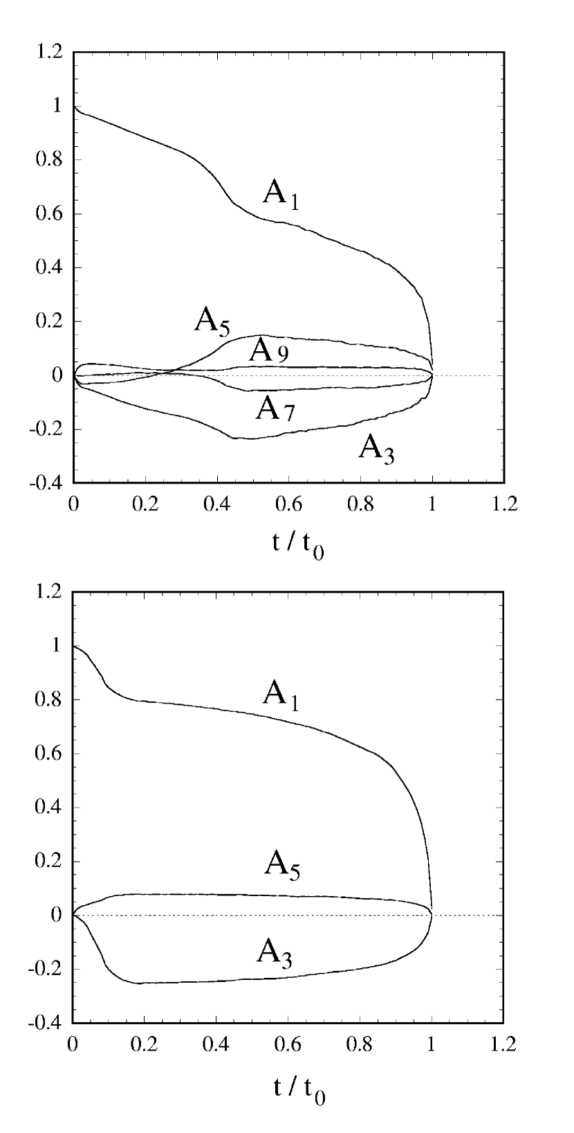
Figure 5.— Time dependence of the normalized magnetic multipole moments. The top panel is for a case with five modes for ${\cal E}=0.05$ and $\epsilon=0.1$, while the bottom panel is for three modes for ${\cal E}=0.025$ and $\epsilon=0.05$. The time $t_{0}$ is given by equation (51).

4.5. Single Mode, $A_{1}\neq 1$

For the special case of only one mode $A_{1}\neq 0$, equation (37) can be approximated analytically. We find

$${\cal I}_{1}=-{A_{1}^{4/7}\over\epsilon~{}{\cal E}}\int_{0}^{1}d\zeta~{}(\zeta^{2}-Z)\exp[-k(\zeta^{2}-Z)^{2}]~{}.$$ (40)

Here, $k\equiv A_{1}^{8/7}/(2\epsilon^{2}{\cal E}^{2})$ and $Z\equiv 1-{\cal E}/A_{1}^{4/7}$, where we assume that $Z>0$ or $A_{1}>{\cal E}^{7/4}$. Because $\epsilon\ll 1$, $k\gg 1$ so that equation (40) can be evaluated easily as

$${\cal I}_{1}\approx-{\sqrt{\pi/2}\over 2}{\epsilon^{2}{\cal E}^{2}\over A_{1}^{8/7}Z^{3/2}}~{}.$$ (41)

Thus we find

$${dA_{1}\over d\tilde{\tau}}=-1~{},\quad{\rm or}\quad A_{1}=1-\tilde{\tau}~{},~{}0\geq\tilde{\tau}\leq 1~{},$$

$${dt\over d\tilde{\tau}}={16\sqrt{2}\over 3\sqrt{\pi}}~{}{A_{1}^{13/7}\over\epsilon~{}{\cal E}^{5}}~{}{R_{*}\over v_{R*}}~{}{R_{*}\over\Delta R_{a}}~{}.$$ (42)

We have used the approximation $Z=1$ which assumes $A_{1}\gg{\cal E}^{7/4}\ll 1$.

Equation (42) can be solved to give

$$t=t_{0}[1-(1-\tilde{\tau})^{20/7}]~{}.$$

Here,

$$t_{0}={28\sqrt{2}\over 15\sqrt{\pi}}~{}{R_{*}\over v_{R*}}~{}{1\over\epsilon~{}{\cal E}^{5}}~{}{R_{*}\over<\!\!\Delta R_{a}\!>}~{},$$ (43)

is the time-scale for the field decrease. This equation can also be written as

$$t_{0}\approx 1.5~{}{R_{*}\over v_{R*}}~{}{r_{Ai}\over h_{Ai}}\left({r_{Ai}\over R_{*}}\right)^{5}{R_{*}\over<\!\!\Delta R_{a}\!>}~{}.$$

Here, $<\!\!\Delta R_{a}\!\!>$ is the time-averaged thickness of the accretion layer where it is assumed that $\Delta R_{a}$ varies gradually with time. For a neutron star of mass $M=1.4M_{\odot}$ and radius $R_{*}=10^{6}$ cm, we find

$$t_{0}\approx 0.78\times 10^{5}\left({0.001\over\epsilon}\right)\left({0.005\over{\cal E}}\right)^{5}\left({100\over R_{*}/<\!\!\Delta R_{a}\!\!>}\right)~{}{\rm yr}~{}.$$ (44)

The normalization of ${\cal E}$, or equivalently $r_{Ai}$, follows from equation (2). The normalization of $\epsilon$, or equivalently $h_{Ai}/r_{Ai}$, is based on the Shakura-Sunyaev disk model (1973) which indicates that $\epsilon$ depends quite weakly on the different parameters (e.g., $\epsilon\propto\dot{M}^{1/5}$). The normalization of $R_{*}/<\!\!\Delta R_{a}\!\!>$ is discussed in §5. The shortness of this time-scale is due to the fact that only one mode is accounted for.

4.6. Numerical Integrations

The results of §4.5 for a single mode point up the importance of using a new time variable in place of $\tau$ in equation (37). That is, we rewrite this equation as

$${d{A}_{n}\over d\tau^{\prime}}=-{2n+1\over n(n+1)}~{}A_{1}^{8/7}(\tau^{\prime})~{}{{\cal I}_{n}(\tau^{\prime})}~{},$$ (45)

for $n=1,3,..$, where

$${d\tau\over d\tau^{\prime}}=A_{1}^{13/7}(\tau^{\prime})~{}.$$ (46)

Combining this equation with equation (38) gives

$${dt\over d\tau^{\prime}}=4~{}{\epsilon\over{\cal E}^{3}}~{}{R_{*}\over v_{R*}}~{}{R_{*}\over<\!\Delta R_{a}\!>}~{}A_{1}^{13/7}~{}.$$ (47)

We let $\tau_{0}$ and $\tau_{0}^{\prime}$ denote the values for which $A_{1}\leq 0.01$. We have

$$\tau_{0}=\int_{0}^{\tau_{0}^{\prime}}d\tau^{\prime}A_{1}^{13/7}(\tau^{\prime})~{}.$$ (48)

The corresponding actual time when $A_{1}\leq 0.01$ is

$$t_{0}=4~{}{\epsilon\over{\cal E}^{3}}~{}{R_{*}\over v_{R*}}~{}{R_{*}\over<\!\Delta R_{a}\!>}~{}\tau_{0}({\cal E},\epsilon)~{}.$$ (49)

For the case of a single mode ($A_{1}$), $\tau^{\prime}$ is proportional to $\tilde{\tau}$ (neglecting the weak time dependence of $\Delta R_{a}$). For this case $A_{1}$ decreases linearly with $\tilde{\tau}$ or $\tau^{\prime}$.

We find equations (45) to be stiff. For this reason a predictor-corrector code (Gear 1971) was developed and used to solve the equations for $1,~{}3,$ and $5$ modes. The integrals ${\cal I}_{n}$ were evaluated using a stretched $\zeta$ grid with $10^{4}-10^{5}$ points. Figure 4 shows the numerical solution for the case of one mode ($A_{1}$). This agrees closely with the analytic solution of §4.5.

Figure 5 shows sample results for cases of three and five modes. The time-scales $t_{0}({\cal E},\epsilon)$ for three and five modes are not appreciably different. Combining the results of many runs for ${\cal E}=0.01-0.1$ and $\epsilon=0.02-0.1$ we find

$$\tau_{0}\approx{1.2\times 10^{-4}\over{\cal E}^{3.6}~{}\epsilon^{2.7}}~{}.$$ (50)

The integrations become increasingly long as $\epsilon$ and ${\cal E}$ decrease. In view of equation (49) we have

$$t_{0}\approx 1.6\times 10^{7}\left({0.001\over\epsilon}\right)^{1.7}\left({0.005\over{\cal E}}\right)^{6.6}\left({100\over R_{*}/<\!\!\Delta R_{a}\!\!>}\right)~{}{\rm yr}~{}.$$ (51)

This time-scale is considerably longer than that for the case of the single mode (equation 44). The time-scale varies approximately as $\mu_{i}^{3.8}/\dot{M}^{1.9}$. Thus for a neutron star with an initial surface magnetic field of $2\times 10^{12}$ G or $\mu_{i}=2\times 10^{30}$ Gcm³, the time-scale of equation (51) increases to $2.2\times 10^{8}$ yr.

Figure 6 shows the magnetic field lines at a time during the evolution and the initial, pure dipole field. Figure 7 shows the corresponding surface current density on the star’s surface.

5. Accretion Layer Thickness

We now give a rough estimate the accretion layer thickness $\Delta R_{a}$. We let $\Delta M$ denote the mass accreted after time $t$, which is in a layer of thickness $\Delta R_{a}\ll R_{*}$. The mean density of the layer is thus $\bar{\rho}\sim\Delta M/(4\pi R_{*}^{2}\Delta R_{a})$. The change in pressure across the layer in hydrostatic equilibrium is $p\sim[\Delta M/(4\pi R_{*}^{2})]g$, where $g=GM/R_{*}^{2}\approx 1.87\times 10^{14}$ cm/s². The equation of state of the neutron star matter gives $p\approx k(\bar{\rho})^{n}$ with $k\approx 2.1\times 10^{11}$ cgs, and $n\approx 1.5$ (Baym, Bethe, & Pethick 1971). Thus we obtain

$$\Delta R_{a} \sim \left({k\over g}\right)^{1/n}\left({\Delta M\over 4\pi R_{*}^{2}}\right)^{(n-1)/n}$$ (52)

$$\sim 1.3\times 10^{4}\left({\Delta M\over 10^{-2}M_{\odot}}\right)^{1/3}~{}{\rm cm}~{}.$$

For $\Delta R_{a}=10^{4}$ cm, equation (25) gives an estimate of the buried magnetic field of $\sim 6.7\times 10^{13}$ G. Thus the magnetic pressure in the accretion layer is negligible compared the matter pressure.

5.1. Ohmic Diffusion of the Field

The influence of Ohmic diffusion on the ‘burial’ of magnetic field during accretion to a neutron star has been studied by Cumming, Zweibel, and Bildsten (2001). They treat the competition between the inward advection of the magnetic field inside the star and the tendency of the field to diffusion outward due to the finite conductivity of the plasma. For sufficiently large accretion rates (such as that considered here) the inward advection is found to be larger than the diffusion.

Magnetic field buried during intensive accretion will Ohmically diffuse out of the star after the accretion stops (BK74). The time scale for the buried field to diffuse out of the star can be estimated as

$$t_{Ohm}\sim{(\Delta R_{a})^{2}\over\eta}~{},\quad\quad\eta={c^{2}\over 4\pi\sigma}~{},$$ (53)

where $\eta$ is the magnetic diffusivity, and $\sigma$ is the conductivity. Using Cumming et al.’s §2.2 formula for the conductivity and our normalization values we find

$$t_{Ohm}\sim 2.7\times 10^{9}\left({\Delta R_{a}\over 10^{4}{\rm cm}}\right)\left({\Delta M\over 10^{-2}M_{\odot}}\right)~{}{\rm yr}~{}.$$ (54)

Thus it takes a rather long time for the field to diffuse out of the star.

It is possible that the buried magnetic field is subject to the interchange or buoyancy instabilities considered by Cumming et al. (2001), and by Kato, Fukue, and Mineshige (1998), but the detailed analysis is beyond the scope of the present work.

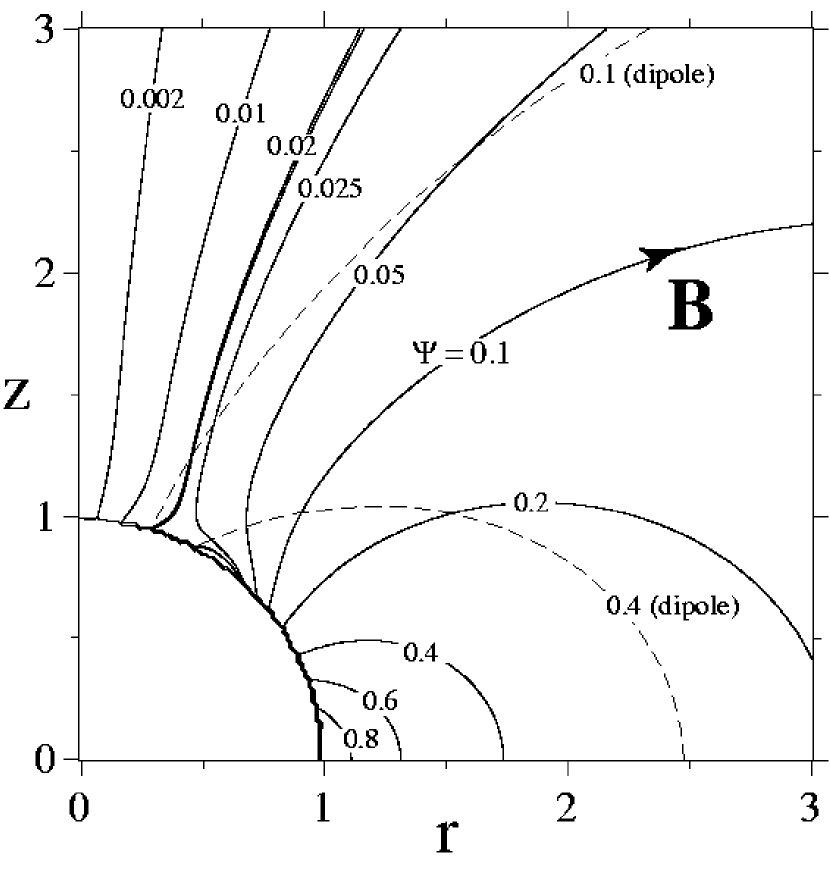
Figure 6.— Magnetic field lines of a screened star (solid lines) with three modes at $t/t_{0}=0.85$ when $A_{1}\approx 0.59$, $A_{3}\approx-0.19$, and $A_{5}\approx 0.062$ for a case with ${\cal E}=0.025$ and $\epsilon=0.025$. The dashed lines are for the initial, pure dipole field. The thicker line $\Psi={\cal E}A_{1}^{3/7}\approx 0.02$ is the centroid of the funnel flow. It is clear from this figure that the star’s field is markedly changed by the accretion.

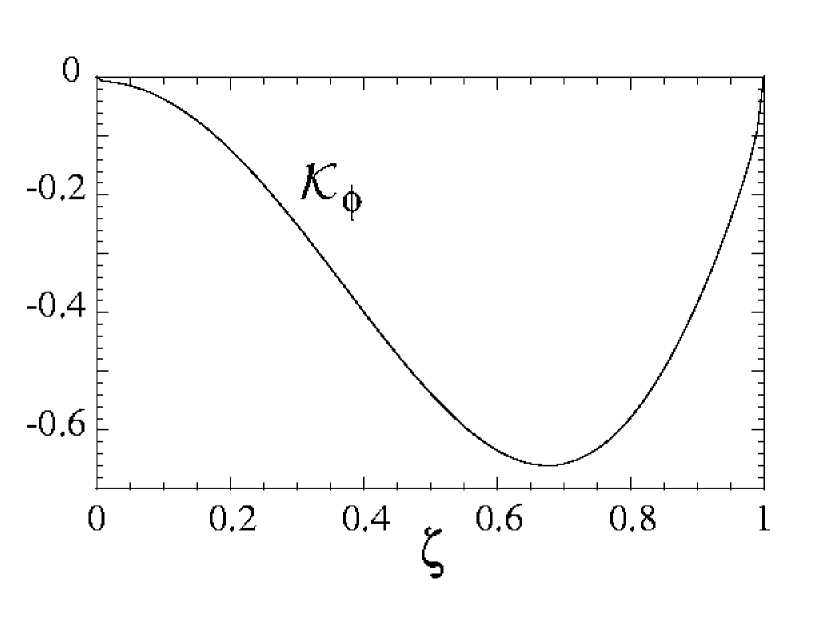
Figure 7.— The surface current density ${\cal K}_{\phi}$ is shown as a function of $\zeta=\cos(\theta)$, with $\theta$ is the colatitude, for the same case as Figure 6. The vertical scale is arbitrary.

6. Conclusions

An analytical model is developed for the screening of the external magnetic field of a rotating, magnetized, axisymmetric neutron star due to the accretion of plasma from a disk. The decrease of the field occurs due to the deposition of current carrying plasma onto the star’s surface. This plasma creates an induced magnetic moment with a sign opposite to that of the original magnetic dipole. The physical mechanism is explained in Figure 3. The equations (37) for the field evolution are inherently nonlinear and this leads to the generation of higher order modes when starting from the lowest order mode.

The main conclusions from this work are: (1) The field decreases independent of whether the star spins-up or spins-down (that is, for $r_{cr}>r_{A}$ or $r_{cr}<r_{A}$); (2) The time-scale for an appreciable decrease (by a factor $>100$) of the field is $t_{0}\sim 1.6\times 10^{7}$ yr for $\dot{M}=10^{-9}M_{\odot}$/yr and an initial stellar magnetic moment $\mu_{i}=10^{30}$ Gcm³ and it scales approximately as $\mu_{i}^{3.8}/\dot{M}^{1.9}$; (3) The decrease of the magnetic field does not have a simple relation to the accreted mass; (4) At late times the magnitude of the buried magnetic field is much larger than the initial field on the star’s surface; and (5) Once the accretion stops the field leaks out on an Ohmic diffusion time scale which is estimated to be $\gtrsim 10^{9}$ yr.

The present model has evident limitations which require further study: Accreting neutron stars are not expected to have their magnetic and rotational axes aligned. The case of small misalignment angles may be amenable to analytic treatment. The thickness of the accretion layer will in general be a function of position.

We thank Dr. Dong Lai for a number of valuable discussions. We also thank the referee for valuable recommendations. This work was supported in part by NASA grant NAG 5-13220 and NSF grant AST-0307817.

References

- (1)
- (2) Baym, G.H., Bethe, H.A., & Pethick, C.J. 1971, Nucl. Phys. A, 175, 225
- (3)
- (4) Bisnovatyi-Kogan, G.S., & Komberg, B.V. 1974, Astron. Zh., 51, 373 (1975,SvA, 18, 217)
- (5)
- (6) Cumming, A., Zweibel, E., & Bildsten, L. 2001, ApJ, 557, 958
- (7)
- (8) Cheng, K.S., & Zhang, C.M. 1998, A&A, 337, 441
- (9)
- (10) Cheng, K.S., & Zhang, C.M. 2000, A&A, 361, 1001
- (11)
- (12) Choudhuri, A.R., & Konar, S. 2002, MNRAS, 332, 933
- (13)
- (14) Gear, C.W. 1971, Numerical Initial Value Problems in Ordinary Differential Equations, ch. 9
- (15)
- (16) Ghosh, P., & Lamb, F.K. 1979, ApJ, 232, 259
- (17)
- (18) Gold, T., & Hoyle, F. 1960, MNRAS, 120, 7
- (19)
- (20) Goldreich, P., & Reisenegger, A. 1992, ApJ, 395, 250
- (21)
- (22) Hulse, R. A., & Taylor, J. H. 1975, AJ, 195, L51
- (23)
- (24) Illarionov, A.F., & Sunyaev, R.A. 1975, A&A, 39, 185
- (25)
- (26) Kato, S., Fukue, J., & Mineshige, S. 1998, Black-Hole Accretion Disks (Kyoto University Press: Kyoto, Japan), ch. 17
- (27)
- (28) Long, M., Romanova, M.M., & Lovelace, R.V.E. 2004, ApJ, submitted
- (29)
- (30) Lorimer, D. R. 2001, “Binary and Millisecond Pulsars at the New Millennium,” Living Reviews in Relativity, 4, 5; astro-ph/0104388
- (31)
- (32) Lovelace, R.V.E., Mehanian, C., Mobarry, C.M., & Sulkanen, M.E. 1986, ApJS, 62,1
- (33)
- (34) Lovelace, R.V.E., Romanova, M.M., & Bisnovatyi-Kogan, G.S. 1995, MNRAS, 275, 244
- (35)
- (36) Lovelace, R.V.E., Romanova, M.M., & Bisnovatyi-Kogan, G.S. 1999, ApJ, 514, 368
- (37)
- (38) Lynden-Bell, D.& Boily, C. 1994, MNRAS, 267, 146
- (39)
- (40) Lyne, A. G., Burgay, M., Kramer, M., Possenti, A., Manchester, R. N., Camilo, F., McLaughlin, M. A., Lorimer, D. R., D’Amico, N., Joshi, B. C., Reynolds, J., & Freire, P. C. C. 2004, Science, 303, 1153
- (41)
- (42) Payne, D.J.B., & Melatos, A. 2004, MNRAS, 351, 569
- (43)
- (44) Romani, R.W. 1990, Nature, 347, 741
- (45)
- (46) Romanova, M. M., Ustyugova, G. V., Koldoba, A. V., & Lovelace, R. V. E. 2002, ApJ, 578, 420
- (47)
- (48) Romanova, M. M., Ustyugova, G. V., Koldoba, A. V., & Lovelace, R. V. E. 2004, ApJ, 616, L151
- (49)
- (50) Ruderman, M. 1991, ApJ, 366, 261
- (51)
- (52) Shakura, N.I., & Sunyaev, R.A. 1973, A&A, 24, 337
- (53)
- (54) Trimble, V., Rees, M. 1970, The Crab Nebula, Proceedings from IAU Symposium No. 46, held at Jodrell Bank, England, August 5-7, eds. R. D. Davies and F. Graham-Smith (Dordrecht: Reidel). p.273
- (55)
- (56) van den Heuvel, E. P. J., & Bitzaraki, O. 1995, A&A, 297, L41
- (57)
- (58) Wijers, R.A.M.J. 1997, MNRAS, 287, 607
- (59)