Determining the Properties and Evolution of Red Galaxies from the Quasar Luminosity Function

Abstract

We examine the link between quasars and the red galaxy population using a model for the self-regulated growth of supermassive black holes in mergers involving gas-rich galaxies. In this picture, mergers drive nuclear inflows of gas, fueling starbursts and obscured quasars until feedback energy from black hole growth expels the surrounding gas, rendering the quasar briefly visible as a bright optical source. The quasar dies when there is no longer a significant supply of gas to power accretion, and the stellar remnant relaxes as a passively evolving spheroid satisfying the $M_{\rm BH}-\sigma$ relation and lying on the fundamental plane. The same process that halts black hole growth also terminates star formation in the remnant, accounting for the observed red galaxy population in the bimodal color/morphology distribution of galaxies. Using a model for quasar lifetimes and evolution motivated by hydrodynamical simulations of galaxy mergers, we de-convolve the observed quasar luminosity function at various redshifts to determine the birthrate of black holes of a given final mass. Identifying quasar activity with the formation of spheroids in the framework of the merger hypothesis, this enables us to infer the corresponding birthrate of spheroids with given properties as a function of redshift. With this method, we predict, for the red galaxy population, the distribution of galaxy velocity dispersions, the galaxy mass function, mass density, and star formation rates, the luminosity function in many observed wavebands (e.g., NUV, U, B, V, R, r, I, J, H, K), the total number density and luminosity density of red galaxies, the distribution of colors as a function of magnitude and velocity dispersion for several different wavebands, the distribution of mass to light ratios as a function of mass, the luminosity-size relations, and the typical ages and distribution of ages (formation redshifts) as a function of both mass and luminosity. For each, we predict the evolution at redshifts $z=0-6$ and, in each case, our results are in good agreement with observational estimates. However, we demonstrate that the predictions strongly disagree with observations if idealized, traditional models of quasar lifetimes are adopted in which these objects turn on and off at a fixed luminosity or follow simple exponential light curves, instead of the more complicated quasar evolution implied by our simulations.

1. Introduction

Hierarchical theories of galaxy formation and evolution indicate that large systems are built up over time through the merger of smaller progenitors. Galaxy interactions in the local Universe motivate the “merger hypothesis” (Toomre & Toomre 1972; Toomre 1977), according to which collisions between spiral galaxies produce the massive ellipticals observed at present times, a view supported by self-consistent modeling of mergers (for reviews, see e.g. Barnes & Hernquist 1992; Barnes 1998). Furthermore, it is believed that most galaxies harbor supermassive black holes (e.g. Kormendy & Richstone 1995; Richstone et al. 1998; Kormendy & Gebhardt 2001) and that the masses of these black holes correlate with either the mass (Magorrian et al. 1998) or the velocity dispersion (i.e. the $M_{\rm BH}$-$\sigma$ relation: Ferrarese & Merritt 2000; Gebhardt et al. 2000) of their host spheroids, demonstrating that the growth of supermassive black holes and galaxy formation are linked. Simulations of the self-regulated growth of black holes in galaxy mergers (Di Matteo et al. 2005) have shown that the energy released by this process can have a global impact on the structure of the remnant, implying that models of galaxy formation and evolution must account for black hole growth in a fully self-consistent manner.

Based on surveys such as SDSS, 2dFGRS, COMBO-17, and DEEP, there is mounting evidence that the color distribution of galaxies at $z=0$ is bimodal (e.g. Strateva et al., 2001; Blanton et al., 2003; Kauffmann et al., 2003a; Baldry et al., 2004; Balogh et al., 2004), and can be well fitted by two Gaussians (e.g. Baldry et al., 2004). The mean color and dispersion of these two (red and blue) distributions depend on luminosity, but little on galaxy environment (Blanton et al., 2003; Balogh et al., 2004; Hogg et al., 2004). This bimodality extends to moderate redshifts, $z\sim 1.5$ (e.g., Bell et al., 2003, 2004b; Willmer et al., 2005; Faber et al., 2005), and there exists a population of massive, very red galaxies at even higher redshift (e.g. Franx et al., 2003). The red galaxies in this bimodal distribution are almost all elliptical, absorption-line galaxies, at least at redshifts $z\lesssim 1$ (e.g., Strateva et al., 2001; Bernardi et al., 2003c; Bell et al., 2004a; Ball et al., 2005), which appear to be passively evolving from a redshift of peak star formation $z\sim 1.5-2.5$, according to both fundamental plane (e.g., van Dokkum et al., 2001; Treu et al., 2001, 2002; Gebhardt et al., 2003; Wuyts et al., 2004; van de Ven et al., 2003), and color and spectral analyses (e.g., Menanteau et al., 2001; Kuntschner et al., 2002; Treu et al., 2002; van de Ven et al., 2003; Bell et al., 2004b). It also appears that the properties of the red galaxies and their $z=0$ distribution, as well as their clustering and mass density evolution, are consistent with their being formed through mergers and thereafter relaxing quiescently (e.g., Kauffmann et al., 2003b; Budavári et al., 2003; Bell et al., 2003; Baldry et al., 2004; Weiner et al., 2005).

For mergers to produce red ellipticals from blue, star-forming disks and yield a bimodal color distribution, the color must evolve rapidly, or the observed bimodality would be washed out, requiring that star formation be terminated soon after a merger. Springel et al. (2005a) showed that this will not occur, especially in gas rich mergers at high redshift, if black hole feedback is neglected, because even a small amount of cold gas remaining after a powerful starburst will fuel a low level of star formation for a Hubble time (e.g. Mihos & Hernquist, 1994, 1996; Hernquist & Mihos, 1995), preventing the remnant from reddening sufficiently. However, Springel et al. (2005a) demonstrated that feedback from black hole growth and quasar activity caused by mergers can result in a much more violent and abrupt expulsion and heating of the remaining gas, as the black hole nears its final mass. This process also produces a remnant that satisfies observed correlations between black hole and host galaxy properties (Di Matteo et al., 2005).

Observations of elliptical galaxy ages and star formation histories motivate the notion of “anti-hierarchical” growth, or “cosmic downsizing,” (e.g., Bower et al., 1992; van Dokkum & Franx, 1996; Ellis et al., 1997; Bernardi et al., 1998; Jørgensen et al., 1996; Bell et al., 2004b; Faber et al., 2005), where the most massive spheroids are also the oldest and reddest systems. While black hole feedback is likely a key ingredient in shutting down star formation in these systems at high redshifts, allowing them to redden onto the observed $z=0$ color-magnitude relation, it does not automatically imply that particular black hole and galaxy formation scenarios are self-consistent. Moreover, although there is evidence of downsizing in quasar activity, with the most luminous quasars active at $z\sim 2$ and the peak formation redshift of quasars evolving as a function of luminosity (e.g. Page et al., 1997; Miyaji et al., 2000; Cowie et al., 2003; Ueda et al., 2003; Hasinger, Miyaji, & Schmidt, 2005; La Franca et al., 2005), it has not been demonstrated that the implied downsizing is consistent or even quantitatively similar to that of the galaxy population. As we demonstrate in what follows, the relationship between downsizing in galaxy and quasar populations depends sensitively on the model chosen for quasar light curves and lifetimes in any scenario in which spheroids and quasars form together.

In our picture, red, remnant spheroids and supermassive black holes are produced simultaneously in galaxy mergers which also yield starbursts and quasar activity. Previously, we studied black hole evolution in mergers using simulations (Hopkins et al. 2005a-e), and showed that the complex, luminosity-dependent quasar lifetimes and obscuration (Hopkins et al., 2005a, b) lead to a new interpretation of the quasar luminosity function (Hopkins et al., 2005c), where the faint end of the luminosity function consists mainly of quasars growing to much larger final masses or in declining states following peak quasar activity. This implies that the distribution of quasars being created at a given redshift as a function of the quasar peak luminosity or final black hole mass is peaked at a luminosity (mass) corresponding to the observed break in the luminosity function, falling off towards brighter and fainter luminosities. This differs from all previous models of quasar lifetimes, which predict that this distribution should have essentially identical shape to the observed luminosity function, increasing monotonically with decreasing luminosity (black hole mass). Because our simulations also yield observed correlations between black hole and remnant host galaxy properties, we can deduce the distribution and evolution of the remnant red galaxies produced in these merger events. These predictions will necessarily differ than those based on idealized models of quasar lifetimes, which yield a qualitatively different distribution of black hole masses (and thus host galaxy masses and velocity distributions) being formed at any given redshift.

Here, we use our models of quasar lifetimes and lightcurves and the observed quasar luminosity function to determine the rate at which quasars with a given peak luminosity or final black hole mass are born in mergers. Using the scaling relations between black hole and host galaxy properties derived from these simulations, we determine the birthrate of remnants with given properties as a function of redshift, and use this to predict the properties and evolution of the red, elliptical population in various wavebands. In § 2 we describe our methodology, including the simulations (§ 2.1), our model of quasar lifetimes and the quasar luminosity function (§ 2.2), and the black hole-host galaxy scaling relations obtained from the simulations (§ 2.3). In § 3 we use this information to predict the distribution of galaxy velocity dispersions with redshift, as well as the galaxy mass function and its evolution. In § 4 we obtain the galaxy luminosity function and its evolution in many observed wavebands and for redshifts $z=0-6$. In § 5 we predict the distribution of galaxy colors as a function of magnitude in several bands, velocity dispersion, and redshift. In § 6 we estimate the distribution of mass-to-light ratios and luminosity-size relation, and their differential evolution with time, as a function of mass and redshift. In § 7 we predict the distribution of formation ages (redshifts) as a function of galaxy mass, velocity dispersion, and luminosity. Finally in § 8 we discuss our results and their implications for observations and models of the joint formation of spheroids and active galactic nuclei (AGN).

Throughout, we adopt a $\Omega_{\rm M}=0.3$, $\Omega_{\Lambda}=0.7$, $H_{0}=70\,{\rm km\,s^{-1}\,Mpc^{-1}}$ cosmology. Unless otherwise stated, all magnitudes are in the Vega system.

2. Methodology

2.1. The Simulations

The simulations were performed using GADGET-2 (Springel, 2005), a new version of the parallel TreeSPH code GADGET (Springel, Yoshida, & White, 2001). GADGET-2 employs a fully conservative formulation (Springel & Hernquist, 2002) of smoothed particle hydrodynamics (SPH), which maintains simultaneous energy and entropy conservation even when smoothing lengths evolve (see e.g., Hernquist 1993b, O’Shea et al. 2005). Our simulations account for radiative cooling, heating by a UV background (as in Katz et al. 1996, Davé et al. 1999), and incorporate a sub-resolution model of a multiphase interstellar medium (ISM) to describe star formation and supernova feedback (Springel & Hernquist, 2003a). Feedback from supernovae is captured in this sub-resolution model through an effective equation of state for star-forming gas, enabling us to evolve disks with large gas fractions so that they are stable against fragmentation (see, e.g. Springel et al. 2005b; Springel & Hernquist 2005; Robertson et al. 2004, 2005a).

Supermassive black holes (BHs) are represented by “sink” particles that accrete gas at a rate $\dot{M}$ estimated from the local gas density and sound speed using an Eddington-limited prescription based on Bondi-Hoyle-Lyttleton accretion theory (Bondi 1952; Bondi & Hoyle 1944; Hoyle & Lyttleton 1939). The bolometric luminosity of the black hole is $L_{\rm bol}=\epsilon_{r}\dot{M}c^{2}$, where $\epsilon_{r}=0.1$ is the radiative efficiency. We assume that a small fraction (typical $\approx 5\%$) of $L_{\rm bol}$ couples dynamically to the surrounding gas, and that this feedback is injected into the gas as thermal energy. This fraction is a free parameter, which we determine as in Di Matteo et al. (2005) by matching the observed normalization of the $M_{\rm BH}-\sigma$ relation. For now, we do not resolve the small-scale dynamics of the gas directly around the black hole, but assume that the time-averaged accretion rate can be estimated on the scale of our spatial resolution (reaching $\approx 20$ pc, in the best cases).

The progenitor galaxies are constructed as described in Springel et al. (2005b). For each simulation, we generate two stable, isolated spiral galaxies, with dark matter halos having a Hernquist (1990) profile, motivated by cosmological simulations (e.g. Navarro et al. 1996; Busha et al. 2004), simple analytical arguments (e.g. Jaffe 1987; White 1987; see Barnes 1998, §7.3), and observations (e.g. Rines et al. 2002, 2002, 2003, 2004), an exponential disk of gas and stars, and (optionally) a bulge. The galaxies have masses $M_{\rm vir}=V_{\rm vir}^{3}/(10GH_{0})$ for $z=0$, with the baryonic disk having a mass fraction $m_{\rm d}=0.041$, the bulge (when present) has $m_{\rm b}=0.0136$, and the rest of the mass is in dark matter typically with a concentration parameter $9.0$. The disk scale-length is computed based on an assumed spin parameter $\lambda=0.033$, chosen to be near the mode in the observed $\lambda$ distribution (Vitvitska et al., 2002), and the scale-length of the bulge is set to $0.2$ times the resulting value.

Typically, each galaxy is initially composed of 168000 dark matter halo particles, 8000 bulge particles (when present), 24000 gas and 24000 stellar disk particles, and one BH particle. We vary the numerical resolution, with many of our simulations using instead twice as many particles in each galaxy, and a subset of simulations with up to 128 times as many particles. We vary the initial seed mass of the black hole to identify any systematic dependence of our results on this choice. In most cases, we choose the seed mass either in accord with the observed $M_{\rm BH}$-$\sigma$ relation or to be sufficiently small that its presence will not have an immediate effect. Given the particle numbers employed, the dark matter, gas, and star particles are all of roughly equal mass, and central cusps in the dark matter and bulge profiles are reasonably well resolved (see Fig 2. in Springel et al. 2005b).

The form of our fitted quasar lifetimes and galaxy scaling relations are based on a series of several hundred merger simulations, described in Robertson et al. (2005b) and Hopkins et al. (2005e). We vary the resolution, the orbital geometry, the masses and structural properties of the merging galaxies, the mass ratio of the galaxies, initial gas fractions, halo concentrations, the parameters describing star formation and feedback from supernovae and black hole growth, and initial black hole masses. The progenitors have virial velocities $V_{\rm vir}=80,113,160,226,320,{\rm and}\ 500\,{\rm km\,s^{-1}}$, constructed to resemble galaxies at redshifts $z=0,2,3,{\rm and}\ 6$, and span a range in final black hole mass $M_{\rm BH}\sim 10^{5}-10^{10}\,M_{\sun}$. This large set of runs allows us to investigate merger evolution for a wide range of galaxy properties and to identify any systematic dependence of our modeling. Moreover, the extensive range of conditions probed gives us a large dynamic range in our simulations, with final spheroid masses spanning $M_{\rm sph}\sim 10^{8}-10^{13}\,M_{\sun}$, covering nearly the entire observed range.

2.2. Quasar Lifetimes and the Quasar Luminosity Function

Previous theoretical studies of the quasar luminosity function have generally employed idealized quasar light curves, either some variant of a “feast or famine” or “light bulb” model (in which quasars have only two states: “on” or “off”, with constant luminosity in the “on” state; e.g., Small & Blandford, 1992; Kauffmann & Haehnelt, 2000; Haiman & Menou, 2000; Haiman, Quataert, & Bower, 2004) or a pure exponential light curve (constant Eddington-ratio growth or exponential decay; e.g., Haiman & Loeb, 1998; Volonteri et al., 2003; Wyithe & Loeb, 2003). However, our simulations of galaxy mergers suggest that these models are a poor approximation to the quasar lifetime at any given luminosity. The light curves from the simulations are complex, generally having periods of rapid accretion after “first passage” of the galaxies, followed by an extended quiescent period, then a transition to a peak, highly luminous quasar phase, and then a dimming as self-regulated mechanisms expel gas from the remnant center after the black hole reaches a critical mass. In addition, the accretion rate at any time can be variable over small timescales $\sim{\rm Myr}$, but despite these complexities, the statistical nature of the light curve can be described by simple forms, which we describe below.

From the simulations, we find that the differential quasar lifetime, i.e. the time spent by a quasar in a merger in a given logarithmic luminosity interval, is well fitted by an exponential,

$${\rm d}t/{\rm d}\log{L}=t^{\ast}_{Q}\,\exp[-L/L^{\ast}_{Q}],$$ (1)

where $L^{\ast}_{Q}$ is proportional to the peak quasar luminosity ($L_{\rm peak}$; roughly, the Eddington luminosity of the final black hole mass), and $t^{\ast}_{Q}$ is weakly dependent on peak luminosity. When quantified as a function of $L_{\rm peak}$ in this manner, the quasar lifetime shows no systematic dependence on any host galaxy properties, merger parameters, initial black hole masses, ISM and gas equations of state and star formation models, or any other varied parameters (Hopkins et al. 2005e).

If quasars of a given peak luminosity are being created or activated at a rate $\dot{n}(L_{\rm peak})$ at some redshift $z$, then, to first order in the quasar lifetime over the Hubble time, the observed quasar luminosity function (neglecting attenuation) is

$$\phi(L)\equiv\frac{{\rm d}\Phi}{{\rm d}\log L}(L)=\int{\frac{{\rm d}t(L,L_{\rm peak})}{{\rm d}\log(L)}\,\dot{n}(L_{\rm peak})}\,{\rm d}\log(L_{\rm peak}).$$ (2)

Knowing the quasar lifetime, we can invert this relation to determine the birthrate of quasars as a function of peak luminosity and redshift, $\dot{n}(L_{\rm peak})$. As shown in Hopkins et al. (2005e), the quasar luminosity functions in optical, UV, soft X-ray, and hard X-ray wavebands (including the effects of extinction) and at all measured redshifts are simultaneously well-fitted by a lognormal $\dot{n}(L_{\rm peak})$,

$$\dot{n}(L_{\rm peak})=\dot{n}_{\ast}\ \frac{1}{\sigma_{\ast}\sqrt{2\pi}}\exp\Bigl{[}-\frac{1}{2}\,\Bigl{(}\frac{\log(L_{\rm peak}/L_{\ast})}{\sigma_{\ast}}\Bigr{)}^{2}\Bigr{]}.$$ (3)

Here, $\dot{n}_{\ast}$ is the total number of quasars being created or activated per unit comoving volume per unit time; $L_{\ast}$ is the median of the lognormal, the characteristic peak luminosity of quasars activating (i.e. the peak luminosity at which $\dot{n}(L_{\rm peak})$ itself peaks), which is directly related to the break luminosity in the observed luminosity function (Hopkins et al., 2005c); and $\sigma_{\ast}$ is the width of the lognormal in $\dot{n}(L_{\rm peak})$, which determines the slope of the bright end of the luminosity function. The evolution of the quasar luminosity function with redshift is well-described by pure peak-luminosity evolution, where $\dot{n}_{\ast}$ and $\sigma_{\ast}$ are constant but $L_{\ast}=L_{\ast}^{0}\,\exp({k_{1}\,\tau})$. Here, $\tau$ is the fractional lookback time $\tau=H_{0}\,\int^{0}_{z}dt$. Above $z\sim 2-3$, the quasar population declines, but the detailed shape and evolution of the faint-end of the quasar luminosity function at these redshifts is poorly constrained from observations. Therefore we consider two choices: either pure peak-luminosity evolution (PPLE), where we multiply $L_{\ast}$ by a factor $\exp({-k_{2}\,[z-2]})$ for $z>2$, or pure density evolution (PDE), where we multiply the $z=2$ luminosity function by a normalization factor (i.e. multiply $\dot{n}_{\ast}$ by a factor) with identical functional form.

We follow Hopkins et al. (2005e), but fit to the more recent luminosity functions in the hard X-ray, soft X-ray, and optical from Ueda et al. (2003); Hasinger, Miyaji, & Schmidt (2005); Richards et al. (2005), respectively, and find the best-fit parameters $(\log(L_{\ast}^{0}/L_{\sun}),\,k_{1},\,k_{2},\,\log(\dot{n}_{\ast}/\ {\rm Mpc^{-3}\,Myr^{-1}}),\,\sigma_{\ast})=(11.3,\,4.0,\,0.65,\,-6.37,\,0.7)$. These are similar to the values given by Hopkins et al. (2005e) using older observations, although they suggest a somewhat narrower width in peak luminosities (with the peak more closely related to the break in the observed luminosity function).

From the form of the quasar light curve and lifetime as a function of luminosity, we can calculate the final black hole mass for a given $L_{\rm peak}$, and convert from $\dot{n}(L_{\rm peak})$ to $\dot{n}(M_{\rm BH})$, the birthrate of black holes of a given final (post-merger) mass. Accounting for the corrections owing to the non-trivial shape of the quasar light curve and lifetime, we obtain

$$M_{\rm BH}=M_{\rm Edd}(L_{\rm peak})\ [1.24\,(L_{\rm peak}/10^{13}\,L_{\sun})^{-0.11}].$$ (4)

Applying this conversion to our fitted $\dot{n}(L_{\rm peak})$, we find that $\dot{n}(M_{\rm BH})$ is also a lognormal, with identical redshift evolution and functional form, and $(\log(M_{\ast,\rm BH}^{0}/M_{\sun}),\,k_{1},\,k_{2},\,\log(\dot{n}_{\ast,\rm BH}/\ {\rm Mpc^{-3}\,Myr^{-1}}),\,\sigma_{\ast,\rm BH})=(6.45,\,3.2,\,0.59,\,-6.25,\,0.62)$.

Figure 1.— Predicted luminosity function (left, solid line) at $z=1$ using our model for quasar lifetimes and evolution. The corresponding hard X-ray luminosity function of Ueda et al. (2003) (circles) is shown for comparison, rescaled to bolometric luminosity following Hopkins et al. (2005e); Marconi et al. (2004); Vignali et al. (2003). The $\dot{n}(L_{\rm peak})$ distribution (rescaled in arbitrary units for comparison) is shown (dashed line), as is the $\dot{n}(L_{\rm peak})$ distribution obtained using a “light-bulb” or exponential light curve model of the quasar lifetime (dotted). On the right, the corresponding rate of formation of black holes/quasars of a given final mass, $\dot{n}(M_{\rm BH})$ is shown (dashed), as well as the rate of formation of remnant spheroids of a given virial (dotted; $\dot{n}(M_{\rm vir})$) and stellar (solid; $\dot{n}(M_{\rm sph})$) mass, determined from the $M_{\rm BH}-M_{\rm vir}$ and fundamental plane relations of our simulations (Robertson et al. 2005b).

Figure 1 shows an example of the results of our procedure for deconvolving an observed quasar luminosity function to obtain the black hole birthrate, using the Ueda et al. (2003) hard X-ray luminosity function at $z\sim 1$. The left panel gives the quasar luminosity function, where the black points are the observations and the line is the prediction from the quasar lifetimes and fitted $\dot{n}(M_{\rm BH})$ above. The right panel shows the corresponding $\dot{n}(M_{\rm BH})$ distribution at this redshift. The $\dot{n}(L_{\rm peak})$ [$\dot{n}(M_{\rm BH})$] distribution derived has the property that it peaks at a characteristic peak luminosity (black hole mass) corresponding to the break in the observed luminosity function, and falls off to both lower and higher luminosities. In this interpretation of the quasar luminosity function, “cosmic downsizing” follows naturally as the break in the quasar luminosity function moves to lower luminosities at lower redshifts, and the implied downsizing is indeed quantitatively more dramatic than that implied by idealized models of quasar activity (see § 6 and Figure 23 of Hopkins et al. 2005e).

It is important to note that the slope of the faint (low-$M_{\rm BH}$) end of $\dot{n}(M_{\rm BH})$ is only weakly constrained by the observed luminosity function, a point discussed further in § 4.1. To illustrate this, the figure shows the birthrate of quasars of a given peak luminosity, $\dot{n}(L_{\rm peak})$ (plotted in arbitrary units to demonstrate this qualitative behavior) as the dashed line. The $\dot{n}(L_{\rm peak})$ distribution which would be obtained using a “light-bulb” or exponential light curve model of the quasar lifetime is also shown (dotted line) for comparison (the $\dot{n}(M_{\rm BH})$, $\dot{n}(M_{\rm vir})$, $\dot{n}(M_{\rm sph})$ distributions for such a model will have the same shape as the $\dot{n}(L_{\rm peak})$ distribution, as explained below in § 2.3). The two models make very different predictions for luminosities/masses below those corresponding to the break in the observed luminosity function.

Although we do not consider the brief active quasar and starburst phases in our subsequent analysis (as they are heavily affected by rapidly evolving star formation, dust obscuration, merger dynamics, and quasar luminosities), we note that our modeling allows us to predict the behavior of the active quasar host galaxy luminosity function. We expect that the active quasars at a given redshift should have a narrow range in peak luminosities (black hole masses), corresponding to a narrow range in host galaxy stellar masses. This is shown in the $\dot{n}(L_{\rm peak})$ and $\dot{n}(M_{\rm sph})$ (derived below) distributions given in Figure 1. We therefore expect that the host galaxies of quasars active at a given time will have a much narrower range in luminosities than that predicted by e.g. idealized models of the quasar lifetime (for which $\dot{n}(L_{\rm peak})$ and therefore $\dot{n}(M_{\rm sph})$ must increase monotonically with decreasing luminosity/mass; see e.g. Lidz et al. 2005). There is observational support for this: the quasar host galaxy luminosity function is found to follow an approximately lognormal distribution with narrow width $\sigma_{\log(L,\,{\rm host})}\sim\sigma_{\log(M,\,{\rm host})}=0.2$ ($\sim 0.6-0.7$ magnitudes) and a peak roughly corresponding to the stellar mass of quasar hosts with $L_{peak}\sim$ the quasar luminosity function break luminosity (Bahcall et al., 1997; McLure et al., 1999; Hamilton et al., 2002).

2.3. Scaling Relations Among Galaxy and Black Hole Properties

Self-regulated black hole growth in our simulations yields a black hole mass-bulge velocity dispersion ($M_{\rm BH}-\sigma$) relation (Di Matteo et al., 2005) which agrees well with the observations of, e.g. Gebhardt et al. (2000); Ferrarese & Merritt (2000); Tremaine et al. (2002). Robertson et al. (2005b) further study this relation, and find it holds for mergers occurring at any redshift, with a constant slope and weak evolution in the normalization. From the simulations, they find

$$\log{(M_{\rm BH}/M_{\sun})}\approx 8.1+4.0\,\log\Bigl{(}\frac{\sigma}{200\,{\rm km\,s^{-1}}}\Bigr{)}-0.19\,\log(1+z).$$ (5)

The precise values depend on the fitting method, but in all cases agree well with those determined in Tremaine et al. (2002) for $z=0$. The scatter about this relation from the simulations is $\sim 0.3$ dex, similar to that observed. It is also important to note that the evolution seen in these simulations produces a $z=0$ scatter consistent with what is observed, which is not the case for all theoretical models (Robertson et al., 2005b).

The weak evolution in the $M_{\rm BH}-\sigma$ relation is caused by an increasing $\sigma$ for a given stellar mass with increasing redshift, as halos at higher redshift are more compact; the relation between black hole mass and total stellar mass ($M_{\rm BH}-M_{\rm sph}$) is independent of redshift. This independence is also suggested observationally by galaxy-AGN clustering properties as a function of redshift (Adelberger & Steidel, 2005). From our simulations, we can similarly determine the $M_{\rm BH}-M_{\rm vir}$ and $M_{\rm BH}-M_{\rm sph}$ relationship, giving

$$M_{\rm BH}=7.0\times 10^{-4}\,M_{\rm vir},$$ (6)

$$M_{\rm BH}=0.001\,M_{\rm sph},$$ (7)

in reasonable agreement with the observations of Marconi & Hunt (2003), if we account for the slightly different definitions of $M_{\rm vir}$ used. Here, $M_{\rm vir}$ is the virial mass within an effective radius, alternatively defined by $M_{\rm vir}=k\,\sigma^{2}R_{e}/G$, where to be definite we take $\sigma$ to be the average spheroid velocity dispersion within the effective radius $R_{e}$. For this conversion (where necessary) we adopt $k=5$, as is roughly seen in our simulations and expected for e.g. a Hernquist (1990) spheroid or $R^{1/4}$-law profile, and also similar to that suggested by comparison of mass measurements from dynamical modeling and from measurements of $\sigma$ and $R_{e}$ (e.g. Cappellari et al. 2005, although compare Marconi & Hunt 2003, who adopt $k=3$, which is the primary reason for the small discrepancy in the relation they observe and those we show above). The scatter about this relation from the simulations is small, about $\sim 0.3$ dex, similar to that observed.

We note that there are considerable observational contradictions regarding possible evolution in the $M_{\rm BH}-\sigma$ or $M_{\rm BH}-M_{\rm sph}$ relations, with e.g. Shields et al. (2003) and Adelberger & Steidel (2005) finding no evolution to $z\sim 3$ and e.g. Peng et al. (2005) and McLure et al. (2005) finding substantial evolution at $z<2$ (specifically, substantially undermassive bulges at $z\sim 2$). However, these observations are still difficult and have large uncertainties; furthermore, they specifically select primarily active, high Eddington ratio objects, which local observations (e.g., Barth et al., 2005) suggest may be biased to lie above the $M_{\rm BH}-\sigma$ relation in the manner observed. Above $z\sim 2$, the possibility for such evolution, and the uncertainty resulting from it, is essentially captured in our consideration of pure luminosity vs. pure density evolution for the quasar luminosity function, since these different evolutions imply a different peak luminosity (i.e. final spheroid mass) distribution. Thus, the uncertainties introduced by such evolution are not significantly larger than those we already describe, unless there is large evolution at $0<z<2$. Even such evolution in the $M_{\rm BH}-M_{\rm sph}$ relation will not change many of our conclusions, if the stellar mass of the final spheroid is primarily formed at this time, but is simply assembled (presumably in subsequent dry mergers) at later times. The alternative, that this stellar mass is formed between $z=2$ (when the massive black holes were formed) and $z=0$, is ruled out strongly by many observations which show the host spheroids of these black holes have old stellar populations with redshifts of formation $z\sim 1.5-2.5$ (e.g. Bower et al., 1992; Jørgensen et al., 1996; van Dokkum & Franx, 1996; Ellis et al., 1997; Bernardi et al., 1998; Jørgensen et al., 1999; van de Ven et al., 2003; Cross et al., 2004; Wuyts et al., 2004; Bell et al., 2004b; Förster Schreiber et al., 2004; Labbé et al., 2005).

Robertson et al. (2005c, in preparation) employ our simulations to study the fundamental plane relation between spheroid effective radius $R_{e}$, velocity dispersion $\sigma$, and stellar surface mass density $\Sigma$ of the merger remnants. In this, the projected stellar surface density $\Sigma$ is calculated along many different lines-of-sight, and for each, $R_{e}$ is determined as the two-dimensional radius enclosing half the stellar mass, and $\sigma$ is the mass-weighted line-of-sight stellar velocity dispersion within an aperture of radius $R_{e}$. When compared to e.g. the observed $K$-band fundamental place, for which a constant mass-to-light ratio is a reasonable approximation, the remnant spheroids of gas-rich mergers from our simulations fall on the observed infrared fundamental plane ($R_{e}\propto\sigma^{1.53}\Sigma^{-0.79}$, e.g., Pahre et al., 1998a, b) with little scatter. This relation and direct measurement yields a stellar mass-effective radius relation of the form $R_{e}\propto M_{\rm sph}(R_{e})^{\beta}$ (where $M_{\rm sph}(R_{e})$ is the stellar mass within the effective radius), or

$$\log(R_{e}/{\rm kpc})=\alpha+\beta\,\log(M_{\rm sph}(R_{e})/M_{\sun}).$$ (8)

The average $M_{\rm sph}(R_{e})-R_{e}$ relation found in our simulations has best-fit coefficients $\alpha=-5.81$, $\beta=0.57$, (i.e. $R_{e}\approx 0.86\,{\rm kpc}\,(M_{\rm sph}(R_{e})/10^{10}\,M_{\sun})^{0.57}$), in good agreement with observations (Shen et al., 2003) after accounting for the small difference between effective radius used here and half-light radius observed. The exact relation has a weak dependence on redshift, which we include; but we find little difference in our results in either case as, for example, at $z=0$, $\alpha=-5.6,\ \beta=0.56$, and at $z=2$, $\alpha=-5.4,\ \beta=0.53$. Observations also suggest only weak evolution in this relation (e.g. Trujillo & Aguerri, 2004; Trujillo et al., 2004, 2005; McIntosh et al., 2005b).

We use this relation to convert between mass-to-light ratios as a function of stellar mass to a luminosity-size relation in § 6, but we can also use it to determine the spheroid stellar mass as a function of virial (dynamical) mass and black hole mass. Combining the equations above,

$$\frac{M_{\rm sph}(R_{e})}{M_{\rm vir}}\approx 0.3\,\Bigl{(}\frac{M_{\rm vir}}{10^{10}\,M_{\sun}}\Bigr{)}^{-0.2}.$$ (9)

This agrees well with observations (e.g. Bernardi et al. 2003a, Padmanabhan et al. 2004; Cappellari et al. 2005) and additionally follows from the observed $M_{\rm sph}-R_{e}$ relation given that $M_{\rm BH}\propto\sigma^{4}\propto M_{\rm vir}$. Note that we have defined the stellar mass $M_{\rm sph}(R_{e})$ as that within the effective radius $R_{e}$; this means that the total galaxy stellar mass is $M_{\rm sph}\approx 2\,M_{\rm sph}(R_{e})$. These relations are determined from the simulations to be independent of redshift (except for the weak evolution in $M_{\rm sph}-R_{e}$ which we account for). When only the total stellar mass is needed, we use the directly fitted $M_{\rm BH}-M_{\rm sph}$ relation described above as it both avoids the uncertainties inherent in these conversions and accounts for e.g. changing bulge-to-disk ratios as a function of mass.

In what follows, we are not concerned with the structure of individual galaxies, and so defer a detailed structural analysis of merger remnants (Robertson et al. 2005c, in preparation). We instead use the relations above to study the statistical properties (i.e. conditional age and mass distributions) and evolution of the red galaxy population. We emphasize that although we use the form of these relations from our simulations, because each agrees well with its observed counterpart, it makes no difference to our results whether we use the relations from our simulations or adopt the observed scalings.

The simulations yield relationships between black hole mass and either velocity dispersion or stellar spheroid mass that can be used to transform the birthrate of black holes of a given final mass $M_{\rm BH}$, $\dot{n}(M_{\rm BH})$ into a birthrate of remnants with definite velocity dispersion $\dot{n}(\sigma)$ or stellar spheroid mass $\dot{n}(M_{\rm sph})$. This is illustrated in Figure 1, where the right panel gives the $\dot{n}(M_{\rm vir})$ (dotted) and $\dot{n}(M_{\rm sph})$ (solid) relations derived using the fitted relations above, our modeling of quasar lifetimes, and the observed quasar luminosity function. Although there are several steps in this procedure, we emphasize that all of the relationships used, each agreeing with observations, are determined entirely from the simulations alone, in a self-consistent manner. Any additional modeling required beyond this point is further calculated self-consistently from the simulations and is directly constrained by observations of quasars (e.g. the cases of obscuration and quasar lifetimes; Hopkins et al. 2005e) or galaxies (e.g. star formation and stellar population synthesis models; Bruzual & Charlot 2003). The lone observational input is the observed quasar luminosity function, from which we derive the birthrate of spheroids of a given mass (or velocity dispersion).

In our simulations, merger remnants resemble elliptical galaxies, with small gas fractions, and star formation is terminated by feedback as the black hole reaches its final mass. Thereafter, the galaxies mainly evolve passively, without significant star formation. The timescale for the merger-induced starburst is $\sim 100$ Myr (e.g. Springel et al. 2005a), much shorter than the merger timescale $\sim$Gyr. We therefore adopt the approximation that the merger occurs instantly at the redshift being considered, and that the remnant does not evolve after that point (at least to very high redshifts where the Hubble time becomes comparable to the timescale for the merger). We have actually considered two cases: one where we assume each spheroid is formed instantly at the redshift under consideration, and a second where we assume the starburst to have a Gaussian shape in time with a peak at $z$ and characteristic falloff timescale (standard deviation) $\sim 100$ Myr. We find essentially no difference in our predictions between these cases, except for a slight reddening of typical galaxy colors at high redshift in the latter case. We also do explicitly calculate the possible consequences of subsequent “dry merging” in § 4.1 below, and show that they are small.

Given the birthrate of spheroids, we use the stellar population synthesis models of Bruzual & Charlot (2003) to determine their observed luminosities and colors. The remnants in our simulations typically have solar metallicities, even at high redshift, (as expected from observations of high-redshift red galaxies, e.g. van Dokkum et al., 2004; Förster Schreiber et al., 2004) as metal enrichment occurs through star formation and associated supernova feedback in the most dense regions of the galaxy and metals are distributed throughout the galaxy by quasar feedback (Cox et al., 2005a). To examine the impact of the metallicity on the stellar population, we consider two cases: one in which the remnants are assumed to have solar metallicity ($0.02$) and the second where they have a Gaussian metallicity distribution (with a mean solar metallicity) and standard deviation $\sim 0.005-0.01$. We find little difference in our results between these two cases.

A scaling of metallicity with mass or velocity dispersion $\sigma$ could also influence our predicted luminosity functions. There is some observational evidence of a correlation between metallicity and $\sigma$ (e.g. Worthey et al., 1992; Jørgensen, 1997; Kuntschner, 2000), but the inferred metallicities are degenerate with the modeled population ages (Worthey et al., 1995; Faber et al., 1995; Worthey, 1997) and some studies infer no connection between metallicity and either velocity dispersion or age (e.g. Bernardi et al., 2003c, 2005) or find that the observed scaling of Mg and H$\beta$ line profiles is consistent with more massive ellipticals having formed earlier (e.g. Fisher et al., 1995, 1996). Moreover, the analysis of the joint correlation of metallicity with age and velocity dispersion of Jørgensen (1999); Jørgensen et al. (1999) indicates that the relation between typical age and $\sigma$ implies very little net change in metallicity in observed populations. Also, it is the Mg₂ and H$\beta$ line indices which are well-correlated with velocity dispersion (Burstein et al., 1988; Worthey et al., 1992; Blakeslee et al., 2001); the $\left<{\rm Fe}\right>$ index shows only weak correlation with velocity dispersion (Jørgensen, 1997; Trager et al., 1998) and so it is not clear whether this is a result of an enhancement of $\alpha$ elements or depressed Fe, and therefore it is difficult to translate to metallicity. Regardless of these uncertainties, the effect is considerably smaller than that of changing mean spheroid ages with mass (as demonstrated in § 6 and § 7 below), as e.g. even for the extreme case of the evolution reported by Kuntschner (2000), with $[{\rm Fe/H}]=0.56\,\log(\sigma/100\,{\rm km\,s^{-1}})$, this results in only a change from $Z\sim 0.8\,Z_{\sun}$ at $M_{\rm sph}\sim 5\times 10^{7}\,M_{\sun}$ to $Z\sim 2.2\,Z_{\sun}$ at $M_{\rm sph}\sim 2\times 10^{9}\,M_{\sun}$, ultimately shifting e.g. the $z=0$ B-band galaxy luminosity function by only $\sim 0.1$ magnitude.

Because these effects are weak compared to the age effects in the stellar populations we model, we do not impose a scaling of metallicity with mass or velocity dispersion, deferring a treatment of the chemical enrichment histories of galaxies to future work (but see, e.g. Brook et al., 2004a, b; Robertson et al., 2005d; Font et al., 2005), but note that its addition does not create any conflict between our predictions and observations. However, these relatively small scalings could be important for the observed colors, so we do briefly consider the possible effects of changing metallicity with $\sigma$ in § 5, where we show that the effect is small. We do not include the effects of dust reddening on the galaxy population, as our simulations show a dramatic and rapid falloff in characteristic column densities after the starburst, when the black hole expels surrounding gas as it reaches its final mass. This is consistent also with observations that show that only a small fraction $\lesssim 10\%$ of the luminosity in red galaxies can come from dusty, intrinsically bluer sources (Bell et al., 2004a).

3. The Relic Velocity Dispersion Distribution and Mass Functions

In § 2.1 and § 2.3 we have determined $\dot{n}(M_{\rm BH})$, the rate at which quasars of a given final black hole mass are formed in mergers, and fit this to an analytical form. Having also determined the $M_{\rm BH}-\sigma$ relation as a function of redshift and its intrinsic dispersion from our simulations, we can then convert $\dot{n}(M_{\rm BH})$ to $\dot{n}(\sigma)$, the birthrate of spheroids of a given velocity dispersion as a function of redshift. To do so, we account for the intrinsic dispersion of the $M_{\rm BH}-\sigma$ relation, by inverting

$$\dot{n}(M_{\rm BH})=\int^{\infty}_{0}P(M_{\rm BH}|\sigma)\ \dot{n}(\sigma)\,{\rm d}\sigma,$$ (10)

where we assume that $P(M_{\rm BH}|\sigma)$ is distributed as a lognormal about the value given by the $M_{\rm BH}-\sigma$ relation, with a dispersion equal to that in our determined (and the observed) relation, $\sim 0.3$ dex. With our modeling of spheroid and black hole co-formation in a single (dominant) major merger, the inversion of Equation 10 above is straightforward, as derived by Yu & Lu (2004) as a method to determine the velocity distribution function at various redshifts for which direct observations of velocity dispersions are inaccessible. Thus, knowing $\dot{n}(\sigma)$, we can integrate over time (redshift) to determine the relic number density of sources with a given velocity dispersion, $n(\sigma)={\rm d}n/{\rm d}\log(\sigma)$.

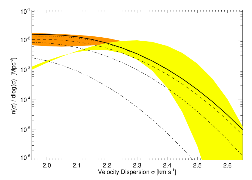
Figure 2.— The relic distribution of velocity dispersions (as defined in § 2.3 and as would be inferred from the $M_{\rm BH}-\sigma$ relation) at $z=0$ (solid), 1 (dotted), 2 (dashed), 3 (dot-dashed), and 5 (triple-dot-dashed). The $1\sigma$ range of observations of velocity dispersions in elliptical galaxies is shown, from Sheth et al. (2003) (yellow shaded region), with the contribution from bulges in S0 and spiral galaxies from Aller & Richstone (2002) (orange shaded region).

The results of this integration to $z=0$ are shown in Figure 2 (thick solid line). Our theoretical estimate agrees well with the observed distribution of velocity dispersions found for local $z=0$ ellipticals by Sheth et al. (2003) ($1\sigma$ range shown as the yellow shaded region). The contribution from spheroids in S0 and spiral galaxies, determined by Aller & Richstone (2002), is added to this and shown also at the low-$\sigma$ end where it dominates ($1\sigma$ range shown as orange shaded region). We caution that our prediction at low-$\sigma$ is somewhat sensitive to the assumed faint-end slope in the birthrate of black holes of a given mass [$\dot{n}(M_{\rm BH})$], as these are not necessarily the products of major mergers. Our estimate is on the high side at the extreme large-$\sigma$ tail of the distribution, but this is where both the observations are uncertain and our modeling of the quasar luminosity function and corresponding black hole mass [$\dot{n}(M_{\rm BH})$] distribution are sensitive to the functional form and bolometric corrections adopted.

We can also predict the velocity dispersion function at different redshifts based on our modeling, and these results are shown in Figure 2. We note that we have adopted the pure-peak luminosity evolution (PPLE) form for the evolution of the quasar luminosity function above $z\sim 2$, where the break and faint-end slope of the luminosity function are poorly constrained. If we instead consider the pure density form of this evolution, the $z=3$ and $z=5$ distributions peak at significantly higher $\sigma$.

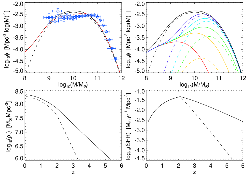
Figure 3.— Predicted $z=0$ stellar mass function in remnant red, elliptical galaxies (upper left). This is compared to the morphologically selected spheroid stellar mass function of Bell et al. (2003) (blue diamonds, where horizontal errors show the systematic mass uncertainty). Red dot-dashed line shows our prediction allowing for subsequent dry mergers. Upper right shows the mass function at $z=0$ (black), $z=0.5$ (blue), $z=1$ (cyan), $z=2$ (green), $z=2$ (orange), and $z=5$ (red). Lower left shows the integrated stellar mass density as a function of redshift, lower right the star formation rate. The solid lines adopt pure peak luminosity evolution for the quasar luminosity function above $z=2$, the dashed lines adopt pure density evolution.

We can perform an identical procedure, using instead the relations between black hole mass and host galaxy stellar mass to obtain the relic stellar mass function and its evolution with redshift. Figure 3 shows the resulting $z=0$ stellar mass function in remnant red, elliptical galaxies (upper left). This is compared to the morphologically selected spheroid stellar mass function of Bell et al. (2003) (blue diamonds, where horizontal errors show the systematic mass uncertainty). In all panels, the solid lines adopt pure peak luminosity evolution (PPLE) for the quasar luminosity function above $z=2$, and the dashed lines are for pure density evolution (PDE), as defined in § 2.2. The agreement is good over the entire range of observed masses, especially considering the systematic uncertainties in the observations. As is demonstrated for the galaxy luminosity function in Figure 4, adopting an idealized “light-bulb” or pure exponential light curve model for the quasar lifetime will not produce the turnover and shallow slope of the faint end of this mass function, and will overpredict the low-mass end by $2-3$ orders of magnitude. The upper right of the figure shows the mass function at various redshifts, the lower left shows the integrated stellar mass density as a function of redshift, and the lower right the star formation rate. The evolution of the star formation rate qualitatively agrees well with that estimated by, e.g. Cole et al. (2001), but we do not account for the star-forming spiral population which constitutes a significant or even dominant fraction of the integrated star formation rate, and so our present results are not necessarily in conflict with cosmological simulations indicating that the total mean density of cosmic star formation peaks at $z\approx 4-5$ (see, e.g. Springel & Hernquist 2003b; Hernquist & Springel 2003; Nagamine et al. 2004a).

Subsequent gas-poor (“dry”) mergers, by definition, do not have a reservoir of cold gas, and as a result cannot excite bright quasar activity. Therefore, the empirical information we derive on the rate at which spheroids are born as a function of mass and redshift from the quasar luminosity function does not account for dry merging. However, we can estimate the potential impact of spheroid-spheroid mergers on our predictions. Recent observations (Bell et al., 2005; van Dokkum, 2005) suggest that $z=0$ spheroids have, on average, undergone $\sim 0.5-1$ major dry mergers since $z\sim 0.7$ (see also Carlberg et al. 1994; Le Fèvre et al. 2000; Patton et al. 2002; Conselice et al. 2003, although de Propris et al. 2005 estimate a significantly lower value $\sim 0.2$). Observations and our predictions for the birth redshifts of spheroids (see § 7) imply that there should not be significant dry merging much earlier, as most spheroids are either recently formed or still forming at higher redshifts. Therefore, we can estimate the effects of dry merging by assuming that each spheroid has undergone $\sim 0.5$ major dry mergers in its history down to $z=0$. For simplicity, we assume these are equal-mass dry mergers; i.e. for a given interval in mass, we assume half the number of predicted spheroids dry merge, halving their number density but doubling their mass.

The resulting mass function is shown by the red dot-dashed line in the upper left of Figure 3 (for the pure peak luminosity evolution case). The net resulting change, as dry merging increases spheroid masses but decreases the total number of spheroids, is generally smaller than typical uncertainties in our modeling (of, e.g. the functional form of $\dot{n}(M_{\rm BH})$) and the observations, and thus we can safely ignore the impact of dry merging in our subsequent analysis. This is also suggested by calculation of e.g. the spheroid luminosity function from semi-analytical models (Cirasuolo et al., 2005). The effect is not completely negligible, however, and we note that the dry-merging corrected mass function agrees very well with the observations (within $\sim 1\sigma$ at all masses). Because dry mergers are not constrained by our empirical approach (unlike gas-rich mergers which produce a signal in the quasar luminosity function), and the rate and impact of dry galaxy mergers is observationally uncertain, we do not include their effects in any of our other predictions, but emphasize here that they introduce a relatively small second-order effect which does not result in any conflict with the observations.

4. Galaxy Luminosity Functions

4.1. The B-band Luminosity Function at All Redshifts

Unlike the relic velocity dispersion function, which is determined by the integrated history of spheroids, the evolution of stellar luminosities and colors makes the galaxy luminosity function in different wavebands dependent on the time history of spheroid formation. Because of this, it is not implicit that successfully reproducing the $z=0$ black hole mass distribution will guarantee an accurate prediction for the galaxy luminosity function at $z=0$ or higher redshifts.

As outlined in § 2.3, we use the observed quasar luminosity function and our simulations of quasar evolution to determine the birthrate of black holes of mass $M_{\rm BH}$, and correspondingly spheroids of stellar mass $M_{\rm sph}$, as a function of redshift. For a given observed redshift $z_{\rm obs}$, we can then integrate over $z>z_{\rm obs}$ to determine the history of the spheroids observed at $z_{\rm obs}$; i.e. for a given $z_{\rm obs}$ and $M_{\rm sph}$, the distribution of ages/formation times is completely determined. Knowing the formation history for these spheroids, we use the stellar population synthesis model of Bruzual & Charlot (2003) to determine their observed magnitudes in any given band at $z_{\rm obs}$.

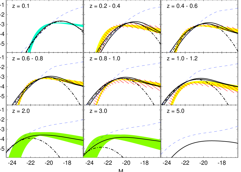
Figure 4.— Predicted B-band red/elliptical galaxy luminosity function (solid lines) at different redshifts (shown in the upper left of each panel). For panels with a range of redshifts shown, the lines show our prediction at the minimum and maximum redshift. Dot-dash lines show the prediction assuming pure density evolution instead of pure peak luminosity evolution above $z\sim 2$, at the mean redshift of each bin. Shaded ranges show the $1\sigma$ range of observed luminosity functions from Madgwick et al. (2002, cyan), Faber et al. (2005, yellow and red), Giallongo et al. (2005, green). The blue dashed line shows the prediction obtained used an idealized model for the quasar lifetime in which quasars grow/decay exponentially or turn on/off as a step function.

We show our prediction for the rest-frame B-band red/elliptical galaxy luminosity function at a series of observed redshifts in Figure 4. In each panel, our predicted B-band luminosity function for the redshift indicated in the upper left is shown as the thick black line. When a range of $z$ is indicated in the upper left of a panel, the predicted luminosity functions at both the minimum and maximum redshift of the range are given. The $1\sigma$ range in the observed luminosity function at each redshift (or redshift range) is indicated as a shaded region. At $z\sim 0-0.1$ (median $z=0.04$), the observed luminosity function of Madgwick et al. (2002), determined from the 2dFGRS survey, is shown in cyan. At $z=0.2-0.4,\ 0.4-0.6,\ 0.6-0.8,\ 0.8-1.0,\ {\rm and}\ 1.0-1.2$, the shaded region shows the observed luminosity functions from Faber et al. (2005), determined from the DEEP2 (yellow) and COMBO-17 (red) surveys (Bell et al., 2004b; Willmer et al., 2005). At $z=2.0$ and $z=3.0$, the observations from Giallongo et al. (2005), from the Hubble Deep Field and K20 surveys, are shown in green. At $z=5$ there is no observed B-band luminosity function, but we show our prediction.

In each case, the observed luminosity function is determined from either morphologically-selected elliptical galaxies or color-selected red galaxies (especially at high redshift where morphological information is not available), which as noted in § 1 are similar at least at low to moderate $z\lesssim 1-2$ redshifts (e.g. Strateva et al., 2001; Bernardi et al., 2003c; Bell et al., 2004a; Ball et al., 2005). Our predictions agree well with the observations, over a wide range of magnitudes and redshifts. We slightly overpredict the bright end of the luminosity function at high redshift, but this can be explained by selection effects, as we show below in § 5, because many of these very bright, high-redshift galaxies are quite blue (as they have formed only recently at these high redshifts) and thus would not appear in an observed red galaxy luminosity function (although this is also somewhat related to our slight overprediction of the high-$\sigma$ end of the velocity dispersion function in Figure 2).

In Figure 4, we also show the predicted B-band red/elliptical galaxy luminosity function at each redshift using a commonly employed, idealized model for the quasar lifetime (blue dashed lines). Here, we assume that a quasar radiates at its peak luminosity $L=L_{\rm peak}$ for a fixed time equal to $10^{7}$ yr (as is often adopted, and similar to the Salpeter time for $e$-folding of an Eddington-limited black hole, $t_{S}=4.2\times 10^{7}$ yr), but we note that the entire class of “light-bulb” or exponential growth/decay models for the quasar light curve produces a nearly identical prediction to that shown. This model overpredicts the number of red/elliptical galaxies which should be observed at low luminosities by two orders of magnitude, does not reproduce the shape and curvature of the luminosity function, and underpredicts the bright end if the lifetime is chosen to be longer (e.g. the actual Salpeter time). The quasar lifetime in these models is a free parameter, but it determines only the normalization of this curve, and thus no value can produce a reasonable prediction for the galaxy luminosity function. The reason for the failure of these models at low luminosity is, as mentioned above, the fact that they associate objects observed at low luminosities with low-$L_{\rm peak}$ objects, and therefore low-$M_{\rm BH}$ objects in small-mass spheroids.

Figure 4 also shows our prediction (dot-dashed lines), for the mean redshift of each bin, assuming pure density evolution (PDE) instead of pure peak luminosity evolution (PPLE) for the birthrate of quasars with a given peak luminosity above $z\sim 2$. Although the observed quasar luminosity function does not provide a good constraint on which evolution is followed, the difference in our subsequent calculations is usually minimal, and observations of the faint end of the galaxy luminosity function at moderate and high redshifts (where the two predictions begin to diverge) do not yet exist. However, if such observations of the galaxy population can be made, or the ages of the lowest-mass/luminosity objects at $z\sim 0$ are measured, they can provide a powerful constraint on the $\dot{n}(L_{\rm peak})$ [$\dot{n}(M_{\rm BH})$, $\dot{n}(M_{\rm sph})$] distributions (i.e. the rates at which spheroids and quasars of given properties form with redshift).

4.2. The Evolution of the Luminosity Function with Redshift

The observed galaxy luminosity function is usually fit to a Schechter function (Schechter, 1976) with normalization $\phi^{\ast}$, characteristic magnitude (luminosity) $M^{\ast}$ ($L^{\ast}$), and faint-end slope, $\alpha$. This yields a total number density of galaxies $\Phi=\phi^{\ast}\,\Gamma(\alpha+1)$, and a total luminosity density $j=\phi^{\ast}\,L^{\ast}\,\Gamma(\alpha+2)$. We can determine $\Phi$ and $j$ by integrating our predicted luminosity function at each redshift. However, observationally, it is easier to determine $\phi^{\ast}$ than $\Phi$, as $\alpha$ is difficult to measure and a constant $\alpha$ is often assumed. To compare directly with most observations (e.g., Cohen, 2002; Bell et al., 2003; Madgwick et al., 2003; Giallongo et al., 2005; Faber et al., 2005), we therefore assume a constant $\alpha_{0}=0.5$ and calculate $\phi^{\ast}\equiv\Phi/\Gamma(\alpha_{0}+1)$ and likewise calculate $M^{\ast}$ [$L^{\ast}\equiv j/(\phi^{\ast}\,\Gamma(\alpha_{0}+2))$].

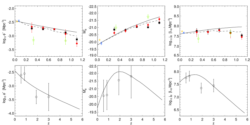
Figure 5.— B-band luminosity function normalization $\phi^{\ast}$ (left), characteristic magnitude $M^{\ast}_{B}$ (center), and luminosity density $j_{B}$ (right) predicted by our model (black lines) as a function of redshift for $z=0-6$. Upper panels show the $z\lesssim 1$ range in greater detail. Dashed lines show the prediction ignoring recent ($<1$ Gyr) mergers. Observations are from Faber et al. (2005) (COMBO-17, red circles, and DEEP2, black squares), Madgwick et al. (2003) (2dF, orange diamonds), Bell et al. (2003) (SDSS, blue $\times$’s), and Im et al. (2002) (DEEP1, green stars) for the low-redshift (upper) panels. Results from Giallongo et al. (2005) (Hubble Deep Field and K20, open black circles) at high redshift (lower panels) are also shown.

Figure 5 shows $\phi^{\ast}$, $M^{\ast}_{B}$, and $j_{B}$ as a function of redshift. Our prediction is shown as a solid black line both in a low redshift interval $z<1.2$ (upper panels) and over the entire $z<6$ interval (lower panels). At low redshifts (upper panels), observations from Faber et al. (2005) (COMBO-17, red circles, and DEEP2, black squares), Madgwick et al. (2003) (2dF, orange diamonds), Bell et al. (2003) (SDSS, blue $\times$’s), and Im et al. (2002) (DEEP1, green stars) are shown, with $1\sigma$ errors, and at high redshifts (lower panels), observations from Giallongo et al. (2005) (Hubble Deep Field and K20) are shown (circles).

Although we slightly overpredict $\phi^{\ast}$ (and thus $j_{B}$ as a consequence) at $z\sim 1.2$, this is related directly to our small overprediction of the bright blue end of the luminosity function discussed in § 4.1 and, as discussed in § 5 can be explained by selection effects as these objects have recently formed and are bluer than their traditionally color-selected counterparts. We estimate the results of this selection effect in the upper panels, where the dashed lines show our prediction ignoring all objects which have formed (i.e. gone through their peak merger/quasar activity) less then 1 Gyr in the past, and thus have not had sufficient time to redden to the point where they would be recognized as red galaxies in color-selected surveys (this corresponds roughly to the color selection of e.g. Bell et al. 2004b, given our modeled metallicities and star formation histories). The agreement at $z\sim 1-1.2$ is significantly improved, suggesting that the strong increase in red galaxies from $z\sim 1$ to present is driven in part by continued formation and mergers associated with ongoing (though declining) quasar activity, and in part by the reddening of spheroids formed in mergers at the peak of quasar activity $z\sim 1-2$, reddening to the point where they will be recognized as red ellipticals by $z\sim 0$.

Because, in our picture, spheroids and quasars form together through mergers, the quantities $\phi^{\ast}$, $M^{\ast}_{B}$, and $j_{B}$ are directly related to the quasar luminosity function. Associating each merger with a single quasar and spheroid, the total number of red galaxies is given by the integrated number of quasars produced up to the observed redshift; i.e. $\Phi=\int_{\infty}^{z_{\rm obs}}\dot{n}(QSO)\,dt$, where $\dot{n}(QSO)$ is the number density of quasars born per unit time per unit comoving volume. In our determination of the luminosity function, this is $\dot{n}_{\ast}=\,$constant, the normalization of the lognormal $\dot{n}(M_{\rm BH})$ distribution. Thus $\phi^{\ast}=\dot{n}_{\ast}t_{H}(z)/\Gamma{(\alpha+1)}$, where $t_{H}$ is the age of the Universe at a particular redshift. Note that if we adopted pure density evolution for the quasar luminosity function above $z\sim 2$, $\dot{n}_{\ast}$ would fall off exponentially above these redshifts, and $\phi^{\ast}$ would drop correspondingly. Currently, the observations are insufficient to decide which possibility is correct, but this makes it clear that estimating the total number of red galaxies at high redshift in future observations can constrain the form of the quasar luminosity function evolution.

Likewise, $M^{\ast}$ is directly related to the break in the observed quasar luminosity function, which in turn corresponds directly to the peak in the $\dot{n}(L_{\rm peak})$ [and corresponding $\dot{n}(M_{\rm BH})$] distribution (Hopkins et al., 2005c), and thus gives the peak in the rate at which spheroids of a given stellar mass are forming as a function of that stellar mass. Because luminosities evolve with the age of the stellar population, this is not trivially related to the $M^{\ast}$ of the galaxy population as $\Phi$ is to the number density of quasars being formed, but the two are still critically related and, in general, increasing $M^{\ast}$ corresponds to moving the break in the observed quasar luminosity function to higher luminosities, and vice versa.

4.3. The Luminosity Function in Different Wavebands

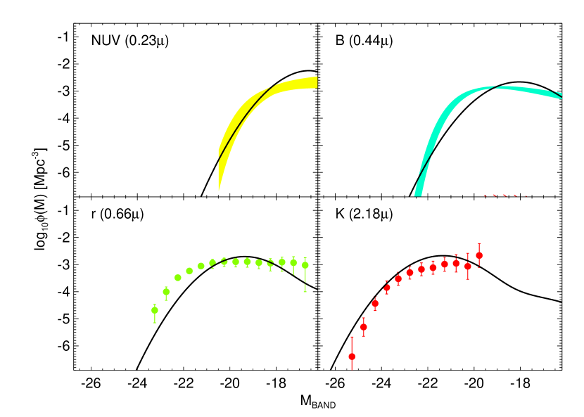
Figure 6.— Predicted $z\sim 0$ red/elliptical galaxy luminosity function in four wavelengths (black lines), in the manner of Figure 4. Observations are from Budavári et al. (2005); Treyer et al. (2005) in the near UV (NUV; yellow; upper left), Madgwick et al. (2002) in B-band (cyan; upper right), Nakamura et al. (2003) in Sloan $r$-band (green; lower left), and Kochanek et al. (2001) in K-band (red; lower right).

Figure 6 shows our predicted red/elliptical galaxy luminosity function (solid lines) in several different wavebands at $z\sim 0$; the near ultraviolet (NUV; at $2400$ Å or $0.24\,\mu$), B-band ($0.44\,\mu$), r-band ($0.66\,\mu$), and K-band ($2.18\,\mu$). Each is compared to the observations (shaded regions or points showing $1\sigma$ errors), shown over the range of magnitudes where data exist. The observations shown are from Budavári et al. (2005) and Treyer et al. (2005) in the NUV from GALEX (yellow; upper left), Madgwick et al. (2002) in B-band from 2dFGRS (cyan; upper right), Baldry et al. (2004) (see also Nakamura et al. 2003) in Sloan $r$-band from SDSS (green; lower left), and Kochanek et al. (2001) in K-band from 2MASS (red; lower right). The NUV prediction has been rescaled to AB magnitudes for ease of comparison with the observations. The agreement in these bands is good, implying that not only do we reproduce the luminosity function in a wide variety of wavebands, but also the color distribution as a function of magnitude.

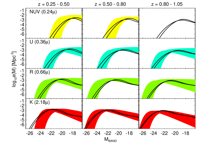
Figure 7.— Predicted luminosity function (black lines) at the minimum and maximum redshift of each redshift range shown, $z=0.25-0.5$ (left panels), $z=0.5-0.8$ (center panels), and $z=0.8-1.05$ (right panels), in the manner of Figure 4. Each is compared to observations from Cohen (2002) (except the NUV at $z=0.8-1.05$, where the observations are insufficient to determine a luminosity function), in the NUV (yellow), U (cyan), R (green), and K (red) bands.

Figure 7 extends this to higher redshift, showing the predicted luminosity function in the NUV (yellow, top panels), U-band ($0.36\,\mu$; blue, second from top), R-band (green, second from bottom), and K-band (red, bottom panels) in three redshift intervals, from Cohen (2002). Again, the shaded regions show the $1\sigma$ range in the observed luminosity function and the solid lines show our prediction at the minimum and maximum redshift of each interval. Our predictions also agree well with the VIMOS luminosity functions in U, B, V, R, and I from Zucca et al. (2005) for the redshift range $z=0.4-0.9$ (these results compare favorably with the plotted luminosity functions in the center panels).

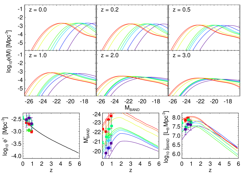
Figure 8.— Predicted luminosity function at six representative redshifts (upper left of each panel) in several bands: U (purple), B (blue), V (cyan), R (light green), I (green), J (yellow), H (orange), and K (red) (with generally decreasing characteristic magnitude). Lower panels show $\phi^{\ast}$, $M^{\ast}_{BAND}$, and $j_{\rm BAND}$ for each band, in the manner of Figure 5. Observed points for $\phi^{\ast}$, $M^{\ast}_{BAND}$, and $j_{\rm BAND}$ in U, R, and K bands are shown (filled circles of the appropriate color) from Cohen (2002), at $z=0$ from Kochanek et al. (2001) (K, red square) and Nakamura et al. (2003) (r, green triangle), and at $z=0.4-0.9$ from Zucca et al. (2005) (U, B, V, R, I, diamonds of appropriate colors).

In Figure 8, we plot the predicted luminosity function at redshifts $z=0.0,\ 0.2,\ 0.5,\ 1.0,\ 2.0,\ {\rm and}\ 3.0$, and $\phi^{\ast}$, $M^{\ast}_{BAND}$, and $j_{\rm BAND}$ (the normalization, characteristic magnitude, and total luminosity density in each band, respectively) of each luminosity function (determined as in § 4.2) for redshifts $z=0-6$. The results are shown for the bands U, B, V, R, I, J, H, and K, from purple to red, respectively. For $\phi^{\ast}$, $M^{\ast}_{BAND}$, and $j_{\rm BAND}$, the U, R, and K-band observations of Cohen (2002) (from the luminosity functions of Figure 7) are shown as filled circles (with colors matching those of the corresponding prediction for each band). The $z=0.4-0.9$ observations in U, B, V, R, I (with the corresponding colors) from Zucca et al. (2005) are shown also (diamonds), as are the $z\sim 0$ observations of Nakamura et al. (2003) (r, green triangle) and Kochanek et al. (2001) (K, red square). This provides a large set of predictions, of the shape and integrated properties ($\phi^{\ast},\ M^{\ast}_{,}j$) of the red galaxy distribution, for future comparison with red or elliptical galaxy luminosity functions.

5. The Color Distribution of Red Galaxies as a Function of Magnitude and Redshift

Figure 9 shows our predicted color-magnitude relations for several different wavebands at a series of redshifts. We plot the mean colors (lines and open diamonds) at each magnitude and redshift, with the rms dispersion in the color distribution shown as vertical error bars. We show four separate color-magnitude diagrams, for comparison with a range of observations. These are $(u-r)$ vs. $M_{r}$ (upper left), as observed in e.g., Baldry et al. (2004) and Balogh et al. (2004), $(U-V)$ vs. $M_{B}$ (upper right; Cross et al., 2004; Giallongo et al., 2005; McIntosh et al., 2005a), $(U-B)$ vs. $M_{B}$ (lower left; Willmer et al., 2005; Faber et al., 2005), and $(R-K)$ vs. $M_{K}$ (lower right; Roche et al., 2002; Pozzetti et al., 2003; Fontana et al., 2004). For $(u-r)$ vs. $M_{r}$, we show the $z=0$ color-magnitude relation determined by Balogh et al. (2004) as solid black circles, with corresponding errors. We also show the observed $(U-V)$ vs. $M_{B}$ color-magnitude relations (filled circles) at $z=0.4-1.0$ (blue) and $z=1.3-3.5$ (green) from Giallongo et al. (2005), and find reasonable agreement despite the much larger uncertainties at these larger redshifts. The $z\sim 0$ determination of $(U-V)$ vs. $M_{B}$ from McIntosh et al. (2005a) also agrees with our prediction.

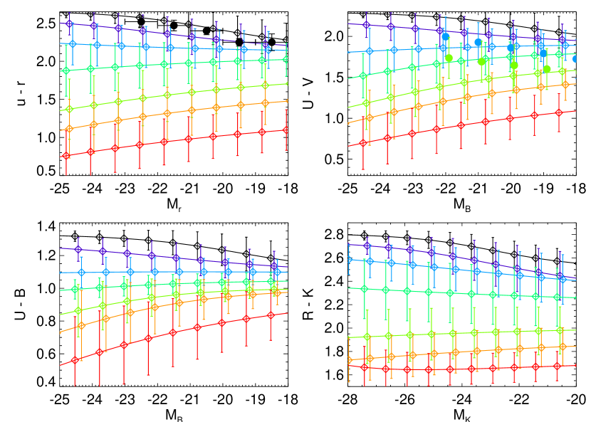
Figure 9.— Predicted mean color (diamonds and lines) as a function of magnitude for several color-magnitude pairs (as labeled), with rms deviation in the color distribution (vertical errors). Our predictions are shown for $z=0$ (black), $z=0.2$ (purple), $z=0.5$ (blue), $z=1$ (cyan), $z=2$ (green), $z=3$ (orange), $z=5$ (red), with bluer colors at higher redshift. Our results are compared to observations of $(u-r)$ vs. $M_{r}$ at $z=0$ (black circles, upper left; Balogh et al., 2004), and $(U-V)$ vs. $M_{B}$ from $z=0.4-1.0$ and $z=1.3-3.5$ (blue and green circles, respectively, upper right; Giallongo et al., 2005). Pure density evolution is assumed for the quasar luminosity function above $z\sim 2$.

We note that although our predicted $(R-K)$ colors are not as red as those of extremely red objects observed at high redshift (e.g., Roche et al., 2002; Franx et al., 2003), we are not attempting to reproduce this population, which is heavily influenced by the presence of ongoing starbursts and dust reddening, and possible AGN activity as is typical of e.g. low-redshift ultraluminous infrared galaxies (e.g., Roche et al., 2002; Miyazaki et al., 2003; Sanders & Mirabel, 1996). Our predictions are, however, consistent with the $(R-K)$ colors of ellipticals observed by, e.g., Pozzetti et al. (2003). The presence of even mild dust reddening, which we do not expect to have a large impact on most of the colors and magnitudes we show, based on the rapid falloff in column densities post-merger (Hopkins et al., 2005a), will, however, strongly redden the $(R-K)$ colors. It is therefore not surprising that our predicted, intrinsic, non-dust reddened $(R-K)$ colors are too blue, and this demonstrates that reproducing these colors will require more sophisticated models which incorporate dust reddening in the ISM and possibly the continued production of dust in stellar winds.

Our modeling reproduces the observed color-magnitude relations of red/elliptical galaxies over the range of magnitudes observed and for different observed colors. Furthermore, the typical dispersion about the mean color at low redshift, $\sim 0.2$, agrees well with that observed for this population of galaxies (Baldry et al., 2004; Balogh et al., 2004). We predict the evolution in this dispersion with redshift, in good agreement with van Dokkum et al. (2000), who find based also on the observations of Bower et al. (1992), Ellis et al. (1997), and van Dokkum et al. (1998) that the scatter in the color-magnitude [$(U-B)$ vs. $M_{B}$, specifically] relation of all progenitors of present early-type galaxies increases by a factor $\sim 2$ between $z=0$ and $z=1$. Moreover, we reproduce the observed trend of increasingly blue colors at higher redshift (e.g., Bell et al., 2004b; Cross et al., 2004; Giallongo et al., 2005) as these galaxies have formed more recently and thus not reddened as much. This is clear from the comparison with the observations of Balogh et al. (2004) and Giallongo et al. (2005) shown, but further, the observed “blueing” of the red galaxy population is observed to be $\sim 0.3$ magnitudes over the redshift range $z\sim 0-1$ (Bell et al., 2004b).

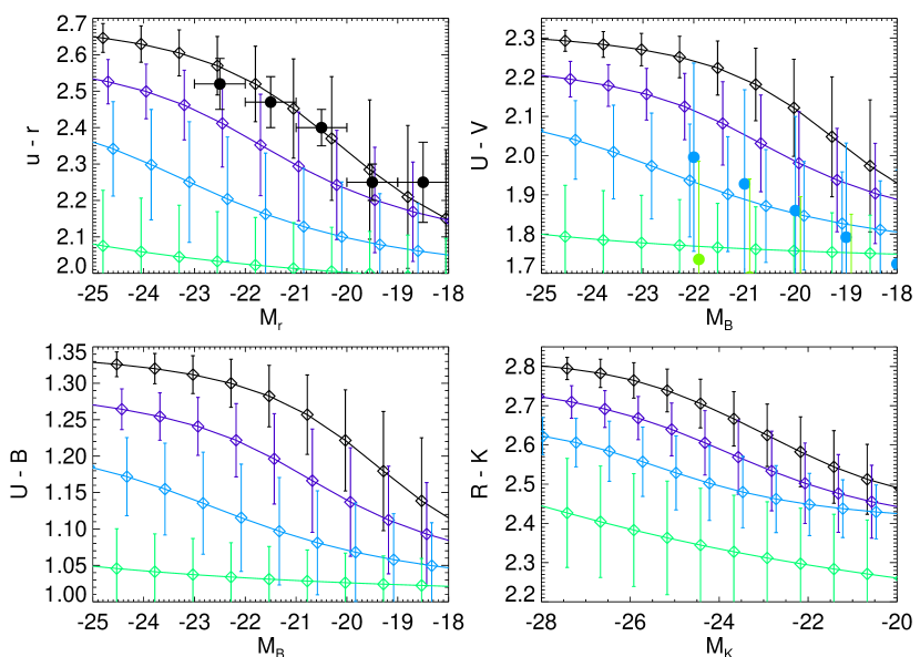
Figure 10.— Same as Figure 9, but excluding all spheroids which have formed less than 1 Gyr before the observed redshift.

At high redshifts shown in Figure 9, the slope of the color-magnitude relation changes, and brighter objects become bluer than fainter ones. The magnitude of this change in slope depends on whether we adopt a pure peak luminosity evolution (PPLE) or pure density evolution (PDE) form for the quasar evolution at high redshifts, as shown below in Figure 11. Beyond this, however, this change in slope and normalization owes to the fact that the most massive remnant galaxies form at redshifts $z\sim 2$, corresponding to the observed peak in bright quasar activity generated in mergers. Thus, at high redshift, these objects have formed more recently, and are bluer.

There is some evidence for this, as, e.g., Giallongo et al. (2005) find a $\sim 30\%$ change in the slope of the $(U-V)$ vs. $M_{B}$ relation from $z=0.4-1$ to $z=1.3-3.5$, consistent with our predictions. Still, although the observations do not strongly distinguish between the PPLE and PDE cases at this point, the weaker slope evolution seen in the PDE case is somewhat more consistent with the observations of van Dokkum et al. (2000), Bower et al. (1992), Ellis et al. (1997), and van Dokkum et al. (1998), who find results consistent with no evolution in the $(U-B)$ vs. $M_{B}$ slope at redshifts $z=0-1$, and at most a similar $\sim 30-40\%$ change over this redshift range. However, we caution that these samples are selected either by color (in which case they are obviously biased against a strong blueing of the high-mass population) or by morphology. If a considerable fraction of the most massive galaxies are still forming (i.e. have recently merged or begun merging), they will not have relaxed and will not be identified by either criterion. Therefore, we consider the color-magnitude relation derived if we ignore all objects at any redshift which have formed less than 1 Gyr in the past (about the time it takes for significant morphological and color disturbances from the merger to relax).

Figure 10 shows our predictions with this caveat (in the manner of Figure 9, also assuming pure density evolution above $z\sim 2$), for $z=0-1$, as at higher redshifts this cut excludes all but the objects formed at the highest, most uncertain redshifts. As is clear in the figure, this further reduces the evolution in the slope, with the change in slope over this redshift range in each color magnitude relation essentially consistent with zero.

We do not explicitly model populations of “old” pre-merger stars (although these are included in our simulations), which should form in the progenitor disks before the merger. Although at times long after the merger this should not be a significant contributor to the galaxy colors, as much of the stellar population is formed in a strong starburst, the effect could be significant for massive galaxies which have recently formed, reddening these objects and reducing (or even reversing) the slope evolution shown. Regardless, this slope change is difficult to observe, even in the absence of the strong limits to measured magnitudes and colors imposed from observations at higher redshift, as some of these objects become blue or morphologically disturbed enough that they will not be classified as red/elliptical galaxies. This explains our slight overprediction of the very bright end of the galaxy luminosity function at redshifts $z\gtrsim 1-2$ in § 4.1 and § 4.2, as these galaxies correspond to the rapidly blueing galaxies in these color-magnitude relations and will not appear in the observed red galaxy luminosity functions.

As noted above, we also do not include the effects of dust reddening, which can become important for recently-formed galaxies in which star formation has not yet terminated (i.e. massive galaxies at high redshift), as our modeling in Hopkins et al. (2005a) and observations of the high-redshift massive red galaxy populations (Labbé et al., 2005) indicate, and will most likely also reduce or even reverse the plotted evolution in slope. However, we do not expect this to have a strong effect on the typical mean colors at a given redshift, except perhaps for the very highest redshifts where most galaxies may still be actively merging.

Despite these caveats, we can make two further predictions from our modeling. First, the observed bimodality in the distribution of galaxy colors should break down at large redshift, especially at high luminosities, as the bright-end merger remnants become bluer. Specifically, we predict, in the absence of strong evolution in the blue color population, that the two color distributions should coalesce around $z\sim 1.5-2$, as is observed by, e.g., Willmer et al. (2005) and Giallongo et al. (2005). Second, the fraction of red galaxies (classified on the basis of the $z\sim 0$ bimodal color distribution), which dominate the bright end of the luminosity function at low redshift, should decrease at higher redshift (i.e. the bright end of the luminosity function should have an increasing contribution from “blue” galaxies, in reality the same as the red elliptical remnants observed at $z\sim 0$ but formed more recently and thus bluer), as observed by Cross et al. (2004), Daddi et al. (2004), and Somerville et al. (2004). These authors find a fraction as large as $\sim 1/3-1$ of these galaxies show irregular morphologies providing evidence for merger-driven interactions by $z\sim 1.5-2.0$, as we expect based on their formation redshifts (see also Figures 20 and 22 below). This also explains the observations of Arnouts et al. (2005) in the far UV ($1500\,$Å) from GALEX and Brinchmann et al. (1998) in HST morphological surveys, who find that the density of unobscured starburst or peculiar merging galaxies increases dramatically from $z=0$ to $z\sim 1$, where they begin to dominate the bright end of the cumulative (spiral and elliptical) luminosity function, as anticipated from the color-magnitude evolution of Figure 9 and the excess of bright blue (recently forming) galaxies beginning to appear at this redshift in Figure 4. This is also expected from our modeling of the co-production of quasars and spheroids, as numerous observations have found that the host galaxies of quasars at high redshift (which should relax to become normal present ellipticals) are excessively blue, both from AGN contributions and recent starburst activity (see, e.g. Bahcall et al., 1997; Canalizo & Stockton, 2001; Dunlop et al., 2003; Sánchez et al., 2004; Jahnke et al., 2004, and references therein). Furthermore, Labbé et al. (2005) find that dusty blue galaxies which are still forming stars constitute a large fraction ($\sim 70\%$) of the high-mass red galaxy population at $z\gtrsim 2-3$, while older “dead” red spheroids constitute a smaller fraction $\sim 30\%$, with ages implying formation redshifts $z\lesssim 5$ (accounting for a rapid quenching of star formation instead of ongoing star formation, see e.g. Förster Schreiber et al., 2004; van Dokkum et al., 2004).

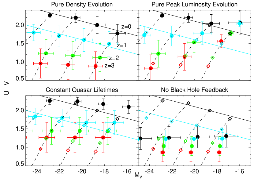
Figure 11.— Predicted mean $(U-V)$ color and $M_{V}$ magnitude (circles) with rms dispersion in color and magnitude (vertical and horizontal errorbars, respectively) as a function of redshift at $z=0$ (black), $z=1$ (blue), $z=2$ (green), and $z=0$ (red), for galaxies with total stellar mass $M_{\rm sph}=10^{9},\ 10^{10},\ 10^{11},\ {\rm and}\ 10^{12}\,M_{\sun}$, from right to left respectively. Our standard modeling, assuming pure density evolution (PDE) in the quasar population above $z\sim 2$, is shown in the upper left, with dashed lines showing the full color-magnitude tracks from $z=0$ to $z>6$. The dashed lines and PDE points from the upper left are reproduced in the other panels (diamonds), which show the mean color and magnitude with redshift assuming pure peak luminosity evolution above $z\sim 2$ (upper right), adopting a constant quasar lifetime or exponential quasar light curve (lower left), or ignoring black hole feedback in mergers (lower right). Solid line show the observed color-magnitude relations at $z=0$ (Bower et al., 1992; Schweizer & Seitzer, 1992; Terlevich et al., 2001) and $z=1$ (Bell et al., 2004b; Giallongo et al., 2005) in black and blue, respectively.

Figure 11 shows the color-magnitude [$(U-V)$ vs. $M_{V}$ shown] tracks with redshift, for the population of spheroids of fixed total stellar mass $M_{\rm sph}=10^{9},\ 10^{10},\ 10^{11},\ {\rm and}\ 10^{12}\,M_{\sun}$, from right to left, respectively (i.e. decreasing magnitude with increasing stellar mass). In the upper left, we show (dashed lines) the tracks predicted by our modeling, assuming pure density evolution for the quasar luminosity function above $z\sim 2$, from the bluest colors below the range plotted at $z\gtrsim 6$ to the reddest colors at $z=0$. The tracks show the mean color and magnitude of the population of objects at the given mass, as observed at a given redshift. For comparison, we also plot the observed $z=0$ [black; $(U-V)\approx 2.1-0.08\,(M_{V}+20)$] (Bower et al., 1992; Schweizer & Seitzer, 1992; Terlevich et al., 2001) and $z=1$ (blue; same slope but normalization lower by $\sim 0.4$ mag) (Bell et al., 2004b; Giallongo et al., 2005) color-magnitude relations as solid lines.

The agreement with the observed color-magnitude relations is good. At high redshift, galaxies of all masses are still forming, and so the mean colors are blue, and there is no significant slope in the color-magnitude diagram. However, the peak of bright quasar activity at $z\sim 2-3$ corresponds to the peak in the formation of massive spheroids via gas-rich mergers (subsequent dry merging does not affect our results). Feedback from black hole growth quenches further star formation following a merger, and the massive remnants quickly redden. However, the typical spheroids being formed shift to lower masses, as quasars evolve to smaller characteristic luminosities with decreasing redshift, keeping the population blue at lower masses, and yielding the slope of the color-magnitude diagram. This illustrates the anti-hierarchical growth of both the black hole and spheroid populations, and their self-consistency given our model of quasar lifetimes to connect the two populations.

In the upper right of Figure 11, we show the theoretical result assuming pure peak luminosity evolution (PPLE) in the quasar population above $z\sim 2$, and reproduce the pure density evolution (PDE) tracks (dashed lines) and points at redshifts $z=0,\ 1,\ 2,\ 3$ (diamonds) for comparison. At low redshifts, the agreement with observations is similar. While there is a discrepancy at the lowest masses $M_{\rm sph}=10^{9}\,M_{\sun}$, this is both where the observations are uncertain and where our prediction is sensitive to the form of the faint-end $\dot{n}(L_{\rm peak})$ [$\dot{n}(M_{\rm BH})$] distribution adopted, and, within observational uncertainty, can be slightly adjusted to yield agreement with the $z=0$ color-magnitude relation at these low masses. The evolution in the slope of the color magnitude relation is stronger in the PPLE case than the PDE case because, above $z\sim 2$, the PDE model predicts a distribution in formation rates that decreases uniformly with redshift, implying that objects of any given mass at these redshifts have the same fractional population from earlier redshifts. However, the PPLE case assumes that the distribution of formation rates shifts to lower luminosities above $z\sim 2$ rather than uniformly decreasing, implying that before $z\sim 2$, most of the lowest mass objects were formed earliest while larger objects only just formed, with this trend reversing subsequently. Because most spheroid and quasar production occurs after $z\sim 2-3$, this is sufficient to reproduce the observed $z=0$ relations, but results in the stronger slope evolution, even a reversal in sign in the color-magnitude relation slope at high redshifts. Therefore, our probes of the mean ages and in particular the age distribution of even low-redshift low-mass spheroids, as well as the color-magnitude relation at moderate and large redshifts, can constrain the evolution in the high-redshift quasar population.

In the lower left of Figure 11, we show the prediction (in the same manner as the upper right panel, again reproducing the upper left panel results of our standard modeling for comparison), assuming a constant quasar lifetime, exponential, or “on/off” model of the quasar light curve. The exact value of the quasar lifetime we chose is unimportant, as it sets only the normalization of the number of spheroids produced, not their magnitudes or color distribution. It is clear that such a model does not accurately reproduce the $z=0$ color-magnitude relation, even at moderate spheroid masses $M_{\rm sph}\sim 10^{10}-10^{11}\,M_{\sun}$. This is because such modeling does not incorporate strong enough ‘cosmic down-sizing’; i.e. a sufficiently strong age gradient with spheroid mass, even allowing for a quasar luminosity function with strong “luminosity-dependent density evolution” as e.g. the Ueda et al. (2003) luminosity function adopted here.

The lower right panel shows our predicted color-magnitude diagram neglecting black hole feedback in galaxy mergers. As demonstrated by Springel et al. (2005a), mergers without black hole feedback result in much weaker heating of the gas in the galaxy, so that star formation continues, declining in a roughly exponential manner over a Hubble time, as found in simulations without black holes by e.g. Mihos & Hernquist (1994, 1996). Therefore, we can approximate the prediction in a model neglecting black hole feedback by allowing for an exponentially declining star formation rate after a peak corresponding to the phase of quasar activity. We assume the timescale for exponential decay is $\sim 1$ Gyr, similar to that estimated in simulations neglecting black hole feedback, and demand that the stellar mass after multiple $e$-foldings is that given by e.g. our $M_{\rm BH}-M_{\rm sph}$ relation (although this choice only weakly effects our results, so long as the $M_{\rm BH}-M_{\rm sph}$ relation holds at least approximately after $\sim 1$ or more $e$-foldings in the star formation rate). The primary result of this is indicated in the lower right panel of the figure, namely that the galaxies are much too blue (by $\sim 1$ magnitude), and do not develop the characteristic slope of the color-magnitude relation. This demonstrates the dramatic importance of black hole feedback, as the rapid quenching of star formation both allows remnants to redden sufficiently and enables the gradient in formation age with mass to produce a slope in the color-magnitude relation, as opposed to its being “washed-out” by continued star formation in hosts of all masses, regardless of the peak in their star formation histories.

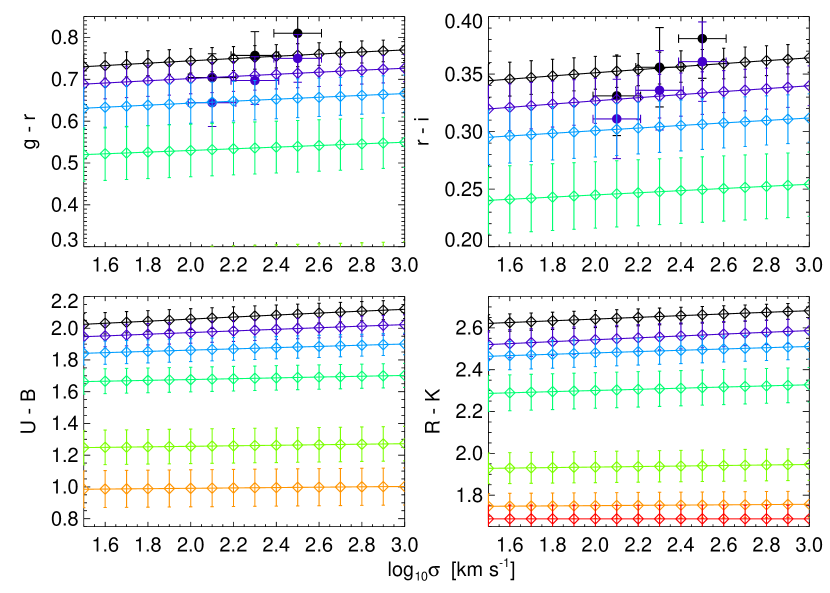
Figure 12.— Predicted mean color (diamonds and lines) as a function of spheroid stellar velocity dispersion, in the manner of Figure 9. Again, our predictions are shown for $z=0$ (black), $z=0.2$ (purple), $z=0.5$ (blue), $z=1$ (cyan), $z=2$ (green), $z=3$ (orange), $z=5$ (red), with bluer colors at higher redshift. At $z=0$ and $z=0.2$, our predicted $(g-r)$ and $(r-i)$ colors are compared to those observed as a function of velocity dispersion in Bernardi et al. (2003c, 2005).

Figure 12 shows the predicted colors of remnant spheroids as a function of spheroid stellar velocity dispersion and redshift (assuming pure density evolution above $z\sim 2$). We consider the colors SDSS $(g-r)$ (upper left) and $(r-i)$ (upper right) and the standard $(U-B)$ (lower left) and $(R-K)$ (lower right) colors. For the $(g-r)$ and $(r-i)$ colors, we compare to the color-$\sigma$ relations observed by Bernardi et al. (2003c, 2005) (filled circles) at $z=0$ (black) and $z=0.2$ (purple). Both the $z=0$ mean colors and their evolution at low redshift are reproduced by our modeling, but this is not trivial even given the $M_{\rm BH}-\sigma$ relation and fundamental plane, as for example the scatter in color is not equivalent as a function of luminosity or velocity dispersion. The dependence on velocity dispersion is also reasonably well described, with our prediction within $1\sigma$ of the observations over the range of velocity dispersion for which they exist.

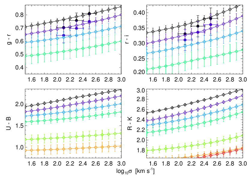
Figure 13.— Same as Figure 12, but adopting the maximal dependence of total metallicity on age and velocity dispersion from (Jørgensen et al., 1999).

The weak variation in these colors with velocity dispersion, however, means that the small effects of a systematic dependence of total metallicity on velocity dispersion or age may be important. We show the consequences of such a dependence in Figure 13, where we repeat the modeling of Figure 12, but adopt a scaling of metallicity with age (here we mean $z=0$ age, i.e. formation redshift) and velocity dispersion. To estimate the maximum effect, we consider a metallicity dependence following the strongest scaling of [Fe/H] with age and velocity dispersion found by Jørgensen et al. (1999), namely $[{\rm Fe/H}]=-0.46\,\log({\rm age/Gyr})+0.33\,\log(\sigma/{\rm km\,s^{-1}})-0.30$. We choose this scaling as opposed to others (e.g., Kuntschner, 2000) because it includes both the variation with age and velocity dispersion, but we find similar results neglecting the dependence on age. The resulting color-magnitude relations are steepened, and their slopes agree well with the observations. The colors change by a negligible amount at the approximate zero-point of the observations at $\sigma\sim 200\,{\rm km\,s^{-1}}$, because here the offset of the color-magnitude relation is determined by the ages of the spheroid populations alone, and agrees well as in Figure 12. Also, although the agreement in slope appears improved, we note that the effect is still small, generally $\lesssim 0.05$ mag in a given color even at the extreme values of $\sigma\approx 30,\ 1000\,{\rm km\,s^{-1}}$ plotted (except for the high-$\sigma$ end of the $(R-K)$ colors, which are discussed above in greater detail).

This is an approximate upper limit, for example the other determinations within Jørgensen et al. (1999) yield smaller logarithmic slopes of metallicity with $\sigma$, e.g. $\sim 0.07$ as opposed to the $0.33$ shown. That this is a still small effect and further that it serves to bring our predictions into better agreement with observations, suggests that we are safe in neglecting it in other predictions. However, with improved observations of the color-$\sigma$ variation, the distinctions between the predictions in e.g. Figure 12 and Figure 13 could be significant enough to constrain the strength of the metallicity evolution allowed or required.

We find that the scatter in colors at a given $\sigma$ is typically smaller than that at a given magnitude. In § 7 below, we demonstrate that this is a consequence of the fact that velocity dispersion is directly related to the black hole masses forming over cosmic time, whereas the $z=0$ magnitude mixes systems of different masses and ages (and thus different colors) at the same observed luminosity. Observationally, Bernardi et al. (2003c, 2005) also find that these correlations have small scatter, similar to our predictions, and argue that they are tighter and may represent a more fundamental correlation than, e.g. the color-magnitude relations. We also note that the qualitative behavior of colors as a function of velocity dispersion and redshift is similar for each of the colors considered, although different colors are rescaled about different values, and the evolution in the slope of the color-$\sigma$ relation is much weaker than that of the color-magnitude relation. These properties make the color-velocity dispersion relation a valuable probe not just as a check on the color-magnitude relation but potentially as a measurement independent of some systematics (for example, the common observational assumption of constant slope with redshift in this case appears quite reliable).

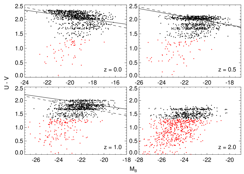
Figure 14.— Predicted $(U-V)$ vs. $M_{B}$ color-magnitude relation at redshifts $z=0,\ 0.5,\ 1,\ {\rm and}\ 2$, as labeled. In each panel, 1000 galaxies are generated according to the predicted joint color-magnitude distributions at the given redshift. Black points show galaxies older than 0.5 Gyr, red points younger. In the upper left, the solid line shows the best-fit color-magnitude to our predictions, the dashed line the best-fit to the observed galaxies from Bell et al. (2004b); Giallongo et al. (2005). In the upper right and lower left, the solid line shows the observed color-magnitude relation of Giallongo et al. (2005), dashed line the observed relation of Bell et al. (2004b).

Finally, we use our modeling to generate an observed color-magnitude relation in Figure 14. At each redshift considered, we calculate the joint probability distribution in both color and magnitude based on our predicted history of spheroid formation prior to that redshift (i.e. the color distribution at a given magnitude in Figure 9, and distribution in magnitudes from our predicted luminosity functions in e.g. Figure 4), and generate 1000 points (mock galaxies) according to that probability distribution. These are not full simulated galaxies, but random points drawn from our calculated joint PDF in color and magnitude at each redshift. At $z=0$, we directly fit the generated points to a color-magnitude relation, and show the result, $(U-V)=1.9-0.04\,(M_{B}+20)$ as a solid black line. Our result is similar to the observed relation, $(U-V)=2.1-0.08\,(M_{B}+20)$ from Bell et al. (2004b) and Giallongo et al. (2005), as is the absolute distribution in magnitude and color. We show galaxies older than 0.5 Gyr as black points, and galaxies younger than this as red points. This demonstrates that very young galaxies are not a significant contributor to the observed red galaxy population at low redshift, and thus the fact that they lie in a more blue, brighter region of color-magnitude space than the “normal” relaxed elliptical population, as well as most likely being disturbed systems which would not be morphologically recognized as ellipticals, is not important in our calculations at low redshift. The removal of these points at $z=0$ does not change our results significantly, except to slightly steepen the fitted color-magnitude slope to $-0.06$, in better agreement with that observed.

At $z=0.5$ and $z=1$, the fractional “young” population is still relatively small, although it does increase, and the observed color-magnitude relations still agree well with our predicted distribution of “old” elliptical colors and magnitudes. We show the observed color-magnitude relations of Bell et al. (2004b), who assume a constant slope at all redshifts, at these redshifts as dashed lines, and the observed relation of Giallongo et al. (2005), who allow the slope to vary, as solid lines. As shown in Figure 10, we reproduce the observed evolution in the red/elliptical color-magnitude relations if we restrict ourselves to the older spheroids which have had sufficient time after their progenitor gas-rich mergers to relax and be recognized as ellipticals by either color or morphological selection criteria. By $z=2$ (lower right), however, the fraction of young objects becomes quite large ($\approx 0.5$), as observed and discussed further above and in § 7.

6. Spheroid Mass to Light Ratios and Luminosity-Size Relations as a Function of Mass and Redshift

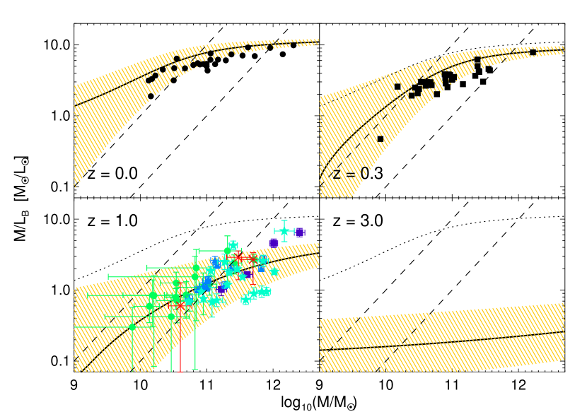
Figure 15.— Predicted mean mass to B-band light ratio $M/L_{B}$ (solid lines) as a function of spheroid mass $M$, with $1\sigma$ dispersion at each $M$ (yellow shaded region). Results are shown for $z=0$ (upper left), $z=0.3$ (upper right), $z=1$ (lower left), and $z=3$ (lower right), as labeled. Observations at $z\approx 0$ (black circles) are from Jørgensen et al. (1995a, b, 1996), at $z\approx 0.3$ (black squares) from Kelson et al. (2000), and at $z\approx 1$ from van der Wel et al. (2005) (cyan stars), Holden et al. (2005) (purple squares), van Dokkum & Stanford (2003) (red $\times$’s), Wuyts et al. (2004) (blue triangles), and di Serego Alighieri et al. (2005) (green circles). Luminosity limits of $10^{10}\,L_{\sun}$ and $10^{11}\,L_{\sun}$ are shown in each panel (dashed lines), as is the $z=0$ mean $M/L_{B}$ (dotted lines).

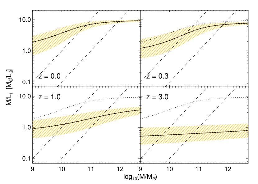
Figure 16.— As Figure 15, but our predictions are shown for the mass to I-band mass to light ratio $M/L_{I}$.

Figure 15 shows our predicted $M/L$ ratio in the B-band ($M/L_{B}$) as a function of spheroid mass. For each redshift, we use our modeling of $\dot{n}(M_{\rm BH})$, $\dot{n}(M_{\rm sph})$ from the quasar luminosity function to determine the distribution of ages for spheroids of a given mass at that redshift, and from that determine the distribution of $M/L$ ratios in a given band. The masses shown are $M_{\rm vir}$, the virial mass within the effective radius ($\equiv 5\sigma^{2}R_{e}/G$, as defined in § 2.3), in order to ease comparison with observations (which generally adopt this choice; those that do not have been rescaled accordingly).

Our $z=0$ prediction is compared to observations of spheroids in the Coma cluster (at $z=0.023$) from Jørgensen et al. (1995a, b, 1996) (black circles), which are similar to recent determinations from the SDSS and other studies (e.g. van der Wel et al., 2005; Cappellari et al., 2005). The $z=0.3$ result is compared to observations of the cluster Cl 1358+62 at $z=0.33$ from Kelson et al. (2000) (black squares). Our $z=1$ prediction is compared to several different observations, including those from $0.6<z<1.15$ in the Chandra Deep Field-South sample of van der Wel et al. (2005) (cyan stars), the $z=1.237$ cluster RDCS 1252.9-2927 sample of Holden et al. (2005) (purple squares), the $z=1.27$ cluster RDCS J0848+4453 galaxies from van Dokkum & Stanford (2003) (red $\times$’s), the $z=0.83$ cluster MS 1054-03 sample of Wuyts et al. (2004) (blue triangles), and the $0.88<z<1.3$ K20 sample of di Serego Alighieri et al. (2005) (green circles). In each panel at $z>0$, we show the $z=0$ mean $M/L_{B}$ prediction for comparison (dotted lines). We also show our predicted mass to I-band light ratios $M/L_{I}$ as a function of mass in Figure 16, in the same manner as Figure 15, demonstrating the relative importance of different age distributions in different observed wavebands.

Our modeling reproduces the typical $M/L_{B}$ ratios and their dependence on mass, and the scatter about the mean $M/L_{B}$, which increases significantly with increasing redshift and decreasing mass. Although for clarity we have not shown other redshifts, we have compared e.g. the $z=0.58$ MS 2053-04 sample of Wuyts et al. (2004) to our predictions and find similar agreement. Our modeling further predicts the observed differential evolution in $M/L_{B}$, where the mass to light ratio declines more rapidly with redshift above $z=0$ in smaller-mass systems, implying that these formed more recently (see, e.g. Treu et al., 2001; van Dokkum et al., 2001; Treu et al., 2002; van Dokkum & Stanford, 2003; Gebhardt et al., 2003; Rusin et al., 2003; van de Ven et al., 2003; Wuyts et al., 2004; Treu et al., 2005; Holden et al., 2005; van der Wel et al., 2005; di Serego Alighieri et al., 2005). At $z\gtrsim 2$, our model agrees well with the observations, for example the mass-to-light ratio as a function of mass in the K-band of distant red galaxies found by Labbé et al. (2005), which may even observe the flattening in the $M/L$ relation we predict for $z\gtrsim 2-3$, although it is difficult to determine this given luminosity limits at these high redshifts. These observations suggest that many of the most massive galaxies are forming at this redshift, with $\sim 70\%$ of the population being blue, dusty galaxies still forming stars at a high rate (Labbé et al., 2005), as we expect (see § 7 for a more detailed discussion) and a fraction of the most massive galaxies formed as early as $z\sim 5$, although this age is lower than estimated in e.g. Labbé et al. (2005) if we account for the rapid quenching of star formation seen in our simulations in modeling the stellar populations (e.g. Förster Schreiber et al., 2004; van Dokkum et al., 2004).

Our modeling suggests that the $M/L_{B}$ relation should steepen below $M\sim{\rm a\ few}\ \times 10^{10}\,M_{\sun}$, where at low redshift, samples are severely limited by luminosity/magnitude limits, making the differential evolution slightly less dramatic. However, we caution against interpreting this curvature too strictly, as it depends on both the functional form and quantitative dependence of the quasar luminosity function break luminosity on redshift. In our adopted form for the quasar luminosity function, the break luminosity evolves exponentially with lookback time, in which case the degree of curvature is quite sensitive to the coefficient of this exponential growth, whereas if e.g. we considered exponential evolution in redshift (instead of lookback time), we obtain similar values of $M/L_{B}$ at small and large $M$, but with a less curved power-law interpolation between them.

To illustrate the impact of selection effects, we plot (dashed lines) the lower observable mass limit for a limiting luminosity of $10^{10}\,L_{\sun}$ (left) and $10^{11}\,L_{\sun}$ (right) in each panel. The scaling we describe in § 2.3 between virial and stellar mass within the effective radius (or stellar mass and effective radius) is a non-negligible component of the $z=0$ slope of the $M/L$ ratio – ignoring this scaling does not change our predictions at the high-mass end, but results in an overprediction of the $M/L$ ratio at the low-mass end by a factor $\sim 2$. However, the redshift evolution is almost entirely a consequence of the different ages of spheroids of different mass; our predictions for the differential $M/L$ evolution with redshift are essentially identical if we neglect the weak evolution in the $M_{\rm sph}-R_{e}$ relation with redshift described in Robertson et al. (2005c, in preparation).

Differential evolution in the $M/L_{B}$ ratio is expected in our model because the break in the quasar luminosity function shifts to lower luminosities below $z\sim 2-3$, implying that spheroids with smaller black hole mass (smaller peak luminosity) are dominating the distribution of objects being formed at these later times. Therefore, at $z\sim 1$, the lower mass objects have formed more recently. However, above $z\sim 2-3$, this differential evolution should either flatten or reverse, if a pure density or pure peak luminosity evolution model of the quasar luminosity function is an accurate description of quasar activity. The results in Figure 15 assume pure density evolution in the quasar luminosity function above $z\sim 2$. In this case, above $z\sim 2$, the shape of the luminosity function (and therefore, the distribution of peak luminosities and corresponding spheroid masses being formed) remains constant, and the normalization decreases with higher redshift. Thus, all objects have the same distribution of formation ages above this redshift (with only second-order effects from the finite quasar lifetime and merger time, at least until high redshifts where these times become comparable to the Hubble time). Therefore, the slope of $M/L_{B}$ vs. $M$ should become flat (except for the small effects of the $M_{\rm sph}-R_{e}$ relation), as seen in the figure for $z=3$.

In a pure peak luminosity evolution scenario, the shape of the quasar luminosity function above $z\sim 2$ again remains roughly constant, but instead of decreasing in normalization, the break luminosity shifts to smaller luminosities at higher redshifts, with constant normalization. This implies that, above $z\sim 2-3$, the more massive objects have actually formed more recently, and so the slope of the $M/L_{B}$ vs. $M$ relation should be inverted, i.e. that $M/L_{B}$ should decrease with mass. However, if metallicity evolves with either mass or redshift, this will affect the mean mass to light ratio and slope as well, although we discuss this effect above and show in Figure 13 that it is small.

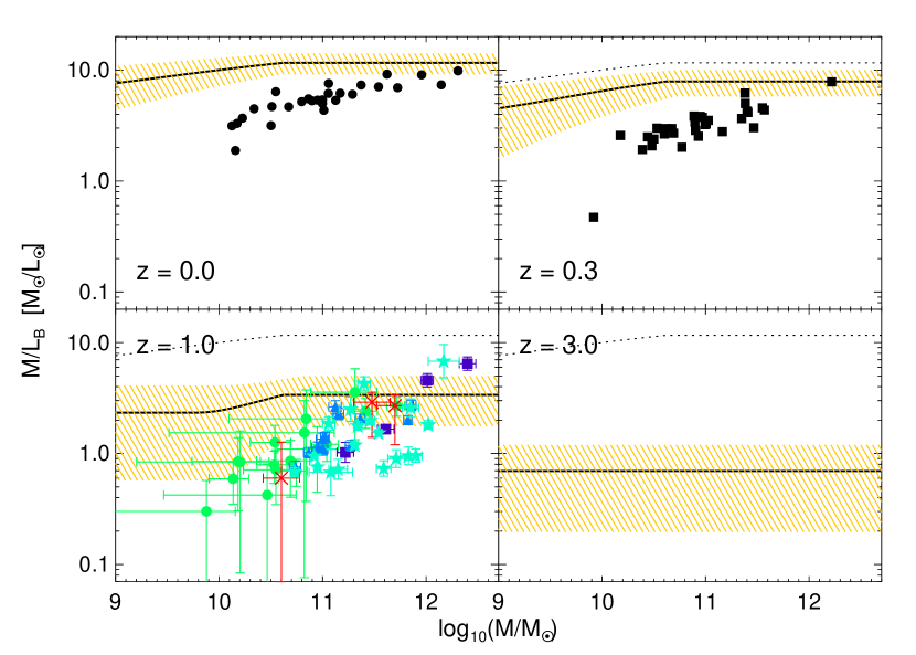
Figure 17.— As Figure 15, but assuming a “light-bulb” (“on/off”) or pure exponential model of the quasar light curve and lifetime.

We also test whether the distributions of spheroid mass to light ratios inferred from idealized models of the quasar lifetime are consistent with observations. We consider a case in which quasars have a fixed, constant lifetime and radiate at a fixed luminosity $L=L_{\rm peak}$. Here, the value of the quasar lifetime is unimportant, as it controls only the normalization of the resulting rates of spheroid formation. We adopt the luminosity function of Ueda et al. (2003), from the hard X-ray, modified for pure density evolution above $z=2$ following Fan et al. (2001), although our results are qualitatively insensitive to these specific choices (Hopkins et al., 2005c). We have already demonstrated in Figure 4 and Figure 11 that such modeling predicts a spheroid luminosity function and color-magnitude relation in stark disagreement with observations.

Figure 17 shows the predicted B-band mass to light ratios $M/L_{B}$ as a function of mass at redshifts $z=0,\ 0.3,\ 1,\ 3$, in the same manner as Figure 15 and with the same observations shown, but adopting this idealized model for the quasar light curve. The predicted mass-to-light ratio is too high by a factor $\sim 2-5$ at all but the largest masses, and shows almost no dependence on mass at any redshift, and no differential evolution from $z=0$ to $z=1$. Although both the color-magnitude relation and mass to light ratios derive from the same underlying age distribution, the distinction between the predictions of our full model of quasar activity and idealized models is significantly stronger in the predicted mass to light ratios than color magnitude relations (Figure 11). We note that the Ueda et al. (2003) luminosity function does include “luminosity-dependent density evolution,” in which the slope of the faint-end quasar luminosity function evolves with redshift, implying that the density of lower-luminosities quasars peaks at lower redshift. This is the only reason, in fact, that there is any dependence of $M/L_{B}$ on $M$ at all in Figure 17. Although this is qualitatively consistent with the anti-hierarchical, downsizing picture implied by the observations described above, the figure demonstrates that it is quantitatively insufficient to account for the downsizing observed in the spheroid population.

At high redshifts $z\sim 2$, traditional models of the quasar luminosity function associate an observed luminosity with a quasar’s peak luminosity, implying that many low-peak luminosity (i.e. low final black hole mass and, correspondingly, small spheroid mass) systems are forming at these redshifts. Even if the inferred formation of these objects reaches a maximum at somewhat lower redshift, they are still formed over a wide range of redshifts with a large number of the smallest-mass systems formed at $z\sim 1-3$. However, in our model these observed faint-end objects are really brighter peak luminosity sources, in a dimmer stage of their evolution; the distribution of peak luminosities being formed at a given redshift is actually peaked, at a luminosity corresponding the break in the observed luminosity function. Thus, low peak luminosity systems (small spheroid masses) are not formed until much later times, when the break luminosity has evolved to small luminosities. In fact, in our modeling, the observed change in quasar luminosity function slope is actually a consequence of the quasar lifetime as a function of luminosity, while the break luminosity evolution reflects “cosmic downsizing” (Hopkins et al., 2005f).

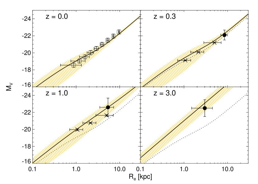
Figure 18.— Predicted luminosity-size relation (in V-band) at several redshifts, as labeled. The mean luminosity-size relation (black lines) and $1\sigma$ range (yellow shaded area) are shown. Dotted lines in each panel show the mean $z=0$ relation. Observations at $z=0$ (squares) are from Shen et al. (2003), with horizontal error bars showing the dispersion in $R_{e}$ at each constant $M_{V}$. Observations at $z>0$ are from Trujillo et al. (2005, circles) and McIntosh et al. (2005b, $\times$’s).

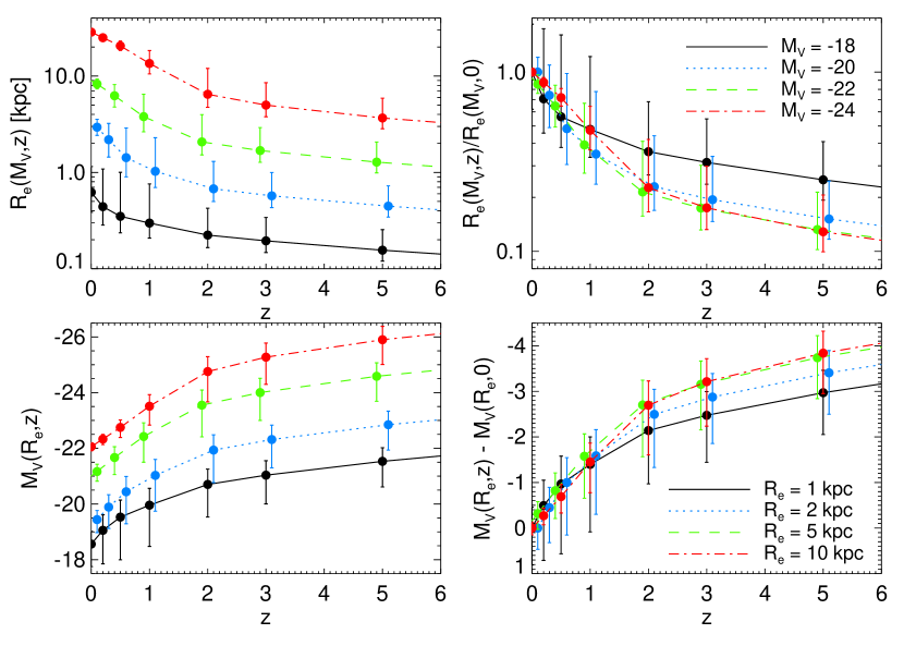
Figure 19.— Predicted luminosity-size relation (in V-band) as a function of redshift. Upper panels show the absolute (left) and relative (normalized to the $z=0$ value, right) effective radii $R_{e}$ (and $1\sigma$ range of radii, vertical error bars) as a function of redshift, at fixed luminosity ($M_{V}=-18,\ -20,\ -22,\ -24$, as labeled). Lower panels show the absolute (left) and relative (right) V-band magnitude (and $1\sigma$ range of magnitudes, vertical error bars) as a function of redshift, at fixed effective radius ($R_{e}=1,\ 2,\ 5,\ 10$ kpc, as labeled).

As discussed in § 2.3 above, Robertson et al. (2005c, in preparation) analyze scaling relations for merger remnants and their implications for the fundamental plane. However, that work considers only the structural properties of individual objects and does not predict the age distribution of any population. Here, we determine the distribution of spheroid ages as a function of e.g. stellar mass, and combine this with knowledge of the detailed structure of the remnants to predict the observed luminosity-size relations as a function of redshift in bands where mass to light evolution is important. For present purposes, we emphasize that our simulations reproduce well the observed $z=0$ effective radius-stellar mass relation of remnant red/elliptical galaxies (e.g. Bernardi et al. 2003a, Shen et al. 2003; Padmanabhan et al. 2004; Cappellari et al. 2005), as well as predicting that this relation should evolve at most weakly with redshift, in agreement with observations (Trujillo & Aguerri, 2004; Trujillo et al., 2004, 2005; McIntosh et al., 2005b) (see also e.g. Ferguson et al., 2004; Bouwens et al., 2004; Papovich et al., 2005, although these authors do not separate the relation by morphological type). Given a nearly redshift-independent $R_{e}-M_{\rm sph}$ relation, it is then straightforward to convert our predicted mass-to-light ratios as a function of mass to a luminosity-size relation (luminosity as a function of effective radius). This then enables a secondary means of measuring the relative ages and differential evolution of the remnant spheroid population, which in many cases probes different regimes in size and redshift.

Figure 18 shows the resulting predicted luminosity-size relation (in V-band) at several redshifts. We compare to observations at $z=0$ (squares) from Shen et al. (2003), with horizontal error bars showing the dispersion in $R_{e}$ at each constant $M_{V}$. These observations are converted from the r-band using our predicted color-magnitude relations (§ 5), which further implicitly guarantee that we reproduce the observed luminosity-size relation in all other wavebands. Further observations at each $z>0$ are shown from Trujillo et al. (2005, circles) and McIntosh et al. (2005b, $\times$’s).

Our modeling reproduces both the mean luminosity-size relation at each redshift, as well as the range of $R_{e}$ at fixed luminosity as a function of luminosity (compare the $z=0$ dispersions from Shen et al. (2003) and our modeling). For the observed redshift ranges, the effect of the change in the $M_{\rm sph}-R_{e}$ relation with redshift in our simulations is small, for example at fixed $M_{\rm sph}=10^{10}\,M_{\sun}$ the effective radius decreases by just $25\%$ from $z=0$ to $z=2$, and the evolution in the luminosity-size relation is driven primarily by evolution in mass-to-light ratios owing to different spheroid ages as a function of mass or size.

We show the evolution with redshift of both effective radius at fixed luminosity and luminosity at fixed effective radius in greater detail in Figure 19. The points at each magnitude are offset by a negligible amount for clarity. Although the interpretation is not as straightforward as that of our mass-to-light ratio predictions, the more rapid and pronounced relative magnitude evolution of systems with larger effective radii is a reflection of the same anti-hierarchical growth discussed above (and below in § 7), with larger (higher-mass) systems forming at higher redshift.

7. Galaxy Ages as a Function of Mass and Luminosity

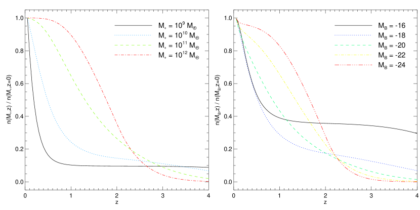
Figure 20.— Predicted fraction of $z=0$ spheroids with stellar mass $M_{\ast}$ formed by a given redshift as a function of redshift, for $M_{\ast}=10^{9},\ 10^{10},\ 10^{11},\ {\rm and}\ 10^{12}\,M_{\sun}$, as labeled (left). Right panel shows the same, but for spheroids observed at $z=0$ with a given B-band magnitude $M_{B}=-16,\ -18,\ -20,\ -22,\ -24$, as labeled.

Figure 20 shows the fraction of all $z=0$ spheroids of a given stellar mass formed by a given redshift, as a function of redshift for spheroid stellar masses $M_{\ast}=M_{\rm sph}=10^{9},\ 10^{10},\ 10^{11},\ {\rm and}\ 10^{12}\,M_{\sun}$. Given the anti-hierarchical nature of black hole growth described in Hopkins et al. (2005e), where the highest-mass black holes are formed at high redshifts, associated with the peak in bright quasar activity, and lower mass black holes are formed at lower redshift as the break in the observed quasar luminosity function (corresponding to the peak in the formation rate of final black hole masses $\dot{n}(M_{\rm BH})$) moves to lower luminosities, we expect the trend indicated, where higher-mass spheroids are formed at higher redshifts and over a wider range in redshift, as these correspond to higher-mass black holes.

This evolution in black hole mass explains the observations of Bernardi et al. (2003c, 2005), who find that color is primarily correlated with velocity dispersion (see Figure 12), with the color-magnitude relations discussed above being a consequence of the fact that magnitudes are also correlated with velocity dispersion. Based on the quasar luminosity function, the dispersion in ages for a given $\sigma$ is small, as black holes of a given mass form over a well-defined range of redshifts. Since feedback from black hole growth results in passive evolution of the remnant after quasar activity, the age (and therefore reddening) of the remnant is correlated more tightly with the velocity dispersion (i.e. black hole mass) of the remnant than its luminosity (magnitude), which mixes galaxies of different black hole masses and ages.

Figure 20 also shows the fraction of all $z=0$ spheroids of a given B-band magnitude formed by a given redshift. Unlike the fractional population vs. redshift as a function of mass, this includes the effects of stellar evolution, effectively mixing e.g. older, more massive galaxies with younger, less massive ones that have the same $z=0$ B-band luminosity. Despite this, the trend of higher luminosity objects forming at characteristically larger redshifts and over a wider range of redshifts is clear. The flattening of the lowest-luminosity population growth at $z\sim 1$ is a consequence of the pure peak luminosity evolution model for the quasar luminosity function evolution at $z\gtrsim 2$. With pure density evolution above $z\sim 2$, the lowest luminosity curve will continue to fall rapidly, without a significant number of very low peak luminosity (low spheroid mass) systems forming at high redshift.

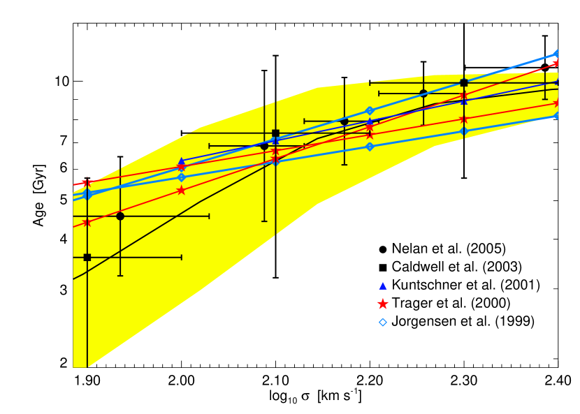
Figure 21.— Predicted $z=0$ ages of spheroids as a function of velocity dispersion. Black solid line shows our predicted median age, yellow range shows the interquartile range of ages at each $\sigma$. Observations of mean age (and dispersion about the mean, vertical error bars) in bins of $\log\sigma$ are shown from Nelan et al. (2005) (circles) and Caldwell et al. (2003) (squares), and the $\sim 1\sigma$ range of fitted age-$\sigma$ relations from Kuntschner et al. (2001) (dark blue line with triangles), Trager et al. (2000) (red line with stars), and Jørgensen (1999) (light blue line with diamonds) are shown as solid lines.

In Figure 21, we plot the predicted $z=0$ ages of spheroids as a function of velocity dispersion from our modeling (assuming pure peak luminosity evolution at $z\gtrsim 2$, although this only becomes important here at very low $\sigma$ where the range of ages is relatively large in either case). Observations of the mean age in bins of $\log\sigma$ are shown from Nelan et al. (2005) (circles) and Caldwell et al. (2003) (squares), with horizontal errors showing the range of $\log\sigma$ of each bin and vertical error bars showing the rms dispersion in ages at the given velocity dispersion (which can be compared to the yellow range plotted). The $\sim 1\sigma$ range of fitted age-$\sigma$ relations (i.e. adopting the minimal and maximal fitted age-$\sigma$ slopes) from Kuntschner et al. (2001) (dark blue line with triangles), Trager et al. (2000) (red line with stars), and Jørgensen (1999) (light blue line with diamonds) are shown as solid lines. The slopes from the observations of Kuntschner et al. (2001) and Trager et al. (2000) are determined by fitting in Nelan et al. (2005).

The agreement at all values of $\sigma$ is good, again implying that the downsizing of both galaxy and quasar populations is self-consistent when our model of the quasar lifetime is adopted, and emphasizing that age evolution as a function of velocity dispersion or stellar mass is important along the red sequence (i.e. that the red sequence is not merely a metallicity sequence). There is a slight systematic offset in the mean age, with several of the observations estimating ages $\sim 1\,$Gyr larger than those we predict, but this is well within the uncertainties of both our theoretical modeling and observational estimates of absolute ages.

Our prediction of the age-velocity dispersion relation includes the observed steepening of the relation at low velocity dispersions (e.g., Caldwell et al., 2003; Nelan et al., 2005), an effect not accounted for in fitting a single power law, which is why the power law fits extrapolated to low $\sigma$ tend to predict larger ages than given by either our prediction or the binned observations. There is also a suggestion that the dispersion in age becomes larger at low velocity dispersion, an effect discussed in detail in § 5, and potentially seen in some observations (e.g. Nelan et al., 2005), but the observations are still uncertain on this point and as shown in regard to the color-magnitude relation, this effect can be quite sensitive to whether pure peak luminosity or pure density evolution is assumed for the quasar population at high redshift.

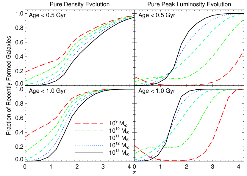
Figure 22.— Predicted fraction of spheroids of a given total stellar mass (as labeled) with ages less then either 0.5 Gyr (upper panels) or 1.0 Gyr (lower panels), as a function of redshift. Left panels assume pure density evolution in the quasar population above $z\sim 2$, right panels assume pure peak luminosity evolution.

Figure 22 considers the population of very recently formed spheroids, which will not yet be relaxed or reddened and may be identified as either peculiar or interacting galaxies. We determine the fraction of spheroids with ages less than 0.5 Gyr (upper panels) or 1.0 Gyr (lower panels), as a function of redshift. In the left and right panels, we show this prediction assuming either pure density or pure peak luminosity evolution of the quasar population above $z\sim 2$, respectively. The predictions are similar for a limiting age of both 0.5 and 1.0 Gyr; that our predictions are not strongly sensitive to the spheroid age in this regime suggests that this can be observationally measured via relatively simple diagnostics. Clearly, direct measures of the population of merging and interacting galaxies probe the fraction of galaxies with very recent formation times, but by $\sim 1$ Gyr, many of these objects may be identified not through more difficult morphological analysis but e.g. through spectral classification as K+A galaxies.

Moreover, the fraction of young objects at e.g. $z=3$ is sensitive to the strength of the density evolution modeled, which allows observations of the distribution of spectral types as a function of redshift to not only test our modeling but also to constrain the form of high-redshift quasar evolution. While at very low redshift the results are similar, the prediction that the fraction of young objects should be higher in low-mass spheroids reverses rapidly at $z\sim 1$ in the pure peak luminosity evolution case. This distinction should allow even rough observations of the fraction of K+A vs. A galaxies at $z\gtrsim 1-2$ to break the observational degeneracy between pure density and pure peak luminosity evolution.

Bernardi et al. (2003c) find from the color and chemical evolution of SDSS elliptical galaxies that these galaxies are passively evolving at redshifts $z\lesssim 0.5$, and that they (on average) formed $\sim 9$ Gyr in the past. Bernardi et al. (2003a, b) determine the same characteristic age independently based on analyses of the fundamental plane and $z=0$ galaxy scaling relations. This corresponds to a redshift of formation $z\sim 1.5$, consistent with our predictions for the formation redshifts of massive red galaxies. This age also makes it clear that the peak elliptical galaxy formation occurs contemporaneously with peak quasar activity at $z\sim 2$, which is explained if spheroids and quasars form together.

This is also consistent with direct observations of the morphologies of galaxies, which show that by $z\sim 0.7$ red galaxies are almost all relaxing ellipticals, with little contribution to observed luminosity from e.g. dusty spirals (Bell et al., 2004a). Fontana et al. (2004) also find similar results from studying ellipticals in the K20 survey; namely, that massive ellipticals evolve passively for $z\lesssim 0.7$, with little growth in the total mass density in spheroids. However, at $z\gtrsim 1$, the mass growth in ellipticals rises steeply, with most mass assembly at $z\sim 1-2$. Specifically, they estimate $\sim 1/3$ of the present mass of massive ellipticals has been assembled recently by $z\sim 2$, in agreement with our predictions for the evolution of the stellar mass function and ages (Figures 3, 20, and 22). They further find that for $z\gtrsim 1$, the $z=0$ population of massive ellipticals becomes increasingly dominated by star-forming galaxies, as expected in a merger-driven scenario for contemporaneous spheroid and quasar formation. Likewise, Somerville et al. (2004) and Daddi et al. (2004) observe that at $z\sim 1.5-2$, the massive elliptical population includes large numbers of highly disturbed morphologies indicative of merger-induced starbursts. Cross et al. (2004) find from fundamental plane analyses that the production of massive red ellipticals should increase with cosmic time to a peak at $z\sim 2$ and then fall, suggesting that this is the epoch of peak massive spheroid formation. This is also supported by direct observations of quasar host galaxies, which find strong evidence for simultaneous and strongly associated black hole growth and star formation at redshifts corresponding to peak quasar activity ($z\gtrsim 1$) (e.g., Alexander et al., 2005).

Many observations indicate that galaxy age increases with velocity dispersion or spheroid mass (e.g., Jørgensen, 1999; Trager et al., 2000; Kuntschner et al., 2001; Caldwell et al., 2003; Fontana et al., 2004; Bernardi et al., 2005; Faber et al., 2005; Howell, 2005; Tanaka et al., 2005; Gallazzi et al., 2005; Nelan et al., 2005), as we have considered in Figure 21. Gallazzi et al. (2005) also quantify this trend in terms of stellar mass, finding that galaxies with mass $\sim 10^{9}-10^{12}\,M_{\sun}$ form at redshifts $z\sim 1.5-2$, with median age increasing systematically with mass; they estimate e.g. $\sim 16\%$ of $10^{12}\,M_{\sun}$ galaxies (at which point their sample is spheroid-dominated) are in place by $z\sim 2$, rising to $\sim 50\%$ at $z=1.8$, similar to our predictions in Figure 20. This is a consequence of the strong anti-hierarchical black hole growth implied by our interpretation of the quasar luminosity function, where higher-mass black holes (thus higher-$\sigma$ spheroids) form at higher redshift $z\sim 2$, and thus we reproduce both the mean age of $z=0$ spheroids and its evolution with velocity dispersion and mass. These authors also find that higher velocity dispersion does not imply strongly decreasing metallicity, which is consistent with our picture of rapid metal enrichment (even at high redshift) in the starburst phase of the merger.

Our results are consistent with ages inferred from fundamental plane analyses (e.g., van Dokkum & Franx, 1996; Jørgensen et al., 1996, 1999; van Dokkum et al., 1998, 1999, 2000, 2001; Treu et al., 2001, 2002; Gebhardt et al., 2003; Cross et al., 2004; Wuyts et al., 2004; van de Ven et al., 2003), color and spectral analyses (e.g., Bower et al., 1992; Ellis et al., 1997; Bernardi et al., 1998; Stanford et al., 1998; Ferreras et al., 1999; Schade et al., 1999; Menanteau et al., 2001; Kuntschner et al., 2002; Treu et al., 2002; Pozzetti et al., 2003; van de Ven et al., 2003; Bell et al., 2004b; Förster Schreiber et al., 2004; Labbé et al., 2005), and gravitationally lensed objects (e.g., Rusin et al., 2003; Rusin & Kochanek, 2005). These all indicate typical formation redshifts $z\sim 1.5-2.5$, with a large range of formation redshifts $\Delta z\sim 1.5-2.0$ (Treu et al., 2001, 2002; van de Ven et al., 2003; Cross et al., 2004; Rusin & Kochanek, 2005), and subsequent passive evolution of reddening remnant ellipticals. Although semi-analytical models of hierarchical galaxy formation reproduce this as a general trend in the star formation history of the Universe, recent results by Menci et al. (2005), which attempt to reproduce the observed bimodal color distribution of galaxies, predict that red galaxies formed only in dense environments, underpredicting the relative red field galaxy population and the number of faint red galaxies. Furthermore this semi-analytical modeling predicts that red galaxies form at much too high a redshift, $z\sim 4-5$. Explicitly, Daddi et al. (2004) find that the number density of massive spheroids which are forming and should appear as highly disturbed starbursting galaxies at $z\sim 2$ is underpredicted by a factor of at least $\sim 30$ by current semi-analytical models.

A key ingredient in resolving this discrepancy is clear from the results of Springel et al. (2005a), who show that feedback from black hole growth and quasar activity is critical in rapidly terminating star formation, allowing the production of quiescent red ellipticals even from mergers of relatively low-mass (faint) objects at much lower redshifts and explaining the observations of more recent formation redshifts $z\sim 2$. Furthermore, the presence of a massive black hole is also important in maintaining continued reddening of the elliptical, as feedback from residual accretion can re-heat the gas, suppressing further star formation after the merger. This is also suggested directly by the comparison between luminosity functions and the modeling of Nagamine et al. (2001), Menci et al. (2004), and Granato et al. (2004) in Fontana et al. (2004), who show that these models under or over-predict the bright luminosity function at high redshift, but that AGN feedback can regulate the slope of the galaxy stellar mass function at low masses. It is also important to note that even those models which incorporate black hole growth and feedback (e.g. Granato et al., 2004) must properly model the quasar lifetime and its dependence on luminosity (Hopkins et al., 2005c, e) in order to simultaneously reproduce the quasar and red galaxy luminosity functions and other properties in any picture of merger-driven AGN activity, as we demonstrate in Figures 4, 11, and 17.

8. Conclusions

Here, we have considered the consequences of a merger-driven scenario for the joint formation of spheroids, quasars, and relic supermassive black holes for the population of red galaxies. As we demonstrate elsewhere, the remnant spheroid hot X-ray emitting gas properties (Cox et al., 2005a), morphologies (Cox et al. 2005b, in preparation), metallicities (Cox et al. 2005c, in preparation), $M_{\rm BH}-\sigma$ relation (Di Matteo et al., 2005), fine structure (e.g. Hernquist & Spergel 1992), and fundamental plane relations (Robertson et al. 2005c, in preparation) agree with observations. The expulsion of gas in these final stages of black hole growth is violent, and leaves a gas-poor remnant, with most of the remaining gas heated to virial X-ray emitting temperatures and effectively terminating star formation. This produces the observed red, elliptical galaxy population in the bimodal color/morphology distribution of galaxies, explaining the bimodality seen at low and moderate redshifts with quasar feedback providing the necessary means of quickly moving galaxies from the “blue” evolutionary sequency (with continual star formation) to the “red” sequence (with negligible ongoing star formation) (Springel et al., 2005a).

We use our model of quasar lifetime and evolution in mergers derived from simulations to de-convolve the observed quasar luminosity function and determine the rate of formation of black holes of a given final mass as a function of black hole mass and redshift. Identifying quasar activity with the formation of spheroids in the framework of the merger hypothesis of hierarchical theories of galaxy formation, we then determine the corresponding rate of formation of spheroids with given properties as a function of redshift.

We predict the distributions of galaxy velocity dispersions, the galaxy mass function, mass density, and star formation rate, the luminosity function in many observed wavebands (e.g., NUV, U, B, V, R, r, I, J, H, K), the total number density and luminosity density of galaxies, the distribution of colors as a function of magnitude for several different wavebands, the distribution of colors as a function of velocity dispersion, the distribution of mass to light ratios as a function of mass, the luminosity-size relations, and the typical ages and distribution of ages (formation redshifts) as a function of mass, velocity dispersion, and luminosity. For each of these quantities, we predict the evolution from redshift $z=0-6$, although at high redshifts $z\gtrsim 2$, our modeling suffers from the degeneracy between pure peak luminosity evolution and pure density evolution in the observed quasar luminosity function. Still, our results agree well with observations over a wide range of redshifts.

Many of these predicted quantities, including the colors, mass-to-light ratios, and luminosity-size relations of spheroids, are essentially probes of the distribution of ages as a function of spheroid mass. However, this does not mean that they are trivially related, as they manifest a different dependence on subsequent star formation, structural galaxy scalings (e.g. $M_{\rm sph}-M_{\rm vir}$ or $M_{\rm sph}-R_{e}$ relations), and dispersion in age as a function of different variables (as for example we have shown that the dispersion in colors and ages is different as a function of luminosity, mass, and velocity dispersion). Furthermore, if effects such as dry merging or metallicity scaling with stellar mass were not, as we have demonstrated, second order effects, they would break the implicit self-consistency of these quantities. Most important, different samples which probe e.g. different mass ranges, environments, sample sizes, and redshifts (and, correspondingly, have different systematic effects and biases) measure different quantities and constrain age distributions by these different methods, and therefore it is important to compare to the complete range of such observations rather than one particular choice.

Our results tie together the observed red, elliptical galaxy population and the quasar and relic supermassive black hole populations. With our modeling of quasar and merger activity derived from hydrodynamical simulations, we have shown that the diverse set of galaxy observations listed above can be predicted directly from the observed quasar luminosity function. We have demonstrated that the quasar luminosity function implies the properties of the red galaxy population and their evolution with redshift, providing compelling evidence that spheroid and quasar formation must be driven by the same process of galaxy merging.

Our methodology depends only on the form of the quasar lifetime as a function of peak luminosity, and simple scaling relations between black hole and galaxy properties such as the $M_{\rm BH}-\sigma$ relation. Our simulations reproduce these scalings, independent of a wide range of host galaxy properties including gas fractions, presence or absence of bulges, initial black hole masses, ISM gas equation of state, galaxy orbital parameters, and virial velocities. For example, we have varied the mass ratio of the merging galaxies and find that these scalings are unchanged between simulations with mass ratios of 1:1, 2:1, 3:1, and 5:1. We demonstrate in Hopkins et al. (2005f) that the scaling of quasar lifetime with luminosity and peak luminosity can be understood as a consequence of black hole self-regulation. Thus, as long as black holes still self-regulate in a manner which preserves observed relations, we expect these scalings to be robust with respect to mass ratios and the merger parameters listed above.

The independence of these scalings, expressed in this manner, has the advantage that it allows us to relate and predict the properties of the quasar, black hole, and spheroid populations independent of a complete cosmological framework. Our approach thus allows us to determine, without introducing tunable parameters or additional uncertainty regarding detailed cosmological distributions, whether the merger hypothesis and the joint formation of spheroids and supermassive black holes in a quasar phase in major mergers are simultaneously consistent with quasar and spheroid observations. Furthermore, it allows us to constrain the underlying cosmological rate of creation or formation of spheroids and quasars in major mergers as a function of e.g. quasar peak luminosity or spheroid mass. These constraints appear to be consistent with observational estimates of merging galaxy luminosity functions (Hopkins et al. 2005g, in preparation), as these have a well-defined peak and turnover corresponding to that predicted in e.g. our $\dot{n}(M_{\rm sph})$ distribution (e.g., Xu et al., 2004; Wolf et al., 2005).

Our detailed results for individual galaxy mergers and constraints on the formation rates of spheroids can be combined with and used to test cosmological models, but we caution against too direct a comparison of predicted merger rates with the constraints from our modeling, at least presently. The mergers which produce quasars and spheroids, and are therefore of interest to and constrained by our modeling, are mergers not just of halos, but halos that host galaxies, and where the galaxies themselves have comparable masses and large reservoirs of cold gas, and will themselves merge in a Hubble time. There are certainly sufficient halo-halo major mergers in the standard CDM cosmology to explain the galaxy merger rates we infer; for example, the calculations of e.g. Kauffmann & Haehnelt (2000); Wyithe & Loeb (2003); Granato et al. (2004) show that there are more than enough major mergers at all masses to account for observed quasars with a one-to-one correspondence between quasars and ongoing halo mergers, even with a short quasar lifetime ${\rm d}t/{\rm d}\log L\sim 10^{7}\,$yr (much shorter than the quasar lifetime we calculate for luminosities below the break in the observed luminosity function). However, cosmological simulations do not yet have the resolution to determine the rates and properties of such mergers, let alone the gas physics of star formation and black hole accretion and feedback. Semi-analytical models do not calculate the physics of these processes in a self-consistent manner, and must adopt a number of assumptions about merger properties which introduce considerable uncertainty (and allow considerable fine-tuning) in the predictions of the rates and effects of such mergers. Still, ideally, our results can be combined with such approaches in a manner which greatly increases their effective dynamic range, eventually enabling an a priori prediction of the relevant merger rates and quasar and spheroid properties from a fully theoretical framework.

The merger hypothesis presented by Toomre (1977) met with a great deal of skepticism, much of which persists nearly 30 years later. However, many of the objections to Toomre’s proposal owe to an inappropriate comparison between the properties of interacting galaxies seen locally, and those of large ellipticals which, in our model, formed when the Universe was only a small fraction of its present age. For example, Ostriker (1980) argued that ellipticals could not form in the manner suggested by Toomre because ellipticals are more concentrated than disks of local spirals. This viewpoint can be expressed most neatly in terms of phase space densities: ellipticals have higher central phase space densities than disks of local spirals and because, according to Liouville’s Theorem, phase space density is conserved during a collisionless process, mergers between disks cannot explain the high phase space density of ellipticals (Carlberg 1986, Gunn 1987). N-body simulations show that this is indeed the case (e.g. Barnes 1988, 1992; Hernquist 1992, 1993a), but this argument is flawed when applied to the merger hypothesis in at least two ways. First, disks at high redshifts were likely more compact than their counterparts in the local Universe. Second, and perhaps more important, disks at $z>1$ were almost certainly more gas-rich than those of local spirals. As emphasized by e.g. Lake (1989), Liouville’s Theorem does not apply to mergers involving gas-rich galaxies because gas can radiate energy.

Previous efforts to include gas dissipation in galaxy mergers, such as those of, e.g., Hernquist (1989), Barnes & Hernquist (1991, 1996) and Mihos & Hernquist (1996) were restricted to cases where the progenitor galaxies were $\sim 10\%$ gas because the ISM was modeled as a single-phase, isothermal medium. However, based on simulations and simple physical arguments, Hernquist et al. (1993) estimated that remnants of disk mergers would have a sufficiently high phase space density to explain central properties of ellipticals only for progenitor gas fractions $\gtrsim 25-30\%$. More complex, more realistic treatments of the ISM as a multiphase medium (e.g. Springel & Hernquist 2003a) now make it possible to construct disks with much larger gas fractions that do not violate the Toomre (1964) stability criterion (see, e.g., Fig. 6 of Springel et al. 2005b).

The simulations used in the present study, which employ galaxies with larger gas fractions than in earlier works and with galaxy structure reflecting cosmic evolution, show that mergers can, in fact, account for observed properties of ellipticals. Furthermore, by incorporating black hole growth and feedback into the simulations, we have demonstrated that the various processes attending a gas-rich merger can explain a much broader class of phenomena than Toomre’s (1977) original hypothesis. Indeed, it is a remarkable fact that the critical gas fraction suggested by Hernquist et al. (1993) to overcome the phase space density problem is similar to that required for mergers to produce AGN with luminosities matching those of bright quasars at $z\sim 2$ as well as reproducing observed kinematic and structural properties of ellipticals that have been puzzling up to now. For example, as we show in Cox et al. (2005b, in preparation), the observed distribution of projected misalignments between spin and minor axes of ellipticals is naturally reproduced by our models if the gas fraction is large enough, which is not true for mergers between gas-poor spirals. These gas fractions are appropriate for the redshifts of formation we have determined here, with most large ellipticals building up their mass at moderate to high redshifts $z\sim 1.5-2.5$, and subsequent mergers primarily “dry” or collisionless. These various lines of evidence all support the picture that quasars and ellipticals originated through the same process; mergers between gas-rich galaxies.

Semi-analytical models in which interactions and galaxy mergers fuel starburst activity (e.g, Cole et al., 2000; Somerville et al., 2001; Menci et al., 2004) and cosmological hydrodynamical simulations (e.g., Davé et al., 2002; Nagamine et al., 2004b, 2005a, 2005b; Night et al., 2005; Finlator et al., 2005) have improved our understanding of galaxy formation and evolution, reproducing the properties of the cumulative galaxy population and explaining the tendency of larger galaxies to be redder and older as a natural consequence of hierarchical growth scenarios. Such modeling may even be able to account for bimodality in the $z\lesssim 1-2$ galaxy color distribution (Menci et al., 2005), with red galaxies formed in dense environments at high redshifts $z\sim 4-5$, with several early merging events and interactions ceasing at later redshifts in these environments. However, as Springel et al. (2005a) and this work make clear, these models must incorporate feedback from AGN activity (as in, e.g. Granato et al., 2004) and the corresponding very rapid expulsion of gas and quenching of star formation in mergers to explain the formation of red spheroids at much later times $z\sim 1.5-2$, as the bulk of observations suggest (see § 7), as well as the significant faint population of such objects and their field population, as most observations find very little dependence on environment in the red galaxy population at fixed mass or luminosity (Blanton et al., 2003; Balogh et al., 2004; Hogg et al., 2004). Feedback from starburst-driven winds and AGN may also be critical in suppressing excessive early formation of low-mass spheroids (e.g. Granato et al., 2004; Silva et al., 2005), in order to explain the anti-hierarchical growth of spheroid and black hole mass implied by the quasar luminosity function. A proper accounting of the luminosity dependence of the quasar lifetime shows that the anti-hierarchical “downsizing” seen in both spheroid and quasar evolution is completely self-consistent, which is not the case if this dependence is ignored.

Also, unlike these and other previous galaxy evolution models, we are able to specifically predict the properties of the red/spheroid population, and do so without the addition of new tunable parameters. The input physics of our simulations and modeling is already strongly constrained by an extensive range of observations of quasar properties (Di Matteo et al. 2005; Robertson et al. 2005b; Hopkins et al. 2005a-e), essentially fixing our model, at which point the only essential observational input is the observed quasar luminosity function. Our predictions demonstrate that the observed properties of quasars provide powerful constraints on the spheroid population, and likewise that spheroid observations can strongly constrain quasar evolution, especially at low luminosity and high redshift where direct observations are difficult. We further demonstrate that these predictions are skewed by several orders of magnitude if we adopt idealized models of the quasar lifetime in which quasars turn “on”/“off” or follow exponential light curves, instead of the more complicated quasar evolution we have studied in our simulations, demonstrating that it is not possible to reconcile the quasar and spheroid galaxy luminosity functions or spheroid ages, colors, or mass-to-light ratios in models of joint AGN-spheroid formation without accounting for luminosity-dependent quasar lifetimes. As a result, previous attempts to infer the properties of the spheroid population from the quasar luminosity function (e.g., Merloni et al., 2004), although providing strong evidence of general co-evolution, have been forced to invoke evolution in e.g. the $M_{\rm BH}-M_{\rm sph}$ relation to explain integrated properties of the spheroid population and could not predict e.g. spheroid luminosity functions, whereas the application of more realistic quasar lifetimes immediately resolves these difficulties. Any modeling which attempts to simultaneously reproduce the properties of quasars and galaxies (e.g., Kauffmann & Haehnelt, 2000; Volonteri et al., 2003; Wyithe & Loeb, 2003; Granato et al., 2004), specifically the remnant spheroid population, with AGN activity triggered in interactions and mergers must account for the effects of feedback and gas physics on quasar evolution, and in particular must account for the non-trivial, luminosity-dependent nature of the quasar lifetime.

We provide a large number of new predictions of the evolution of red galaxy properties with redshift, for comparison with future observations, which can be used to test this model and refine our understanding of joint spheroid and AGN formation. Our modeling also motivates observations of e.g. the ages, mass-to-light ratios, and colors of low-mass/luminosity galaxies at $z=0-1$ to strongly constrain whether pure luminosity or pure density evolution occurs in the quasar/spheroid population at high redshift, where direct observations are inaccessible. These observations can also constrain the shape of the faint-end peak luminosity distribution, i.e. the low mass slope of the rate at which quasars of a given final black hole mass form (directly related to the remnant spheroid properties), where observations of e.g. the quasar luminosity function provide only very weak constraints (Hopkins et al., 2005e).

References

- Adelberger & Steidel (2005) Adelberger, K. L. & Steidel, C. C. 2005, ApJ, in press [astro-ph/0505546]
- Alexander et al. (2005) Alexander, D. M., Bauer, F. E., Chapman, S. C., Smail, I., Blain, A. W., Brandt, W. N., & Ivison, R. J. 2005, ApJ, in press [astro-ph/0506608]
- Aller & Richstone (2002) Aller, M. C., & Richstone, D. 2002, AJ, 124, 3035
- Arnouts et al. (2005) Arnouts, S., et al. 2005, ApJ, 619, L43
- Bahcall et al. (1997) Bahcall, J. N., Kirhakos, S., Saxe, D. H., & Schneider, D. P. 1997, ApJ, 479, 642
- Baldry et al. (2004) Baldry, I. K., Glazebrook, K., Brinkmann, J., Ivezić, Ž., Lupton, R. H., Nichol, R. C., & Szalay, A. S. 2004, ApJ, 600, 681
- Ball et al. (2005) Ball, N. M., Loveday, J., Brunner, R. J., Baldry, I. K., & Brinkmann, J. 2005, MNRAS, in press [astro-ph/0507547]
- Balogh et al. (2004) Balogh, M. L., Baldry, I. K., Nichol, R., Miller, C., Bower, R., & Glazebrook, K. 2004, ApJ, 615, L101
- Barnes (1998) Barnes, J.E. 1998, in Galaxies: Interactions and Induced Star Formation, eds. D. Friedli, L. Martinet & D. Pfenniger (Springer-Verlag, Berlin), p. 275
- Barnes (1988) Barnes, J.E. 1988, ApJ, 331, 699
- Barnes (1992) Barnes, J.E. 1992, ApJ, 393, 484
- Barnes & Hernquist (1991) Barnes, J. E. & Hernquist, L. 1991, ApJ, 370, L65
- Barnes & Hernquist (1992) Barnes, J. E. & Hernquist, L. 1992, ARA&A, 30, 705
- Barnes & Hernquist (1996) Barnes, J. E. & Hernquist, L. 1996, ApJ, 471, 115
- Barth et al. (2005) Barth, A. J., Greene, J. E., & Ho, L. C. 2005, ApJ, 619, L151
- Bell et al. (2003) Bell, E. F., McIntosh, D. H., Katz, N., & Weinberg, M. D. 2003, ApJS, 149, 289
- Bell et al. (2004a) Bell, E. F., et al. 2004a, ApJ, 600, L11
- Bell et al. (2004b) Bell, E. F., et al. 2004b, ApJ, 608, 752
- Bell et al. (2005) Bell, E. F., et al. 2005, ApJ, in press [astro-ph/0506425]
- Bernardi et al. (2003a) Bernardi, M., et al. 2003a, AJ, 125, 1849
- Bernardi et al. (2003b) Bernardi, M., et al. 2003b, AJ, 125, 1866
- Bernardi et al. (2003c) Bernardi, M., et al. 2003c, AJ, 125, 1882
- Bernardi et al. (1998) Bernardi, M., Renzini, A., da Costa, L. N., Wegner, G., Alonso, M. V., Pellegrini, P. S., Rite, C., & Willmer, C. N. A. 1998, ApJ, 508, L143
- Bernardi et al. (2005) Bernardi, M., Sheth, R. K., Nichol, R. C., Schneider, D. P., & Brinkmann, J. 2005, AJ, 129, 61
- Blakeslee et al. (2001) Blakeslee, J. P., Lucey, J. R., Barris, B. J., Hudson, M. J., & Tonry, J. L. 2001, MNRAS, 327, 1004
- Blanton et al. (2003) Blanton, M. R., et al. 2003, ApJ, 594, 186
- Bondi (1952) Bondi, H. 1952, MNRAS, 112, 195
- Bondi & Hoyle (1944) Bondi, H. & Hoyle, F. 1944, MNRAS, 104, 273
- Bouwens et al. (2004) Bouwens, R. J., Illingworth, G. D., Blakeslee, J. P., Broadhurst, T. J., & Franx, M. 2004, ApJ, 611, L1
- Bower et al. (1992) Bower, R. G., Lucey, J. R., & Ellis, R. S. 1992, MNRAS, 254, 601
- Brinchmann et al. (1998) Brinchmann, J., et al. 1998, ApJ, 499, 112
- Brook et al. (2004a) Brook, C. B., Kawata, D., Gibson, B. K., & Flynn, C. 2004a, MNRAS, 349, 52
- Brook et al. (2004b) Brook, C. B., Kawata, D., Gibson, B. K., & Freeman, K. C. 2004b, ApJ, 612, 894
- Bruzual & Charlot (2003) Bruzual, G. & Charlot, S. 2003, MNRAS, 344, 1000
- Budavári et al. (2003) Budavári, T., et al. 2003, ApJ, 595, 59
- Budavári et al. (2005) Budavári, T., et al. 2005, ApJ, 619, L31
- Burstein et al. (1988) Burstein, D., Davies, R. L., Dressler, A., Faber, S. M., & Lynden-Bell, D. 1988, ASSL Vol. 141: Towards Understanding Galaxies at Large Redshift, 17
- Busha et al. (2004) Busha, M.T., Evrard, A.E., Adams, F.C. & Wechsler, R.H. 2004, MNRAS, submitted [astro-ph/0412161]
- Caldwell et al. (2003) Caldwell, N., Rose, J. A., & Concannon, K. D. 2003, AJ, 125, 2891
- Canalizo & Stockton (2001) Canalizo, G., & Stockton, A. 2001, ApJ, 555, 719
- Cappellari et al. (2005) Cappellari, M. et al. 2005, MNRAS, submitted [astro-ph/0505042]
- Carlberg (1986) Carlberg, R. G. 1986, ApJ, 310, 593
- Carlberg et al. (1994) Carlberg, R. G., Pritchet, C. J., & Infante, L. 1994, ApJ, 435, 540
- Cirasuolo et al. (2005) Cirasuolo, M., Shankar, F., Granato, G. L., & Danese, L. 2005, ApJ, in press [astro-ph/0504600]
- Cohen (2002) Cohen, J. G. 2002, ApJ, 567, 672
- Cole et al. (2001) Cole, S., et al. 2001, MNRAS, 326, 255
- Cole et al. (2000) Cole, S., Lacey, C. G., Baugh, C. M., & Frenk, C. S. 2000, MNRAS, 319, 168
- Conselice et al. (2003) Conselice, C. J., Bershady, M. A., Dickinson, M., & Papovich, C. 2003, AJ, 126, 1183
- Cowie et al. (2003) Cowie, L. L., Barger, A. J., Bautz, M. W., Brandt, W. N., & Garmire, G. P. 2003, ApJ, 584, L57
- Cox et al. (2005a) Cox, T. J., Di Matteo, T., Hernquist, L., Hopkins, P. F., Robertson, B., & Springel, V. 2005a, ApJ, submitted [astro-ph/0504156]
- Cross et al. (2004) Cross, N. J. G., et al. 2004, AJ, 128, 1990
- Daddi et al. (2004) Daddi, E., et al. 2004, ApJ, 600, L127
- Davé et al. (1999) Davé, R., Hernquist, L., Katz, N. & Weinberg, D.H. 1999, ApJ, 511, 521
- Davé et al. (2002) Davé, R., Katz, N., & Weinberg, D. H. 2002, ApJ, 579, 23
- de Propris et al. (2005) de Propris, R., Liske, J., Driver, S. P., Allen, P. D., & Cross, N. J. G. 2005, AJ, in press [astro-ph/0506635]
- Di Matteo et al. (2005) Di Matteo, T., Springel, V., & Hernquist, L. 2005, Nature, 433, 604
- di Serego Alighieri et al. (2005) di Serego Alighieri, S. et al. 2005, A&A, in press [astro-ph/0506655]
- Dunlop et al. (2003) Dunlop, J. S., McLure, R. J., Kukula, M. J., Baum, S. A., O’Dea, C. P., & Hughes, D. H. 2003, MNRAS, 340, 1095
- Ellis et al. (1997) Ellis, R. S., Smail, I., Dressler, A., Couch, W. J., Oemler, A., Jr., Butcher, H., & Sharples, R. M. 1997, ApJ, 483, 582
- Faber et al. (2005) Faber, S. M. et al. 2005, ApJ, submitted [astro-ph/0506044]
- Faber et al. (1995) Faber, S. M., Trager, S. C., Gonzalez, J. J., & Worthey, G. 1995, IAU Symp. 164: Stellar Populations, 164, 249
- Fan et al. (2001) Fan, X. et al. 2001, AJ, 121, 54
- Ferguson et al. (2004) Ferguson, H. C., et al. 2004, ApJ, 600, L107
- Ferreras et al. (1999) Ferreras, I., Charlot, S., & Silk, J. 1999, ApJ, 521, 81
- Ferrarese & Merritt (2000) Ferrarese, L. & Merritt, D. 2000, ApJ, 539, L9
- Finlator et al. (2005) Finlator, K., Davé, R., Papovich, C., & Hernquist, L. 2005, ApJ, submitted [astro-ph/0507719]
- Fisher et al. (1995) Fisher, D., Franx, M., & Illingworth, G. 1995, ApJ, 448, 119
- Fisher et al. (1996) Fisher, D., Franx, M., & Illingworth, G. 1996, ApJ, 459, 110
- Font et al. (2005) Font, A. S., Johnston, K. V., Bullock, J. S., & Robertson, B. 2005, ApJ, in press [astro-ph/0507114]
- Fontana et al. (2004) Fontana, A., et al. 2004, A&A, 424, 23
- Förster Schreiber et al. (2004) Förster Schreiber, N. M., et al. 2004, ApJ, 616, 40
- Franx et al. (2003) Franx, M., et al. 2003, ApJ, 587, L79
- Gallazzi et al. (2005) Gallazzi, A., Charlot, S., Brinchmann, J., White, S. D. M., & Tremonti, C. A. 2005, MNRAS, in press [astro-ph/0506539]
- Gebhardt et al. (2000) Gebhardt, K., Bender, R., Bower, G. et al. 2000, ApJ, 539, L13
- Gebhardt et al. (2003) Gebhardt, K., et al. 2003, ApJ, 597, 239
- Giallongo et al. (2005) Giallongo, E., Salimbeni, S., Menci, N., Zamorani, G., Fontana, A., Dickinson, M., Cristiani, S., & Pozzetti, L. 2005, ApJ, 622, 116
- Granato et al. (2004) Granato, G. L., De Zotti, G., Silva, L., Bressan, A., & Danese, L. 2004, ApJ, 600, 580
- Gunn (1987) Gunn, J.E. 1987, in Nearly Normal Galaxies, ed. S. Faber (Springer-Verlag; New York), p. 455
- Haiman & Loeb (1998) Haiman, Z., & Loeb, A. 1998, ApJ, 503, 505
- Haiman & Menou (2000) Haiman, Z., & Menou, K. 2000, ApJ, 531, 42
- Haiman, Quataert, & Bower (2004) Haiman, Z., Quataert, E., & Bower, G. C. 2004, ApJ, 612, 698
- Hamilton et al. (2002) Hamilton, T. S., Casertano, S., & Turnshek, D. A. 2002, ApJ, 576, 61
- Hasinger, Miyaji, & Schmidt (2005) Hasinger, G., Miyaji, T., & Schmidt, M. 2005, A&A, in press [astro-ph/0506118]
- Hernquist (1989) Hernquist, L. 1989, Nature, 340, 687
- Hernquist (1990) Hernquist, L. 1990, ApJ, 356, 359
- Hernquist (1992) Hernquist, L. 1992, ApJ, 400, 460
- Hernquist (1993a) Hernquist, L. 1993a, ApJ, 409, 548
- Hernquist (1993b) Hernquist, L. 1993b, ApJ, 404, 717
- Hernquist & Mihos (1995) Hernquist, L. & Mihos, J.C. 1995, ApJ, 448, 41
- Hernquist & Spergel (1992) Hernquist, L. & Spergel, D.N. 1992, ApJ, 399, L117
- Hernquist & Springel (2003) Hernquist, L. & Springel, V. 2003, MNRAS, 341, 1253
- Hernquist et al. (1993) Hernquist, L., Spergel, D.N. & Heyl, J.S. 1993, ApJ, 416, 415
- Hogg et al. (2004) Hogg, D. W., et al. 2004, ApJ, 601, L29
- Holden et al. (2005) Holden, B. P., et al. 2005, ApJ, 620, L83
- Hopkins et al. (2005a) Hopkins, P. F., Hernquist, L., Martini, P., Cox, T. J., Robertson, B., Di Matteo, T., & Springel, V. 2005a, ApJ, 625, L71
- Hopkins et al. (2005b) Hopkins, P. F., Hernquist, L., Cox, T. J., Robertson, B., Di Matteo, T., Martini, P., & Springel, V. 2005b, ApJ, 630, 705
- Hopkins et al. (2005c) Hopkins, P. F., Hernquist, L., Cox, T. J., Robertson, B., Di Matteo, T., & Springel, V. 2005c, ApJ, 630, 716
- Hopkins et al. (2005d) Hopkins, P. F., Hernquist, L., Cox, T. J., Robertson, B., Di Matteo, T., & Springel, V. 2005d, ApJ, 632, 81
- Hopkins et al. (2005e) Hopkins, P. F., Hernquist, L., Cox, T. J., Robertson, B., Di Matteo, T., & Springel, V. 2005e, ApJ, submitted [astro-ph/0506398]
- Hopkins et al. (2005f) Hopkins, P. F., Hernquist, L., Cox, T. J., Robertson, B., Di Matteo, T., & Springel, V. 2005f, ApJ, submitted [astro-ph/0508299]
- Howell (2005) Howell, J. H. 2005, AJ, in press [astro-ph/0506424]
- Hoyle & Lyttleton (1939) Hoyle, F. & Lyttleton, R.A. 1939, Proc. Camb. Phil. Soc., 405
- Im et al. (2002) Im, M., et al. 2002, ApJ, 571, 1361
- Jaffe (1987) Jaffe, W. 1987, in Structure and Evolution of Elliptical Galaxies, IAU Symp, 127, ed. T. de Zeeuw (Reidel, Dordrecht), p. 511
- Jahnke et al. (2004) Jahnke, K., et al. 2004, ApJ, 614, 568
- Jørgensen (1997) Jørgensen, I. 1997, MNRAS, 288, 161
- Jørgensen (1999) Jørgensen, I. 1999, MNRAS, 306, 607
- Jørgensen et al. (1999) Jørgensen, I., Franx, M., Hjorth, J., & van Dokkum, P. G. 1999, MNRAS, 308, 833
- Jørgensen et al. (1995a) Jørgensen, I., Franx, M., & Kjaergaard, P. 1995a, MNRAS, 273, 1097
- Jørgensen et al. (1995b) Jørgensen, I., Franx, M., & Kjaergaard, P. 1995b, MNRAS, 276, 1341
- Jørgensen et al. (1996) Jørgensen, I., Franx, M., & Kjaergaard, P. 1996, MNRAS, 280, 167
- Katz et al. (1996) Katz, N., Weinberg, D.H. & Hernquist, L. 1996, ApJS, 105, 19
- Kauffmann et al. (2003a) Kauffmann, G., et al. 2003a, MNRAS, 341, 33
- Kauffmann et al. (2003b) Kauffmann, G., et al. 2003b, MNRAS, 341, 54
- Kauffmann & Haehnelt (2000) Kauffmann, G., & Haehnelt, M. 2000, MNRAS, 311, 576
- Kelson et al. (2000) Kelson, D. D., Illingworth, G. D., van Dokkum, P. G., & Franx, M. 2000, ApJ, 531, 184
- Kochanek et al. (2001) Kochanek, C. S., et al. 2001, ApJ, 560, 566
- Kormendy & Richstone (1995) Kormendy, J. & Richstone, D. 1995, ARA&A, 33, 581
- Kormendy & Gebhardt (2001) Kormendy, J. & Gebhardt, K. 2001, in AIP Conf. Proc. 586: 20th Texas Symposium on Relativistic Astrophysics, 363
- Kuntschner (2000) Kuntschner, H. 2000, MNRAS, 315, 184
- Kuntschner et al. (2001) Kuntschner, H., Lucey, J. R., Smith, R. J., Hudson, M. J., & Davies, R. L. 2001, MNRAS, 323, 615
- Kuntschner et al. (2002) Kuntschner, H., Smith, R. J., Colless, M., Davies, R. L., Kaldare, R., & Vazdekis, A. 2002, MNRAS, 337, 172
- Labbé et al. (2005) Labbé, I., et al. 2005, ApJ, 624, L81
- La Franca et al. (2005) La Franca, F. et al. 2005, ApJ, in press [astro-ph/0509081]
- Lake (1989) Lake, G. 1989, AJ, 97, 1312
- Le Fèvre et al. (2000) Le Fèvre, O., et al. 2000, MNRAS, 311, 565
- Lidz et al. (2005) Lidz, A., Hopkins, P. F., Cox, T. J., Hernquist, L., & Robertson, B. 2005, ApJ, submitted [astro-ph/0507361]
- Madgwick et al. (2002) Madgwick, D., et al. 2002, MNRAS, 333, 133
- Madgwick et al. (2003) Madgwick, D. S., et al. 2003, ApJ, 599, 997
- Magorrian et al. (1998) Magorrian, J. et al. 1998, AJ, 115, 2285
- Marconi et al. (2004) Marconi, A., Risaliti, G., Gilli, R., Hunt, L. K., Maiolino, R., & Salvati, M. 2004, MNRAS, 351, 169
- Marconi & Hunt (2003) Marconi, A., & Hunt, L. K. 2003, ApJ, 589, L21
- McIntosh et al. (2005a) McIntosh, D. H., Zabludoff, A. I., Rix, H., & Caldwell, N. 2005a, ApJ, 619, 193
- McIntosh et al. (2005b) McIntosh, D. et al. 2005b, ApJ, in press [astro-ph/0411772]
- McLure et al. (1999) McLure, R. J., Kukula, M. J., Dunlop, J. S., Baum, S. A., O’Dea, C. P., & Hughes, D. H. 1999, MNRAS, 308, 377
- McLure et al. (2005) McLure, R. J., Jarvis, M. J., Targett, T. A., Dunlop, J. S., & Best, P. N. 2005, MNRAS, in press [astro-ph/0510121]
- Menanteau et al. (2001) Menanteau, F., Abraham, R. G., & Ellis, R. S. 2001, MNRAS, 322, 1
- Menci et al. (2004) Menci, N., Cavaliere, A., Fontana, A., Giallongo, E., Poli, F., & Vittorini, V. 2004, ApJ, 604, 12
- Menci et al. (2005) Menci, N., Fontana, A., Giallongo, E. & Salimbeni, S. 2005, ApJ, in press [astro-ph/0506387]
- Merloni et al. (2004) Merloni, A., Rudnick, G., & Di Matteo, T. 2004, MNRAS, 354, L37
- Mihos & Hernquist (1994) Mihos, J. C. & Hernquist, L. 1994, ApJ, 431, L9
- Mihos & Hernquist (1996) Mihos, J. C. & Hernquist, L. 1996, ApJ, 464, 641
- Miyaji et al. (2000) Miyaji, T., Hasinger, G., & Schmidt, M. 2000, A&A, 353, 25
- Miyazaki et al. (2003) Miyazaki, M., et al. 2003, PASJ, 55, 1079
- Nagamine et al. (2001) Nagamine, K., Fukugita, M., Cen, R., & Ostriker, J. P. 2001, ApJ, 558, 497
- Nagamine et al. (2004a) Nagamine, K., Cen, R., Hernquist, L., Ostriker, J. P., & Springel, V. 2004a, ApJ, 610, 45
- Nagamine et al. (2004b) Nagamine, K., Springel, V., Hernquist, L., & Machacek, M. 2004b, MNRAS, 350, 385
- Nagamine et al. (2005a) Nagamine, K., Cen, R., Hernquist, L., Ostriker, J. P., & Springel, V. 2005a, ApJ, 618, 23
- Nagamine et al. (2005b) Nagamine, K., Cen, R., Hernquist, L., Ostriker, J. P., & Springel, V. 2005b, ApJ, 627, 608
- Nakamura et al. (2003) Nakamura, O., Fukugita, M., Yasuda, N., Loveday, J., Brinkmann, J., Schneider, D. P., Shimasaku, K., & SubbaRao, M. 2003, AJ, 125, 1682
- Navarro et al. (1996) Navarro J. F., Frenk C. S., White S. D. M., 1996, ApJ, 462, 563
- Nelan et al. (2005) Nelan, J. E., Smith, R. J., Hudson, M. J., Wegner, G. A., Lucey, J. R., Moore, S. A. W., Quinney, S. J., & Suntzeff, N. B. 2005, ApJ, in press [astro-ph/0505301]
- Night et al. (2005) Night, C., Nagamine, K., Springel, V., & Hernquist, L. 2005, MNRAS, submitted [astro-ph/0503631]
- O’Shea et al. (2005) O’Shea, B.W., Nagamine, K., Springel, V., Hernquist, L. & Norman, M.L. 2005, ApJ, submitted [astro-ph/0312651]
- Ostriker (1980) Ostriker, J.P. 1980, Comments Astrophys., 8, 177
- Padmanabhan et al. (2004) Padmanabhan, N., et al. 2004, New Astronomy, 9, 329
- Page et al. (1997) Page, M. J., Mason, K. O., McHardy, I. M., Jones, L. R., & Carrera, F. J. 1997, MNRAS, 291, 324
- Pahre et al. (1998a) Pahre, M. A., de Carvalho, R. R., & Djorgovski, S. G. 1998a, AJ, 116, 1606
- Pahre et al. (1998b) Pahre, M. A., Djorgovski, S. G., & de Carvalho, R. R. 1998b, AJ, 116, 1591
- Papovich et al. (2005) Papovich, C., Dickinson, M., Giavalisco, M., Conselice, C. J., & Ferguson, H. C. 2005, ApJ, in press [astro-ph/0501088]
- Patton et al. (2002) Patton, D. R., et al. 2002, ApJ, 565, 208
- Peng et al. (2005) Peng, C. Y., Impey, C. D., Ho, L. C., Barton, E. J., & Rix, H.-W. 2005, ApJ, in press [astro-ph/0509155]
- Pozzetti et al. (2003) Pozzetti, L., et al. 2003, A&A, 402, 837
- Richards et al. (2005) Richards, G. T. et al. 2005, in press [astro-ph/0504300]
- Richstone et al. (1998) Richstone, D. et al. 1998, Nature, 395, A14
- Rines et al. (2004) Rines K., Geller M. J., Diaferio A., Kurtz M. J., Jarrett T. H. 2004, AJ, 128, 1078
- Rines et al. (2002) Rines K., Geller M. J., Diaferio A., Mahdavi A., Mohr J. J., Wegner G. 2002, AJ, 124, 1266
- Rines et al. (2000) Rines K., Geller M. J., Diaferio A., Mohr J. J., Wegner G. A. 2000, AJ, 120, 2338
- Rines et al. (2003) Rines K., Geller M. J., Kurtz M. J., Diaferio A. 2003, AJ, 126, 2152
- Robertson et al. (2004) Robertson, B., Yoshida, N., Springel, V., & Hernquist, L. 2004, ApJ, 606, 32
- Robertson et al. (2005a) Robertson, B., Hernquist, L., Bullock, J.S., Cox, T.J., Di Matteo, T., Springel, V., & Yoshida, N. 2005a, ApJ, submitted [astro-ph/0503369]
- Robertson et al. (2005b) Robertson, B., Hernquist, L., Cox, T. J., Di Matteo, T., Hopkins, P. F., Martini, P., & Springel, V. 2005b, ApJ, submitted [astro-ph/0506038]
- Robertson et al. (2005d) Robertson, B., Bullock, J. S., Font, A. S., Johnston, K. V., & Hernquist, L. 2005d, ApJ, in press [astro-ph/0501398]
- Roche et al. (2002) Roche, N. D., Almaini, O., Dunlop, J., Ivison, R. J., & Willott, C. J. 2002, MNRAS, 337, 1282
- Rusin et al. (2003) Rusin, D., et al. 2003, ApJ, 587, 143
- Rusin & Kochanek (2005) Rusin, D., & Kochanek, C. S. 2005, ApJ, 623, 666
- Sánchez et al. (2004) Sánchez, S. F., et al. 2004, ApJ, 614, 586
- Sanders & Mirabel (1996) Sanders, D. B. & Mirabel, I. F. 1996, ARA&A, 34, 749
- Schade et al. (1999) Schade, D., et al. 1999, ApJ, 525, 31
- Schechter (1976) Schechter, P. L. 1976, ApJ, 203, 297
- Schweizer & Seitzer (1992) Schweizer, F., & Seitzer, P. 1992, AJ, 104, 1039
- Shen et al. (2003) Shen, S., Mo, H. J., White, S. D. M., Blanton, M. R., Kauffmann, G., Voges, W., Brinkmann, J., & Csabai, I. 2003, MNRAS, 343, 978
- Sheth et al. (2003) Sheth, R. K., et al. 2003, ApJ, 594, 225
- Shields et al. (2003) Shields, G. A., Gebhardt, K., Salviander, S., Wills, B. J., Xie, B., Brotherton, M. S., Yuan, J., & Dietrich, M. 2003, ApJ, 583, 124
- Silva et al. (2005) Silva, L., De Zotti, G., Granato, G. L., Maiolino, R., & Danese, L. 2005, MNRAS, 357, 1295
- Small & Blandford (1992) Small, T. A., & Blandford, R. D. 1992, MNRAS, 259, 725
- Somerville et al. (2004) Somerville, R. S., et al. 2004, ApJ, 600, L135
- Somerville et al. (2001) Somerville, R. S., Primack, J. R., & Faber, S. M. 2001, MNRAS, 320, 504
- Springel (2005) Springel, V. 2005, MNRAS, submitted, [astro-ph/0505010]
- Springel et al. (2005a) Springel, V., Di Matteo, T., & Hernquist, L. 2005a, ApJ, in press, [astro-ph/0409436]
- Springel et al. (2005b) Springel, V., Di Matteo, T., & Hernquist, L. 2005b, MNRAS, in press, [astro-ph/0411108]
- Springel & Hernquist (2002) Springel, V. & Hernquist, L. 2002, MNRAS, 333, 649
- Springel & Hernquist (2003a) Springel, V. & Hernquist, L. 2003a, MNRAS, 339, 289
- Springel & Hernquist (2003b) Springel, V. & Hernquist, L. 2003b, MNRAS, 339, 312
- Springel & Hernquist (2005) Springel, V. & Hernquist, L. 2005, ApJ, in press [astro-ph/0411379]
- Springel, Yoshida, & White (2001) Springel, V., Yoshida, N., & White, S. D. M. 2001, New Astronomy, 6, 79
- Stanford et al. (1998) Stanford, S. A., Eisenhardt, P. R., & Dickinson, M. 1998, ApJ, 492, 461
- Strateva et al. (2001) Strateva, I., et al. 2001, AJ, 122, 1861
- Tanaka et al. (2005) Tanaka, M. et al. 2005, MNRAS, in press [astro-ph/0506713]
- Terlevich et al. (2001) Terlevich, A. I., Caldwell, N., & Bower, R. G. 2001, MNRAS, 326, 1547
- Toomre (1964) Toomre, A. 1964, ApJ, 139, 1217
- Toomre (1977) Toomre A., 1977, in Evolution of Galaxies and Stellar Populations, 401, Yale Univ. Obs: New Haven
- Toomre & Toomre (1972) Toomre A. & Toomre J., 1972, ApJ, 178, 623
- Trager et al. (1998) Trager, S. C., Worthey, G., Faber, S. M., Burstein, D., & Gonzalez, J. J. 1998, ApJS, 116, 1
- Trager et al. (2000) Trager, S. C., Faber, S M., Worthey, G., & González, J. J. 2000, AJ, 120, 165
- Tremaine et al. (2002) Tremaine, S., et al. 2002, ApJ, 574, 740
- Treu et al. (2001) Treu, T., Stiavelli, M., Bertin, G., Casertano, S., & Moller, P. 2001, MNRAS, 326, 237
- Treu et al. (2002) Treu, T., Stiavelli, M., Casertano, S., Moller, P., & Bertin, G. 2002, ApJ, 564, L13
- Treu et al. (2005) Treu, T., Ellis, R. S., Liao, T. X., & van Dokkum, P. G. 2005, ApJ, 622, L5
- Treyer et al. (2005) Treyer, M., et al. 2005, ApJ, 619, L19
- Trujillo & Aguerri (2004) Trujillo, I., & Aguerri, J. A. L. 2004, MNRAS, 355, 82
- Trujillo et al. (2004) Trujillo, I., et al. 2004, ApJ, 604, 521
- Trujillo et al. (2005) Trujillo, I., et al. 2005, ApJ, in press [astro-ph/0504225]
- Ueda et al. (2003) Ueda, Y., Akiyama, M., Ohta, K., & Miyaji, T. 2003, ApJ, 598, 886
- van Dokkum (2005) van Dokkum, P. G. 2005, AJ, in press [astro-ph/0506661]
- van Dokkum et al. (2004) van Dokkum, P. G., et al. 2004, ApJ, 611, 703
- van Dokkum & Franx (1996) van Dokkum, P. G., & Franx, M. 1996, MNRAS, 281, 985
- van Dokkum et al. (2000) van Dokkum, P. G., Franx, M., Fabricant, D., Illingworth, G. D., & Kelson, D. D. 2000, ApJ, 541, 95
- van Dokkum et al. (1999) van Dokkum, P. G., Franx, M., Fabricant, D., Kelson, D. D., & Illingworth, G. D. 1999, ApJ, 520, L95
- van Dokkum et al. (1998) van Dokkum, P. G., Franx, M., Kelson, D. D., & Illingworth, G. D. 1998, ApJ, 504, L17
- van Dokkum et al. (2001) van Dokkum, P. G., Franx, M., Kelson, D. D., & Illingworth, G. D. 2001, ApJ, 553, L39
- van Dokkum & Stanford (2003) van Dokkum, P. G., & Stanford, S. A. 2003, ApJ, 585, 78
- van de Ven et al. (2003) van de Ven, G., van Dokkum, P. G., & Franx, M. 2003, MNRAS, 344, 924
- van der Wel et al. (2005) van der Wel, A., Franx, M., van Dokkum, P. G., Rix, H. W., Illingworth, G. D., & Rosati, P. 2005, ApJ, in press [astro-ph/0502228]
- Vignali et al. (2003) Vignali, C., Brandt, W. N., & Schneider, D. P. 2003, AJ, 125, 433
- Vitvitska et al. (2002) Vitvitska, M., Klypin, A. A., Kravtsov, A. V., Wechsler, R. H., Primack, J. R., & Bullock, J. S. 2002, ApJ, 581, 799
- Volonteri et al. (2003) Volonteri, M., Haardt, F., & Madau, P. 2003, ApJ, 582, 559
- Weiner et al. (2005) Weiner, B. J., et al. 2005, ApJ, 620, 595
- White (1987) White, S.D.M. 1987, in Structure and Evolution of Elliptical Galaxies, IAU Symp, 127, ed. T. de Zeeuw (Reidel, Dordrecht), p. 339
- Willmer et al. (2005) Willmer, C. N. A., et al. 2005, ApJ, in press [astro-ph/0506041]
- Wolf et al. (2005) Wolf, C., et al. 2005, ApJ, 630, 771
- Worthey et al. (1992) Worthey, G., Faber, S. M., & Gonzalez, J. J. 1992, ApJ, 398, 69
- Worthey (1997) Worthey, G. 1997, American Institute of Physics Conference Series, 393, 525
- Worthey et al. (1995) Worthey, G., Trager, S. C., & Faber, S. M. 1995, ASP Conf. Ser. 86: Fresh Views of Elliptical Galaxies, 86, 203
- Wuyts et al. (2004) Wuyts, S., van Dokkum, P. G., Kelson, D. D., Franx, M., & Illingworth, G. D. 2004, ApJ, 605, 677
- Wyithe & Loeb (2003) Wyithe, J. S. B., & Loeb, A. 2003, ApJ, 595, 614
- Xu et al. (2004) Xu, C. K., Sun, Y. C., & He, X. T. 2004, ApJ, 603, L73
- Yu & Lu (2004) Yu, Q., & Lu, Y. 2004, ApJ, 602, 603
- Zucca et al. (2005) Zucca, E., et al. 2005, A&A, in press [astro-ph/0506393]