The Bar–Halo Interaction–I. From Fundamental Dynamics to Revised N-body Requirements

Abstract

A galaxy remains near equilibrium for most of its history. Only through resonances can non-axisymmetric features such as spiral arms and bars exert torques over large scales and change the overall structure of the galaxy. In this paper, we describe the resonant interaction mechanism in detail and derive explicit criteria for the particle number required to simulate these dynamical processes accurately using N-body simulations, and illustrate them with numerical experiments. To do this, we perform a direct numerical solution of perturbation theory, in short, by solving for each orbit in an ensemble and make detailed comparisons with N-body simulations. The criteria include: sufficient particle coverage in phase space near the resonance and enough particles to minimise gravitational potential fluctuations that will change the dynamics of the resonant encounter. These criteria are general in concept and can be applied to any dynamical interaction. We use the bar–halo interaction as our primary example owing to its technical simplicity and astronomical ubiquity.

Some of our more surprising findings are as follows. First, the Inner-Lindblad-like resonance (ILR), responsible for coupling the bar to the central halo cusp, requires more than ${\cal O}(10^{8})$ equal mass particles within the virial radius for a Milky-Way-like bar in an NFW profile (Navarro et al., 1997). Second, orbits that linger near the resonance receive more angular momentum than orbits that move through the resonance quickly. Small-scale fluctuations present in state-of-the-art particle-particle simulations can knock orbits out of resonance, preventing them from lingering and, thereby, decrease the torque. This particularly affects the ILR. However, noise from orbiting substructure remains at least an order of magnitude too small to be of consequence. The required particle numbers are sufficiently high for scenarios of interest that apparent convergence in particle number is misleading: the convergence is in the noise-dominated regime. State-of-the-art simulations are not adequate to follow all aspects of secular evolution driven by the bar-halo interaction. It is not possible to derive particle number requirements that apply to all situations, e.g. more subtle interactions may be even more difficult to simulate. Therefore, we present a procedure to test the requirements for individual N-body codes to the actual problem of interest.

1 Introduction

During most of its lifetime, a galaxy undergoes long periods of secular evolution. The subtle dynamical effects driving this evolution are best studied using analytic techniques that can accurately follow the accumulation of weak perturbations for long periods of time. The mere existence of a present-day disk galaxy selects against strong or frequent mergers since its formation owing to the fragility of galactic disks. The evolution of such galaxies must be dominated by long-term secular changes, which are harder to model using N-body simulations. However, since galaxy evolution is punctuated by epochs of violent nonlinear evolution, e.g. initial formation, and major and minor mergers, modern researchers must rely upon N-body simulations, which can easily follow strong perturbations for short periods of time and adapt to evolving equilibria. Similarly, modelling realistic astronomical scenarios that include collisionless dark matter and star particles, gas, star formation and mass loss from winds require simulations. In the coming decade, simulations of galaxies that accurately evolve the dynamics over many gigayears will be possible, including a more physical treatment of the ISM, star formation, and mass loss. As researchers’ reliance on N-body simulation continues to grow and simulations continue to be used as the gold standard for theoretical verification, it is important to verify that N-body simulations truly capture the dynamical mechanisms that drive quiescent galaxy evolution.

The secular evolution of quiescent galaxies is driven by structural asymmetries, often triggered by environmental perturbations such as satellites and group interactions or by local instabilities such as in swing amplification (Toomre, 1981; Jog, 1992; Fuchs, 2001). The response of a galaxy to an asymmetry results in torques that globally redistribute energy and angular momentum among the dark matter, stellar, and gas components and thereby change the galaxy’s equilibrium mass distribution. A barred galaxy is the simplest, most well-defined example of strong inter-component evolution and, therefore, a good litmus test for our understanding of long-term galaxy evolution mediated by resonant interactions; more than half of all galaxies are strongly barred in the near IR (Eskridge et al., 2000; Jogee et al., 2004). We will emphasise the bar–halo interaction as an example throughout this paper but one should remember that the same dynamical arguments apply to any evolving disturbance including interactions between the inner and outer disk, the spheroid, and the dark matter halo. A merging satellite, for example, will be the subject of a forthcoming paper. The bar–halo interaction has been studied recently by a large number of groups with a variety of differing conclusions (Debattista & Sellwood, 2000; Sellwood, 2003; Athanassoula, 2003; Valenzuela & Klypin, 2003). The goal of this paper is to provide a detailed understanding of the dynamical mechanisms underlying this simplest of intercomponent interactions and as a guide to the requirements necessary to reproduce these dynamics accurately in N-body simulations.

The bar-halo interaction is most often described in terms of dynamical friction although, as we will see later in this paper many aspects of this interaction are qualitatively different. Tremaine & Weinberg (1984, hereafter TW) and Weinberg (1985) explained the bar slow down observed in N-body simulations (Sellwood, 1981) by using dynamical friction as a paradigm and by deriving a formalism appropriate for the quasi-periodic orbits typical of galaxies. In short, the bar interacts with the dark matter halo near resonances. This induces a wake that lags the bar and, therefore, torques the bar and slows its pattern speed. The use of the Chandrasekhar formula produces the correct scaling for the halo–bar torque with rapid evolution, but does not properly represent the underlying mechanism. To see this, consider a sphere of orbits with a rotating bar pinned to its centre. If one stood on the rotating bar and looked at the surrounding orbits in general they would execute rosettes. Because orbits spend more time near apocenter than pericenter, orbits will torqued by the bar if their apocenters lead the bar. However, eventually the apocenters of the same orbit will trail the bar as the rosette fills in. If one waits long enough, the apocenter will appear at every phase relative to the bar and the net torque on the orbit will vanish. If one applies this argument to every orbit, the bar can never apply a torque!

What went wrong? We made two related but inconsistent assumptions: (1) we can ignore the closed periodic orbits because they are measure zero in phase space; and (2) we can wait sufficiently long for the orbits to look like filled in rosettes. Consider an orbit that is not quite closed. This nearly closed orbit will have apsides that precess so slowly that it will never look like a filled in rosette over an astrophysically realistic time period because a galaxy is only a finite number of bar periods old. As one makes the time interval shorter, more orbits will not look like filled in rosettes. These orbits will receive a net torque over this finite period, which causes the bar to slow. However, as the bar slows, these nearly closed orbits no longer find themselves nearly closed and a new set of orbits take their place. This describes the essence of resonant angular momentum transfer. The resonance itself refers to the closed orbit condition: frequencies of the orbit being commensurate with the frequency of the bar pattern. In other words, the angular momentum exchange is caused by the breaking of adiabatic invariants near a resonance. Even though the periodic orbits have zero measure, they influence the dynamics over a finite measure of phase space. The importance of resonances in galactic disk dynamics was explored by Lynden-Bell & Kalnajs (1972, hereafter LBK). The dynamics of this process is qualitatively different than the sum over scatterings that leads to the Chandrasekhar formula. This paper will describe these dynamics in more detail, derive explicit conditions based on Hamiltonian perturbation theory that must be satisfied before these resonant dynamics can be obtained in N-body simulations, and demonstrate them with N-body examples.

In an earlier paper, Weinberg & Katz (2002, hereafter WK), we described the interaction between a bar and a dark matter halo based on a combination of perturbation theory and N-body simulations. We noted that in cuspy haloes the following low-order resonance extends all the way to the centre:

$$-\Omega_{r}+2\Omega_{\phi}=2\Omega_{p}$$ (1)

where $\Omega_{r}$ ($\Omega_{\phi}$) is the frequency of the radial (azimuthal) oscillation and $\Omega_{p}$ is the pattern frequency of the bar. This resonance for arbitrary eccentricity orbits is analogous to the classical Inner Lindblad Resonance (ILR) for nearly circular orbits. We will call this resonance the ILR throughout this paper although we really mean its hot analogue. The reason that the ILR extends all the way to the centre owes to the relationship between frequencies for radial orbits, $\Omega_{r}=2\Omega_{\phi}$. Therefore, in a cusp where $\Omega_{p}\ll\Omega_{r}$ and $\Omega_{p}\ll\Omega_{\phi}$, there is always some orbit in an isotropic system such that equation (1) holds. Since the specific angular momentum in a central dark matter cusp is very small, if the bar can torque orbits at this resonance, it could make large changes to the inner density profile. A linear perturbation theory calculation that includes self-gravity suggested that these changes might be significant and the predicted changes were observed in an N-body simulation (WK). Our results differed with the conclusions of published simulations (e.g. Debattista & Sellwood, 1998) only in that this central evolution had not been previously examined. Previous simulations focused on the slowing of the bar, which is widely seen in simulations (Hernquist & Weinberg, 1992; Debattista & Sellwood, 1998; Valenzuela & Klypin, 2003) but whose rate remains controversial.

WK offered some explanation for these differing results. The elements of our interpretation fell into two categories: (1) numerical limitations: astronomically unrealistic (Poisson) noise disrupting the quasi-periodic dynamics and (2) the sensitivity of the evolution to the particular halo, disk and bar profiles. This paper will explore the first of these issues and the underlying dynamics in detail beginning with an elaboration of the physical picture presented above in §2. We will explore the second category in Weinberg & Katz (2005, hereafter Paper II). Debattista (2002) and Sellwood (2003, hereafter S3) have suggested that the these differences are caused by the fixed pattern speed assumption in WK, which makes the width of the resonance in frequency space narrow, whereas real resonances in slowing bars are broad. However, the breadth in frequency space from the finite lifetime of the bar is similar to the breadth from the slowing of the bar. We will describe why the breadth of the resonance in frequency space is a weak effect in §2 and show that the requirements to accurately simulate this resonance are very stringent and likely explain most of the differences.

Most of the comparisons between simulations and analytic theory have examined the overall rate of angular momentum transferred between a bar and a halo using an appropriately developed formula from LBK or TW. In contrast, we compare the analytic predictions from perturbation theory and the results of N-body simulations by examining the details of the dynamical mechanisms on small scales in phase space. We were surprised to find that the time scale of secular evolution in galaxies, e.g. bar slow down, can be so fast that the LBK formalism gives quantitatively inaccurate results (Weinberg, 2004). We describe a second surprise in this paper: orbits may linger near the resonance, which causes the change in conserved quantities to scale as the square root of the perturbation strength (described in WK as the slow limit) rather than as the square of the perturbation strength (the fast limit). Such a possibility was discussed in TW but we find that in practice it is important for the ILR. The proper identification of the dynamical mechanisms and their regimes is a necessary first step in being able to compare with simulations.

All this makes the astronomically relevant regimes for a slowing bar of at least modest strength not easy to describe with analytic perturbation theory. One needs to include the direct time dependence as described in (Weinberg, 2004) and an interaction that may linger near the resonance for an arbitrary time. Using Hamiltonian perturbation theory, we can reduce the exact solution to a series of one-dimensional Hamiltonian problems. We can then solve these problems using a sequence of symplectic mappings or direct integrations. This brute-force perturbation technique allows us to obtain solutions for an arbitrary amplitude and time dependence while maintaining the well-understood aspects of secular perturbation theory. We describe this approach in §2.

In §3, we discuss the requirements for an N-body simulation to accurately follow these resonant dynamical processes and identify three criteria that must be satisfied. The first criterion requires that the phase space around the resonance be adequately populated. The finite number of particles used to trace the gravitational field causes fluctuations on all scales. These fluctuations can change the dynamics of an orbit near resonance. We divide these into small- and large-scale fluctuations and derive two additional particle number criteria. The final criterion also provides estimates for astronomical noise sources such as dark-matter substructure. We illustrate the consequences of time-dependence and multiple dynamical regimes in §3 using the generalisation of the familiar LBK formula for finite-time interactions presented in Weinberg (2004). We end with a discussion in §4 and summarise in §5.

2 Basic principles

There are two complementary ways to describe the dynamics of bar—halo interactions: 1) consider the global macroscopic response of the halo to the bar and compute the subsequent evolution; and 2) consider the sum of each orbit’s individual response to the perturbation and compute the evolution as the net change in each orbit’s conserved quantities. Each point of view provides a different insight but both points of view are formally equivalent and will lead to identical outcomes. The former is natural for comparison with N-body simulations and the latter with methods and results from nonlinear dynamics. Both require careful attention to the resonances but have different virtues depending on the application.

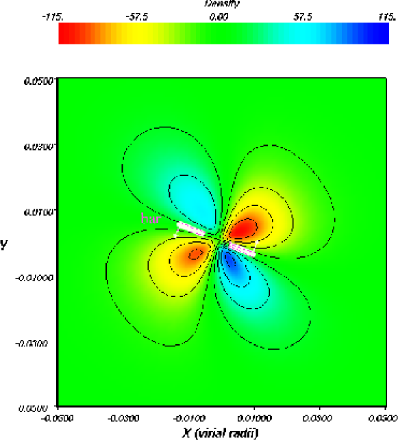
Figure 1: The wake in a halo caused by live disk bar in a live dark-matter halo. The contours and colour mapping show the dark matter wake density in a cut through the disk mid plane from blue (overdense) to red (underdense). The bar position angle is shown in white with the direction of rotation indicated by the arrows. The live disk bar simulations are described in detail in Holley-Bockelmann et al. (2005).

In the first point of view, the bar excites a wake in the halo. An example of such a wake in a self-consistent bar simulation is shown in Figure 1. The excited dark matter halo wake lags the bar, which causes a torque on the bar and removes angular momentum. Naively one might expect the wake to be symmetric about the bar. An explanation for the lag requires us to consider the second point of view: the response of individual orbits. The basic physical picture was outlined in §1: an arbitrary orbit has apsides that precess either forward or backward in the rotating bar frame, depending on the orbit’s energy and angular momentum. A forward-precessing case is shown in the first panel of Figure 2. Over short periods of time, the orbit may torque the bar and later the bar may torque the orbit. However, if we look at this orbit averaged over some time interval $T$, long compared to both its orbital and precession periods, the bar will see an axisymmetric ring of mass density. Such an orbit, therefore, does not change its angular momentum and presents no net torque on the bar. However, there will always be some orbits that are very nearly closed in the bar frame; these are the commensurate or resonant orbits. Near commensurabilities, the precession appears to stop or slow down so much that it might as well be stopped. More precisely, for some fixed time interval $T$, the precession rate is sufficiently slow that density of the orbit averaged over the available time is not axisymmetric. This situation is shown in Panels (b) and (c) of Figure 2 for orbits successively closer to resonance. Resonant orbits feel a coherent forcing at the same phase over many periods. For these orbits, adiabatic invariance is broken and the actions can change. Therefore, the orbit can exchange angular momentum with the bar, which causes both the bar and orbit to evolve.

Figure 2 shows an orbit with prograde procession, but there also exists a corresponding orbit with retrograde procession at a slightly different (in this case larger) energy. To lowest order, these orbits cancel and there is no evolution. Although the net torque from the appropriately chosen pair may cancel, the phase-space density will usually vary with energy and hence the average over phase space will not generally cancel: there will either be more prograde or retrograde orbits. More precisely, the net torque caused by a particular resonance will depend on the gradient of the phase-space distribution function at that resonance (LBK, TW). At any one time, halo orbits are gaining and losing angular momentum owing to all the resonances but the actual net torque occurs as these first order effects cancel. If there were no phase-space density gradient near the resonance, in many cases there would be no evolution. In addition, this net torque imposes a direction to the evolution and the broken symmetry causes the response to either lag or lead the bar position angle. For a given bar perturbation, the response of the halo and, therefore, the net torque on the bar will depend on the phase-space structure of the dark halo.

From the point of view of an individual orbit, the bar induces a periodic distortion in its trajectory, analogous to the modulation of a pendulum by a sinusoidal force. Averaged over an ensemble of orbits with different phases, the sinusoidal response cancels. However, orbits that pass through resonance receive a permanent change that is proportional to the amplitude of the perturbation. The ongoing secular evolution changes both the properties of the bar and the halo. Therefore, the position of the resonance, defined by the closed non-precessing orbit, slowly drifts through phase space (see §3.3). Hence, the time spent by any orbit near a resonance is finite because the entire system evolves as a consequence of the torque applied to these commensurate orbits (TW). If the secular evolution is rapid, the change in energy and angular momentum (or actions) caused by a particular resonance is usually small for any orbit (Weinberg, 1985). The net change for these orbits do not cancel since there are always some measure of orbits close enough to being closed such that the first-order response does not cover all phases. The net angular momentum change then results from the coherent interaction between the forced excitation of the orbit and the slowly changing forcing potential, making the magnitude of the response second-order in the bar perturbation amplitude. In summary, the net torque is proportional both to the phase space gradient of the unperturbed phase space distribution and to the amplitude of the changes in the angular momenta of individual orbits, which is proportional to the square of the perturbation amplitude. If the secular evolution is slower, orbits may linger near the resonance. In this case, the interaction is nonlinear and no longer depends on cancellation or the gradient of the phase-space density. The change in angular momentum for these interactions depends on the square root of the perturbation amplitude (TW). We will see that this regime is important for the ILR. Altogether the overall evolution of the galaxy is driven by the net torque from all the resonances and affects a significant fraction of all orbits. Note that the evolution of the galaxy halo is not caused by a dynamical instability but is secular since it is driven by the exchange of angular momentum with the disk bar.

A common misconception is that resonances are extremely “thin” and, therefore, will only affect a set of orbits of measure zero. Based on the physical explanation above, this statement is incorrect for several reasons. First, one must be careful to distinguish between the width of the resonance in phase space and the width of the resonance in frequency space. The width in phase space depends on the integers defining the commensurability, the amplitude of the perturbation and the frequency of the perturbation, $\Omega_{p}$. The resonance width scales as the square root of the bar amplitude and inversely with the second partial with respect to the resonant action (see eq. 40 and associated discussion). The sign and magnitude of the torque depends on the phase of the apoapse as it passes through the resonance and the net torque results from the sum over all possible phases. If there were insufficient orbital density in a resonance width then one would not get the ensemble result but the contributions from a few orbits at arbitrary phase, which would give a larger, fluctuating contribution. This leads to an important particle number criterion (§3.3).

Secondly, for a real stellar system, the frequency spectrum of the perturbation is not made of sharp lines but is broadened both by the finite age of the galaxy and by the time-dependence of the driving bar perturbation. This is related to our consideration of finite time intervals $T$ in the previous discussion. As long as the integral under each “line” in the spectrum is approximately the same, the time-asymptotic result from secular perturbation theory remains valid. In other words, nearly the same results obtain as long as the resonances are not overlapping, which is true unless the bar slows is so quickly that distinct resonances disappear, which we will demonstrate does not occur in practise. This approximation also breaks down if the overall evolution of the bar pattern speed or the density profiles is so slow that the changes in the individual orbits near the resonance receive nonlinear perturbations. This situation can occur for some resonances even when the bar pattern speed changes rapidly as the bar loses angular momentum (Debattista & Sellwood, 1998; Athanassoula, 2003). In these cases, the perturbation equations may be solved directly, as we will describe below. Even if the bar pattern speed did not change or were held fixed artificially, new orbits would still be affected as the phase-space structure of the system itself evolved. The orbits at or near the resonance will change their actions and will, therefore, occupy a different part of phase-space. This in turn causes the halo potential to change and reach a new equilibrium, moving fresh material into the resonance.

Finally, even in the extremely artificial situation where both the background potential and the bar pattern speed were held fixed, a significant number of orbits would still be affected as long as the system only existed for a finite time. Orbits near a resonance precess away from the resonance but they only do so very slowly: the closer they are to the resonance, the slower their precession. Given an infinite time such orbits would precess through all angles and give an axisymmetric time averaged orbit that would feel no net torque from the bar. In such an eternal system, the orbits affected would be a set a measure zero. However, any astrophysical system only exists for a finite time so the bar changes the actions of many orbits. We explicitly compute the extent in phase space of resonances for finite time perturbations in §3.

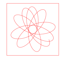
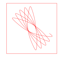
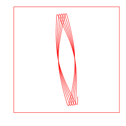
Figure 2: Orbit trajectories viewed the in the frame of a rotating bar. An orbit far from a resonance has the standard “rosette” appearance (Panel A, left). An orbit near a resonance, in this case a 1:2 resonance, has slowly precessing apsides (Panel B, centre). The precession rate decreases as the resonance is approached (Panel C, right). An orbit at resonance is closed.

These same arguments imply that there is no evolution without resonances for a collisionless system in a near-equilibrium state. In the case of a rotating bar, for some fixed $T\gg t_{dyn}$, the density of a time-averaged orbit sufficiently far from a resonance is axisymmetric (see Fig. 2, first panel) and, therefore, applies no torque. In the absence of all resonances, the conserved actions, energy and angular momentum, are preserved for all time in an axisymmetric collisionless stellar system. In this sense, post-formation near-equilibrium galaxy evolution is governed by the resonant transfer of angular momentum. Resonances are not the exception but are required for galaxy evolution! For example, global “modes”, i.e. a density wave that self-similarly evolves and whose ensemble describes all possible excitations such as spiral arms, bars, and halo modes, must dominate angular momentum transfer in the absence of strong non-equilibrium perturbations such as mergers. In the absence of these “modes”, secular evolution can only occur by local collisional scattering, as in an accretion disk, but this process has a characteristic time scale much longer than a Hubble time in galaxies with the observed amount of substructure.

2.1 Hamiltonian perturbation theory

In this and the next several subsections, we convert this physical picture to rigorous criteria for computing resonance phenomena in particle simulations. In later sections and in Paper II, we will explore these dynamics in N-body simulations directly.

One can estimate the overall torque applied by a bar analytically by summing the change in the action caused by the perturbation after some period $T\gg t_{dyn}$ for each orbit in an ensemble using the collisionless Boltzmann equation (CBE). Although more difficult, this approach does the averaging analytically. However, one must be careful to treat the formal divergences that occur at resonances. These divergences are caused by the infinitely large amplitude achieved by an infinitesimal number of particles, but are not a cause for physical concern. Alternatively, one may solve the perturbation theory equations directly (see §2.2). One must also take care to include all the important resonances in this sum including those associated with both discrete and continuous modes. This is a straightforward if somewhat complicated calculation if both self gravity and modes are excluded, which we do here. However, self-gravity can enhance the response at large global scales (Weinberg, 1998a) and is also responsible for the existence of weakly damped discrete modes (Weinberg, 1994), such as the $m=1$ sloshing mode. These modes persist for astronomically relevant time scales and some are sufficiently long-lived that they must be included to follow the dynamics correctly. Real astrophysical systems are not eternal and damped modes are observationally evident in asymmetries (e.g. Vesperini & Weinberg, 2000). With additional work, self gravity and point modes can be accommodated by analytic perturbation theory, although analytic estimates of complex realistic scenarios are difficult. (In §2.3, we present a direct solution to the perturbation theory problem that circumvents all of these difficulties at the expense of CPU time.) We begin by presenting the solution of the CBE both to make contact with previous work (e.g. LBK & TW) and illustrate the difficulties. This development also includes all of the background needed for direct solution.

The torque on the halo may be computed analytically by expanding the rotating bar potential in a Fourier series, where each angle corresponds to a quasi-periodic degree of freedom for an orbit. In a spherical system, one degree of freedom corresponds to radial motion, one to azimuthal motion in the orbital plane, and one to the orientation of the orbital plane. This last angle has zero frequency. The coefficients of the expansion will then depend only on actions ${\bf I}$:

$$H_{1}({\bf r},t)=\sum_{l_{1},l_{2},l_{3}=-\infty}^{\infty}H_{1\,{\bf l}}({\bf I})e^{i(l_{1}w_{1}+l_{2}w_{2}+l_{3}w_{3}-m\Omega_{p}t)}$$ (2)

where $\Omega_{p}$ is the bar pattern speed, $m$ is azimuthal wave number defined by the spherical harmonic $Y_{lm}$, ${\bf I}=(I_{1},I_{2},I_{3})$ are the actions with their corresponding angles ${\bf w}=(w_{1},w_{2},w_{3})$, and ${\bf l}=(l_{1},l_{2},l_{3})$ is an integer vector describing each term in the Fourier series. We will use subscripts ’0’ and ’1’ to denote terms that are zero- and first-order in the perturbation amplitude. The perturbed Hamiltonian includes both the imposed gravitational potential of the bar and the gravitational potential resulting from the response of the halo. These actions follow naturally from Hamilton-Jacobi theory; $I_{1}$, can be immediately identified with the radial action $I_{r}$, $I_{2}$ with the angular momentum in the orbital plane $J$ and $I_{3}$ with the projection of the angular momentum along the $z$ axis $J_{z}$ (e.g. Goldstein, 1950). From Hamilton’s equations, we can obtain the frequency of the angles: $\Omega_{j}=\partial H_{0}/\partial I_{j}$. The subscripted $H_{1\,{\bf l}}$ denotes a coefficient in the action-angle series.

2.2 Solving the perturbation theory

2.2.1 Canonical transformation to slow and fast variables

The natural decomposition of phase space into resonant variables follows from an action-angle transform of the collisionless Boltzmann equation (CBE) in phase space and a Laplace transform in time (e.g. Weinberg, 1998b). To solve for the response, we begin with the linearised CBE:

$${\partial f_{1}\over\partial t}+{\partial H_{0}\over\partial{\bf I}}\cdot{\partial f_{1}\over\partial{\bf w}}-{\partial H_{1}\over\partial{\bf w}}\cdot{\partial f_{0}\over\partial{\bf I}}=0.$$ (3)

The quantities $f_{0}$ and $H_{0}$ are the unperturbed phase space distribution function and the unperturbed Hamiltonian and $f_{1}$ and $H_{1}$ are the first-order terms. The Fourier-Laplace transform of the CBE is

$$s{\tilde{f}}_{\bf l}+i{\bf l}\cdot{\bf\Omega}{\tilde{f}}_{\bf l}-i{\bf l}\cdot{\partial f_{o}\over\partial{\bf I}}{{\tilde{H}}_{1\,{\bf l}}}=0$$ (4)

where $s$ is the Laplace transform variable, the tilde indicates a Laplace transformed quantity, the subscript ${\bf l}=(l_{1},l_{2},l_{3})$ indicates an action-angle transformed variable and ${\bf\Omega}=\partial H_{o}/\partial{\bf I}$. Remember that the total perturbing potential $H_{1}$ is the response combined with the external perturbation. The solution is the inverse Laplace transform of the series:

$$f_{1}(s)=\sum_{l_{1},l_{2},l_{3}=-\infty}^{\infty}{\tilde{f}}_{\bf l}({\bf I},s)e^{i(l_{1}w_{1}+l_{2}w_{2}+l_{3}w_{3})}$$ (5)

where ${\bf w}$ are the three angle variables and ${\bf I}$ are the three action variables.

Each term in the solution described by equation (5) is oscillatory, proportional to $\exp(i{\bf l}\cdot{\bf w})$. For a fixed perturbing frequency $\Omega_{p}$, the inverse Laplace transform couples each term to the perturbing frequency and yields oscillations of the form $\exp[i({\bf l}\cdot{\bf w}-m\Omega_{p}t)]$. For example, assuming an $l=m=2$ quadrupole perturbation as we do for a bar, the integers $(l_{1},l_{2},l_{3})$ take the following values: $l_{1}\in(-\infty,\infty)$, $l_{2}\in{-2,0,2}$ and $l_{3}=2$. Orbits with ${\bf l}\cdot{\bf\Omega}-m\Omega_{p}\rightarrow 0$ define the closed resonant orbits in the frame of reference rotating with the bar. For the parts of phase space very near a resonance described by a particular ${\bf l}=(l_{1},l_{2},l_{3})$, the argument of the exponential will change very slowly for one term and rapidly vary for most of the other terms.

The separation of these characteristic motions is easily performed by making a canonical transformation to two new degrees of freedom where one of the new coordinates corresponds to the angle of the commensurability $w_{s}={\bf l}\cdot{\bf w}-m\phi_{p}(t)$ and

$$\phi_{p}(t)=\int^{t}dt^{\prime}\Omega_{p}(t^{\prime})$$

is the position angle of the perturbation. This can be done with the canonical transformation generating function (e.g. Goldstein Type 2, op. cit.): $F=w_{1}I_{f}+[{\bf l}\cdot{\bf w}-m\phi_{p}(t)]I_{s}$. The new actions and angles are therefore:

$$w_{f} = w_{1}$$ (6)

$$w_{s} = {\bf l}\cdot{\bf w}-m\phi_{p}(t)$$ (7)

$$I_{s} = {1\over l_{2}}I_{2}$$ (8)

$$I_{f} = I_{1}-{l_{1}\over l_{2}}I_{2}$$ (9)

with $H_{new}=H_{old}-m\Omega_{p}I_{s}$ and with $w_{3}$ and $I_{3}$ as before. The angle $w_{s}$ is often called the “slow” angle because its conjugate frequency vanishes at the resonance. There is some arbitrariness in the choice of the “fast” angle, $w_{f}$. For example, the choice $w_{f}=w_{2}$ yields the conjugate actions $I_{s}=I_{1}/l_{1}$ and $I_{f}=I_{2}-l_{2}I_{2}/l_{1}$. This choice might be useful when $l_{2}=0$. In both cases, the angle $w_{s}$ varies very slowly and $w_{f}$ varies rapidly relative to $w_{s}$ near the resonance defined by the vector of integers ${\bf l}$. We can take advantage of this situation by averaging over some time interval $T$ long enough so that all the terms but the resonant one vanish owing to the rapid oscillation in $w_{f}$ but that is small enough so that the argument of the exponent is nearly unchanged. In this way, we reduce the problem to a collection of one-dimensional pendulum equations in $w_{s}$, one for each resonance (e.g. the averaging theorem, Arnold, 1978).

The averaged Hamiltonian in these new coordinates takes the form

$$H(I_{s})=H_{0}(I_{s,r})+{1\over 2}\left.{\partial^{2}H_{0}(I_{s})\over\partial I_{s}^{2}}\right|_{I_{s,r}}(I_{s}-I_{s,r})^{2}+H_{1{\bf l}}\cos w_{s}$$ (11)

where $I_{s,r}$ is the slow action at resonance and $H_{0}$ is the averaged unperturbed Hamiltonian with constant $\Omega_{p}$, up to some arbitrary constant. Equation (11) is a pendulum equation with arm length $M\equiv(\partial^{2}H_{0}(I_{s})/\partial I_{s}^{2})^{-1/2}$ and acceleration $H_{1\,{\bf l}}$. The relative signs for the terms in equation (11) can be arranged by changing the phase of $w_{s}$ as necessary; real positive values are assumed in the square roots of the expressions that follow.

The area defined by the infinite-period trajectory is naturally identified as the width of the particular resonance; this width is proportional to the square root of the Fourier coefficient $H_{1\,{\bf l}}({\bf I})$ from equation (2) (see also eq. 40). A single resonance potential can cover a significant volume in physical space. Individual resonances can overlap in phase space and will lead to chaos and diffusion in the usual way (Chirikov, 1979; Lichtenberg & Lieberman, 1983). However, in galaxy dynamics on large scales, a few low-order resonances often dominate the response in both physical and phase space.

Hamilton’s equations in these new variables with the Hamiltonian from equation (11) explicitly represents the dynamics near resonance. These equations may include an arbitrary time dependence in the perturbation consistent with the averaging. However, these equations only describe a single orbit. A full description of the secular evolution of a galaxy requires the sum of responses over the entire phase space and motivates beginning with equation (3). However, remember that there are astronomical regimes where an orbit may linger close to the resonance making weak nonlinearities important and in these cases we must resort to direct solution over an ensemble of orbits, as we describe below.

The inverse Fourier-Laplace transform of equation (4) is straightforward albeit cumbersome and does not require the equivalent one-dimensional problem explicitly. Having solved for the self-consistent phase-space distribution function for the response, we may then go back to the first order solution of the collisionless Boltzmann equation for the distribution function and integrate over velocities to get the shape of the gravitational potential corresponding to a particular resonance, derive the overall torque, or compute any other phase-space moment of interest. For a given orbit with actions ${\bf I}$, the position ${\bf x}$ determines the angle ${\bf w}$. The integral of ${\tilde{f}}_{\bf l}$ over velocity then requires an implicit solution of the equations defining the angles from positions and momenta. This full, final solution is self-consistent in the limit that the force from the perturbation and the response are small compared to the background restoring force. The result is a second-order perturbation theory calculation. Here, for simplicity, we will eliminate the self consistency by assuming that $H_{1}$ includes only the external perturbation rather than both the external perturbation and the halo response, which is of the same order of magnitude.

As an example of this whole procedure, we sketch the calculation of the response of a homogeneous core to a bar or satellite rotating with frequency $\Omega_{p}$ outside the core. We focus on the ILR, ${\bf l}=(-1,2,2)$, although the basic features of the example apply to any ${\bf l}$. To solve equation (4), we need an expression for $H_{1\,{\bf l}}$. We begin by relating the angle variables to physical quantities. Based on coordinate transformations and geometry, the angle $w_{1}$ describes the radial oscillation of the trajectory, $w_{2}$ describes the azimuthal oscillation of the trajectory, and $w_{3}$ determines the orientation of the orbital plane, which is invariant for a spherical potential. On can express $w_{3}$ in terms of the colatitude $\theta$ of the trajectory and the elevation of the orbital plane $\beta$ (TW). In addition, we find that $l_{2}=-l,-l+2,\ldots,l-2,l$ and $l_{3}=m$ with $l_{1}=-\infty,\ldots,\infty$. The first contributing multipole to the ILR is the quadrupole $l=2,|m|=2$. Furthermore, we can write the perturbing potential as an inner quadrupole $V_{1}(r,\phi,\theta,t)=cY_{lm}(\theta,\phi-\phi_{p}(t))r^{2}$, where $c$ is a constant, because we are considering the perturber to be outside the phase-space region of interest and, since by symmetry $V_{l\,-m}=V_{lm}^{\ast}$, it is sufficient to consider $m=2$ only. With all of these identifications, it is then straightforward to compute the necessary Fourier coefficient:

$$H_{1\,{\bf l}}({\bf I},t)={1\over(2\pi)^{3}}\int\int\int d{\bf w}e^{-i{\bf l}\cdot{\bf w}}cr^{2}({\bf I},{\bf w})Y_{22}(\theta,0)^{im(\phi-\phi_{p}(t))}.$$ (12)

The only explicit time dependence is a pure sinusoidal oscillation so the Laplace transform yields:

$${\tilde{H}}_{1\,{\bf l}}({\bf I},s) = {1\over s+im\Omega_{p}}{1\over(2\pi)^{3}}\int\int\int d{\bf w}e^{-i{\bf l}\cdot{\bf w}}cr^{2}({\bf I},{\bf w})Y_{22}(\theta,0)^{im\phi}$$ (13)

$$\equiv {1\over s+im\Omega_{p}}{\bar{H}}_{1\,{\bf l}}({\bf I})$$

The integrals defining ${\bar{H}}_{1\,{\bf l}}({\bf I})$ can be performed analytically because the motion in a homogeneous core is purely harmonic with constant frequencies throughout the core, but its exact functional form is not important here.

We now substitute equation (13) into equation (4)

$${\tilde{f}}_{1\,{\bf l}}({\bf I},s)=i{\bf l}\cdot{\partial f_{0}\over\partial{\bf I}}{\bar{H}}_{1\,{\bf l}}({\bf I}){1\over s+i{\bf l}\cdot{\bf\Omega}}{1\over s+im\Omega_{p}}$$ (14)

and perform the inverse Laplace transform as follows:

$$f_{1\,{\bf l}}({\bf I},t) = {1\over 2\pi i}\int^{c+i\infty}_{c-i\infty}dse^{st}{\tilde{f}}_{1\,{\bf l}}({\bf I},s)$$ (15)

$$= i{\bf l}\cdot{\partial f_{0}\over\partial{\bf I}}{\bar{H}}_{1\,{\bf l}}({\bf I})\left\{{e^{-i{\bf l}\cdot{\bf\Omega}t}\over i(m\Omega_{p}-{\bf l}\cdot{\bf\Omega})}+{e^{-im\Omega_{p}t}\over i({\bf l}\cdot{\bf\Omega}-m\Omega_{p})}\right\}$$

$$= -{\bf l}\cdot{\partial f_{0}\over\partial{\bf I}}{\bar{H}}_{1\,{\bf l}}({\bf I})e^{-i({\bf l}\cdot{\bf\Omega}+m\Omega_{p})t/2}{\sin[({\bf l}\cdot{\bf\Omega}-m\Omega_{p})t/2]\over({\bf l}\cdot{\bf\Omega}-m\Omega_{p})/2}.$$

This equation has several interesting features. First, the term

$${\sin[({\bf l}\cdot{\bf\Omega}-m\Omega_{p})t/2]\over({\bf l}\cdot{\bf\Omega}-m\Omega_{p})/2}$$

oscillates rapidly and in the limit $t\gg 1/{\bf\Omega}$, $\Omega_{p}$ approaches $\pi\delta({\bf l}\cdot{\bf\Omega}-m\Omega_{p})$. This implies that after a long time, one will only see a contribution for a commensurability ${\bf l}\cdot{\bf\Omega}-m\Omega_{p}=0$. If the satellite or bar was within or nearly within the homogeneous core, $\Omega_{1}\approx\Omega_{2}\approx\Omega_{p}$ and no ILR can possibly exist for small values of ${\bf l}$. A small decrease in $\Omega_{p}$ can remove most of the low-order resonances, and outside of the core, one has $\Omega_{p}\mathrel{\hbox to0.0pt{\lower 3.0pt\hbox{$\mathchar 536\relax$}\hss}\raise 2.0pt\hbox{$\mathchar 316\relax$}}\Omega_{1}\approx\Omega_{2}$ and, therefore, no low-order resonances exist. Second, in a truly homogeneous core, $f_{0}({\bf I})$ is constant so that $\partial f_{0}/\partial{\bf I}=0$ and therefore $f_{1\,{\bf l}}=0$ independent of the resonance ${\bf l}$. These features imply that a bar deep inside of a halo core will have a dramatically reduced torque.

2.2.2 Derivation of first-order changes in angular momentum

We may derive an expression for the change in angular momentum similarly. We begin by deriving the change in angular momentum for a single orbit. The Liouville theorem gives us the rate of change in angular momentum for each orbit as:

$${dL_{z}\over dt}={\partial L_{z}\over\partial t}+[H,L_{z}]$$ (16)

where $[\cdot,\cdot]$ are Poisson brackets (e.g. Goldstein, 1950). Because $L_{z}$ is a conserved quantity in the absence of any perturbation, this equation becomes

$${dL_{z}\over dt}={\partial H\over\partial{\bf I}}\cdot{\partial L_{z}\over\partial{\bf w}}-{\partial H\over\partial{\bf w}}\cdot{\partial L_{z}\over\partial{\bf I}}=-{\partial H_{1}\over\partial w_{3}}$$ (17)

where ${\bf w}$, ${\bf I}$ are action-angle variables and $H_{1}$ is the first-order, perturbed Hamiltonian.

Now expanding $H_{1}$ as an action-angle expansion

$$H_{1}({\bf I},{\bf w},t)=\sum_{\bf l}H_{1\,{\bf l},t}({\bf I})e^{i{\bf l}\cdot{\bf w}},$$ (18)

we can describe the evolution of a particular orbit’s z angular momentum component:

$${dL_{z}\over dt}=-\sum_{\bf l}il_{3}H_{1\,{\bf l}}({\bf I},t)e^{i{\bf l}\cdot{\bf w}}.$$ (19)

We may now integrate over some time interval $T$, defined to be long compared to an orbital time for our orbit with action ${\bf I}$ but short compared to the overall evolutionary time scale. The angles now are explicit functions of time: ${\bf w}(t)={\bf w}_{o}+{\bf\Omega}t$, where ${\bf\Omega}\equiv\partial H_{o}/\partial{\bf I}$ and ${\bf w}_{o}$ is the angle vector at $t=0$. The solution for $L_{z}(t)$ is particularly simple for the sinusoidal time dependence in a simple rotating pattern (e.g. eq. 12). Integrating equation (19), one finds

$$\Delta L_{z}(T) \equiv \int^{T}_{0}dt{dL_{z}\over dt}=-\sum_{\bf l}il_{3}H_{1\,{\bf l}}({\bf I},0)e^{i({\bf l}\cdot{\bf w}_{0})}\left.\left[{e^{i({\bf l}\cdot{\bf\Omega}-m\Omega_{p})t}\over i({\bf l}\cdot{\bf\Omega}-m\Omega_{p})}\right]\right|^{T}_{0}$$ (20)

$$= -\sum_{\bf l}il_{3}H_{1\,{\bf l}}({\bf I},0)e^{i({\bf l}\cdot{\bf w}_{0})}\left\{e^{i({\bf l}\cdot{\bf\Omega}-m\Omega_{p})T/2}{\sin({\bf l}\cdot{\bf\Omega}-m\Omega_{p})T/2\over({\bf l}\cdot{\bf\Omega}-m\Omega_{p})/2}\right\},$$

where we denote $H_{1\,{\bf l}}({\bf I},t)=H_{1\,{\bf l}}({\bf I},0)\exp(-im\Omega_{p}t)$. Equation (20) describes the change in angular momentum $L_{z}$ for a single orbit. To determine the change in angular momentum for a particular portion of phase space, needed to perform a statistical comparison to a N-body simulation, we must average equation (20) over an orbit ensemble. To do this, we multiply equation (20) by the phase-space distribution function $f({\bf I},{\bf w},t)=f_{o}({\bf I})+f_{1}({\bf I},{\bf w},t)$, where $f_{1}({\bf I},{\bf w},t)=\sum_{{\bf l}^{\prime}}f_{{\bf l}^{\prime}}({\bf I},t)e^{i{\bf l}^{p}rimedw}$, and average over the initial phase, $w_{o}$.

There are several subtleties in evaluating the average of equation (20). First, note that the bracketed term on the right-hand side is steeply peaked about ${\bf l}\cdot{\bf\Omega}-m\Omega_{p}=0$ in the limit $T\gg 1/\Omega_{1,2}$; this, of course, owes to the resonance defined by ${\bf l}\cdot{\bf\Omega}-m\Omega_{p}=0$. Second, an average over angles is non-vanishing only for the term $f_{1}$ ($\Delta L_{z}$) when ${\bf l}=-{\bf l}$. This implies that the net torque is second order in $H_{1{\bf l}}$ and this procedure yields a generalised form of the LBK formula (Weinberg, 2004). However, by performing the average over ${\bf w}$, we are implicitly assuming a time interval such that all phases are uniformly represented and this ignores an important feature of the resonance under some circumstances. Recall that near the resonance, we can replace the multidimensional problem with a one-dimensional one in the resonant angle $w_{s}$. Although $w_{1}$ and $w_{2}$ remain distributed in phase, the distribution of $w_{s}$ is correlated by the dynamics of the resonance. To evaluate this average including the correlation, we can replace the integral over phase with an integral over time,

$$\int^{2\pi}_{0}dw_{s}\exp(iw_{s})=\Omega_{s}\int^{T_{s}}_{0}dt\exp(iw_{s}(t))$$ (21)

and evaluate the integral using pendulum dynamics. Far from the resonance, $w_{s}(t)$ will be linear with time. As the orbit approaches the resonance defined by the infinite-period trajectory, the phases will linger near the top pivot point of the pendulum, i.e. an upside down pendulum, and the run of $w_{s}(t)$ will look like stairs with horizontals at $-\pi$ and $\pi$ ($0$ and $2\pi$) if the coefficient of the pendulum potential is negative (positive). Near the infinite-period trajectory, $T_{s}\rightarrow 0$, $\Omega_{s}\rightarrow 0$ with $T_{s}\Omega_{s}\rightarrow 2\pi$. Because the phase will accumulate near the top pivot point in the one-dimensional potential, $\exp(iw_{s})$ will take on the value $1$ or $-1$, again depending on the sign of the resonance potential. Putting this together the phase integral takes the value

$$\int^{2\pi}_{0}dw_{s}\exp(iw_{s})\rightarrow 2\pi\mathop{\rm sign}\nolimits(H_{1{\bf l}})$$ (22)

near the resonance. This bunching and break down of the phase averaging is a consequence of broken adiabatic invariance at the resonance. In the limit of long time intervals, the contributing orbits will be closer and closer to the infinite-period trajectory and, therefore, more and more closely bunched in phase about the top pivot point. Our detailed investigation shows that resonances in astronomically realistic systems can be bunched and require a more subtle treatment than that described here. In particular, one must consider the simultaneous variation of $I_{s}$ with $w_{s}$ and this correlates $H_{1{\bf l}}$ with $w_{s}$. In this case, $\langle\Delta L_{z}(t)\rangle$ scales as $|H_{1{\bf l}}|^{1/2}$ rather than $|H_{1{\bf l}}|^{2}$. TW call the division between these regimes the slow and fast limits and we describe them in the next section. Rather than perform very complicated slow-limit phase averages and time ordering, we will solve the equations of motion by direct numerical integration for an ensemble of orbits.

2.2.3 The slow and fast limits

The rate of secular evolution determines whether or not an orbit lingers near the resonance for many periods or quickly moves through the resonance. The rate of pattern speed evolution characterises the secular change. The natural width in frequency space is the change in the commensurate frequency across the resonant width. The ratio of the rate of pattern speed evolution to the square of the natural width in frequency is a dimensionless ratio that TW call the speed ($s$). In their perturbation calculation, values of $s\ll 1$ give rise to changes in the action that scale as the square root of the perturbation strength and $s\gg 1$ give changes that scale as the square of the perturbation strength. TW call these the slow and fast limits. For a perturbed system whose only time-dependence is its pattern speed, TW defined the quantity speed,

$$s={|m{\dot{\Omega}}_{p}|\over\left|V_{1,{\bf l}}\,{\partial({\bf l}\cdot{\bf\Omega})/\partial I_{s}}\right|}$$ (23)

where $s\gg 1$ is fast and $s\ll 1$ is slow.

For our purposes, these two regimes complicate the perturbation theory but do not result in a dramatic qualitative change in the evolution of a particular orbit. However, the standard perturbation theory (e.g. LBK) assumes the fast limit. A set of exploratory simulations that explicitly tracked $s$ for individual orbits show that the dominant resonances have contributions from the slow limit unless the bar slows down within a rotation period. The ILR is dominated by slow-limit encounters. In practise, we find that $s$ is ${\cal O}(1)$ for most low-order resonances.

2.3 Numerical solution of the the averaged equations: tools and approach

Solving the linearised CBE for arbitrary time dependence in the perturbation and for arbitrary values of the speed $s$ is difficult if not intractable. The added complication of time dependence and contributions from both the slow and fast limits motivates us to abandon explicitly solving the CBE by analytic phase averaging in favour of direct integration of the perturbed Hamiltonian. Averages of phase-space ensembles are then performed by Monte-Carlo integration. Although more CPU intensive, this direct approach to perturbation theory simplifies the complexity of tracking multiple time scales, requires no differentiation between the fast and slow limits, and better facilitates a comparison to N-body simulations. In principle, one can include the self gravity of the response using this method although we do not do so here.

2.3.1 Twist mapping

We can look at the topology and effect of diffusion on the resonant islands by converting the perturbed Hamiltonian near a resonance to a twist mapping applying the now standard procedure (e.g. Lichtenberg & Lieberman, 1983). Begin with the one-dimensional averaged equations,

$$H(I_{s},w_{s})=H_{0}(I_{s})+H_{1{\bf l}}(I_{s})e^{iw_{s}}$$

where $H_{0}$ and $H_{1{\bf l}}$ are the zeroth-order and perturbed parts of the Hamiltonian, respectively. By choosing the phase, with no loss in generality, we may keep only the real part to get

$$H(I_{s},w_{s})=H_{0}(I_{s})+H_{1{\bf l}}(I_{s})\cos(w_{s}).$$ (24)

The surface of section implied by the averaging principle are the successive returns to the $I_{s},w_{s}$ plane separated by time intervals $T_{2}\equiv 2\pi/\Omega_{f}$, where $\Omega_{f}$ is the fast frequency. ¿From Hamilton’s equations, the change in action between two successive periods $T_{2}$ denoted by subscripts $n$ and $n+1$ is

$$I_{s,n+1} = I_{s,n}-\int^{T_{2}}_{0}dt{\partial H_{1{\bf l}}\over\partial w_{s}}(I_{s,n+1},I_{f},w_{s,n}+\Omega_{s,n}t,w_{f}+\Omega_{f,n}t)$$

$$= I_{s,n}-H_{1{\bf l}}({I_{s,n+1}},I_{f})\left[{\sin(w_{s,n}+\Omega_{s,n}T_{2})-\sin(w_{s,n})\over\Omega_{s,n}}\right]$$

where the second equality assumes a simple oscillatory time dependence for the perturbation. To derive a symplectic mapping, we choose a canonical generating function of the form

$$F_{2}=I_{s,n+1}w_{s,n}+2\pi A(I_{s,n+1})+G(I_{s,n+1},w_{s,n}).$$ (26)

The canonical transformation is then:

$$I_{s,n+1} = {\partial F_{2}\over\partial w_{s,n}}=I_{s,n+1}+{\partial G\over\partial w_{s,n}}$$

$$w_{s,n+1} = {\partial F_{2}\over\partial I_{s,n+1}}=w_{s,n}+2\pi\alpha+{\partial G\over\partial I_{s,n+1}}$$ (27)

where $\alpha\equiv dA/dI_{s,n+1}$. Comparing equations (LABEL:eq:twisteqm) and (27) we can deduce that

$$G(I_{s,n+1},w_{s,n})={H_{1{\bf l}}(I_{s,n},I_{f})\over\Omega_{s}(I_{s,n},I_{f})}\left[\cos(w_{s,n})-\cos(w_{s,n}+\Omega_{s,n}T_{2})\right]+h(I_{s,n+1}).$$ (28)

The integration constant $h(I_{s,n+1})$ yields a phase shift that can be absorbed into $\alpha$.

The mapping defined by equations (27) and (28) is well-defined and straightforwardly applied but, for computational speed, the phase-space quantities must be tabled and evaluated using interpolation methods. Truncation error can then lead to an imperfect symplectic mapping, but this situation can be improved as follows. On rearranging terms, equation (27) has the form

$$I_{s,n+1} = I_{s,n}+f(I_{s,n+1},w_{s,n})$$

$$w_{s,n+1} = w_{s,n}+g(I_{s,n+1},w_{s,n}),$$ (29)

which implies that

$$-{\partial g\over\partial w_{s,n}}={\partial f\over\partial I_{s,n+1}}$$ (30)

must hold. The function $g(I_{s,n+1},w_{s,n})$ has only a sinusoidal dependence on $w_{s,n}$ and this implies that the integral in the previous equation can be performed exactly:

$$g(I_{s,n+1},w_{s,n})=-\int dw_{s,n}{\partial g\over\partial w_{s,n}}.$$ (31)

Deriving the mapping in this way, rather than explicitly from equations (26) and (28), guarantees the symplectic condition.

Investigation of the orbit topology for the astronomically-motivated bar perturbation used here shows that most resonances have the standard pendulum topology with one important exception: the relative amplitude of the ILR is sufficiently large that orbit families bifurcate as has been described extensively elsewhere (e.g. Contopoulos & Grosbol, 1989, for a review). This does not present an in-principle problem but, for simplicity, we restrict ourselves to moderate to weak strength bars for comparison between perturbation theory and simulations to remove the complications caused by orbit bifurcation.

The action-angle or Cartesian phase-space coordinates can be obtained at any iteration $n$ (eq. 29) in the twist mapping by another canonical transformation. We apply two-body interactions in the diffusive limit by tabulating the standard orbit averaged diffusion coefficients (Spitzer, 1987). At each step, we transform from slow and fast actions and angles to Cartesian coordinates, apply the change in parallel and perpendicular velocities obtained from a Monte Carlo realization, and then transform back to slow and fast variables.

2.3.2 Numerical solution of the phase-averaged equations of motion

As previously described, the first step in canonical perturbation theory is to expand the phase-space quantities in a Fourier series of actions and angles:

$$\Xi({\bf r},t)=\sum_{l_{1},l_{2},l_{3}}\Xi_{l_{1},l_{2},l_{3}}({\bf I}({\bf r},{\bf v}))e^{i[l_{1}w_{1}({\bf r},{\bf v})+l_{2}w_{2}({\bf r},{\bf v})+l_{3}w_{3}({\bf r},{\bf v})-m\phi(t)]}$$

where we have assumed that the time dependence is periodic with phase angle $\phi(t)$ as previously defined and

$$\Xi_{l_{1},l_{2},l_{3}}({\bf I})=\oint d{\bf w}e^{i(l_{1}w_{1}+l_{2}w_{2}+l_{3}w_{3})}\Xi({\bf r}({\bf I},{\bf r}),t).$$ (32)

If $\Xi$ is a perturbation and we consider Hamilton’s equations, we may transform to new action and angle variables where one angle takes the form

$$w_{s}\equiv l_{1}w_{1}+l_{2}w_{2}+l_{3}w_{3}-m\phi_{p}(t).$$

As long as $|{\dot{w}}_{s}|$ is sufficiently large, the reaction of a orbit to the perturbation will be oscillatory. However, in the limit that

$${\dot{w}}_{s}=l_{1}\Omega_{1}+l_{2}\Omega_{2}+l_{3}\Omega_{3}-m\Omega_{b}(t)\ll\min_{j}(\Omega_{j})$$

the period of the oscillations will be very long and in the limit ${\dot{w}}_{s}\rightarrow 0$ the perturbation may cause a permanent shift in the actions, i.e. a resonance. Near a resonance, the three-degree-of-freedom equations of motion can be transformed to a one-degree-of-freedom problem as described in §2.2.1. The one-dimensional equations of motion take the following form:

$${\dot{w}}_{s} = {\bf l}\cdot{\bf\Omega}-m\Omega_{p}+{\partial W_{l_{1},l_{2},l_{3}}({\bf I})\over\partial I_{s}}e^{iw_{s}}$$

$${\dot{I}}_{s} = -iW_{l_{1},l_{2},l_{3}}({\bf I})$$ (33)

where $W$ is the transform of the perturbation that follows from the application of equation (32)

The validity of the averaging theorem is the only practical limitation in this approximation. It may break down for large amplitude perturbations if resonances overlap (e.g. Chirikov, 1979) or if the system loses or changes equilibrium. The approximation has two important advantages. First, it separates the resonant variable from the others and, thereby, allows the dynamics of the resonance to be isolated from the remaining system, allowing us to check the one-dimensional problem against the full integration of the equations of motion (examples below). Second, because we have averaged over the rapid oscillations, the one-dimensional problem can be solved numerically with a larger time step.

However, unlike the N-body problem, forces in the one-dimensional mapping depend on the velocity, i.e. $\dot{I}_{s}$, and, therefore, we cannot use an explicit symplectic integrator such as Leap Frog. Rather, we use the semi-implicit symplectic RK2 method:

$$q_{n+1}=q_{n}+{\partial H\over\partial p}\left({p_{n}+p_{n+1}\over 2},{q_{n}+q_{n+1}\over 2}\right),$$

$$p_{n+1}=p_{n}-{\partial H\over\partial q}\left({p_{n}+p_{n+1}\over 2},{q_{n}+q_{n+1}\over 2}\right).$$ (34)

We apply this to equation (33) and iterate until it converges using the algorithm:

$$w^{r+1}_{s,n+1} = w^{r}_{s,n}+{\partial H\over\partial I_{s}}\left({w^{r}_{s,n}+p^{r}_{s,n+1}\over 2},{w^{r}_{s,n}+q^{r}_{s,n+1}\over 2}\right),$$

$$I^{r+1}_{s,n+1} = I_{s,n}-{\partial H\over\partial w_{s}}\left({I^{r}_{s,n}+I^{r}_{s,n+1}\over 2},{w^{r}_{s,n}+w^{r}_{s,n+1}\over 2}\right)$$ (35)

where $r=1,2,\ldots$ until $\Delta w_{s}\equiv|w^{r+1}_{s,n+1}-w^{r}_{s,n}|<\epsilon_{1}$ and $\Delta I_{s}|I^{r+1}_{s,n+1}-I^{r}_{s,n}|<\epsilon_{2}$. In practice, this iteration converges for $r\mathrel{\hbox to0.0pt{\lower 3.0pt\hbox{$\mathchar 536\relax$}\hss}\raise 2.0pt\hbox{$\mathchar 316\relax$}}10$ when $\epsilon_{j}=10^{-10}$

2.3.3 Comparison with the direct ODE

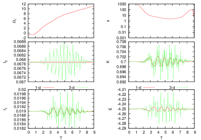
(a) non-resonant

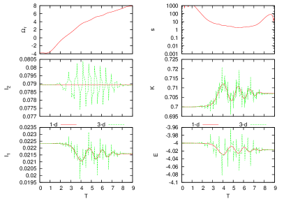
(b) resonant

Figure 3: Panels show the evolution of an orbit during pattern speed evolution of a bar for (a) a non-resonant and (b) a resonant orbit. We plot the actions $I_{1}\&I_{2}$, the energy $E$, the scaled angular momentum $\kappa=J/J_{max}$, the resonance quantity $\Omega_{r}\equiv l_{1}\Omega_{1}+l_{2}\Omega_{2}-2\Omega_{p}(T)$, and the ‘speed’ of the resonance $s$ versus time for the resonance $l_{1}=1$ and $l_{2}=0$ (DRR). The red line shows the one-dimension time averaged solution and the green line the full three-dimensional solution.

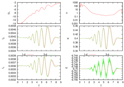
(a) non-resonant

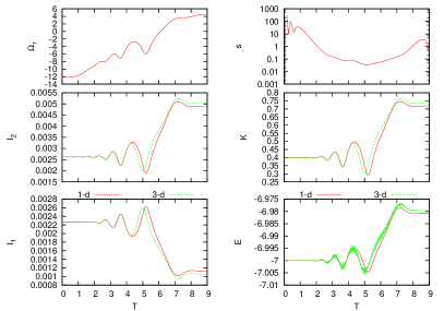
(b) resonant

Figure 4: As in Figure 3 but for the resonance $l_{1}=-1$ and $l_{2}=2$ (ILR).

We want to compare orbit integrations using the time averaged one-dimensional equations with those integrated directly using the three-dimensional equations of motion in the bar quadrupole gravitational potential. For the one-dimensional case, we can perform a canonical transformation to commensurate and non-commensurate action-angle variables and average over the non-commensurate angles, just as in the perturbation theory. For a spherical system, this leaves a reduced, two-degree of freedom problem: one corresponds to the commensurate degree of freedom and one corresponds to the node or angle of ascension of the orbital plane. The conjugate action to this angle is the $z$ component of the angular momentum. The four first-order ordinary differential equations, Hamilton’s equations, can then be integrated as an initial value problem independent of slow or fast limit considerations. For the three-dimensional case, we simply integrate the orbit using the combined halo and quadrupole bar potential using the quadrupole component of the bar perturbation as described in §A.

We assume an NFW dark matter halo and the bar length is the NFW halo scale length $r_{s}$. We impose a time-dependent pattern speed from an N-body simulation with a slowing bar that has a mass that is 1% of the enclosed dark-matter halo mass within the bar radius, which has a 2% force perturbation at maximum. We choose such a weak perturbation to make sure that the perturbation remains only weakly nonlinear in the slow limit, where the strength scales as $|H_{1{\bf l}}|^{1/2}$. We use a standard Leap Frog algorithm for the direct solution of Hamilton’s equations in Cartesian coordinates and use the implicit symplectic algorithm to evolve the averaged equations (described in §2.3.2). Because in the averaged equations the fast oscillatory motion has been removed near the resonance, the time step can be 100 times larger than for the ordinary Cartesian evolution. At each time step, the Cartesian phase space is transformed to the new variables for comparison in the figures.

Figures 3 and 4 compares resonant and non-resonant orbits for the $l_{1}=1,l_{2}=0$ and the $l_{1}=-1,l_{2}=2$ (ILR) resonances integrated using the time averaged one-dimensional perturbation theory and by directly integrating the full three-dimensional equations of motion. The $l_{1}=1,l_{2}=0$ resonant orbit returns to apocenter twice during each bar period. To simplify the discussion, we will call this the direct radial resonance (DRR). An equilibrium phase-space distribution in a spherical halo may be described by two conserved quantities. For convenience we will use the energy $E$ and the angular momentum scaled to the maximum for a given energy $\kappa\equiv J/J_{max}(E)\in[0,1]$.

For DRR (Fig. 3), the fast variable is $w_{2}$ and, therefore, $I_{2}$ is conserved through the resonance as seen for the one-dimensional averaged orbit. The full three-dimensional problem exhibits an oscillation in $I_{2}$ but there is no net change. Outside of resonance, slower modulations by the resonance are seen in both the three-dimensional and one-dimensional solutions for $I_{1}$. The rapid oscillation from the fast degree of freedom is superimposed on this slower motion in the three-dimensional solution. Finally, the net change $I_{s}=I_{1}$ is zero for the non-resonant orbit and non-zero for the resonant orbit.

The overall behaviour for the ILR (Fig. 4) resonance is similar although both $I_{1}$ and $I_{2}$ now both change owing to resonance passage. Note that both the ILR and DDR transitions are not fully in the slow or fast regime. Remember that convenient analytic approximations only exist for $s\ll 1$ (slow) or $s\gg 1$ (fast) and encounters with $s\approx 1$, like these, cannot be solved accurately by analytic perturbation theory but require a numerical solution of the one-dimensional equations of motion.

2.3.4 Comparison of one- and three-dimensional orbit integrations for a phase-space ensemble

In this section, we compare the net changes in the halo phase space caused by the rotating bar using both perturbation theory and the full equations of motion. The latter is performed using an N-body code with a fixed halo potential. We begin with a Monte-Carlo generated phase space for the equilibrium distribution in Cartesian space: $x,y,z,u,v,w$ and for each particle we perform the same orbit calculations described in §2.3.3. The bar mass and length and dark matter halo are as described in the previous section. However, now the evolution of the bar pattern speed is determined by conservation of the total angular momentum in the three-dimensional calculation. The pattern speed for this weak bar slows by 3% during the evolution. The bar amplitude is slowly turned on and then turned off to avoid transients. Transients will not affect the total torque significantly but may produce difficult to interpret phase-space features. The evolution of the bar pattern speed with time is used as an input to the one-dimensional experiment.

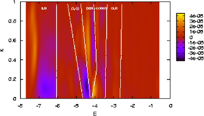
(a) 1-d

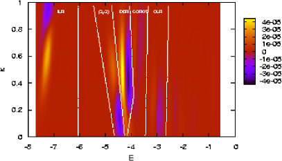
(b) 3-d

Figure 5: Distribution of changes in $L_{z}$ in phase space using the one-dimensional (a) and three-dimensional (b) equations of motion.

In Figure 5, we show the ensemble change in the $z$ component of the angular momentum $\Delta L_{z}$ during the bar evolution. These figures are made by first computing $\Delta L_{z}$ for each orbit as a function of its initial values of $E$ and $\kappa$. We then use kernel density estimation with cross validation (Silverman, 1986) to estimate the smoothing kernel. We increase and decrease this estimate to ensure that the resulting density field is not over smoothed. Using this procedure, Figure 5 compares the change in the $z$ component of the angular momentum after evolving the phase space with the one-dimensional and three-dimensional equations of motion. In the one dimensional case, each resonance must be computed separately and we use the following five resonances (listed in order of their appearance in Figure 5): $(l_{1},l_{2})=(-1,2)$ (ILR), $(2,-2)$, $(1,0)$ (DRR), $(0,2)$ (corotation) and $(1,2)$ (outer Lindblad). Figure 5a is the sum of the five separate one-dimensional phase space calculations.

The low-order resonances with energies larger than -5 agree within 20% for the two cases. However, the ILR ($E\mathrel{\hbox to0.0pt{\lower 3.0pt\hbox{$\mathchar 536\relax$}\hss}\raise 2.0pt\hbox{$\mathchar 316\relax$}}-6$) appears at a somewhat different location and magnitude in the two panels of Figure 5. Because the rate of pattern speed change is so slow for such a weak bar, the orbits linger near the ILR and become nonlinear. A similar experiment with the same parameters but a with a 10 times more massive bar has the opposite problem: the pattern speed decreases by 50% so the orbits are less likely to linger but the overall amplitude is sufficiently high that the interaction itself is nonlinear. As in Figure 5, the resonances at $E>-5$ agree but the one-dimensional integration predicts more torque at ILR than the three-dimensional integration. We also tried using the 1% bar but artificially forcing the bar pattern speed to decrease at the rate of the 10% bar, which resulted in good agreement between the two calculations at ILR.

3 Simulating galaxies with resonances using N bodies

3.1 Description of physical and numerical artifacts

Because Hamiltonian perturbation theory is impractical for complicated astronomical problems and inappropriate for large perturbations such as major mergers, in the end one must “throw caution to the wind” and resort to exploring the dynamics using N-body simulations. Using the development from §2.1, we can derive the requirements necessary to correctly simulate resonance dynamics. There are three requirements on the particle number. First, we require a sufficient number of particles near the resonance to produce the first-order cancellation demanded by the second-order perturbation mechanism (Criterion 1). If you like, an N-body simulation does the phase averaging by Monte-Carlo integration and this criterion ensures convergence of this integral. Second, there must be enough particles so that the time for an orbit to artificially diffuse across the resonance is long compared to the characteristic time scale of a closed orbit in the resonance potential. We separately consider two regimes. Artificial non-astronomical diffusion is caused by small scale graininess in the potential owing to the gravitational force from individual particles (Criterion 2). Similarly, artificial diffusion can be caused by potential fluctuations from Poisson noise at large spatial scales (Criterion 3). In addition, Criterion 3 can describe true astronomical noise. Numerical integration errors can also give rise to a similar diffusion, and hence the integration must be performed accurately.

There is a final criterion that does not depend explicitly on particle number: the potential solver must be able to resolve scales smaller than the resonance potential (Criterion 0) and, of course, the realized phase-space distribution must cover this region. Clearly, this criterion must be satisfied by construction given the resonance potential from equation (2) for the set of desired resonances described by ${\bf l}$ and $\Omega_{p}$.

We investigate each of these issues using the perturbation theory developed in §2.2 to estimate the particle number criteria in §3.2, derive scaling formula in §3.3 and then calibrate these against N-body simulations in §3.4.

3.2 Using perturbation theory to investigate particle number requirements

3.2.1 Coverage

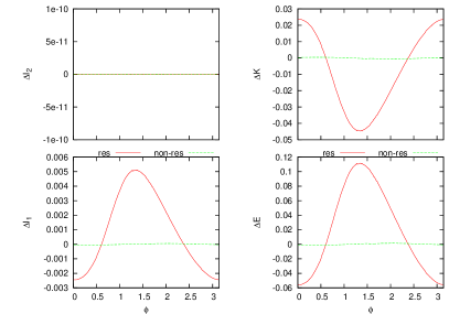
(a) $l_{1}=1,l_{2}=0$

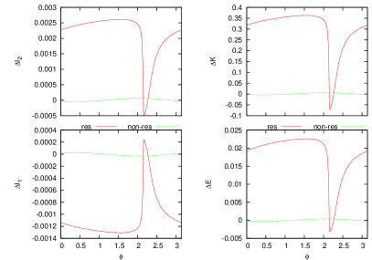
(b) $l_{1}=-1,l_{2}=2$

Figure 6: Variation in conserved-quantity change with bar phase $\phi$ after evolution in pattern speed for the same orbits shown in Figures 3 and 4. The red line is the resonant orbit and the green line is the non-resonant orbit.

The change in the actions $I_{1}$ and $I_{2}$ as a function of bar phase $\phi$ for an ensemble of orbits starting with fixed actions (e.g. energy, angular momentum, and plane inclination) is shown in Figure 6 for DRR and ILR. $E$ and $\kappa$ show a non-sinusoid variation with initial bar phase $\phi$ for orbits that pass through resonance. Orbits gain or lose angular momentum and energy depending on the bar phase at resonance. If one averages over all the phases there is a net change, as expected. There is also a small purely sinusoidal modulation in these quantities for the non-resonant orbits owing to the rotating bar perturbation, which is only barely perceptible in these figures.

This example further illustrates the brief statement in §3.1 that a simulation must have sufficient particles to cover all the phases shown in Figure 6 or one will not get the correct ensemble average. The two resonances are excited by the same bar perturbation but the relative amplitude is much larger for ILR than for DRR giving ILR a peakier profile. The peaky profile requires fewer particles to converge to the mean than the only slightly asymmetric DRR. However, the required particle number may still need to be high to cover ILR adequately owing to the small total mass at low energies. Clearly, the coverage criterion depends on the perturbation amplitude of each resonance separately.

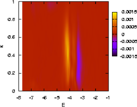
(a) $N=10^{7}$, DRR (1,0)

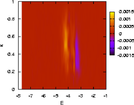
(b) $N=10^{6}$, DRR (1,0)

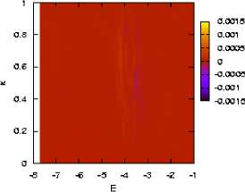
(c) $N=3\times 10^{5}$, DRR (1,0)

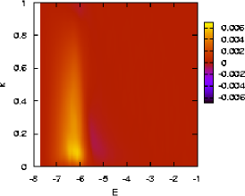
(d) $N=6\times 10^{7}$,ILR (-1,2)

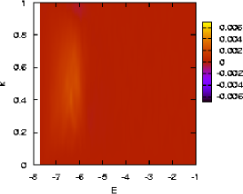
(e) $N=6\times 10^{6}$,ILR (-1,2)

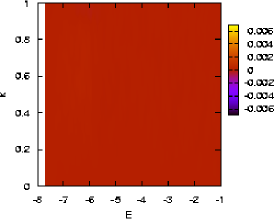
(f) $N=1.8\times 10^{6}$, ILR (-1,2)

Figure 7: Distribution of change in the $z$ component of angular momentum for a full phase ensemble about the orbits described in Figure 6.

In addition, the orbits in Figure 6 have identical initial inclinations near the peak of the contribution for a given energy $E$ and total angular momentum $J$. The full ensemble in an N-body simulation will sample all inclinations and further dilute the net signal from the resonance. One can see the full phase space ensemble result about the initial orbit in Figure 7 where we plot $\Delta L_{z}$ as a function of initial phase space coordinate ($E$,$\kappa$) as in Figure 5. The particle number was increased for both resonances until the amplitude and location of the resonance features in the $E$–$\kappa$ plane remained unchanged. If we decrease the number of particles below this value, the sampling is insufficient in the vicinity of the resonance to recover the full amplitude of the resonance. More than $10^{6}$ ($6\times 10^{6}$) equal mass particles within the virial radius are needed for the DRR (ILR) resonance. Note that we have chosen a very large bar length to reduce the required number of particles. We will see in §3.4 that ILR for a typical strength scale-length sized bar requires $>10^{8}$ particles!

3.2.2 Diffusion

We investigate the effects of two-body perturbations on an orbit near resonance by combining the twist mapping, the solutions to the one-dimensional, and the three-dimensional equations of motion with a Monte-Carlo simulation of the Fokker-Planck equation. The diffusion coefficients are derived from the isotropic phase-space distribution for a spherical equilibrium using the standard prescription (e.g. Spitzer, 1987; Binney & Tremaine, 1987):

$$\delta v_{\parallel} = \langle\Delta v_{\parallel}\rangle\delta T+{\cal R}_{1}(\langle\Delta v_{\parallel}^{2}\rangle\delta T)^{1/2}$$

$$\delta v_{\perp\,1} = {\cal R}_{2}(\langle\Delta v_{\perp}^{2}\rangle\delta T)^{1/2}\cos(2\pi{\cal R}_{3})$$

$$\delta v_{\perp\,2} = {\cal R}_{2}(\langle\Delta v_{\perp}^{2}\rangle\delta T)^{1/2}\sin(2\pi{\cal R}_{3})$$ (36)

where $\delta T$ is the time step, ${\cal R}_{1}$ and ${\cal R}_{2}$ are unit-variance zero-mean normally distributed random variates and ${\cal R}_{3}$ is a random variate uniformly distributed in the unit interval. We adopt a constant value of $\ln\Lambda$ with $\Lambda=b_{max}/b_{min}=1/0.003$. This conservative value is smaller than that of state-of-the-art $\Lambda$CDM simulations and corresponds to a gravitational softening length of about 0.3% of the virial radius. The reader may scale the values of the particle mass $m$ for any value of $\ln\Lambda$ by keeping the product $m\ln\lambda$ fixed. The algorithm for applying equation (36) is as follows: (1) at the end of every twist-mapping iteration or every time step for the symplectic integration of the one-dimensional average equations, we transform the action-angle variables to Cartesian coordinates; (2) equation (36) is applied to the velocities; and (3) the Cartesian coordinates are transformed back to actions and angles.

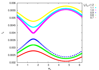
(a) No diffusion

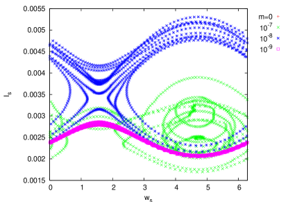
(b) With diffusion

Figure 8: Panel (a) shows orbits on either side of resonance without two-body interactions. The ratio $I_{s}/I_{s}{s,r}$ is the ratio of the initial action to the action of the zero-amplitude homoclinic trajectory. Panel (b) shows the orbit from Panel (a) with $I_{s}/I_{s}{s,r}=0.7$ including two-body interactions for a variety of particle masses $m$.

Figure 8a shows the surface of section of the same orbit near ILR described in the previous figures in the one-dimension slow variables $I_{s}$–$w_{s}$ plane with no small scale diffusion. The bar pattern speed is constant. We label the orbits by $I_{s}/I_{s,r}$ where $I_{s,r}$ is the value of the action at resonance for a zero amplitude bar. Since the amplitude here is not zero, the homoclinic trajectory is offset slightly from $I_{s}=I_{s,r}$. In Figure 8a one can also see how the twist mapping demarcates the expected pendulum topology. Figure 8b begins with the orbit $I_{s}=0.7I_{s,r}$ but adds two-body diffusion corresponding to particle masses of $10^{-7}$, $10^{-8}$, and $10^{-9}$ in units where the total halo mass is unity. For $m=10^{-8}$, diffusion becomes very important and the orbit diffuses to larger $I_{s}$ and even crosses the homoclinic trajectory. For $m=10^{-7}$, the diffusion is so large that the orbit diffuses into the libration zone.

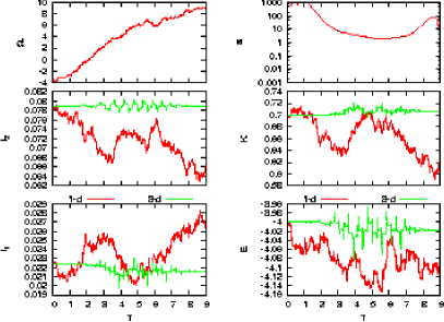
(a) $m=10^{-6}$

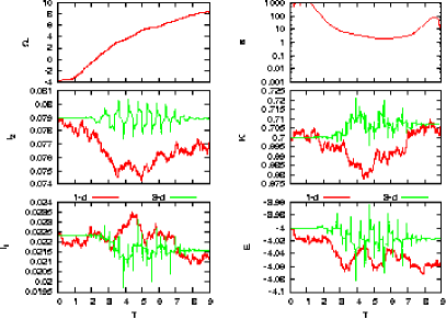
(b) $m=10^{-7}$

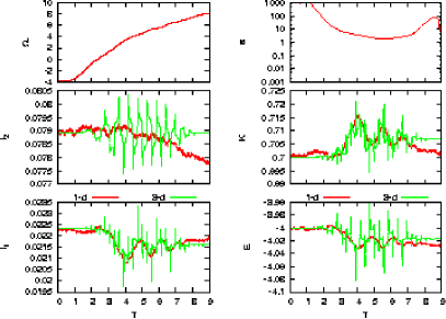
(c) $m=10^{-8}$

Figure 9: As in Figure 3 (DDR) but including two-body diffusion for the particle masses indicated in units of the total mass.

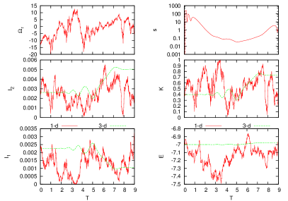
(a) $m=10^{-6}$

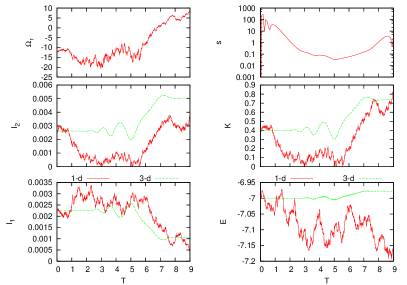
(b) $m=10^{-7}$

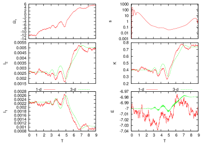
(c) $m=10^{-8}$

Figure 10: As in Figure 9 (ILR) but for the orbit in Figure 4.

Similarly, we may solve the one-dimensional equations of motion including the two-body diffusion for the same test orbits shown in Figures 3 and 4; these are shown in Figures 9 and 10, respectively, for particle masses of $m=10^{-6}$, $10^{-7}$, and $10^{-8}$. The two-body fluctuations are only included in the one-dimensional solution, the three-dimensional solution is left unchanged for comparison. Only at $m=10^{-8}$ does the two-body perturbed solution begin to follow the unperturbed solution. This is consistent with our twist mapping results. In short, values of $m$ equal to or smaller than those of typical N-body simulations destroy resonances.

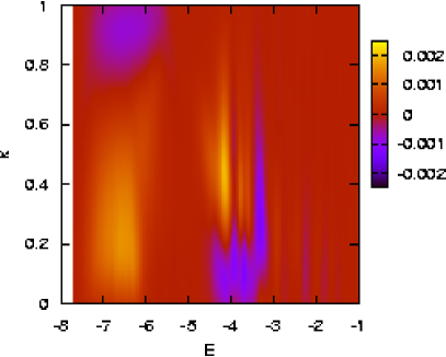
(a) $m=0$

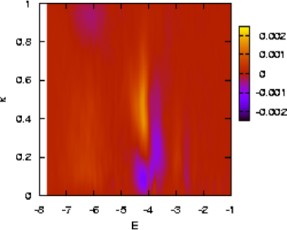
(b) $m=10^{-6}$

Figure 11: Distribution of $\Delta L_{z}$ from direct integration results of the three-dimensional equations of motion for an evolving rotating bar without (a) and with (b) two-body diffusion for $m=10^{-6}$.

Figure 11 shows the results of an integration using the three-dimensional equations of motion for an ensemble $6\times 10^{7}$ particles in the quadrupole bar perturbation both without and with two-body diffusion equivalent to $10^{6}$ particles. This isolates the effects of diffusion from those of coverage. With two-body diffusion, the inner ILR is significantly reduced. However, the outer low-order resonances, $l_{1}=1,l_{2}=0$ in particular, still appear at their predicted strength and location. How can we understand this in the context of the large changes in orbital structure near resonances we saw in the twist mapping and one-dimensional solutions? Even though the random walk in actions seen in Figures 8, 9 and 10 may be larger than the width of the resonance, the pattern speed of the rotating potential will continue to evolve and sweep past the ‘walking’ orbit at some nearby action whenever $l_{1}\Omega_{r}+l_{2}\Omega_{\phi}=m\Omega_{p}$. At this point, the adiabatic invariant corresponding to the slow motion will break and the orbit will feel a coherent ‘kick’. However, orbit cannot linger near the homoclinic trajectory owing to the random walk and will, therefore, always be in the fast limit. In other words, the two-body noise diffusion of N-body particle-particle simulations, which is much larger than that in true dark matter haloes, is sufficient to cause slow limit transitions to become fast limit transitions.

Note that the speed parameter is fast ($s>1$) for the $l_{1}=1,l_{2}=0$ resonance (DDR) (Fig. 3) but slow ($s<1$) for the ILR (Fig. 4). The clear difference in magnitude between the ILR in the slow limit (Fig. 11a) and when it is forced into the fast limit by noise (Fig. 11b) is a consequence of the smaller changes in angular momentum for a fast-limit encounter. The corotation resonance ($l_{1}=0,l_{2}=2$) appears at $E\approx-3.7$, immediately to the right of the $l_{1}=1,l_{2}=0$ resonance and at lower amplitude. This resonance has $s\approx 1$ and its amplitude is also diminished by the diffusive effects of two-body encounters. Only the amplitude of the DRR is preserved.

3.2.3 Fluctuations on large spatial scales

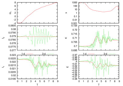
(a) $m=10^{-5}$, DRR (1,0)

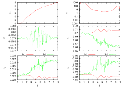
(b) $m=10^{-4}$, DRR (1,0)

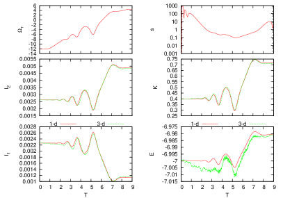
(c) $m=10^{-6}$, ILR (-1,2)

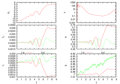
(d) $m=10^{-5}$, ILR (-1,2)

Figure 12: As in Figures 9 and 10 but including diffusion caused by large-scale fluctuations for the particle masses indicated in units of the total mass.

The calculations in the previous section emphasise the fluctuations in the gravitational field dominated by two-body encounters on relatively small scales. Formally, large scale contributions were also included. The contribution to the fluctuations on large scales in the homogeneous approximation leads to a divergence at the upper end of the Coulombic logarithm $\ln\Lambda$. Physically, this divergence is removed by the inhomogeneity of a gravitationally bound galaxy and a realistic estimate must be computed differently. In this section, we explicitly address the role of fluctuations owing to noise at large scales, both in simulations and astronomically owing to dark-matter substructure.

To appreciate the physical situation, consider the forcing of an inner-halo orbit by a disturbance (such as orbiting dark-matter subhaloes) in the outer galaxy. There are two requirements for a distant disturbance to cause an effect on the inner orbit: 1) the force must vary over the region sampled by the orbit, otherwise there can be no work done relative to the background potential; and 2) the time scale of the disturbance must be smaller than one of the orbit’s natural periods, otherwise the motion will be adiabatically invariant. These sorts of considerations are very similar to those important for the bar–halo interaction discussed in §2 and can be approached similarly.

Weinberg (2001) derives a formalism for treating the evolution of orbits including statistical fluctuations caused by perturbers of various sorts. Assuming that the perturbations are a first-order Markovian process, i.e. they do not retain any memory of their prior state, the evolution equation naturally takes the Fokker-Planck form (Pawula, 1967). In particular, Weinberg (2001) works out analytic expressions for the diffusion coefficients and we will use them here. The calculation explicitly includes the spatial and temporal correlations of any physical perturbation. The expression for the coefficients have two parts: 1) a second-order reinforcement by the perturbation on the induced distortion on the orbit, typical of any second-order perturbation theory as described in §2.1; and 2) a correlation coefficient that describes the spatial and temporal correlation of the perturbation. If we denote the change in component $j$ of the action at time $t$ after evolving by a period $\tau$ as $\Delta I_{j}(t+\tau)$, then action-space diffusion coefficients from Weinberg (2001) are:

$$D^{(1)}_{j}({\bf I},t) = \lim_{\tau\rightarrow 0}{\left\langle\Delta I_{j}(t+\tau)\right\rangle\over\tau}$$

$$= -{1\over f_{0}({\bf I})}l_{j}{\bf l}\cdot{\partial f_{o}\over\partial{\bf I}}\left|Y_{ll_{2}}(\pi/2,0)\right|^{2}\sum_{\mu\nu}\sum_{rs}r^{l}_{l_{2}m}(\beta)r^{\ast l}_{l_{2}m}(\beta)W^{l_{1}\,\mu}_{ll_{2}m}({\bf I})W^{\ast l_{1}\,\nu}_{ll_{2}m}({\bf I})\times$$

$$\left\{(2\pi)^{3}\sum_{\bf l}\int d^{3}If_{o}({\bf I})|Y_{ll_{2}}(\pi/2,0)|^{2}r^{l}_{l_{2}m}(\beta)r^{l}_{l_{2}m}(\beta)\times\right.$$

$$\left.W^{l_{1}\,r}_{ll_{2}m}({\bf I})W^{\ast l_{1}\,s}_{ll_{2}m}({\bf I}){\cal M}^{lm}_{\mu r}({\bf l}\cdot{\bf\Omega}({\bf I})){\cal M}^{\ast lm}_{\nu s}({\bf l}\cdot{\bf\Omega}({\bf I}))2\pi\delta\left({\bf l}\cdot{\bf\Omega}({\bf I})\right)\right\},$$

$$D^{(2)}_{jk}({\bf I},t) = \lim_{\tau\rightarrow 0}{\left\langle\Delta I_{j}(t+\tau)\Delta I_{k}(t+\tau)\right\rangle\over 2\tau}$$

$$= {l_{j}l_{k}\over 2}\left|Y_{ll_{2}}(\pi/2,0)\right|^{2}\sum_{\mu\nu}\sum_{rs}r^{l}_{l_{2}m}(\beta)r^{\ast l}_{l_{2}m}(\beta)W^{l_{1}\,\mu}_{ll_{2}m}({\bf I})W^{\ast l_{1}\,\nu}_{ll_{2}m}({\bf I})\times$$

$$\left\{(2\pi)^{3}\sum_{\bf l}\int d^{3}If_{o}({\bf I})|Y_{ll_{2}}(\pi/2,0)|^{2}r^{l}_{l_{2}m}(\beta)r^{l}_{l_{2}m}(\beta)\times\right.$$

$$\left.W^{l_{1}\,r}_{ll_{2}m}({\bf I})W^{\ast l_{1}\,s}_{ll_{2}m}({\bf I}){\cal M}^{lm}_{\mu r}({\bf l}\cdot{\bf\Omega}({\bf I})){\cal M}^{\ast lm}_{\nu s}({\bf l}\cdot{\bf\Omega}({\bf I}))2\pi\delta\left({\bf l}\cdot{\bf\Omega}({\bf I})\right)\right\}.$$

The spatial component of the response is expanded in a orthogonal series, the $r^{l}_{l_{2}m}(\beta)$ rotate the spherical harmonics, and the terms $W^{l_{1}\,r}_{ll_{2}m}$ describe the coefficients of the action-angle expansion for the $r^{th}$ basis function. The operator ${\cal M}^{lm}_{\mu r}(\omega)$ describes the self-gravitating response owing to an applied frequency $\omega$ in the space spanned by the basis. The sums on $\mu,\nu$ and $r,s$ are the sums in the space of this operator. In this study, we will ignore self gravity and hence the ${\cal M}^{lm}_{\mu\nu}$ become identity matrices. The limit $\tau\rightarrow 0$ must be taken in the sense that $\tau$ is small compared to the evolutionary time scale owing to the fluctuations but remains large compared to the dynamical time. The time dependence in the diffusion coefficients reminds us that the underlying equilibrium distribution $f_{o}({\bf I})$ changes on an evolutionary time scale but, for the purposes of the computation, is held fixed on a dynamical time scale. The lowest-order temporal variation has been explicitly removed by the limit $\tau\rightarrow 0$. The integrals may be simplified by noting that $d^{3}I=dEdJJd(\cos\beta)/\Omega_{1}(E,J)$. We can then do the integral in $\beta$ using the orthogonality of the rotation matrices as previously described. For a given equilibrium distribution function $f_{o}({\bf I})$, the term in curly brackets in equations (LABEL:eq:mom1expA) and (LABEL:eq:mom2expA) is the spatial and temporal correlation of the perturbation and need be computed only once since it is independent of the local value of the actions.

We now use equations (LABEL:eq:mom1expA) and (LABEL:eq:mom2expA) to compute the fluctuations by random realisation. The procedure parallels that in §3.2.2: one generates new values of ${\bf I}$ from $D^{(1)}_{j}({\bf I},t)$, $D^{(2)}_{jk}({\bf I},t)$ and Gaussian random variates. Here we do not have the luxury of uncorrelated parallel and perpendicular motion as in the infinite homogeneous case but we must diagonalise $D^{(2)}_{jk}({\bf I},t)$ (e.g. by a Jacobi rotation) to generate uncorrelated random variates in ${\bf I}$.

Figure 12 shows the evolution of an orbit near DRR and ILR perturbed by large-scale fluctuations (cf. Figs. 3 and 4). The particle number requirements are 1000 and 100 times smaller than that for two-body diffusion, respectively, for the two resonances. From the N-body simulation point of view, the two-body relaxation from the previous section sets a minimum particle number in a particle-particle code (e.g. direct, tree, mesh, etc.) and the large-scale fluctuations considered here sets a minimum particle number in an expansion code. By limiting the spatial scales, the expansion-based solver dramatically reduces the relaxation and potentially the particle requirements.

3.2.4 Implications for dark-matter substructure

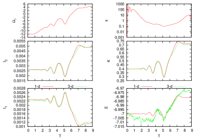
(a) ${\bar{m}}f_{ss}=10^{-5}$

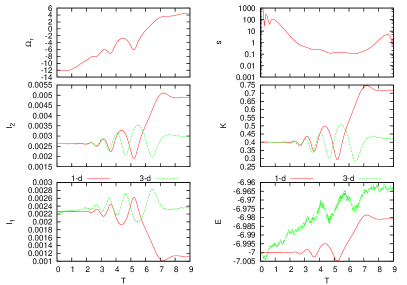
(b) ${\bar{m}}f_{ss}=10^{-4}$

Figure 13: As in Figure 12 for the ILR (-1,2) including the effects of substructure with orbits restricted to $r>r_{s}$.

We can use these results to estimate the importance of astronomical noise sources on bar–halo resonances. In principle, the fluctuations from any physical process can be computed as described in Weinberg (2001). The most common and perhaps relevant noise comes from orbiting substructure. Ignoring orbital decay, the calculation is identical to that discussed in the previous section. $\Lambda$CDM simulations provide both a spatial density distribution and mass function for dark-matter substructure. Oguri & Lee (2004) show that these distributions can be modelled using a Press-Schechter approach (Press & Schechter, 1974) extended to include tidal stripping and orbital decay. Oguri & Lee find that the satellite masses have the cumulative distribution $N(>m)\propto m^{-1}$ for $m/M_{vir}$ from $10^{-6}$ to $0.3$. The spatial distribution of substructure is shallower than the overall dark matter distribution with shallower profiles for larger values of $m$. We will assume, for simplicity, that the maximum substructure mass, $m_{max}/M_{vir}$, is 0.3 and the smallest substructure mass, $m_{min}/M_{vir}$ is $10^{-6}$. This implies that the mean mass (in virial mass units) is

$${\bar{m}}={\log(m_{max}/m_{min})\over\left(1/m_{min}-1/m_{max}\right)}\approx 1.3\times 10^{-5}.$$ (39)

Let the fraction of the dark matter in substructure with $m>m_{min}$ be $f_{ss}$. Then, the diffusion coefficients from equations (LABEL:eq:mom1expA) and (LABEL:eq:mom2expA) for particle mass $m$ may be scaled to $m={\bar{m}}f_{ss}$. Assuming that the fraction of the mass in substructure $f_{ss}\approx 0.1$ (Gao et al., 2004) and using equation (39) we have ${\bar{m}}f_{ss}\approx 10^{-6}$. To implement the effect of tidal stripping, we assume that the density distribution of substructure within the dark halo takes the same NFW form as the dark matter but with no substructure inside of $r_{s}=1/15$ (units $R_{vir}=1$). This requires restricting the phase-space integral inside the curly brackets in both equations to orbits with $r>r_{s}$.

Figure 13 shows the now familiar ILR orbit perturbed by large scale fluctuations from orbiting substructure restricted to orbits with $r>r_{s}$. Now, ${\bar{m}}f_{ss}$ must be larger than about $10^{-5}$ to destroy the resonance, which is an order of magnitude larger than the actual substructure noise.

3.3 Calibration of particle number criteria: scaling formulae

All of the particle number criteria described in §3.2 have natural scalings in terms of physical quantities: properties of the equilibrium gravitational potential and the perturbation such as bar strength, bar shape, bar pattern speed, etc. We derive simple scaling relations in this section and calibrate them using the results of §3.1 and additional simulations.

3.3.1 Method

To calibrate the scaling estimates for the particle number requirements defined in §3.2, we evolve phase-space ensembles as described in §2.3.4. We can use both the one-dimensional and three-dimensional equations of motion to study each of the three criteria from §3.2.

3.3.2 Coverage

The coverage criterion demands that one samples phase space sufficiently densely in the vicinity of a resonance to ensure the correct ensemble average. The resonance potential is defined by the one-dimensional pendulum problem from equation (11) and is simply the Fourier action coefficient corresponding to the commensurability ${\bf l}$. We define the half-width of the resonance potential as the maximum extent of the infinite-period trajectory in the one-dimensional phase space:

$$\delta I_{s}=\sqrt{2M^{2}H_{1\,{\bf l}}}.$$ (40)

This is called the resonance width in the celestial mechanics literature. Hence, we can use perturbation theory to estimate a characteristic width or volume in phase space associated with each resonance. Because it depends on both the Fourier action-angle expansion coefficient and the change in slow frequency with slow action, this width depends on both the order of the resonance and the amplitude of the perturbation.

As the galaxy halo slowly evolves, the resonance defined by the commensurability ${\bf l}\cdot{\bf\Omega}-m\Omega_{p}=0$ sweeps through phase space as described in §2. A secular torque occurs only if there are enough particles so that the first-order sinusoidal oscillations cancel to leave the second-order changes. We, therefore, require sufficient particles, $n_{p}$, in a fraction $\epsilon_{w}$ of the resonance width to obtain a mean cancellation of the first-order forced response. We use the resonance width to estimate the number of particles needed to resolve this phase space volume. The commensurability ${\bf l}\cdot\Omega=m\Omega_{p}$ defines a track in the $E$ and $J$ (or $I_{r}$ and $I_{\phi}$) phase-space plane. The resonance width in equation (40) takes values along this locus. For a spherical isotropic stellar system, most resonance tracks defining the commensurability have only a small variation with $\kappa\equiv J/J_{max}(E)$ for fixed $E$. We optimistically assume that an ensemble average over angles for orbits over a large range in $\kappa$ for the same resonance cancels the first-order oscillation. Clearly more careful approximations that explicitly compute the full phase-space volume for coherent contributions are possible. In addition, we assume that the phase-space distribution is isotropic. The phase-space fraction within an energy width $\Delta E$ for an isotropic phase-space distribution function $f(E)$ is:

$$dF=\int d{\bf w}\,d{\bf I}\,f(E)\delta[E-E({\bf I})]=p(E)f(E)dE=n(E)dE$$ (41)

where

$$p(E)=2(2\pi)^{3}J_{max}^{2}(E)\int^{1}_{0}d\kappa\,\kappa/\Omega_{1}(E,\kappa)$$

with normalisation

$$1=\int dF=\int dEp(E)f(E).$$

We then use the width in $E$, corresponding to $\delta I_{s}$ defined in equation (40), to estimate the fraction of phase space $f_{crit}$ that we require to be populated with at least $n_{p}$ particles as follows:

$$f_{crit} \approx \epsilon_{w}p(E)f(E){\partial E\over\partial I_{s}}(\delta I_{s})$$ (42)

$$= \epsilon_{w}{n(E)({\bf l}\cdot\Omega)\sqrt{2H_{1\,{\bf l}}}\over\left|\partial^{2}H_{0}(I_{s})/\partial I_{s}^{2}\right|^{1/2}_{I_{s,r}}}$$

where ${I_{s,r}}$ is the value of the slow action at the resonance. This expression for $f_{crit}$ is independent of the choice for $w_{f}$, as it must be, but depends of course on the resonance ${\bf l}$.

We can now use $f_{crit}$ to estimate the number of particles needed to resolve a resonance. Explicitly, our requirement $n_{p}\leq Nf_{crit}$ implies that the minimum critical particle number for resonance ${\bf l}$ is $N_{req,{\bf l}}=n_{p}/f_{crit}$. For example, if we demand that $n_{p}=10$ particles should span one tenth of the resonance width for $\epsilon_{w}=0.1$ to obtain good first-order cancellation, we require the simulation to contain the following minimum number of particles:

$$N_{req,{\bf l}}={n_{p}\over\epsilon_{w}}{\left|\partial^{2}H_{0}(I_{s})/\partial I_{s}^{2}\right|^{1/2}\over n(E)({\bf l}\cdot\Omega)\sqrt{2H_{1\,{\bf l}}}}=100{\left|\partial^{2}H_{0}(I_{s})/\partial I_{s}^{2}\right|^{1/2}\over n(E)({\bf l}\cdot\Omega)\sqrt{2H_{1\,{\bf l}}}}.$$ (43)

This factor of 100 is only a crude guess but tests in §3.4 suggest that this is approximately the correct value.

3.3.3 Noise

As we have seen from §3.2.2, fluctuations on very small spatial scales (two-body relaxation) causes diffusion in the conserved quantities of an orbit. Recall that in linear perturbation theory, torque is transferred to orbits whose apses are very slowly precessing in the bar frame. This implies that the orbits must remain quasi-periodic for at least several periods in the bar frame. The period of the slowly precessing orbit is best characterised by the period of the closed resonant orbit. For our spherical system, this period is

$$P_{res}=\max\left({2\pi\over\Omega_{1}}|l_{2}|,{2\pi\over\Omega_{2}}|l_{1}|\right).$$ (44)

We therefore require that the diffusion length in the conserved quantities over some number of $P_{res}$ be smaller than the resonance width. Let the diffusion coefficient, the mean-squared rate of spread of an ensemble of particles in the slow action $I_{s}$, be denoted as $D_{I_{s}I_{s}}$. Using equation (40), we can then express this criterion as

$$\tau\equiv{\epsilon_{r}(\delta I_{s})^{2}\over D_{I_{s}I_{s}}P_{res}}>1$$ (45)

where $1/\epsilon_{r}$ is the desired number of resonance periods over which the orbit must remain stable. We estimate that plausible values of $\epsilon_{r}$ range from 0.1 to 0.3 and use $\epsilon_{r}=0.3$ in the estimates given below. We test this choice in §3.4. For a fixed phase-space distribution with unit mass, the diffusion coefficient scales as the mass per particle or inversely with the number of particles $N$. Now, if we derive $D_{I_{s}I_{s}}$ for a unit-mass particle then the number of particles required to satisfy the criterion in equation (45) is

$$N_{req}=1/\tau={D_{I_{s}I_{s}}|_{{\bar{m}}=1}P_{res}\over\epsilon_{r}(\delta I_{s})^{2}}.$$ (46)

Direct-summation N-body simulations (including tree-algorithm based simulations) follow individual particle motions with a resolution approximately equal to the interparticle softening scale. We express the relaxation present in these codes at small scales using two-body relaxation as in §3.2. The standard expressions are given in terms of energy $E$ and angular momentum $J$. The diffusion coefficient $D_{x_{j}x_{k}}$ transforms to new variables $x^{\prime}_{\mu}=x^{\prime}_{\mu}(\{x_{j}\})$ as

$$D_{x^{\prime}_{\mu},x^{\prime}_{\nu}}=\sum_{jk}{\partial x^{\prime}_{\mu}\over\partial x_{j}}{\partial x^{\prime}_{\nu}\over\partial x_{k}}D_{x_{j}x_{k}}$$ (47)

(e.g. Risken, 1989). Depending on the value of $l_{j}$, we are free to choose either $I_{1}\equiv l_{1}I_{s}$ or $I_{2}\equiv l_{2}I_{s}$. We may then derive $D_{I_{s}I_{s}}$ from the homogeneous diffusion coefficients $D_{E\,E},D_{E\,J},D_{J\,J}$ and equation (47).

In the same way, the large-scale expansion-based diffusion coefficients in equations (45) and (46) together with equation (47) yields $D_{I_{s}I_{s}}$ and particle number criteria for noise on large scales. We use the same expansion from our Poisson solver for the expansion in these diffusion coefficients although any biorthogonal expansion would suffice. This approach also facilitates a direct comparison with the simulations.

3.3.4 Time steps

Comparison between the one- and three-dimensional solutions for individual orbits allows us to investigate the time step criteria necessary to obtain a correct transition through resonance. This is more stringent than the requirement that the energy or actions be conserved for an equilibrium orbit. For an orbit with energy E, we find that a time step with approximately 1/100 of the period of the circular orbit with the same energy is necessary.

3.4 Results

Table 1: Scaling of particle number requirements.

Requirement	Scaling	Description
$N_{req,{\bf l}}$	$M_{p}^{-1/2}$	coverage
$N_{req,Ch}$	$M_{p}^{-1}$	small-scale noise
$N_{req,SCF}$	$M_{p}^{-1}$	large-scale noise

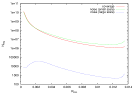
(a) ILR (-1,2)

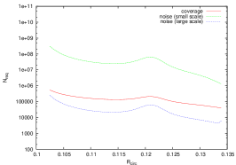
(b) corot (0,2)

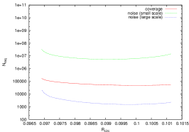
(c) DRR (1,0)

Figure 14: The three particle number criteria—coverage, and small and large scale noise—for the indicated resonances for a large weak bar versus radius.

We can use the formula derived in §3.3 to determine the particle number requirements, i.e. the number of equal mass particles within the virial radius. We start with a halo-scale-length bar, i.e. bar radius $=r_{s}=0.067$, whose mass is 1% of the dark matter mass within that radius and a pattern speed at one-half of its corotation value. We plot the results for each of the three criteria for three of the most important resonances, ILR (-1,2), corotation (0,2), and DRR (1,0) in Figure 14. Table 1 describes how each of these criteria scale with the mass of the perturbing bar, $M_{b}$. We choose such a weak bar to facilitate comparison with perturbation theory but the reader may scale these estimates to any bar mass using these relations. Since both the energy and angular momentum change along the track of each resonance, as seen in previous figures (e.g. Fig. 7), we plot the requirement for each criteria as a function of the radius of a circular orbit with the same energy, $r_{circ}$. For this interaction, the most important resonances are the ILR and DRR. We show the corotation resonance (0,2) for comparison. Note the radial location of the resonances: the corotation resonance and DRR are around the end of the bar, 0.067, while the ILR begins at approximately one quarter of the bar radius, 0.014, and extends inward to very small radii, at least as small as 0.02 times the bar radius. It is important for the Poisson solver to resolve down to this scale, approximately $10^{-3}$ times the virial radius in this case. Hence, in this figure we assume a gravitational softening length of this size when calculating the small-scale noise requirement.

For all resonances, the small-scale noise criteria is the most severe but it is comparable to the coverage criterion for ILR. Remember that, as they are usually used, the small scale noise criterion only applies to particle-particle codes, e.g. direct, tree, and grid based, and not to expansion SCF codes. As described in §3.3.3, small-scale noise will strongly affect which orbits enter resonance and the regime of the resonance. However, coverage will dominate the small-scale noise for a stronger, i.e. more massive, bar at ILR according to the scalings in Table 1. The estimates for coverage are consistent with the convergence of $\Delta L_{z}$ in phase space with particle number for coverage alone computed using one-dimensional averaging as shown in Figure 7. Similarly, comparison of Figure 14 and Figures 9 and 10 show consistency: the scaling relations require more than $10^{7}$ particles for DRR and considerably more for ILR.

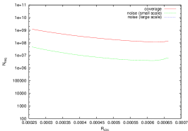
(a) ILR (-1,2)

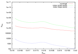
(b) corot (0,2)

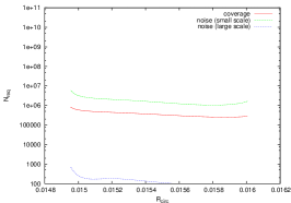
(c) DRR (1,))

Figure 15: The three particle criteria—coverage, and small and large scale noise—for the indicated resonances for a disk-scale-length, moderate strength bar.

Figure 15 shows the same predictions for an approximately scale-length sized moderate strength bar, i.e. bar radius$=r_{s}/6.7=0.01$. The bar mass is 10% of the enclosed dark matter mass, making the maximum relative amplitude of the asymmetric to axisymmetric force 30%. This bar requires a force resolution of $2\times 10^{-4}$ times the virial radius to fully resolve the ILR, which we use in our calculation of the small-scale noise. The coverage criterion demands a very large particle number to correctly couple to the bar–halo ILR: approaching $10^{9}$ particles. The trends for the outer resonances are similar to those for the large bar but the coverage criterion is relatively more important. Approximately $5\times 10^{7}$ particles are needed for these resonances. Because the ILR for a scale-length bar occupies very low energies in the cusp, we can check the criteria in Figure 15a for by realizing only a small subset of the full phase space. By varying the energy range, we may use between $10^{6}$ and $10^{7}$ actual particles to achieve a suite of realizations logarithmically spaced between $10^{6}$ and $10^{9}$ equivalent particle numbers. The ILR resonance only reaches its full amplitude for $N\mathrel{\hbox to0.0pt{\lower 3.0pt\hbox{$\mathchar 536\relax$}\hss}\raise 2.0pt\hbox{$\mathchar 318\relax$}}3\times 10^{8}$ particles consistent with the prediction in Figure 15.

As described in §3.3.3, the diffusion will cause a drift in the orbits that pass through resonance and cause all resonant interactions to be in the fast limit, even if they would be in the slow limit without noise. Therefore, one may relax the small-scale noise criteria if one knows a priori that all resonances are fast and possibly still obtain the correct overall torque. This coincidence explains the convergence of the total torque in simulations that do not meet the small-scale noise criterion. For the bar–halo interaction emphasised here, slow limit interactions primarily affect the ILR resonance. The net torque scales as $M_{p}^{1/2}$ in the slow limit and $M_{P}^{2}$ in the fast limit. Therefore, the noise-induced fast limit may diminish this interaction by an order of magnitude for bars of typical strength.

4 Discussion

4.1 The Chandrasekhar dynamical friction formula

The bar–halo interaction and dynamical friction are governed by the same dynamics (Weinberg, 1985, 1986). The traditional Chandrasekhar dynamical friction is the sum of single scattering events and, therefore, works without resonance. However, in the case of a bound orbit responding to a periodic perturbation such as a bar (or orbiting satellite), the individual scatterings become repetitive interactions near a commensurability as described in §2. For quasi-periodic systems, the angular momentum transfer occurs at resonances (and can be understood as the superposition of many second-order secular Hamiltonian perturbation theory problems, one for each resonance). Hence, dynamical friction works in quasi-periodic systems through resonances. The second-order quasi-periodic analogue to dynamical friction obtains for fast-limit encounters. Slow-limit encounters have a different scaling. In general, one cannot replace the details of resonant dynamics with that of scattering (Chandrasekhar formula). For example, the lack of a few low-order resonances owing to differences in pattern speed or the halo profile can cause large changes in the torque. We will see examples of this in Paper II.

In §3.2.2, we argued that scattering owing to small scale fluctuations in the potential can be large enough, even for particle numbers typical of state-of-the-art N-body simulations, that the location and dynamics of the resonance change. If potential fluctuations rapidly scatter orbits through the resonances, the orbits have no memory that they have been affected by the same perturbation during previous periods. However, one can observe dynamical friction in a poor simulation even if the quasiperiodic nature of the orbits are lost but it is in the wrong, scattering regime. In this case it is possible that the total torque can be larger for small $N$. If this torque changes the actions of the orbits that drive the structural evolution, then the evolution will be even faster.

4.2 Relationship to the LBK formula

Although the first-order perturbation may dominate the instantaneous changes to phase space, the second-order changes describe the net changes that will persist after many dynamical times. Most often, these results are computed assuming that the perturbation began infinitely long in the past, the time-asymptotic limit. LBK derived a formula describing the exchange of angular momentum between a spiral pattern and the rest of the disk in this limit, which can be straightforwardly applied to a bar interacting with a halo (Weinberg, 1985). However, not only is the number of characteristic dynamical times in a galactic age modest but the growth of a bar is most likely only a small fraction of the galactic age. In the previous section, we argued that the finite time effects yield different angular momentum distributions in the halo than for a time-asymptotic system. Weinberg (2004) shows that the LBK formula does not give an accurate description of the bar slow down for the same reasons and presents the following generalisation for an arbitrary time-dependent perturbation:

$$\left\langle\left\langle{dL_{z}\over dt}\right\rangle\right\rangle = -(2\pi)^{3}\sum_{\bf l}\int d{\bf I}\,l_{3}{\bf l}\cdot{\partial f_{o}\over\partial{\bf I}}e^{-i{\bf l}\cdot{\bf\Omega}t^{\prime}}\left\{\int^{t}_{0}dt^{\prime}e^{i{\bf l}\cdot{\bf\Omega}t^{\prime}}H_{1\,{\bf l}}({\bf I},t^{\prime})\right\}H_{1\,{\bf l}}^{\ast}({\bf I},t).$$ (48)

This expression reduces to the LBK formula for a perturbation with a constant pattern speed in the $t\rightarrow\infty$ limit (for additional details, see Weinberg, 2004).

The simulations described here assume a fixed bar profile with a changing pattern speed. Because angular momentum is conserved, the net change in halo angular momentum is equal and opposite to the bar angular momentum. Therefore ${\dot{L}}_{b}=I_{b}{\dot{\Omega}}_{b}=-\langle\langle dL_{z}/dt\rangle\rangle$. Figure 16 compares the evolution of the pattern speed $\Omega_{b}(t)$ in an N-body simulation, the time-dependent torque from equation (48), and the time-asymptotic LBK limit. The details of the simulation will be described in Paper II. For now, note that the time-dependent perturbation theory gives fair agreement while the LBK limit predicts a much more rapid slow down than observed in the simulation. This is caused by a variety of resonances that do not contribute in the time-asymptotic limit but contribute appreciable torque (of both signs) over a finite-time at a sufficient magnitude so that the overall evolution is affected. Clearly, time-dependent theory is necessary to describe this interaction and we use it for all subsequent predictions.

Figure 16: Comparison of pattern speed in an N-body simulation with predictions from second-order perturbation theory in the time-dependent and LBK limits.

4.3 Comparison with a N-body simulation

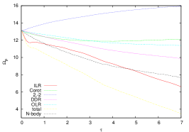
(a) $M_{b}=0.1$

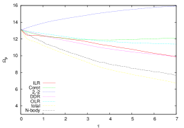
(b) $M_{b}=0.1$, 1/2 ILR

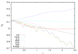
(c) $M_{b}=0.01$

Figure 17: The change in pattern speed $\Omega_{p}$ with scaled time $\tau$ as predicted by the one-dimensional evolution and N-body simulations. The contributions from five resonances ILR, $(2,-2)$, DRR, corotation and OLR are shown along with the total.

We compare a N-body self-consistent simulation of a bar that forms in a live disk(see Holley-Bockelmann et al., 2005, for details) to the one-dimensional perturbation theory calculations from §2.3.2. For these simulations, both the expansion centre and the quadrupole centre are at the origin. We eliminate the $l=1$ term from the expansion and apply only the quadrupole part of the bar perturbation. This eliminates issues of centring and combined halo-disk equilibria. We will treat these in paper II. The evolution of the pattern speed is computed by enforcing total conservation of angular momentum. The bar has a mass that is 10% of the dark matter enclosed within the bar radius and corotates at 3/2 of the bar radius. The bar is slowly turned on and off with the function $A(t)$ defined in §A. In Figure 17, we compare the evolution of the pattern speed in the N-body simulation to the prediction from the one-dimensional averaged perturbation theory. We also plot the contributions from the five most important resonances separately, calculated using the one-dimensional perturbation theory. Naively, the rate of secular evolution should be proportional to the perturbation amplitude. However, because of the slow and fast limits this simple scaling is broken. Nonetheless, we can remove some of the dependence on the turn on and turn off by plotting the pattern speed evolution in Figure 17 using the scaled time

$$\tau\equiv\int_{0}^{t}dt^{\prime}A(t^{\prime}).$$ (49)

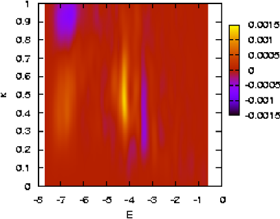
Figure 18: $\Delta L_{z}$ plot for the N-body simulation in Figure 17. Compare this with Fig. 7.

As one can also see from Figure 17a, the rate of pattern speed evolution predicted by the one-dimensional approach exceeds that in the N-body simulation owing to a stronger ILR contribution. As described in §2.3.4, the ILR is strongly nonlinear and the amplitude predicted by the one-dimensional solution is roughly a factor of two larger than for the three-dimensional solution. Figure 17b shows the same run but with the prediction for ILR decreased, in an ad-hoc way, by a factor of two, which gives a good correspondence between the theory and the simulation. Even with this decrease, we see that the torque is still dominated by the ILR and DRR. To check this interpretation, we decreased the bar amplitude by a factor of 10 to $M_{b}=0.01$. In this case, the ILR is not strongly nonlinear and we have a good correspondence between the prediction and the simulation without any ad hoc adjustment. Figure 18 shows the distribution of angular momentum change in phase-space as a result of the bar interaction. It looks very similar to the perturbation theory prediction in Figure 7 with the expected differences in the ILR.

4.4 A numerical testing ground

For testing ones own N-body code’s ability to properly evolve the bar-halo problem, we recommend reproducing some of the angular momentum exchange experiments performed here. For the bar–halo interaction, most researchers only check the evolution of the pattern speed with time. A more sensitive test, and one that is crucial to understanding the component–component interaction during the overall secular evolution, is to verify that each resonance is numerically converged. Comparing the distribution of the change in angular momentum in phase space is an effective tool to accomplish this goal (e.g. Figs. 7 and 5). These figures may be constructed as follows. For a spherical halo, the phase-space distribution function will be a function of energy and total angular momentum, $E$ and $J$. To make this plane rectangular, use the normalised angular momentum variable $\kappa\equiv J/J_{max}(E)$ so that $\kappa\in[0,1]$. For a spherical equilibrium, $J_{max}$ is the angular momentum of the circular orbit with energy $E$. This can be determined by finding the radius of the circular orbit $r_{c}$ by solving $E=v_{c}^{2}(r)/2+V(r)$ implicitly for $r$, where $v_{c}(r)\equiv\sqrt{r\,dV/dr}$ and then $J_{m}ax(E)=r_{c}v_{c}(r_{c})$. One then computes the change in angular momentum in some time interval on this plane. If resonant angular momentum transfer dominates the evolution, the change in angular momentum will follow the curves in $E$ and $\kappa$ defined by the commensurabilities. If scattering or more general non-resonant interaction dominates, the change in angular momentum will populate a broad area in this plane. This is only a rough guide; the ILR, for example, is broad $E$ and $\kappa$ owing to its special degeneracy (see Fig. 5). A $\Delta L_{z}$ plot can be made from an N-body simulation using the following procedure:

1. Save the state of the N-body phase space separated by a time interval that is small but of order of or larger than the orbital time scale. For the three-dimensional calculation (N-body simulation with fixed background potential), the evolution of the pattern speed may be compared with Figure 19 in §A.

2. For each orbit, compute the change in the $z$-component of the angular momentum, $\Delta L_{z}$. For figures in this paper, we compute $\Delta L_{z}$ for the entire simulation from before the bar is turned on until after it is turned off using $A(t)$ (eq. 51).

3. Use a density estimator to produce the distribution of $\Delta L_{z}$ over the phase space in the plane defined by $E$ and $\kappa$. Simple histograms will suffice but some tuning of bin sizes will be necessary to resolve the features.

Using this graphical tool, one may straightforwardly reproduce some of the examples presented here. Here are some recommended tests:

1. Compute the $\Delta L_{z}$ plots for the large bar used in §§3.2–3.3. The details of the bar perturbation are given in §A. The $\Delta L_{z}$ diagrams should be compared to Figures 7 and 5. One should attempt to identify each of the resonances.

2. The bar used for these examples is much larger than bars in Nature. This experiment should be repeated for a scale-length sized bar of moderate strength as described in §3.4. Ideally, check that their position and amplitude is converged by drastically increasing the particle number.

Since it is not possible to make particle number criteria that are appropriate for all problems, it is necessary to determine the criteria for each class of problem individually using the procedure that we outlined above. One should check these other scenarios against perturbation theory whenever possible. This is not always possible so an idealised experiment, i.e. one which imposes an approximate form of the perturbation and its time dependence, should suffice to verify the particle number criteria. Sometimes it is necessary to use a weaker form of the perturbation and in this case the derived particle number criteria can be scaled to the real problem. For these other perturbations, one can repeat the one- and three-dimensional computations outlined in §2 and compare them with N-body simulations. The perturbation theory allows one to separate the effects of the individual resonances and compute their locations and importance (e.g. Fig. 17). Numerical perturbation theory, i.e. the integration of the reduced one-dimensional equations of motion, bypasses most of the complications associated with solving the CBE while retaining all of the dynamics of the resonance interaction typical in canonical perturbation theory. Furthermore, this approach automatically includes any desired time dependence. All of the necessary details including a symplectic integration scheme are provided in §2.3.2. One may also compare individual orbits as in Figures 3 and 4 both to check of one’s perturbation theory calculation and to verify the choice of time step (see §3.3.4). Finally, a three-dimensional ensemble integration permits sampling a specific energy range in phase space with more particles than is possible with a full N-body simulation, as a test of convergence.

5 Summary

Secular evolution in galaxies is caused by intercomponent interactions possibly triggered by environmental disturbances. These interactions manifest themselves as large-scale asymmetric features such as spiral arms, bars, ovals, and lopsidedness. The dynamical mechanisms mediating the secular evolution in the collisionless components are resonantly driven.

The linear and nonlinear dynamics of a single particle in resonance and the features of orbit families in model potentials have been well understood using perturbation theory or numerical solutions of the equations of motion. However, an N-body simulation adds two additional complications. First, a simulation provides the ensemble result but the effect of a resonance on a particular orbit depends sensitively on initial conditions. The resulting angular momentum exchange in phase space at resonance has contributions of both signs depending on the orbits’ initial conditions. The ongoing secular evolution imposes a directionality that breaks the symmetry in the initial conditions. However, the simulation must have a sufficient number of particles in the vicinity of the resonance to obtain the correct net torque. Second, representation of the dark matter and stellar components by an unnaturally small number of particles leads to fluctuations in the gravitational potential. For modern simulations, the magnitude of these fluctuations yield a very long relaxation time but we have shown that the noise is sufficient to cause orbits to random walk through resonances. Of course, if some orbits walk out of the resonance, others walk in. However for some resonances, ILR in particular, orbits would like to linger near the resonance for many rotation periods. The noise prevents this and in doing so changes both the amplitude of the net torque and the location of the orbits in phase space receiving the torque. In this paper, we explored the details of the resonance mechanism and its manifestation in an N-body simulation from a rigorous kinetic theory point of view. We presented particle number criteria for each type of discreteness error and checked them with numerical experiments for the bar–halo interaction.

Both the coverage and noise criteria require a very large number of particles for important resonances. In the case of coverage, the net torque from such a resonance may not be discernible until the critical particle number is reached. In the case of noise, assuming that the coverage criterion is met, diffusion may force the resonant interaction into a different regime until the noise is reduced to the correct threshold by using a sufficient number of particles. In both cases, checking for convergence by (e.g.) doubling the number of particles may not be a good indicator. For example, Figure 11 shows that the ILR for a very large, albeit weak, bar is reduced by a factor of 3 and the angular momentum is transferred to orbits with higher energy (and therefore with large radii) for noise equivalent to $10^{6}$ particles. Scaling to a moderate strength disk-scale-length-sized bar would demand between $10^{8}$ and $10^{9}$ particles to attain the correct dynamical regime.

Although larger $N$ at fixed spatial resolution will reduce the fluctuations, many N-body practitioners choose to use their particle number to optimise the resolution since the cost of a simulation is driven by $N$. Unfortunately, this results in maximising the noise. For simulations of secular evolution, it is worth decreasing the spatial resolution and, thereby, use some of one’s particle resources to reduce noise. Alternatively, an expansion code allows us to directly control the spatial resolution and efficiently eliminate the high-spatial frequencies that dominate the noise. We have shown that this Poisson solver reduces the required number of particles to satisfy the noise criterion by several of orders of magnitude, in practise leaving only the coverage criteria. For this reason, we recommend this Poisson solver for treating problems of secular evolution and use it in Paper II to study the self-consistent evolution of the bar-perturbed halo. Of course, this method also has its price: one sacrifices adaptiveness and introduces some bias. However, in balance we have found it well suited to studying secular evolution.

The work presented here was the product of a sustained cycle of perturbation theory predictions followed by numerical experiments, and we needed many more cycles than anticipated! Our experience suggests that it may not be possible to provide a universal set of particle criteria for an arbitrary dynamical interaction for several reasons. The strength of the perturbation may change the morphology of the stable periodic orbits, the rate of secular evolution may change the resonance topology, and regimes such as fast and slow limit interactions in resonances may deceive N-body convergence tests. Rather, each secular mechanism must be studied in detail to develop a meaningful set of particle number criteria for that particular problem. Simulations alone are unlikely to be sufficient for a full understanding of the dynamics or even ascertaining convergence. The important astronomical processes of disk heating and secular bulge formation are worthwhile topics for this sort of future investigation.

Appendix A Details of the bar perturbation

Rather than apply a force from a full bar, we may capture the essence of the nonaxisymmetric interaction by considering the quadrupole component only. Laplace’s equation demands that the quadrupole part of the gravitational potential increases as $r^{2}$ for radii well within the bar and decreases as $r^{-3}$ far from the bar and, therefore, comes to a peak somewhere in between. We find that the following functional form

$$U_{22}=b_{1}{r^{2}\over 1+(r/b_{5})^{5}}$$ (50)

fits the quadrupole radial component for bars quite well. To be explicit, our halo is an NFW model with concentration $c=15$. We scale all radii and masses by the virial radius and virial mass, respectively. We fit equation (50) to a homogeneous ellipsoid with $b/a=1/5$ and $c/b=1/10$. The major axis for our main test case is chosen to be $a=r_{s}=1/15$. Our standard tests assume a bar mass of 1% of the dark-matter mass enclosed with the bar semi-major axis. This leads to the following values: $b_{1}=-70.4$, $b_{5}=0.0262$.

To compare with perturbation theory, we attempt to minimise transients by slowly turning on and off the perturbation using the following function:

$$A(t)={1\over 4}\left[1+\mathop{\rm erf}\nolimits\left({t-t_{0}\over\Delta t}\right)\right]\left[1+\mathop{\rm erf}\nolimits\left({t_{f}-t\over\Delta t}\right)\right]$$ (51)

where $t_{0}$ and $t_{f}$ are the turn and turn off times, respectively, and $\Delta$ is the width of the turn and turn off. The final perturbing potential is therefore:

$$H_{1}({\bf r},t)=A(t)\Re\left\{{U_{22}(r)Y_{lm}(\theta,\phi-\phi_{p}(t))}\right\}.$$ (52)

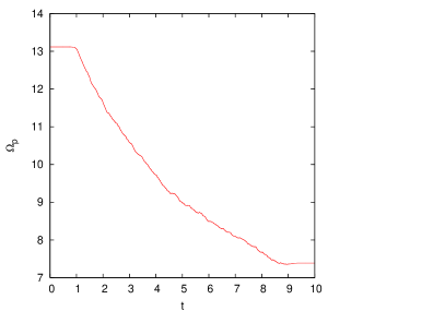
(a) $M_{b}=0.1,t_{0}=1,t_{f}=9,\Delta=0.2$

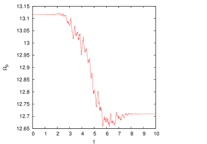
(b) $M_{b}=0.01,t_{0}=3,t_{f}=7,\Delta=1$

Figure 19:

The moment of inertia for the homogeneous ellipsoid about the minor axis is $I_{z}=M_{b}(a_{1}^{2}+a^{2})/5$ and the angular momentum of the bar is then $L_{bar}=I_{z}\Omega_{p}$. Let the $z$ component of angular momentum of the phase space be $L_{zp}$. Then in the three-dimensional direct integration of a phase-space ensemble, the pattern speed is derived by enforcing the conservation of momentum $L_{z\,tot}(t)=I_{z}\Omega_{p}(t)+L_{zp}(t)=L_{z\,tot}(0)=L_{bar}(0)+L_{zp}(0)$ to give: $\Omega_{p}(t)=(L_{bar}(0)+L_{zp}(0)-L_{zp}(t))/I_{z}$. Figure 19 shows the evolution of the pattern speed for the two bar examples from §3.2.

References

- Arnold (1978) Arnold V. I., 1978, Mathematical Methods of Classical Mechanics. Springer-Verlag, New York
- Athanassoula (2003) Athanassoula E., 2003, MNRAS, 341, 1179
- Binney & Tremaine (1987) Binney J., Tremaine S., 1987, Galactic Dynamics. Princeton University Press, Princeton, New Jersey
- Chirikov (1979) Chirikov B. V., 1979, Physics Reports, 52, 265
- Contopoulos & Grosbol (1989) Contopoulos G., Grosbol P., 1989, A&ARv, 1, 261
- Debattista (2002) Debattista V. P., 2002, in ASP Conf. Ser. 275: Disks of Galaxies: Kinematics, Dynamics and Peturbations Bar dynamical friction and disk galaxy dark matter content. pp 153–156
- Debattista & Sellwood (1998) Debattista V. P., Sellwood J. A., 1998, ApJL, 493, L5+
- Debattista & Sellwood (2000) Debattista V. P., Sellwood J. A., 2000, ApJ, 543, 704
- Eskridge et al. (2000) Eskridge P. B., Frogel J. A., Pogge R. W., Quillen A. C., Davies R. L., DePoy D. L., Houdashelt M. L., Kuchinski L. E., Ramírez S. V., Sellgren K., Terndrup D. M., Tiede G. P., 2000, AJ, 119, 536
- Fuchs (2001) Fuchs B., 2001, A&A, 368, 107
- Gao et al. (2004) Gao L., White S. D. M., Jenkins A., Stoehr F., Springel V., 2004, MNRAS, 355, 819
- Goldstein (1950) Goldstein H., 1950, Classical Mechanics. Addison-Wesley, Reading, Massachusetts
- Hernquist & Weinberg (1992) Hernquist L., Weinberg M. D., 1992, ApJ, 400, 80
- Holley-Bockelmann et al. (2005) Holley-Bockelmann K., Weinberg M. D., Katz N., 2005, MNRAS
- Jog (1992) Jog C. J., 1992, ApJ, 390, 378
- Jogee et al. (2004) Jogee S., Barazza F. D., Rix H., Shlosman I., Barden M., Wolf C., Davies J., Heyer I., et al., 2004, ApJL, 615, L105
- Lichtenberg & Lieberman (1983) Lichtenberg A. J., Lieberman M. A., 1983, Regular and Stochastic Motion. Springer
- Lynden-Bell & Kalnajs (1972) Lynden-Bell D., Kalnajs A. J., 1972, MNRAS, 157, 1
- Navarro et al. (1997) Navarro J. F., Frenk C. S., White S. D. M., 1997, ApJ, 490, 493
- Oguri & Lee (2004) Oguri M., Lee J., 2004, MNRAS, 355, 120
- Pawula (1967) Pawula R. F., 1967, Phys. Rev., 162, 186
- Press & Schechter (1974) Press W. H., Schechter P., 1974, ApJ, 187, 425
- Risken (1989) Risken H., 1989, The Fokker-Planck Equation. Springer-Verlag
- Sellwood (1981) Sellwood J. A., 1981, A&A, 99, 362
- Sellwood (2003) Sellwood J. A., 2003, ApJ, 587, 638
- Silverman (1986) Silverman B. W., 1986, Density Estimation for Statistics and Data Analysis. Chapman and Hall, London
- Spitzer (1987) Spitzer L., 1987, Dynamical Evolution of Globular Clusters. Princeton University Press, Princeton, New Jersey
- Toomre (1981) Toomre A., 1981, in Fall S. M., Lynden-Bell D., eds, , Normal Galaxies. Cambridge University Press, Cambridge, p. 111
- Touma & Tremaine (1997) Touma J., Tremaine S., 1997, MNRAS, 292, 905
- Tremaine & Weinberg (1984) Tremaine S., Weinberg M. D., 1984, ApJ, 282, L5
- Valenzuela & Klypin (2003) Valenzuela O., Klypin A., 2003, MNRAS, 345, 406
- Vesperini & Weinberg (2000) Vesperini E., Weinberg M. D., 2000, ApJ, 534, 598
- Weinberg (1985) Weinberg M. D., 1985, MNRAS, 213, 451
- Weinberg (1986) Weinberg M. D., 1986, ApJ, 300, 93
- Weinberg (1994) Weinberg M. D., 1994, AJ, 108, 1414
- Weinberg (1998a) Weinberg M. D., 1998a, MNRAS, 299, 499
- Weinberg (1998b) Weinberg M. D., 1998b, MNRAS, 297, 101
- Weinberg (2001) Weinberg M. D., 2001, MNRAS, 328, 311
- Weinberg (2004) Weinberg M. D., 2004, in ASP Conf. Ser. 317: Milky Way Surveys: The Structure and Evolution of our Galaxy Finding the Milky Way in 2MASS. p. 129
- Weinberg & Katz (2002) Weinberg M. D., Katz N., 2002, ApJ, 580, 627
- Weinberg & Katz (2005) Weinberg M. D., Katz N., 2005, MNRAS, to be submitted (Paper II)