Measurement of Noisy Absorption Lines using the Apparent Optical Depth Technique

Abstract

To measure the column densities of interstellar and intergalactic gas clouds using absorption line spectroscopy, the apparent optical depth technique (AOD) of Savage & Sembach (1991) can be used instead of a curve-of-growth analysis or profile fit. We show that the AOD technique, whilst an excellent tool when applied to data with good S/N, will likely overestimate the true column densities when applied to data with low S/N. This overestimation results from the non-linear relationship between the flux falling on a given detector pixel and the apparent optical depth in that pixel. We use Monte Carlo techniques to investigate the amplitude of this overestimation when working with data from the Far Ultraviolet Spectroscopic Explorer (FUSE) and the Space Telescope Imaging Spectrograph (STIS), for a range of values of S/N, line depth, line width, and rebinning. AOD measurements of optimally sampled, resolved lines are accurate to within 10% for FUSE/LiF and STIS/E140M data with S/N$\gtrsim$7 per resolution element.

1. Introduction

The apparent optical depth (AOD) method (Savage & Sembach, 1991; Sembach & Savage, 1992) has gained substantial popularity as a means of converting velocity-resolved flux profiles into column density measurements for interstellar and intergalactic absorption lines. The method offers a quick and convenient way of determining reliable interstellar column densities from unsaturated lines without having to follow a full curve-of-growth analysis or detailed component fit, and without demanding prior knowledge of the component structure. Accurate column densities are important for studies of elemental abundances and physical conditions in diffuse gas in space.

In the AOD method, a velocity-resolved flux profile $F(v)$ is converted to an apparent optical depth profile $\tau_{a}(v)$ using the relation:

$$\tau_{a}(v)={\mathrm{l}n}[F_{c}(v)/F(v)],$$ (1)

where and $F(v)$ and $F_{c}(v)$ are the observed line and continuum fluxes at velocity $v$, respectively. This apparent optical depth profile can then be converted to an apparent column density profile according to

$$N_{a}(v)=3.768\times 10^{14}(f\lambda)^{-1}\tau_{a}(v)\,\mathrm{cm^{-2}\,(km\,s^{-1})^{-1}},$$ (2)

where $f$ is the oscillator strength of the transition and $\lambda$ is the transition wavelength in Angstroms (Savage & Sembach, 1991). The total apparent column density between two velocity limits $v-$ and $v+$ is then simply $N_{a}=\int_{v-}^{v+}N_{a}(v)\mathrm{d}v$. When two lines of different strength of the same ionic species are available, the AOD method can also be used to assess and correct for the level of saturation in the data, by comparing the apparent column density derived from the stronger line with that derived from the weaker line (Savage & Sembach, 1991; Jenkins, 1996).

The AOD method was originally developed for application to measurements of reasonably high signal-to-noise spectra (S/N$\gtrsim$20 per resolution element). The technique offers excellent results in these cases. However, spectroscopists are now using the method even when analyzing relatively low S/N data (e.g. Wakker et al., 2003). This paper deals with accounting for a systematic error that is introduced when applying the AOD method to noisy data, which can lead to an overestimation of the true column density of the absorbing species. The error arises because the logarithmic relationship between $\tau_{a}(v)$ and $F(v)$ (Eq. 1) will distort a Poisson noise component in the flux when converting into column density space, giving undue weight to the pixels where the noise has resulted in high optical depths; this effect tends to exaggerate the estimate of $N_{a}$. We present simulations investigating the accuracy of $N_{a}$ determinations as a function of line depth and S/N, together with the separate effects of line width and rebinning.

2. Simulations

We ran Monte Carlo simulations of the measurement of noisy absorption lines to investigate the amount by which noise in the data leads to overestimation of $N_{a}$. Our models were run with two simulated experimental setups, representing the Far Ultraviolet Spectroscopic Explorer (FUSE) LiF (Sahnow et al., 2000) and Space Telescope Imaging Spectrograph (STIS) E140M (Woodgate et al., 1998) configurations. The FUSE/LiF setup is parameterized by a Gaussian instrumental line spread function with FWHM=20 km s^-1 ($\sigma_{ins}=8.5$ km s^-1) and velocity pixels 2.0 km s^-1 wide. The STIS/E140M configuration has FWHM=6.8 km s^-1 ($\sigma_{ins}=2.9$ km s^-1) and 3.2 km s^-1 pixels. Our models simulate the measurement of an absorption line whose intrinsic optical depth profile is a single-component Gaussian, centered for convenience at 0 km s^-1, and normalized to a peak optical depth of $\tau_{0}$, i.e. $\tau(v)=\tau_{0}e^{-v^{2}/2\sigma_{line}^{2}}$. We run models for two line width cases: resolved ($\sigma_{line}=2\sigma_{ins}$) and marginally resolved ($\sigma_{line}=\sigma_{ins}$) The AOD method is known to underestimate the column density for unresolved lines, when no allowance is made for the effects of unresolved saturation [see Table 5 of Savage & Sembach (1991)].

For a grid of different intrinsic central line depths $d_{line}$ we converted the optical depth profile to a normalized flux profile using $F_{norm}=e^{-\tau(v)}$, where the intrinsic central optical depth $\tau_{0}=-\mathrm{ln}(1-d_{line})$. The flux profiles were then convolved with the instrumental broadening function; the effect of this process is to decrease the intrinsic line depth to an apparent line depth ($d$), and increase the intrinsic line width to an apparent line width ($\sigma$). We then added different levels of random noise (drawn from a Gaussian distibution) to the data, scaled so that the S/N in the continuum reached the desired levels when rebinned to pixels equal in size to the resolution element. In the line, we scaled down the random noise contribution by $\sqrt{F}$, in accordance with Poisson statistics.

We then rebinned the data by different factors, converted the profiles to $N_{a}(v)$ space, and finally integrated the profiles over velocity to yield $N_{a}$, as a function of line depth, noise, and rebinning factor. The velocity integration limits used are $\pm 2.5\sigma$ around the line center, corresponding to the points where the line recovers to 96% of the continuum in the absence of noise. These limits were chosen so as to reproduce the velocity integration ranges used in practice, determined by comparing the line widths and velocity integration ranges from a large spectroscopic data set (the FUSE O VI survey; Wakker et al., 2003). For each model run, we determined the ratio of $N_{a}$ to $N_{true}$, where $N_{true}$ is the true column density of the simulated component, then repeated the process 500 times; the mean overestimation factor $<N_{a}>/N_{true}$, together with its dispersion, is then used in our results.

For very optically thick lines, the random error can take the flux below zero, corresponding to negative $N_{a}(v)$, which has no physical meaning. Therefore, a cutoff must be used, whereby all points with $F(v)$ less than some value are placed at that value (in our case, 1% of the continuum). The cutoff value selected will depend on the reliability of the scattered light and background corrections for the particular instrument providing the observations.

3. Results

Figure 1 shows a graphical example of the overestimation process for a resolved line with an intrinsic depth of 0.8, measured with FUSE. In the left column we show how the spectra would appear at different S/N levels, ranging from S/N=$\infty$ at the bottom to S/N=5 at the top. Note that we quote the S/N per resolution element, rather than the S/N at the level of rebinning shown. The two are related by (S/N)_res.elem.=$\sqrt{}$(number of bins per resolution element) $\times$(S/N)_bin. We verified this relation by measuring the S/N of the model spectra at different binning levels. In the next three columns we show the profiles in apparent column density space after different levels of rebinning.

In Figure 2 we display the results of different parameter cases using a color-coded plot: resolved lines with FUSE (top left), marginally resolved lines with FUSE (top right), resolved lines with STIS (bottom left), and marginally resolved lines with STIS (bottom right). Within each panel, we show the overestimation factor as a function of signal-to-noise ratio and apparent line depth (both easily measurable quantities), for three different rebinning cases. In each panel, we have not shaded in regions that correspond to non-significant detections, i.e. those with $W_{\lambda}<3\sigma(W_{\lambda})$; the minimum depth line that can be considered significant is proportional to (S/N)^-1, since at low S/N shallow lines will not be distinguished from the noise. Using Figure 2 an observer can find the likely error on $N_{a}$ in a line with a given depth, width, and S/N, and correct for it. The overestimation factors for a range of cases are also presented in Tables 1 and 2, for FUSE/LiF and STIS/E140M data, respectively. Upon request we can also provide an IDL code that returns the overestimation factor when given the measured S/N, apparent line depth, and apparent line width.

4. Discussion

The effects of several parameters combine to produce the trends seen in Tables 1 and 2 and Figures 1 and 2: S/N, level of rebinning, spectral resolution, line width, and line depth. We discuss each separately in this section.

• Low S/N and Rebinning – the non-linear distortion of the $N_{a}(v)$ profile and resulting overestimate of $N_{a}$ becomes worse as the S/N decreases (Fig. 1). Rebinning the spectrum before measurement can lessen the distortion, since the rebinning process increases the effective S/N. Once the data is rebinned to a level coarser than the resolution element, the gain in the $N_{a}$ accuracy is made at the expense of resolution, so that kinematic information is given up. However, if the absorption line before rebinning is fully or marginally resolved, and if one is more interested in obtaining an accurate column density than obtaining knowledge about the detailed shape of the line profile, then overbinning is justified at low S/N. AOD measurements made at optimum sampling (two rebinned pixels per resolution element) on FUSE and STIS data are overestimated by less than 10% for S/N per resolution element $\gtrsim$7. For data with lower S/N, rebinning beyond the resolution element will likely increase the accuracy of the derived column density.

• Lack of Resolution and Line Width – for marginally resolved lines, the apparent column density tends to underestimate the true column density at high line depths (purple shading on the right hand panels in Figure 2), since the high optical depth points are smoothed out to lower apparent optical depths by the instrumental blurring. This effect therefore works in the opposite sense to the S/N effect. The more unresolved the line is (i.e., the lower $\sigma_{line}/\sigma_{ins}$), the worse this effect becomes. Even full saturation can be hidden by the effects of instrumental broadening. Savage & Sembach (1991) and Jenkins (1996) discuss how this unresolved saturation can be corrected for when observations exist for more than one line of an ion. For resolved lines, increasing the ratio $\sigma_{line}/\sigma_{ins}$ above 2 increases the number of pixels susceptible to noise and hence increases $<\!N_{a}\!>/N_{true}$ slightly for a given S/N and line depth (by a few percent if $\sigma_{line}/\sigma_{ins}=4$); however, since the dependency on width is weak, we present results for two line width cases only.

• Line Depth – for a given S/N and line width, the overestimation factor is worse for shallow lines than for deep lines. This is because the noise is Poissonian, so a pixel with low optical depth (shallow) has a higher error on the flux than a pixel with high optical depth (deep). For very deep lines, the cutoff used to eliminate negative pixels underestimates the optical depth in very opaque parts of the profile. This effect works in the opposite sense to the S/N effect, so that measurements of very deep ($F(v)/F_{c}(v)\leq 0.10$) lines at low S/N are distorted by two competing effects. Note that if the noise were random rather than Poissonian (i.e. independent of the flux), the overestimation effect on deep lines would become worse since the flux errors deep in the lines are larger.

In Figure 3 we show the histogram of $N_{a}/N_{true}$ for one particular run (FUSE/LiF, $\sigma_{line}=2\sigma_{ins}$, S/N=8, intrinsic depth=0.5, 500 runs) for three levels of rebinning. The overestimation factor has a Gaussian distribution, with a mean that decreases with rebinning. For any given absorption profile, the overestimation can take a range of values. We therefore advise a conservative error estimate when correcting for the overestimation.

We note that the non-linear S/N distortion effect discussed here can influence the detailed intercomparisons of $N_{a}(v)$ profiles of the same ion. Therefore, corrections for line saturation based on comparing $N_{a}(v)$ profiles of weak and strong lines may not be valid for low S/N observations.

In their survey of O VI absorption in the Galactic halo and high-velocity clouds, Wakker et al. (2003) rebinned FUSE data with S/N$<$10 per resolution element by 5 pixels, and noisier data by up to 20 pixels, before measurement with the AOD technique. Our modelling shows that this was the correct procedure for measuring accurate O VI column densities, and we endorse a similar treatment of low S/N data in future studies. Without this rebinning, the column density measurements along sight lines with noisy spectra could be inflated by more than 20%.

Acknowledgements The authors wish to thank Ken Sembach and Chris Howk for useful discussions. This research has been supported by NASA through grant NNG04GC70G to BDS and grant NAG5-7444. BDS also acknowledges support from the University of Wisconsin Graduate School.

Table 1Simulation Results - FUSE/LiF

stringIntrinsicstring		stringApparentstring		S/N	string$<N_{a}/N_{true}>$string
FWHM	Depth	FWHM	Depth		3 pixel rebin	5 pixel rebin	10 pixel rebin
(km s-1)	(%)	(km s-1)	(%)		(6 km s-1 bins)	(10 km s-1 bins)	(20 km s-1 bins)
40.0	20	45.8	18	10	1.20$\pm$0.51	1.11$\pm$0.49	1.07$\pm$0.52
				8	1.32$\pm$0.69	1.16$\pm$0.64	1.09$\pm$0.68
				6	1.73$\pm$1.05	1.37$\pm$0.91	1.24$\pm$0.91
				4	3.18$\pm$2.14	2.02$\pm$1.70	1.49$\pm$1.47
40.0	50	47.8	45	10	1.07$\pm$0.20	1.04$\pm$0.19	1.01$\pm$0.20
				8	1.13$\pm$0.27	1.05$\pm$0.24	1.01$\pm$0.24
				6	1.29$\pm$0.44	1.13$\pm$0.38	1.04$\pm$0.35
				4	1.92$\pm$0.77	1.49$\pm$0.70	1.20$\pm$0.56
40.0	99	61.1	97	10	0.87$\pm$0.07	0.85$\pm$0.07	0.80$\pm$0.08
				8	0.90$\pm$0.09	0.87$\pm$0.09	0.81$\pm$0.10
				6	0.93$\pm$0.10	0.89$\pm$0.11	0.83$\pm$0.12
				4	1.00$\pm$0.16	0.94$\pm$0.16	0.85$\pm$0.17
20.0	20	28.6	14	10	1.21$\pm$0.81	1.11$\pm$0.81	1.04$\pm$0.87
				8	1.35$\pm$1.03	1.19$\pm$1.01	1.05$\pm$1.06
				6	1.78$\pm$1.57	1.41$\pm$1.44	1.18$\pm$1.44
				4	3.42$\pm$3.35	2.15$\pm$2.71	1.45$\pm$2.34
20.0	50	29.3	37	10	1.03$\pm$0.30	0.99$\pm$0.31	0.94$\pm$0.30
				8	1.11$\pm$0.42	1.04$\pm$0.41	0.97$\pm$0.40
				6	1.27$\pm$0.62	1.12$\pm$0.56	0.99$\pm$0.52
				4	2.06$\pm$1.34	1.56$\pm$1.18	1.18$\pm$0.92
20.0	99	34.2	89	10	0.67$\pm$0.09	0.63$\pm$0.08	0.56$\pm$0.07
				8	0.69$\pm$0.12	0.65$\pm$0.11	0.57$\pm$0.08
				6	0.75$\pm$0.16	0.69$\pm$0.15	0.58$\pm$0.12
				4	0.88$\pm$0.25	0.79$\pm$0.26	0.64$\pm$0.23

Note. — The FUSE/LiF spectrograph has FWHM_ins=20 km s^-1 and pixel size 2.0 km s^-1. The upper and lower halves of this table represent fullly resolved and marginally resolved lines, respectively.

Table 2Simulation Results - STIS/E140M

stringIntrinsicstring		stringApparentstring		S/N	string$<N_{a}/N_{true}>$string
FWHM	Depth	FWHM	Depth		1 pixel rebin	2 pixel rebin	3 pixel rebin
(km s-1)	(%)	(km s-1)	(%)		(3.2 km s-1 bins)	(6.4 km s-1 bins)	(9.6 km s-1 bins)
13.6	20	15.6	18	10	1.11$\pm$0.52	1.04$\pm$0.54	1.03$\pm$0.53
				8	1.16$\pm$0.70	1.04$\pm$0.70	1.02$\pm$0.71
				6	1.48$\pm$1.00	1.28$\pm$0.97	1.21$\pm$0.94
				4	2.11$\pm$1.81	1.46$\pm$1.52	1.29$\pm$1.43
13.6	50	16.2	45	10	1.03$\pm$0.18	1.00$\pm$0.19	0.98$\pm$0.19
				8	1.06$\pm$0.25	1.01$\pm$0.24	0.98$\pm$0.23
				6	1.11$\pm$0.36	1.02$\pm$0.34	0.99$\pm$0.33
				4	1.44$\pm$0.69	1.14$\pm$0.53	1.06$\pm$0.48
13.6	99	20.8	97	10	0.87$\pm$0.08	0.82$\pm$0.08	0.75$\pm$0.07
				8	0.89$\pm$0.09	0.84$\pm$0.09	0.76$\pm$0.09
				6	0.91$\pm$0.11	0.85$\pm$0.12	0.78$\pm$0.13
				4	0.96$\pm$0.16	0.87$\pm$0.17	0.81$\pm$0.18
6.8	20	9.7	14	10	1.10$\pm$0.78	1.02$\pm$0.81	1.01$\pm$0.85
				8	1.21$\pm$1.05	1.09$\pm$1.08	1.05$\pm$1.16
				6	1.43$\pm$1.45	1.24$\pm$1.48	1.17$\pm$1.56
				4	2.50$\pm$2.98	1.76$\pm$2.48	1.55$\pm$2.35
6.8	50	10.0	37	10	0.98$\pm$0.28	0.94$\pm$0.30	0.92$\pm$0.31
				8	1.04$\pm$0.37	0.99$\pm$0.37	0.95$\pm$0.38
				6	1.09$\pm$0.51	0.98$\pm$0.49	0.93$\pm$0.51
				4	1.52$\pm$1.10	1.18$\pm$0.87	1.09$\pm$0.86
6.8	99	11.6	90	10	0.66$\pm$0.09	0.60$\pm$0.07	0.53$\pm$0.07
				8	0.67$\pm$0.12	0.60$\pm$0.10	0.52$\pm$0.09
				6	0.72$\pm$0.16	0.62$\pm$0.14	0.54$\pm$0.12
				4	0.84$\pm$0.26	0.69$\pm$0.25	0.58$\pm$0.21

Note. — STIS/E140M has FWHM_ins=6.8 km s^-1 and pixel size 3.2 km s^-1. The upper and lower halves of this table represent fullly resolved and marginally resolved lines, respectively.

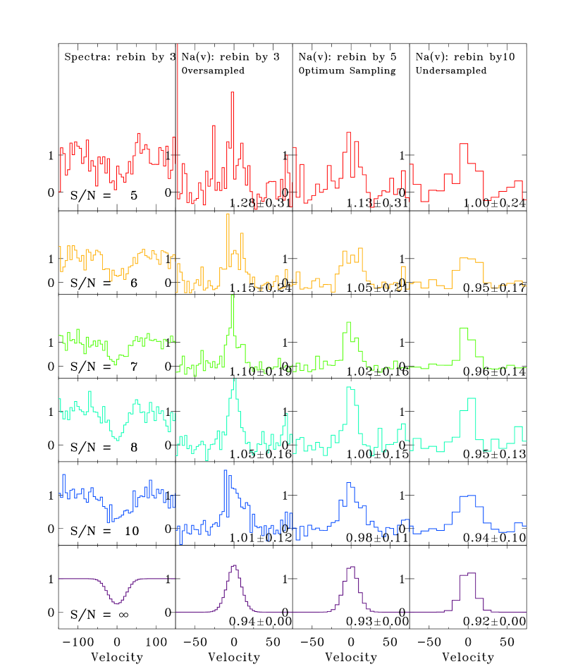
Figure 1.— Simulated spectra illustrating the effect by which $N_{a}$ is overestimated when the AOD technique is applied to noisy data, for resolved absorption lines observed with FUSE with an intrinsic central depth of 80%. The left column shows the simulated spectra with various levels of Poisson noise added. The next three columns show the effect of translating the noise into apparent column density space, after different levels of rebinning. The $N_{a}(v)$ profiles have been arbitrarily normalized for convenience. The numbers written in the corner of each panel represent the mean column density overestimation factor $<\!N_{a}\!>/N_{true}$ after 500 runs, together with its dispersion, where $N_{a}=\int N_{a}(v)\mathrm{d}v$ and $N_{true}$ is the true column density in the absorber. S/N is quoted per resolution element (corresponding in this case to the S/N at 10 pixel rebinning).

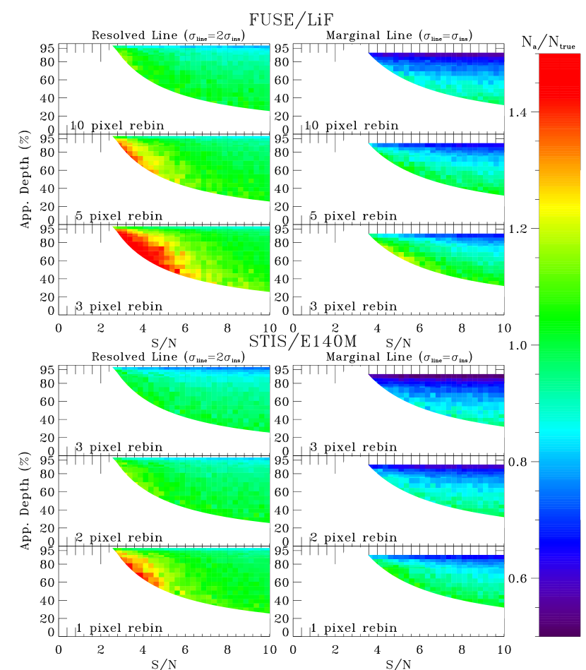
Figure 2.— Color-coded plots showing the column density overestimation factor $N_{a}/N_{true}$ as a function of signal-to-noise per resolution element, apparent line depth, and rebinning, for absorption lines measured using the AOD method in four cases: FUSE resolved lines (top-left), FUSE marginally resolved lines (top-right), STIS resolved lines (bottom-left), and STIS marginally resolved lines (bottom-right). Only lines with $>3\sigma$ equivalent width detections are included. Green regions show cases where the AOD method returns the column density correct to within 20%; blue and purple regions show where the AOD method will underestimate the true column density (unresolved lines, particularly at high depth); yellow and red regions show cases where AOD measurements lines will overestimate the column density at (low S/N, low depth).

Figure 3.— Histogram of $N_{a}/N_{true}$ for one model run, for three rebinning cases. There is a significant dispersion in overestimation factors for a given case. As the rebinning increases, the most likely value of $N_{a}/N_{true}$ approaches unity

References

- Jenkins (1996) Jenkins, E. B. 1996, ApJ, 471, 292
- Sahnow et al. (2000) Sahnow, D., et al. 2000, ApJ, 538, L7
- Savage & Sembach (1991) Savage, B. D., & Sembach, K. R. 1991, ApJ, 379, 245
- Sembach & Savage (1992) Sembach, K. R., & Savage, B. D. 1992, ApJS, 83, 147
- Wakker et al. (2003) Wakker, B. P., et al. 2003, ApJS, 146, 1
- Woodgate et al. (1998) Woodgate, B. E., et al. 1998, PASP, 110, 1183