HST/ACS WEAK-LENSING AND CHANDRA X-RAY STUDIES OF THE HIGH-REDSHIFT CLUSTER MS 1054-0321

Abstract

We present $Hubble$ $Space$ $Telescope$/Advanced Camera for Surveys (ACS) weak-lensing and $Chandra$ X-ray analyses of MS 1054-0321 at z=0.83, the most distant and X-ray luminous cluster in the $Einstein$ Extended Medium-Sensitivity Survey (EMSS). The high-resolution mass reconstruction through ACS weak-lensing reveals the complicated dark matter substructure in unprecedented detail, characterized by the three dominant mass clumps with the four or more minor satellite groups within the current ACS field. The direct comparison of the mass map with the $Chandra$ X-ray image shows that the eastern weak-lensing substructure is not present in the X-ray image and, more interestingly, the two X-ray peaks are displaced away from the hypothesized merging direction with respect to the corresponding central and western mass clumps, possibly because of ram pressure. In addition, as observed in our previous weak-lensing study of another high-redshift cluster CL 0152-1357 at $z=0.84$, the two dark matter clumps of MS 1054-0321 seem to be offset from the galaxy counterparts. We examine the significance of these offsets and discuss a possible scenario, wherein the dark matter clumps might be moving ahead of the cluster galaxies. The non-parametric weak-lensing mass modeling gives a projected mass of $M(r<1~{}\mbox{Mpc})=(1.02\pm 0.15)\times 10^{15}M_{\sun}$, where the uncertainty reflects both the statistical error and the cosmic shear effects. Our temperature measurement of $T=8.9_{-0.8}^{+1.0}$ keV utilizing the newest available low-energy quantum efficiency degradation prescription for the $Chandra$ instrument, together with the isothermal beta description of the cluster ($r_{c}=16\arcsec\pm 15\arcsec$ and $\beta=0.78\pm 0.08$), yields a projected mass of $M(r<1~{}\mbox{Mpc})=(1.2\pm 0.2)\times 10^{15}M_{\sun}$, consistent with the weak-lensing result.

1 INTRODUCTION

Galaxy clusters, the largest gravitationally bound systems in the universe, are believed to be the youngest physical structures, only recently dissociated from the Hubble expansion. They serve as powerful probes of cosmology and large scale structure formation because they retain a “memory” of their assembly history. Especially, many known high-redshift clusters at $z\sim 1$ show snapshots of their early stage of formation when the Universe was at approximately half its present age. Detailed studies of these distant, still-forming clusters can considerably enhance our understanding of the dynamical evolution of the cluster substructure.

Clusters of galaxies are composed of three major components: visible galaxies, a hot intracluster medium (ICM), and dark matter. The advent of high-resolution X-ray observatories have enabled remarkable progress in tracing the complicated thermodynamical structure of the ICM of a galaxy cluster, whereas weak-lensing particularly empowered by the $Hubble$ $Space$ $Telescope$ (HST) high-resolution observations is starting to yield a detailed distribution of dark matter. And extensive spectroscopic surveys of cluster fields by ground-based facilities with large aperture telescopes provide invaluable information on the distribution of the member galaxies as well as the kinematics of the cluster.

Weak-lensing analysis can provide the most direct measurement of the cluster mass distribution without any assumption about the dynamical phase of the cluster. However, under the simplified hypothesis that the cluster is in quasi-equilibrium, both the kinematics and the X-ray analyses can also independently be used to derive the mass properties of the target cluster.

A joint analysis of weak-lensing and X-ray measurements is a unique opportunity to investigate the interplay between the ICM and dark matter within the cluster. Because of their different natures, it is expected that these two components have somewhat dissimilar distributions within the cluster. The ICM, due to its collisional property, is subject to ram pressure, and shocks can be detected between merging sub-clusters where the transverse velocities exceed the sound speed. In addition, the frequent collisions between gas particles should evolve the system into a high degree of virialization on a relatively short time scale. On the other hand, cold dark matter, due to its hypothesized collisionless nature, is often believed to be traced by the cluster galaxies whose approximate dynamical behaviors are also collisionless.

However, it is very difficult to probe and test these theoretical speculations in detail for a distant cluster whose angular extent is only a few arcminutes. The substantial decrease in gravitational distortion of source galaxy images, because of the large distance between the observer and the lens, also requires a precise measurement of a galaxy shape with a careful removal of the instrumental artifacts.

Weak-lensing studies of high-redshift clusters benefit remarkably from the recent installation of the Advanced Camera for Surveys (ACS) on $HST$, which can resolve faint, more highly distorted distant galaxies (Jee et al. 2005, hereafter J05; Lombardi et al. 2005). Because of a high number density of background galaxies in the cluster field, the resulting mass reconstruction is capable of tracing the dark matter distribution in great detail.

In the current paper, we present the first weak-lensing study of MS 1054-0321 using the ACS observations and a reanalysis of the archival $Chandra$ X-ray data. MS 1054-0321, the most distant and X-ray luminous cluster in the $Einstein$ Extended Medium-Sensitivity Survey (Gioia et al. 1990; Henry et al. 1992; Gioia & Luppino 1994), has received profuse attention during the past decade because of its unusual richness at such a high-redshift (e.g., Gioia & Luppino 1994; Luppino & Kaiser 1997; Donahue et al. 1998; Tran et al. 1999; Clowe et al. 2000; van Dokkum 2000; Neumann & Arnaud 2000; Hoekstra et al. 2000; Jeltema et al. 2001; Joy et al. 2001; Vikhlinin et al. 2002; Gioia et al. 2004). The mere existence of such a massive cluster at $z\sim 0.83$ can impose strong constraints on the cosmological parameters, favoring a low-density Universe (e.g., Bahcall & Fan 1998; Donahue et al. 1998; Jeltema et al. 2001) or non-Gaussianity of the primordial density fluctuations (Willick 2000). The first $HST$ weak-lensing study of the cluster was performed by Hoekstra, Franx, & Kuijken (2000, hereafter HFK00) using WFPC2 observations. Their mass reconstruction revealed a complicated mass distribution characterized by three dominant clumps, in good spatial agreement with the cluster galaxy concentrations. However, the X-ray studies (e.g., Neumann & Arnaud 2000; Clowe et al. 2000; Jeltema et al. 2001) have demonstrated there are only two distinct X-ray peaks corresponding to the central and western clumps in the HFK00 mass distribution. The question whether the absence of the third peak is due to the low X-ray emission of the eastern clump or to an artifact in the weak-lensing mass reconstruction was raised (Jeltema et al. 2001). Because the Wide Field Channel (WFC) of ACS has twice the sampling resolution of the Wide Field (WF) chips of WFPC2 and a factor of 5 improvement in sensitivity, the use of ACS observations in the weak-lensing analysis can substantially improve the signal-to-noise ratio of the resulting mass reconstruction, therefore enabling us to test the significance of the cluster substructure presented by HFK00.

The X-ray study of MS1054 has an interesting history. Donahue et al. (1998) determined the temperature of the cluster to be very high ($T=12.3^{+3.1}_{-2.2}$keV) analyzing both $ASCA$ and $ROSAT$ data. Using $Chandra$ observations, Jeltema et al. (2001) obtained a slightly lower temperature $T=10.4^{+1.7}_{-1.5}$keV for the entire cluster. Joy et al. (2001) estimated the temperature of the cluster to be $T=10.4^{+5}_{-2}$keV from the Sunyaev-Zeldovich measurements. However, Vikhlinin et al. (2002) and Tozzi et al. (2003), using the same $Chandra$ data, obtained a somewhat lower temperature of $T=7.8\pm 0.6$keV and $T=8.0\pm 0.5$keV, respectively. A even lower temperature of $T=7.2^{+0.7}_{-0.6}$ keV is reported by Gioia et al. (2004) from the XMM-Newton observations. With the possibility of time variability excluded, these different temperature estimates simply demonstrate that the X-ray temperature measurement is sensitive to the analysis procedure as well as the maturity of the calibration of the instrument. For example, Gioia et al.(2004) were able to reproduce all the results of Jeltema et al. (2001) by duplicating the previous analysis procedures of the $Chandra$ data. However, when they altered the flare interval removal (resulting in shorter exposure time) and corrected for the quantum efficiency degradation, their results became consistent with the XMM-Newton measurements.

Despite these already copious X-ray studies in the literature, we present our reanalysis of the $Chandra$ archival data of MS 1054-0321 for the following two reasons. First, our understanding of the $Chandra$ instrument is still evolving and we find that the application of the new calibration data affects the derived physical quantities of the cluster. Second, we attempt to make a direct comparison between the results of the weak-lensing and the X-ray studies in terms of the total gravitating mass as well as the cluster substructure. Our previous ACS weak-lensing study (J05) of another high-redshift cluster CL 0152-1357 at a very similar redshift ($z\sim 0.84$) revealed a significant substructure interestingly offset from the X-ray and cluster galaxies, suggestive of an on-going merger of the two main clumps. Because MS 1054-0321 also possesses distinct substructure well traced by $Chandra$ and weak-lensing analyses, the current study is a good test to see whether we can detect similar offsets between the dark matter, ICM, and cluster galaxies.

Throughout the paper we assume a $\Lambda$CDM cosmology where $\Omega_{M}=0.27,\Omega_{\Lambda}=0.73,$ and $H_{0}=71$km $\mbox{s}^{-1}$. All the quoted uncertainties are at the 68% level.

2 OBSERVATION

2.1 ACS Data Reduction

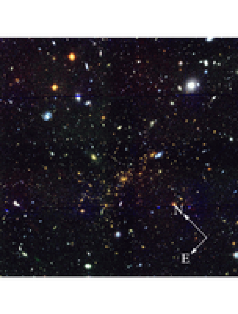
Figure 1: Color composite image of MS 1054-0321. The $v_{606}$, $i_{775}$, and $z_{850}$ intensities are represented by blue, green, and red colors, respectively. The red early-type galaxies of the cluster appear to form a filamentary structure, mainly stretched east-west.

The ACS/WFC images of MS 1054-0321 (Goto et al. 2005; Postman et al. 2005) consist of $2\times 2$ pointings observed in F606W, F775W, and F850LP (hereafter $v_{606}$, $i_{775}$, and $z_{850}$, respectively). The total exposure time per pointing is 2025 s for $v_{606}$, and 4440 s for $i_{775}$ and $z_{850}$. There is a $\sim 1\arcmin$ overlap between pointings. After the raw images were processed with the standard STScI CALACS pipeline, we used the “APSIS” ACS Guaranteed Time Observation (GTO) pipeline (Blakeslee et al. 2003) to perform cosmic ray rejection, geometric distortion correction, and image registration. The APSIS pipeline calculates image offsets by matching astronomical objects between pointings after applying a geometric distortion correction (Meurer et al. 2003). The Lanczos3 interpolation kernel, which creates less noise correlation and a sharper point-spread-function (PSF), is adopted. We present the color composite image of the cluster in Figure 1, which shows the $v_{606}$, $i_{775}$, and $z_{850}$ intensities with blue, green, and red colors, respectively. The main structure is notably delineated by the swath of the cluster red sequence. This orientation of the image indicated by the compass is maintained for all the subsequent figures throughout the paper.

Objects were detected using the SExtractor algorithm (Bertin & Arnouts 1996) by searching for at least five connected pixels above 1.5 times the local sky rms. SExtractor was executed on the detection image created by inverse variance weighting of all the three passband images. The final catalog is compiled after visually identifying and removing false objects such as saturated stars and CCD bleeding, diffraction spikes, clipped objects, HII regions in nearby galaxies, etc. Throughout the paper, we use SExtractor’s MAG_AUTO and MAG_ISO magnitudes for object’s magnitudes and colors, respectively. We determined the Galactic extinction (at $\alpha=10^{h}56^{m}53^{s}.59$, $\delta=-03\arcdeg 37\arcmin 45\arcsec.5$) to be E(B-V)=0.035 from the dust maps of Schlegel, Finkbeiner, & Davis (1998) and adjusted the $v_{606}$, $i_{775}$, and $z_{850}$ magnitudes by 0.103, 0.071, and 0.052, respectively. Figure 2 shows the magnitude distribution of all the objects in this final catalog.

2.2 Chandra Data Reduction

The X-ray observations of MS 1054-0321 were retrieved from the $Chandra$ X-ray Center (at http://cxc.harvard.edu/cda/). The cluster was observed on 2000 April 21-22 for $\sim 90,981$s with the back illuminated S3 chip of the Advanced CCD Imaging Spectrometer (ACIS-S3) at the focal plane temperature of -120$\arcdeg$C. We processed the raw X-ray events with the $Chandra$ Interactive Analysis of Observations (CIAO) software version 3.2 and the Calibration Database version 3.0 (CALDB), discarding bad events and $ASCA$ grades 1, 5, and 7. A new level-2 event file was created after the application of the charge transfer inefficiency (CTI) and the time-dependent gain corrections.

The background light curve was extracted from a circular annulus ($r=123\arcsec-151\arcsec$) centered at the assumed cluster center ($\alpha=10^{h}56^{m}58^{s}.6$ and $\delta=-03\arcdeg 37\arcmin 36\arcsec.7$) after masking out all the point sources detected by the CIAO wavelet detection program “wavdetect”. We used the $lc\_clean$ script (Markevitch 2003) to identify and remove the flare events, and the net exposure decreased to a total of $\sim 74,456$s. The same annulus was also taken for the background spectrum construction in spectral analyses.

3 WEAK-LENSING ANALYSIS

3.1 Luminosity of MS 1054-0321

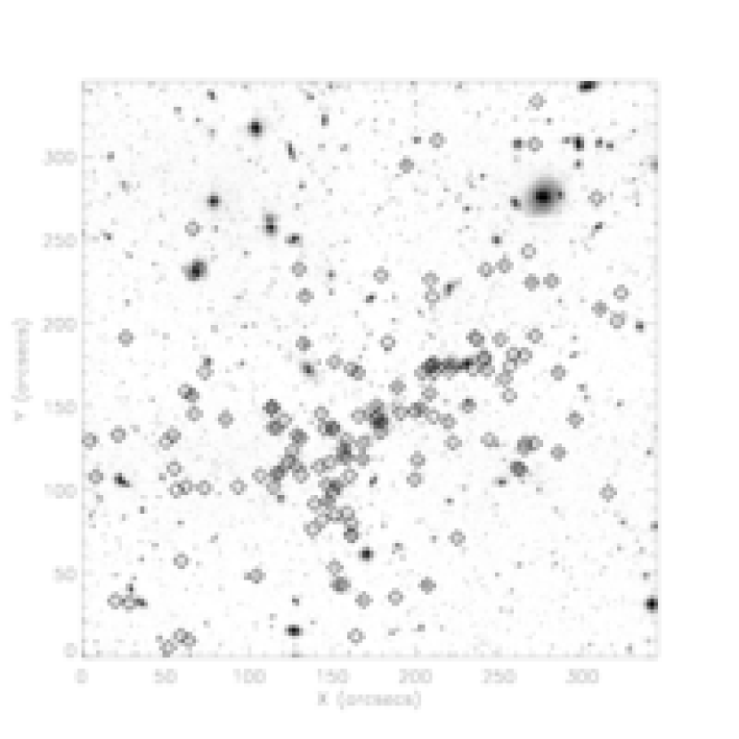
Figure 3: Spectroscopically confirmed cluster members. The galaxies whose spectroscopic redshifts are between $0.81<z<0.85$ are marked with squares.

We combine the extensive spectroscopic catalog of the MS 1054-0321 field (van Dokkum et al. 2000; Tran et al. in preparation) with the color-magnitude relation based on the ACS photometry to select the cluster members and estimate the rest frame B band luminosity of the cluster. We define a spectroscopically confirmed member as a galaxy whose redshift lies between $0.81<z<0.85$, which results in a total of 143 objects (Figure 3). We assume that the sample is almost complete for galaxies brighter than $z_{850}=22$ regardless of galaxy colors. For the intermediate magnitude range ($22<z_{850}<25$), we used the color-magnitude relation of the early type galaxies (Figure 4) while rejecting spectroscopically inconsistent members. Using the spectroscopic catalog of the field, we estimated that the blue cluster galaxies not included in this selection comprise nearly 50% of the cluster luminosity in this magnitude range. The contribution from the faint galaxies ($z_{850}>25$) was determined using the best-fit Schecter luminosity function. Adopting $M^{\star}=-21.47\pm 0.29$ and $\alpha=-0.87$ (Goto et al. 2004), we found that the light from this faint population accounts for $\sim 4$% of the final total luminosity.

The conversion of $i_{775}$ to the rest frame B is derived by performing a synthetic photometry using the Spectral Energy Distribution (SED) templates of Kinney et al. (1996). J05 established a similar transformation for Cl 0152-1357 at $z\simeq 0.837$, and here we extend the work of J05 by introducing the quadratic color term.

$$B_{rest} = i_{775}-(0.159\pm 0.163)(i_{775}-z_{850})^{2}-(0.224\pm 0.177)(i_{775}-z_{850})$$ (1)

$$+(0.728\pm 0.039)-DM,$$

where DM is the distance modulus of 43.605 at $z=0.83$ and the uncertainties are computed by assuming 2% photometric errors. Then the rest-frame B magnitude is converted to the luminosity by

$$\frac{L_{B}}{L_{B\sun}}=10^{0.4(M_{B\sun}-B_{rest})},$$ (2)

where $M_{B\sun}=5.48$ is the absolute B magnitude of the Sun.

Figure 5 shows the cumulative light profile of MS 1054-0321. Within 1 Mpc ($\sim 132\arcsec$) radius the total luminosity of the cluster is $8.2\times 10^{12}L_{B\sun}$. HFK00 estimated $1.0\times 10^{13}L_{B\sun}$ for $\Omega_{M}=0.3,\Omega_{\Lambda}=0,$ and $H_{0}=50\mbox{km~{}s}^{-1}$ cosmology. Iterating the above procedure with their cosmological parameters ($DM=44.09$) for comparison yields a total luminosity of $1.1\times 10^{13}L_{B\sun}$ within 1 Mpc ($\sim 105\arcsec$), which is slightly higher than the HFK00 estimation by $\sim$10%.

3.2 Correction for Instrumental Effects

Because weak-lensing is based on a statistical analysis of a population of very weakly distorted galaxy images, any instrumental artifact, usually of a comparable or even higher order of magnitude than the signal strength one is looking for, must be subtracted from first-hand measurements of object shapes. The geometric distortion of ACS, primarily due to the location of the instrument far from the telescope axis, is more significant than any of the previous $HST$ instruments. The uncorrected WFC image possesses an elongation of $\sim 8$% along the diagonal, thus causing the sky-projected pixel to appear rhombus-shaped. APSIS corrects the geometric distortion of WFC images using the latest detector distortion model (Meurer et al. 2003; Anderson 2002), which is derived from the observations of the core of 47 Tucanae. A fourth-order polynomial is used to characterize the distortion to an accuracy much better than 0.2 pixels over the entire field of view (Pavlovsky et al. 2004). Precise image alignment is also a principal requirement in a weak-lensing analysis because a slight registration error can imitate gravitational shears, inducing a coherent elongation of object shapes. APSIS calculates the image offsets by matching astronomical objects between different exposures. The typical shift uncertainty of $\sim 0.015$ pixels satisfies our analysis requirement.

The point-spread-function (PSF) of the WFC varies across the field even in the rectified image, and both the magnitude and orientation of the ellipticity change with the focus offset of the instrument (Krist 2003). In the previous work (J05), we demonstrated that the PSF model constructed from the 47 Tucanae observations can excellently describe the PSF pattern of the cluster field when a slight adjustment of the ellipticity is made. The PSF of ACS was decomposed via $shapelets$ (Bernstein & Jarvis 2002, hereafter BJ02; Refregier 2003) and the spatial variation was modeled by polynomial interpolation of the shapelet coefficients (see J05 for details).

Initial selection of stars in the MS 1054-0321 field was made using the half-light radius versus magnitude plot. After discarding defective stars by visual inspection, the list contained 94 good stars. We matched these stars in the cluster field to our model PSF derived from the 47 Tucanae field. The overall agreement is satisfactory, but there exist tiny, but systematic residuals, which are suspected to arise from the focus breathing of the instrument. We were able to further reduce these systematics by introducing the following ellipticity fine-tuning:

$$b_{pq}^{\prime}=\mbox{\bf{S}}_{\delta\eta}b_{pq},$$ (3)

where $b_{pq}(b_{pq}^{\prime})$ is the shapelet coefficient of the ACS PSF before (after) the adjustment and $\mbox{\bf{S}}_{\delta\eta}$ is the shear operator that modifies the ellipticity by $\delta\eta$ to improve the agreement. The evaluation of matrix elements of the shear operator S can be found in BJ02. The fine-tuning parameter $\delta\eta$ is held fixed within a field, but allowed to vary between exposures.

Figure 6 and 7 illustrate the PSF pattern observed in the $v_{606}$ mosaic image of the MS 1054-0321 field before and after the correction is applied. The correction is made by constructing a rounding kernel (Fischer & Tyson 1997; Kaiser 2000; BJ02) and convolving the stars with this kernel. However, as discussed in J05 (see also BJ02 and Seljak 2004), the rounding kernel method has several drawbacks compared to the momentum-based deconvolution. Therefore, we use this rounding kernel only for the verification of the PSF matching, and the actual correction is made through the deconvolution in shapelet space.

3.3 Shape Measurement

Galaxy shapes are decomposed via the following polar shapelets (see Refregier 2003 for Cartesian coordinates):

$$I(r,\theta)=\sum_{p,q\geq 0}b_{pq}\Psi_{pq}^{\sigma}(r,\theta)$$ (4)

$$\Psi_{pq}^{\sigma}(r,\theta)=\frac{(-1)^{q}}{\sqrt{\pi}\sigma^{2}}\sqrt{\frac{q!}{p!}}\left(\frac{r}{\sigma}\right)^{(p-q)}e^{i(p-q)\theta}e^{-r^{2}/2\sigma^{2}}L_{q}^{(p-q)}(\frac{r^{2}}{\sigma^{2}})\phantom{xxxxxx}(p\geq q)$$ (5)

$$\Psi_{qp}^{\sigma}=\bar{\Psi}_{qp}^{\sigma},$$ (6)

where $L_{q}^{m}(x)$ are the Laguerre polynomials.

Because our model PSF is also compactly described by these shapelets, we are able to perform the deconvolution through a simple matrix algebra:

$$\textbf{{b}}^{i}=\mbox{\bf{P}}^{-1}~{}\textbf{{b}}^{o},$$ (7)

where $\textbf{{b}}^{i}$, $\textbf{{b}}^{o}$, and P are the deconvolved image, the observed image, and the convolution matrix.

Then, we transform the PSF-corrected image $\bf{\mbox{b}}^{i}$ by applying translation, dilation, and shear operators:

$$\textbf{{b}}^{i\prime}=(\mbox{\bf{S}}_{\eta}\mbox{\bf{D}}_{\mu}\mbox{\bf{T}}_{z})\cdot\textbf{{b}}^{i},$$ (8)

where the S, D, and T are the shear, dilation, and translation operators defined in BJ02.

By requiring the above transformation to satisfy the condition $b^{i\prime}_{10}=b^{i\prime}_{11}=b^{i\prime}_{20}=0$, we can determine the ellipticity $\eta$ when both centroid and significance are optimized (BJ02).

3.4 Source Galaxy Selection

We select our source galaxies whose $v_{606}-z_{850}$ colors are bluer than $-0.123z_{850}+4.54$. In general, one desires to include as faint galaxies as possible because fainter galaxies are subject to greater distortion due to their higher cosmological distance from the lens. However, they also have larger uncertainties in their shape measurement arising from their poorer photon statistics in addition to greater correction factors for the removal of PSF effect. In order to establish a cutoff magnitude in our source galaxy catalog, we examined the variation of the lensing signal for three different magnitude samples: $bright$ ($24<z_{850}<26$), $faint$ ($24<z_{850}<28$), and $faintest$ ($24<z_{850}<30$). One useful way to compare the strength of the overall lensing signal is to inspect the tangential shear defined as:

$$\gamma_{T}=-\gamma_{1}\cos 2\phi-\gamma_{2}\sin 2\phi,$$ (9)

where $\phi$ is the position angle of the object with respect to the cluster center.

The amplitude of the tangential shear and the Einstein radius determined from the Singular Isothermal Sphere (SIS) fitting to each sample suggest that we can include background galaxies down to $z_{850}=28$ without diluting the signal (Figure 8). We excluded the shears $\gamma_{T}$ at $r<70\arcsec$ in the SIS fitting because we suspect that the measurement in this region is severely affected by the cluster substructure.

We investigated whether there also exists a strong color dependence in the signal amplitude. The galaxies in the $faint$ sample are divided into $blue$ $faint$ and $red$ $faint$ galaxies so that the sub-samples contain a roughly equal number of galaxies. As presented in Figure 9, we find the signal from $blue$ $galaxies$ are notably stronger, yielding an Einstein radius of $\theta_{E}=12.45\pm 1.25\arcsec$. HFK00 also found that their bluer galaxies create a larger amplitude in their WFPC2 weak-lensing analysis of MS 1054-0321. HFK00 suggested that their $bluer$ galaxies have a greater mean redshift. However, it is interesting to note that in the ACS weak-lensing of CL 0152-1357 we did not find such a shear excess in the $blue$ sample (J05). Considering the similar depth in both observations, it appears that the difference originates from the large scale structure of the field. In the following discussion we regard the $faint$ sample ($24<z_{850}<28$) (i.e., including both red and blue sources) as our best source catalog and the results hereafter are based on this catalog. The catalog contains a total of 5847 galaxies ($\sim 154~{}\mbox{arcmin}^{-2}$).

3.5 Redshift Distribution of Source Galaxies

The redshift distribution of source galaxies must be derived with extreme care because the critical density $\Sigma_{c}$ (mass unit) is a steep function of the source redshift for a high-redshift cluster. Consequently, it has been often considered a major source of uncertainty for weak-lensing mass estimation (e.g., Luppino & Kaiser 1997). However, the recent availability of a reliable photometric redshift catalog down to the faint limit of the source sample has remarkably stabilized the weak-lensing mass determination up to the cosmic variance.

In the current work, we utilize the photometric redshift catalog of the Ultra Deep Field (UDF), the deepest available patch of sky to date observed by both ACS and the Near Infrared Camera and Multi-Object Spectrometer (NICMOS). The detailed description of the generation of the photometric redshift catalog will be addressed in a forthcoming paper (D. Coe et al. in preparation); we give a brief description below.

We performed the PSF matching for different instruments and passbands using the stars present in the UDF field. The object catalog obtained from the ACS image is complemented with the objects only visible in the NICMOS images. For the galaxy SEDs, we selected the new templates of the Bayesian Photometric Redshift package (BPZ) (Benitez 2004), which are composed of the modified E, Sbc, Scd, and Im templates of Coleman, Wu, & Weedman (1980), two SB2 and SB3 starburst templates of Kinney et al. (1996), and one synthetic template from Bruzual & Charlot (2003). The last synthetic SED was added to account for very young, but faint starburst galaxies, for which a good observed template is not available.

In order to minimize the discrepancy caused by the field variation of the mean redshift of source galaxies, we selected the UDF galaxies by applying the same criteria as in the cluster field and determined the following $\beta$ for each magnitude bin:

$$\beta=\left<\mbox{max}(0,\frac{D_{ls}}{D_{s}})\right>,$$ (10)

where $D_{s}$ and $D_{ls}$ are the angular diameter distance from the observer to the source and from the lens to the source, respectively.

Because our cluster observation is shallower than the UDF, care must be taken not to ignore the incompleteness at faint limits, as well as the contamination by blue cluster galaxies. Noise was added to the UDF ACS images to mimic the S/N of the cluster observation, and the “mock” catalogs created from this degraded UDF ACS images were used to unbias the estimation of $\left<\beta\right>$ for $z_{850}>26$. For $z_{850}<26$ galaxies, we used the ACS photometry catalog from the Great Observatories Origins Deep Survey (GOODS; Giavalisco et al. 2004) as a control field to estimate the contamination from the blue cluster galaxies.

The final determination of $\left<\beta\right>=0.290$ corresponds to a single source plane at $\left<z\right>\simeq 1.325$. We also found that this single source plane approximation would cause an overestimation of the reduced shear by $(1+0.52\kappa)$ when the first order correction derived by Seitz & Schneider (1997) and HFK00 was employed. This correction becomes important at the dense region of the cluster where the assumption $\kappa<<1$ breaks down.

3.6 Weak-lensing Mass Estimation

First, we consider parameterized models for a description of the mass profile of MS 1054-0321. In order to minimize the effect of the cluster substructure, we use the tangential shears measured from $70\arcsec$ to $140\arcsec$ radii centered at the location of the BCG.

The SIS fit gives an Einstein radius of $\theta_{E}=11\arcsec.1\pm 1.\arcsec 0$ ($\sim 84$ kpc), yielding an aperture mass of $(9.6\pm 0.8)\times 10^{14}M_{\sun}$ within 1 Mpc radius. Under the same SIS assumption, this mass is translated to a velocity dispersion of $1150_{-51}^{+49}$ km$s^{-1}$. A similar Einstein radius of $11\arcsec.1\pm 2\arcsec.4$ is obtained when the Singular Isothermal Ellipsoid (SIE) model is fit instead. In addition, the position angle of $4\pm 11\arcdeg$ with respect to the x-axis of the image and the axis ratio of $b/a=0.51\pm 0.08$ are consistent with the elongation of the cluster substructure. Fitting an NFW profile to the tangential shears taken from $70\arcsec$ to $150\arcsec$ radii yields a concentration parameter of $c=3.2\pm 2.2$ and a core radius of $r_{s}=63\pm 28\arcsec$. Because these two parameters are not independent (i.e., they can be traded off with each other and the $\chi^{2}$ contours are highly elongated in the diagonal direction), a wide range of the parameter values can describe the observed shear profile without significantly altering the quality of the fit. Marginalizing with c=3.2, we obtain a projected mass of $M(r<1\mbox{Mpc})=(8.9\pm 0.4)\times 10^{14}M_{\sun}$.

For parameter-free estimation of the cluster mass profile, we use a conventional aperture mass densitometry as well as a rescaled ($\kappa\rightarrow\lambda\kappa+(1-\lambda)$) mass reconstruction (J05). We constrain a mean surface mass density of an annulus from $130\arcsec$ to $145\arcsec$ to be $\kappa=0.041+0.005$ utilizing the best-fit SIS parameters. Within 1 Mpc aperture radius, we obtain $(1.02\pm 0.04)\times 10^{15}M_{\sun}$ and $(1.01\pm 0.04)\times 10^{15}M_{\sun}$ from aperture mass densitometry and mass reconstruction, respectively.

We compare these various mass profiles in Figure 10. Note that the mass profile derived from the mass reconstruction agrees nicely with that from aperture mass densitometry. This remarkable agreement was also observed in the weak-lensing analysis of CL 0152-1357 in J05, and the use of the rescaled mass map ($\kappa\rightarrow\lambda\kappa+(1-\lambda)$ ) is now encouraged in the mass estimation of the substructure. The best-fit SIS profile describes the radial distribution of the cluster mass similar to the results from the parameter-free mass estimation whereas the NFW profile yields somewhat lower mass at large radii ($\sim 12$% at 1 Mpc).

HFK00 quoted an aperture ($r=1$ Mpc) mass of $(1.07\pm 0.12)\times 10^{15}M_{\sun}$ from the measurement of $\zeta(r)$ statistics in the $(\Omega_{M},\Omega_{\Lambda},h)=(0.3,0.7,0.5)$ universe. We find that their result is in good agreement with our aperture mass estimate of $(9.91\pm 0.42)\times 10^{14}M_{\sun}$ (when our result is reproduced under their cosmological parameters).

A caution must be made regarding the interpretation of the uncertainties quoted above. Although our weak-lensing analysis benefits considerably from the unprecedentedly high number of background galaxies, the quoted uncertainties here only reflects the statistical errors. In § 5.2 we discuss the importance of the foreground/background cosmic shear effects and estimate how much they can limit the accuracy of our cluster mass determination.

3.7 Mass-to-light Ratio Profile

We can combine the light and the mass profile to examine the radial behavior of the cluster mass-to-light ratio (Figure 11). The cumulative $M/L_{B}$ (open circle with error bar) increases rapidly at small radii ($r<50\arcsec$) and continues to rise rather slowly reaching $124\pm 5M_{\sun}/L_{\sun}$ (the uncertainty only reflects the statistical error in mass). at $r=1$Mpc. This pattern is quite different from that for CL 0152-1357, for which the cumulative $M/L_{B}$ arrives at its maximum at $r\sim 35\arcsec$ and decreases rather monotonically afterwards. The $M/L_{B}$ profile of CL 0152-1357 is very similar to that of an ensemble cluster compiled from the extensive kinematic studies of a large cluster sample (Carlberg et al. 1997; Katgert et al 2004). The outwardly increasing $M/L_{B}$ profile of MS 1054-0321 is also seen in HFK00 paper. The smoothed differential $M/L_{B}$ profile (i.e., $\delta M(r)/\delta L(r)$) shows the radial variation more markedly and the two $M/L_{B}$ “bumps” at $r\simeq 50\arcsec$ and $110\arcsec$ can be associated with the mass concentrations seen in the weak-lensing mass reconstruction.

Considering the luminosity evolution $\mbox{ln}(M/L_{B})\propto(-1.06\pm 0.09)z$ (van Dokkum & Stanford 2003; Holden et al. 2005), we can predict the $M/L_{B}$ value of the cluster at z=0. If the B-band luminosity decreases by $\sim 41$% from z=0.83 to z=0 (van Dokkum & Stanford 2003), the corresponding $M/L_{B}$ of MS 1054-0321 becomes $\sim 303M_{\sun}/L_{\sun}$ ($r<1$Mpc) in the present Universe. HFK00 obtained a slightly larger $M/L_{B}$ value of $320\pm 35~{}h_{71}M_{\sun}/L_{B\sun}$, but the result is still consistent with our $M/L_{B}$ estimation. They demonstrate that the average $M/L_{r}$ value of the 14 near-by clusters originally presented by Carlberg, Yee, & Ellingson (1997) becomes similar to the $M/L_{B}$ of MS 1054-0321 if $B-r\sim 1.1$ is taken into account.

3.8 Substructure

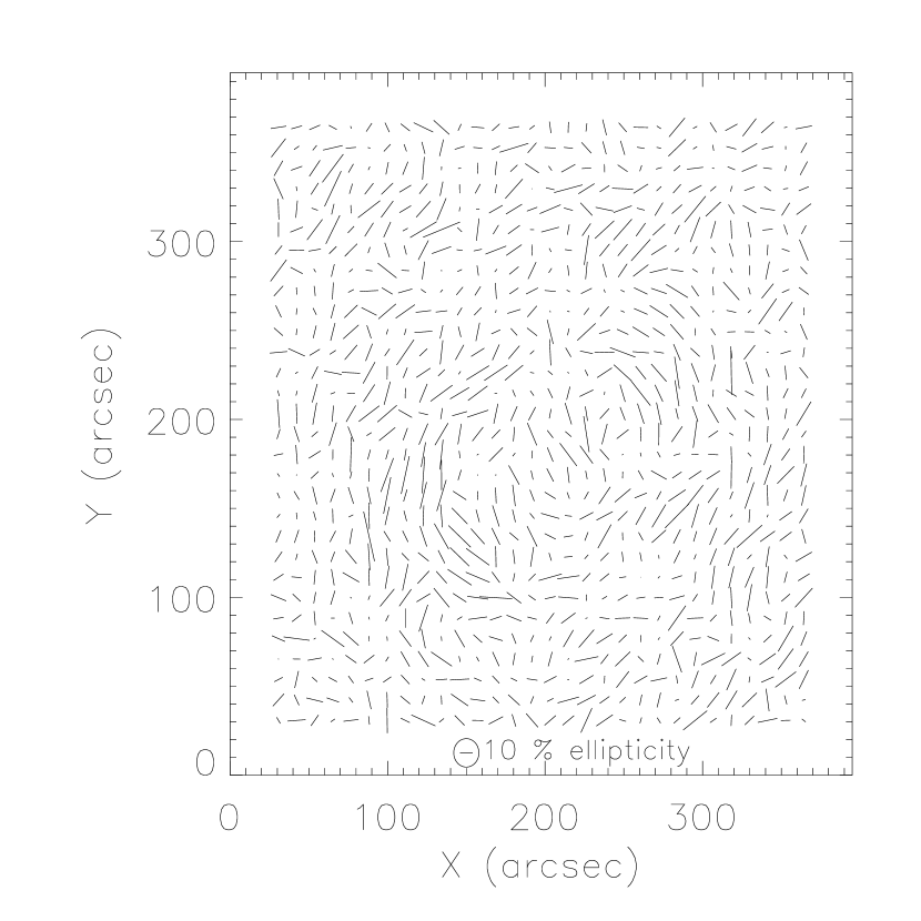
Figure 12: Ellipticity distribution of source galaxies. Each stick represents the weighted mean ellipticity of the background galaxies. Note the tangential alignments of “whiskers” around the cluster main body.

The whisker plot (Figure 12) demonstrates the weighted mean ellipticity distribution across the cluster field. The length of each whisker is proportional to the magnitude of the mean ellipticity of the source galaxies in the region and the position angle is expected to be aligned with the mean local shear. The presence of the lensing signal is obvious from the systematic patterns around the cluster galaxies.

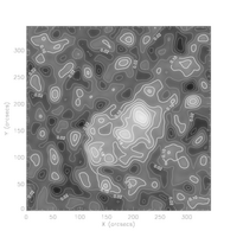
Figure 13: Rescaled mass reconstruction. Sheet-mass degeneracies are lifted using the SIS fit result. The mass map has been smoothed with a Gaussian kernel (FWHM $\sim 15\arcsec$). Because we do not vary the kernel size adaptively, the significance of the substructure is relatively low outside the main cluster body.

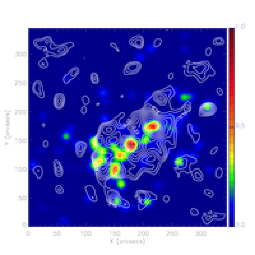
Figure 15: Mass contours overlaid on light distribution. The background is color-coded with the rest-frame B band luminosity of the spectroscopically confirmed cluster galaxies. We only display mass contours whose significance is approximately above 3 $\sigma$ ($\kappa>0.1$)

We present the weak-lensing mass reconstruction of MS 1054-0321 and its rms in Figure 13 and 14, respectively. The mass map is generated via the nonlinear reconstruction (Bartelmann 1995) with a significant modification to properly account for the rescaling ($\kappa\rightarrow\lambda\kappa+(1-\lambda)$) using the SIS fit result (J05). We smoothed the result with a $\mbox{FWHM}=10\arcsec$ Gaussian kernel The rms mass map is produced from 5000 mass reconstruction maps via Bootstrap resampling. The main body of MS 1054-0321 characterized by the three dominant mass peaks is manifest in the mass reconstruction. These three mass peaks were first identified by HFK00 in their weak-lensing analysis using WFPC2 observations (see §5.3 for comparison). A similar substructure can be obtained when the light distribution of the cluster galaxies is smoothed with a FWHM$\simeq 14\arcsec$ Gaussian kernel (we used a FWHM$\sim 10\arcsec$ kernel for the mass map). An overlay of the mass contour ($\kappa>0.1$) on top of this light distribution created from the confirmed cluster galaxies is presented in Figure 15. It is apparent that the cluster galaxies trace the cluster mass fairly well. The mass distribution over the eastern clump, unlike the other two mass clumps, seems to be somewhat complicated as is also indicated by the color-coded light distribution.

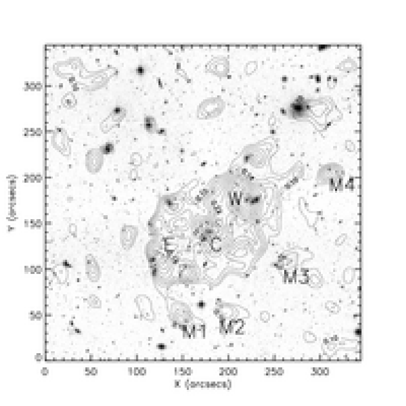
Figure 16: Mass contours overlaid on negative ACS image. Same as Figure 15 but with the background replaced with the negative ACS detection image. We identify 7 mass clumps (labeled W, C, E, M1, M2, M3 and M4) whose significance is high ($>3\sigma$) and the galaxy counterpart is unambiguous. Some of the unlabeled mass clumps seem to be associated with foreground galaxies.

We conservatively select four mass clumps outside the main body where the significance is above the $\sim 3\sigma$ level and the galaxy counterparts are not ambiguous (Figure 16). These four minor clumps (M1-4) are located south of the main clumps (C, W, and E) and they appear to be infalling groups onto the main cluster. Each of these minor clumps contain some bright early-type galaxies and its luminosity peak is close to the corresponding mass clump with an average offset of $\sim 6\arcsec$. Because of the relatively weak shear signal and thus low significance of the mass centroid of each mass peak, it is hard to infer the dynamics of the clump based on its mass-to-galaxy offset. It is interesting to note that in our previous investigation we also identified four minor mass clumps spatially correlated with the cluster member galaxies outside the main body of CL 0152-1357 at z=0.84 (J05). If these clusters are found to represent the typical clusters at this redshift, the presence of these hypothesized infalling groups can provide direct support of hierarchical structure formation.

Some of the rest of the minor mass peaks in our MS 1054-0321 mass reconstruction seem to be associated with foreground objects in the field, but here we confine our analysis only to mass clumps obviously related to the substructure of MS 1054-0321 at $z=0.83$.

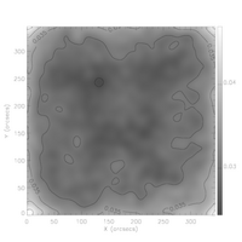
Figure 14: RMS map of mass reconstruction presented in Figure 13. The RMS is computed from 5000 bootstrap runs of mass reconstruction. Note that the RMS increases where the source galaxies are sparse, especially at the four corners.

Table 1 summarizes the properties of these mass clumps. The mass within $30\arcsec$ ($\sim 223$ kpc) aperture radius is measured from the rescaled mass map, and the mass uncertainty is calculated using the rms map (Figure 14) under the assumption that the mass pixels within the aperture are entirely correlated. The mass-to-light ratio is computed only counting the spectroscopically confirmed members. Therefore, the $M/L_{B}$ values quoted here correspond to the upper limits and in particular, for the minor clumps we suspect these $M/L_{B}$ values are largely overestimated because the incompleteness of the spectroscopic sample is higher for bluer cluster galaxies (Goto et al. 2005).

4 $CHANDRA$ X-RAY ANALYSIS

4.1 X-ray Substructure

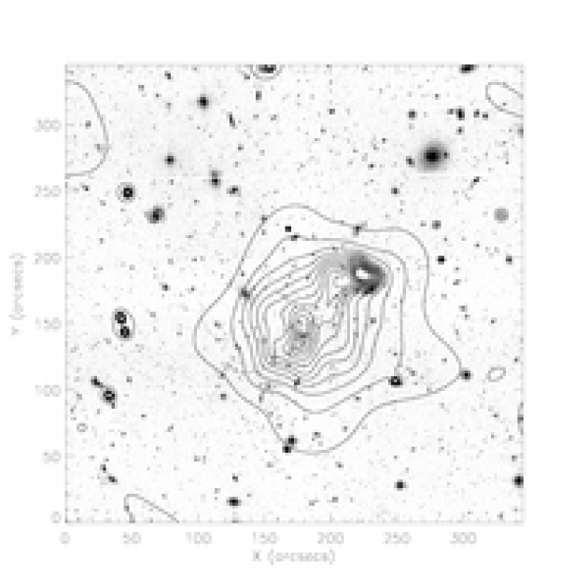
Figure 17: Chandra X-ray contours on top of ACS image. The exposure corrected X-ray image (0.8-7 keV photons) is adaptively smoothed with a minimum significance of 3 $\sigma$. The X-ray peaks are correlated with, but slightly offset from the cluster galaxies. The excellent agreements in point sources verifies the accurate image alignments between the two images.

We created an exposure corrected X-ray image by extracting 0.8-7 keV photons without excluding point sources. The image was then adaptively smoothed with the CIAO “csmooth” with a minimum significance of 3 $\sigma$. We carefully aligned the Chandra image with the ACS and the excellent coincidence of the X-ray point sources with the corresponding galaxies verifies the precise alignment between these two images (Figure 17). The resulting X-ray contours clearly show the substructure of the cluster reminiscent of the distribution of the member galaxies and dark matter. However, as noted by Jeltema et al. (2001), the $Chandra$ X-ray reveals only two clumps, which seem to be associated with the central and the western weak-lensing mass peaks. The absence of the eastern weak-lensing substructure in X-ray emission is also confirmed by the XMM-$Newton$ observations (Gioia et al. 2004). Interestingly, the locations of the two X-ray peaks are not in precise agreement with those of the BCGs as first indicated by Jeltema et al. (2001). Further discussion on this centroid offsets in addition to the absence of the eastern peak in the X-ray emission is deferred to § 5.6.

Although the X-ray peak close to the central dark matter clump was referred to as the “eastern” X-ray peak in Jeltema et al. (2001), hereafter we refer to the clump as the “central” peak to maintain a consistency with the previous weak-lensing substructure labeling. The central X-ray peak seems to be somewhat less concentrated than the western X-ray peak, possibly further resolved into two minor peaks. The X-ray contours obtained from the XMM-$Newton$ observations (Gioia et al. 2004) also indicate this possibility.

4.2 Cluster X-ray Temperature and Luminosity

The understanding of the X-ray temperature of MS 1054-0321 based on the $Chandra$ observatory evolves as new calibration data on the instrument becomes available. It has been realized that the degradation of the low energy quantum efficiency (QE) of the instrument is significant and possibly due to the molecular contamination of the ACIS optical blocking filters. This decline of the low energy sensitivity biases the temperature measurement upward unless accounted for. Based on the observed decay rate determined from the external calibration source, Chartas & Getman (2002) introduced a time dependent ACIS absorption model (ACISABS), which describes the degradation of the QE as a function of the number of days since the launch. Gioia et al. (2004) argued that the temperature measurement of MS 1054-0321 by Jeltema et al. (2001) suffered from the absence of this low-energy correction, being biased toward high temperature. However, the use of the ACISABS model was deprecated by CIAO as of CALDB 2.26 (released on 2 February 2004), and it is recommended that instead an area response file (ARF) be created with the calibration database that now properly reflects the time- and area-dependent QE degradation model. We observe that following this new procedure tends to yield a higher temperature than the ACISABS prescription.

Another important preprocessing for the spectral analysis includes careful background flare removal. The omission of the procedure also results in an overestimation of the cluster temperature. Although Jeltema et al. (2001) attempted to remove high background time intervals, their somewhat long net exposure time of $\sim 88$ ks compared to our result of $\sim 74$ ks indicates that flare identification was insufficient. Tozzi et al. (2003) and Gioia et al. (2004) also obtained relatively short net exposures of $\sim 80$ks and $\sim 67$ks, respectively.

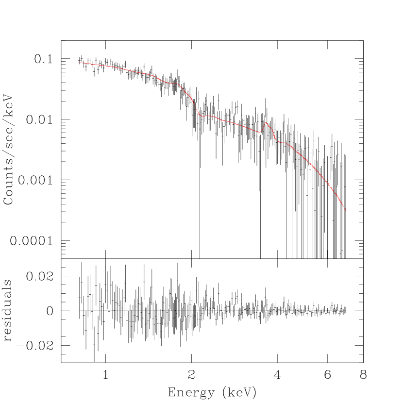
Figure 18: X-ray spectrum of MS 1054-0321 as a whole. The spectrum is taken from $90\arcsec$ aperture radius with the local background subtraction. Each spectral bin contains at least 20 counts. The best-fit MEKAL plasma model (solid) yields a cluster temperature of $T=8.9_{-0.9}^{+1.0}$ keV with a metal abundance of $Z/Z_{\sun}=0.30_{-0.12}^{+0.12}$.

We created the ARF and the redistribution matrix file (RMF) to account for the instrument response variation. The ARF file was generated using the new CIAO 3.2 tool $mkacisrmf$, which provides more accurate calibration at low energies ($<1keV$) than the previous CIAO script $mkarf$. However, because our spectral analysis was limited to the 0.8-7 keV range, we only observed marginal change ($\sim 0.2$ keV) due to this new prescription. We adopt the cluster center ($\alpha=10^{h}56^{m}58^{s}.6$ and $\delta=-03\arcdeg 37\arcmin 36\arcsec.7$) defined by Neumann & Arnaud (2000). The spectrum extracted from a circular region with a radius of $90\arcsec$ was fitted to the MEKAL plasma model (Kaastra & Mewe 1993; Liedahl, Osterheld, & Goldstein 1995). We froze the Galactic hydrogen column density and the redshift of the cluster at $N_{H}=3.6\times 10^{22}\mbox{cm}^{-2}$ (Dickey & Lockman 1990) and $z=0.83$, respectively. Figure 18 shows the best-fit thermal plasma spectrum, which yields a temperature of $T=8.9_{-0.8}^{+1.0}$ keV and a metal abundance of $Z/Z_{\sun}=0.30\pm 0.12$ with a reduced $\chi^{2}=0.63$ (206 degrees of freedom). Using the similar parameter constraints, Jeltema et al. (2001) found a temperature of $T=10.4^{+1.7}_{-1.5}$ keV whereas Gioia et al. (2004) reported that a temperature of $T=7.4^{+1.4}_{-0.9}$ keV was obtained when the two aforementioned corrections were applied to the $Chandra$ data. We verified that, if the ACISABS model was adopted instead, our temperature measurement decreased to $\sim 7.8$ keV, a result closer to the measurement of Gioia et al. (2004). In Table 2 we summarize the previous temperature measurements of MS 1054-0321 found in the literature.

From the best-fit spectra, we obtain the observed-frame flux of $F_{0.8-7.0~{}keV}=(5.9\pm 0.2)\times 10^{-13}\mbox{erg}~{}\mbox{cm}^{-2}~{}\mbox{s}^{-1}$ within a $90\arcsec$ radius. This becomes a rest-frame bolometric (0.01-40 keV) luminosity of $L_{X}=(3.1\pm 0.1)\times 10^{45}\mbox{erg}~{}\mbox{s}^{-1}$ after the k-correction to the rest-frame and the aperture correction to total are applied.

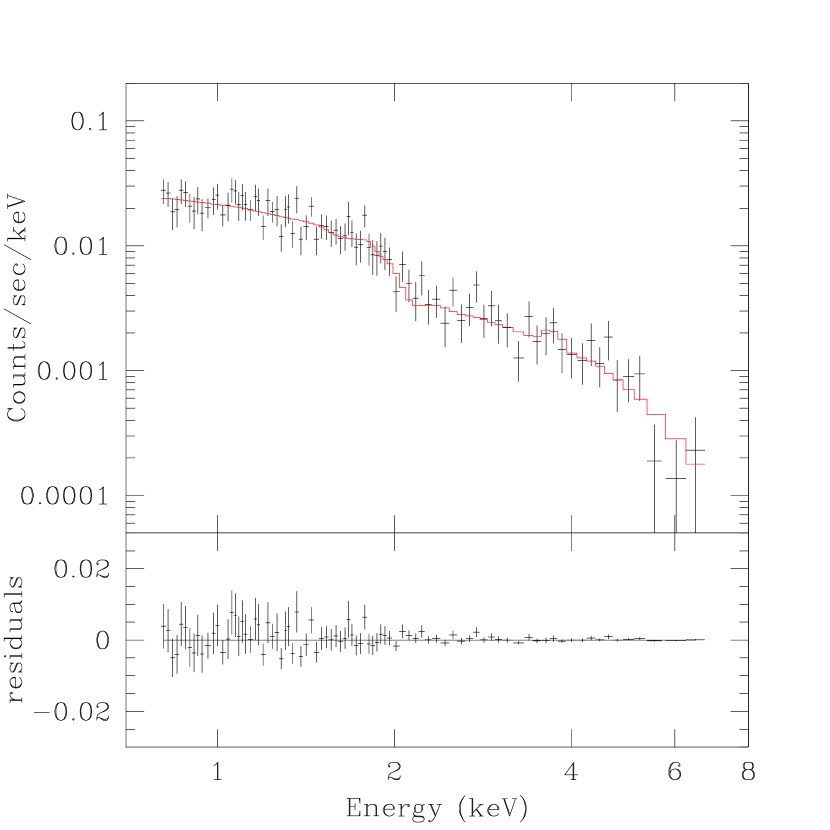
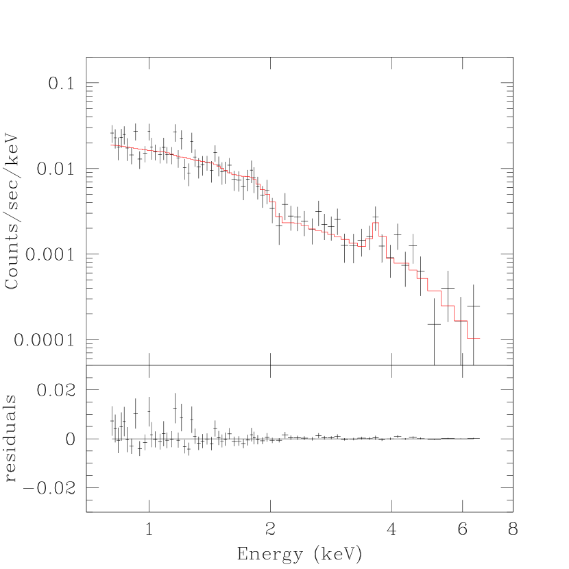
Figure 19: X-ray spectra of the individual X-ray clumps. The central clump (left panel) has a higher temperature ($10.7_{-1.7}^{+2.1}$ keV) than the western X-ray clump (right panel; $7.5_{-1.2}^{+1.4}$ keV). The best-fit MEKAL plasma model is represented by solid line. The iron emission line is more pronounced in the spectrum of the western clump ($Z=0.47_{-0.23}^{+0.24}Z_{\sun}$) while the feature is weaker for the central clump ($Z=0.16_{-0.16}^{+0.19}Z_{\sun}$).

We find that the temperature of the central peak is higher than that of the western peak (Figure 19;Table 3) as was also noticed by Jeltema et al. (2001). Our temperature measurements of $T=10.7_{-1.7}^{+2.1}$ and $7.5_{-1.2}^{+1.4}$ keV for the central and western X-ray peaks, respectively, are consistent with the results presented by Jeltema et al. (2001), who quoted $T=10.5^{+3.4}_{-2.1}$ and $6.7_{-1.2}^{+1.7}$ keV. Gioia et al. (2004) also confirmed that the central substructure has a higher temperature, but their measurements ($T=8.1^{+1.3}_{-1.2}$ and $5.6_{-0.6}^{+0.8}$ keV) are slightly lower. We obtain a metal abundance of $Z=0.16_{-0.16}^{+0.19}Z_{\sun}$ for the central X-ray peak and a somewhat higher value of $Z=0.47_{-0.23}^{+0.24}Z_{\sun}$ for the western substructure. Despite the large uncertainties, Gioia et al. (2004) found similar values ($Z=0.12^{+0.35}_{-0.12}$ and $0.51^{+0.36}_{-0.32}Z_{\sun}$).

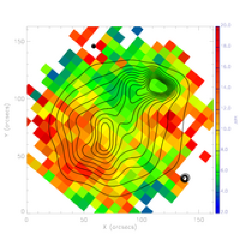
Figure 20: Temperature map of MS 1054-0321. The cluster field is divided into $21\times 21$ subregions and the MEKAL plasma model is fit to the spectrum extracted from each cell with a fixed abundance of $Z=0.30$. The blank (white) cells represent the region where the model fit is judged to be insignificant. X-ray flux contours are overlaid for reference. The eastern part of the cluster is estimated to be of higher temperature than the western part. There appears to be no shock-heated region between the two X-ray peaks.

This result indicates that there may exist severe temperature variation within the cluster. In order to address the issue further, we constructed the temperature map of the cluster as follows. We divided the cluster field $160\arcsec\times 160\arcsec$ into $21\times 21$ subregions and extracted a spectrum for each subregion after applying the RMF and the ARF corrections as above. To prevent the poor photon statistics from leading to a spurious temperature, we not only allowed an ample overlapping between subregions, but also the resulting spectrum is ensured to contain at least 50 counts per spectral bin. Then, the spectrum is fit to the MEKAL plasma model with a fixed abundance of $Z=0.30$. We present this temperature map in Figure 20. We examined the fitting result for each grid and rejected the resulting temperature if the fit appears to be insignificant because of the poor photon statistics. The overall temperature structure is somewhat similar to the hardness ratio map (Jeltema et al. 2001), but this temperature map derived from the direct spectral fitting enables a quantitative comparison between different regions. We verified that the temperature estimation based on this map is consistent with the result summarized in Table 3.

Cosmological simulations of the intracluster medium (e.g., Schindler & Mueller 1993; Ricker 1998; Takizawa 1999; Ricker & Sarazin 2001) have demonstrated that there develop shock-heated regions between sub-clusters approaching each other, stretched perpendicular to the merging axis. However, the temperature structure of MS 1054-0321 does not indicate such a feature between the centers of the two X-ray peaks. Instead, we note that the large scale temperature variation is reminiscent of the quadrupole temperature structure (i.e., two high-temperature regions propagating in opposite directions along the merger axis) observed at the post-merger stage in numerical simulations. The disrupted appearance and the flat surface brightness profile (see §4.3) of the central X-ray peak are also consistent with this conjecture that the central X-ray peak might have gone through a recent merger. We discuss a possible scenario in association with the absence of the eastern X-ray peak in §5.7.

4.3 Isothermal Beta Description of the Cluster

The complicated substructure of the cluster makes it challenging to fit the surface brightness profile to an isothermal beta model, which assumes a spherical symmetry, and the attempts often lead to physically unreasonable parameters.

We created an exposure-corrected image by binning 0.8-7 keV photons with $\sim 2\arcsec\times 2\arcsec$ pixels. Initially, we attempted to model the surface brightness profile of the cluster with a superposition of two isothermal beta profiles. However, as noted by Jeltema et al. (2001), the central X-ray peak requires a large beta index ($\beta\sim 1.3$) whereas the western X-ray peak profile is nicely fit with a beta index of $\beta=0.58\pm 0.15$ and a core radius of $r_{c}=17\arcsec\pm 7\arcsec$. We suspect that the large beta index for the central X-ray peak originates from the flat core, most probably due to recent merger activity. Therefore, the mass calculation of the cluster from this approach is flawed and subject to overestimation.

Instead, we decided to fit a single isothermal beta profile to the entire cluster, excluding the complicated inner substructure. Numerical simulations (e.g., Rowley et al. 2004) show that the merger of the global ICM precedes that of the core merger, which tends to maintain the bulk motion up to the late stage of the event. If we assume MS 1054-0321 is undergoing a major merger between the western and central clumps, and also the central clump has already suffered a recent merger, we argue that our fitting a isothermal beta profile to the outer region of the X-ray profile minimizes the artifact arising from this hypothesized merger activity.

To this end, the binned X-ray image was first fitted to a single two-dimensional isothermal beta model to determine the centroid that maximizes the azimuthal symmetry. After the optimal centroid was determined at $\alpha\simeq 10^{h}56^{m}58^{s}.7$ and $\delta\simeq-03\arcdeg 37\arcmin 36\arcsec.1$, we constructed an azimuthally averaged surface brightness profile, which was then fit to one-dimensional isothermal beta model. Because the centroid was placed $\sim 40\arcsec$ apart from both X-ray peaks, we excluded the inner region ($r<45\arcsec$) from the fit, which yielded a core radius of $16\pm 15\arcsec$ and a $\beta$ index of $0.78\pm 0.08$. The uncertainties are computed with both parameters allowed to vary.

The $\beta_{spec}$ index or specific energy ratio of the dark matter and ICM is defined as

$$\beta_{spec}=\frac{\mu m_{p}\sigma^{2}}{k_{B}T},$$ (11)

and we can predict a value of $\beta_{spec}\simeq 0.9$ using $T=8.9$ keV and $\sigma=1150\mbox{km}~{}\mbox{s}^{-1}$ for the entire cluster. If we adopt the correction factor ($\beta_{spec}=(1.25\pm 0.1)\beta_{fit}$) from Bahcall & Lubin (1994), the $\beta_{fit}$ is estimated to be $\sim 0.73$, which nicely matches the measured $\beta$ index of $0.78\pm 0.08$ above.

We show the radial surface brightness profile from the X-ray emission in Figure21 with the best-fit isothermal beta profile (dashed line). When the inner region is not excluded, the resulting isothermal beta profile (dotted line) must be described with a physically unrealistic value of $\beta\simeq 1.66$ (i.e., much hotter dark matter than the ICM) and $r_{c}\simeq 81.7\arcsec$.

4.4 X-ray Mass Estimation

One can estimate the total gravitating mass of the cluster once the core radius, the $\beta$ index, and the temperature are determined (Evrard et al. 1996):

$$M(r)=1.13\times 10^{14}\beta\left(\frac{T}{\mbox{keV}}\right)\left(\frac{r}{\mbox{Mpc}}\right)\frac{(r/r_{c})^{2}}{1+(r/r_{c})^{2}}M_{\sun},$$ (12)

where $r_{c}$ is the core radius and the mean molecular weight of the gas is assumed to be 0.59 times the proton mass.

Equation 12 yields a total mass of the cluster within a spherical volume at $r$ and therefore it is not straightforward to compare this X-ray mass with the weak-lensing estimation, which typically gives an aperture mass inside a cylinder. However, because equation 12 already assumes a spherical symmetry, one can also estimate an analogous projected X-ray mass without any loss of generality. We present a brief derivation of an analytic expression for the X-ray aperture mass as follows.

After converting equation 12 to an expression for a mass density $\rho(r)$, we can integrate the result along the line of sight to obtain the following surface mass density:

$$\Sigma(r)=2.83\times 10^{13}\frac{\beta T}{r_{c}}\left(1+\left(\frac{r}{r_{c}}\right)^{2}\right)^{-3/2}\left(2+\left(\frac{r}{r_{c}}\right)^{2}\right)M_{\sun}$$ (13)

This result was also derived by Clowe, Luppino, & Kaiser (2003) in their comparison of weak-lensing surface mass density with X-ray measurements. The surface mass density can be now integrated from the cluster center to the aperture radius $r$:

$$M_{ap}(r)=2\pi\int_{0}^{r}r^{\prime}\Sigma(r^{\prime})dr^{\prime}=1.78\times 10^{14}\beta\left(\frac{T}{\mbox{keV}}\right)\left(\frac{r}{\mbox{Mpc}}\right)\frac{r/r_{c}}{\sqrt{1+(r/r_{c})^{2}}}M_{\sun},$$ (14)

where again $r$ and $T$ must be given in units of Mpc and keV, respectively.

Using the cluster temperature and the surface brightness profile determined in §4.2 and 4.3, we estimate the projected mass of the cluster within 1 Mpc aperture radius to be $(1.2\pm 0.2)\times 10^{15}M_{\sun}$. This mass is consistent with our parameter-free weak-lensing estimation. In §5.1 we present a detailed comparison of the X-ray mass profile with the weak-lensing result.

5 DISCUSSION

5.1 X-ray Mass versus Lensing Mass

In weak-lensing analysis, the largest uncertainty is introduced when the tangential shear is fit to a particular mass profile in order to constrain $\kappa$ in a certain annulus. The accuracy in determining $\kappa$ for a specified area depends on the conformity of the cluster mass profile to the parameterized model as well as the extent of azimuthal symmetry. Nevertheless, we consider the uncertainty arising from these assumptions to be small for the current analysis because, in spite of the apparent substructure, the mass profile of MS 1054-0321 seems to be well described by the isothermal profile out to the field boundary at least in an azimuthally averaged sense. In addition, $\kappa$ is expected to be small at the annulus near the field boundary and to approach $\kappa\approx\gamma$ with a minor dependence on the assumed model.

On the other hand, the X-ray mass determination potentially harbors many ambiguities due to the indefiniteness of the assumptions involved. The hypothesis that the system is in hydrodynamic equilibrium is often questionable especially in high-redshift clusters where the clusters appear to be still in their forming stage. Besides, many of these high-redshift clusters possess filamentary structure that makes it difficult to use equation 12 or 14, which necessitates an assumption of a spherically symmetric mass distribution. In addition, the accurate measurement of the X-ray structural parameters (i.e., the determination of the core radius and $\beta$ index) is a challenging task, especially for high-redshift clusters where the cosmological surface brightness dimming reduces the photon statistics substantially.

We compare a variety of the mass profiles of MS 1054-0321 in Figure 22. The X-ray mass profiles are computed using equation 14 for different isothermal beta model parameters. First, note that the X-ray mass profile for the parameters determined in § 4.3 ($\beta=0.78$ and $r_{c}=16\arcsec$) maintains a consistency with the weak-lensing mass profile.

A blind isothermal beta profile fitting gives unrealistically large values for the beta ($\sim 1.66$) and the core radius ($\sim 81.7\arcsec$) of MS 1054-0321 as already mentioned in §4.3. The resulting aperture mass at $r=1$ Mpc radius would also become unacceptably huge ($\sim 2.3\times 10^{15}M_{\sun}$). Jeltema et al. (2001) obtained a core radius of $\sim 1.1\arcmin$ when the beta is frozen to unity. These two parameters along with their temperature measurement of $\sim 10.4$ keV suggest a total projected mass of $M(r<1~{}\mbox{Mpc})=\sim 1.7\times 10^{15}M_{\sun}$, which is still larger than our X-ray estimate of $M(r<1~{}\mbox{Mpc})=(1.2\pm 0.2)\times 10^{15}M_{\sun}$. However, we note that the virial mass that Jeltema et al. (2001) computed from the mass-temperature scaling relation (Evrard et al. 1996; Arnaud & Evrard 1999) is similar to our result and the comparison is presented in §5.4.

Although it is encouraging to observe a nice concordance between the X-ray and weak-lensing masses in this particular study, we do not expect that there exists a general agreement for other clusters. Mainly, we attribute the reconciliation of the mass properties in the current study to the excellent conformity of the large scale gas and mass profiles of MS 1054-0321 to that of the isothermal model (i.e., $\rho_{DM}=(1+(r/r_{c}))^{-3/2}$ and $\rho_{ICM}=\rho_{DM}^{\beta}$) out to a large distance from the cluster center despite the apparent temperature variation and cluster substructure. The current method of X-ray mass estimation is limited by the assumption of the isothermality of the cluster profile. Accordingly, the X-ray mass estimation is not always guaranteed to lead to an unbiased result at large radii where the extrapolation of the X-ray profile determined within a small aperture is often problematic. For example, although J05 obtained a weak-lensing mass similar to the X-ray result at small radii for CL 0152-1357 (a difference of $\sim 10$% at $\sim 50\arcsec$), the discrepancy increases continuously toward the field edge because the actual cluster mass profile determined from weak-lensing rises more slowly than the isothermal sphere at large radii, favoring an NFW description.

5.2 Uncertainties of Gravitational Lensing Mass Due to the Cosmic Shear

The gravitational lensing signal is sensitive to all matter along the line of sight. As a result, the shape of a background galaxy is distorted not only by the cluster mass, but also by the background large scale structure in front of and behind the cluster. In the general application of weak-lensing to cluster mass estimation, the cluster is assumed to be the dominant source of signal and the contribution from this cosmic structure is often neglected. Such lack of concern for the background structure can be justified in many situations where the statistical errors resulting from the discrete sampling of the signal overwhelms the uncertainties caused by the large scale structure. However, in our current ACS analysis, the unprecedentedly high number density of source galaxies reduces the measurement errors substantially, making other sources of errors more important.

In this subsection, we assess the effect of the large scale density field in our mass estimation of MS 1054-0321 following the formalism of Schneider et al. (1998) and Hoekstra (2001, H01 hereafter) (see also Kaiser 1992;1998 for the original derivations of many useful equations). The variance of the aperture mass due to the large scale density fluctuation is given by:

$$\left<M_{AP}(\theta)^{2}\right>=2\pi\int_{0}^{\infty}\mbox{d}s~{}P_{\kappa}(s)I(s,\theta)^{2},$$ (15)

where $P_{\kappa}$ is the projected power spectrum defined as:

$$P_{\kappa}(s)=\frac{9}{4}\left(\frac{H_{0}}{c}\right)^{4}\Omega_{M}^{2}\int_{0}^{w_{H}}\mbox{d}w\frac{g^{2}(w)}{a^{2}(w)}P\left(\frac{s}{f_{K}(w)};w\right)$$ (16)

and $I(s,\theta)$ is a filter function dependent on the mass estimation method. The form of the functions for the SIS model and the aperture mass densitometry ($\zeta$-statistic) can be found in H01. In equation 16, $g(w)$ is a source-averaged angular diameter distance ratio $D_{ls}/D_{s}$, $a(w)$ is the scale factor, and $f_{K}(w)$ is the comoving angular diameter distance. We computed $g(w)$ using the redshift distribution obtained from the UDF after applying the same source selection criteria to the UDF catalog. In the evaluation of the projected power spectrum (eqn. 16), we first constructed the non-linear power spectrum (Peacock & Dodds 1996) for the current WMAP cosmology and then integrated it out to the comoving distance to horizon $w_{H}$.

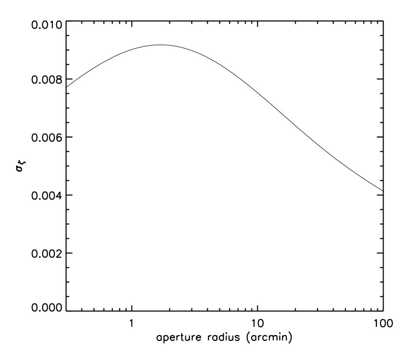
Figure 23: Predicted uncertainties in the measurement of the Einstein radius from the SIS fit (left panel) and the aperture mass densitometry (right panel).

We show the predicted uncertainties in the estimate of the Einstein radius from the SIS fit and the aperture mass densitometry for our source redshift distribution in Figure 23. The overall shape of the aperture-dependent variation and the magnitude of the predicted uncertainties are similar to those estimated by Schneider et al. (1998) and H01. At 1 Mpc ($\sim 132\arcsec$), we predict $\sigma_{\theta_{E}}\simeq 0.74\arcsec$ and $\sigma_{\zeta}\simeq 9\times 10^{-3}$ for the SIS fit and the aperture mass densitometry, respectively, due to the cosmic shear effect. The uncertainty of the best-fit SIS Einstein radius is only marginally increased from $\theta_{E}=11\arcsec.1\pm 1.\arcsec 0$ to $\theta_{E}=11\arcsec.1\pm 1.\arcsec 2$. On the other hand, the effect is relatively large for the aperture mass densitometry. Assuming that $\sigma_{\theta_{E}}$ and $\sigma_{\zeta}$ are correlated, we can estimate the upper limit on the uncertainty for the aperture mass densitometry to be $\sigma_{\bar{\kappa}}\simeq 0.012$. This value of $\sigma_{\bar{\kappa}}$ due to the cosmic shear introduces an additional $\sim 14$% error to the total cluster mass estimation at 1 Mpc, yielding $M(r<1\mbox{Mpc})=(1.02\pm 0.15)\times 10^{15}M_{\sun}$ (adding the statistical error and the cosmic shear effect in quadrature).

The brief analysis above demonstrates that the cosmic shear effect is a significant factor in the total error budget of the cluster mass estimate. In general, the uncertainty due to the effect increases as we probe into higher redshift regimes. However, as indicated by H01, the fractional uncertainty ($\left<\kappa_{cs}\right>^{1/2}/\left<\kappa\right>$ increases only moderately with cluster redshift for rich clusters (e.g., $\sigma=1000\mbox{km}~{}\mbox{s}^{-1}$ ) if we choose faint (e.g., $20<R<26$) source population. In the current analysis, the high-resolution of the ACS images as well as the thorough knowledge of the instrumental PSF allow us to select the unprecedentedly faint ($24<z_{850}<28$) galaxies as our sources, minimizing the cosmic shear effect. H01 shows that if the $20<R<24$ (a typical magnitude range for ground-based weak-lensing analysis) galaxies are used instead, the cosmic shear can contribute a nearly 50% uncertainty in the total mass even for a rich cluster at $z\simeq 0.8$.

A promising way to improve the accuracy dramatically in cluster mass estimate yet not attempted in the current analysis is to perform a so-called weak-lensing tomography. When good photometric redshift information for individual source galaxies becomes available in the future, it is possible to separate the cluster lensing signal from the cosmic shear utilizing the differential lensing efficiency.

5.3 Comparison of the Cluster Substructure with HFK00

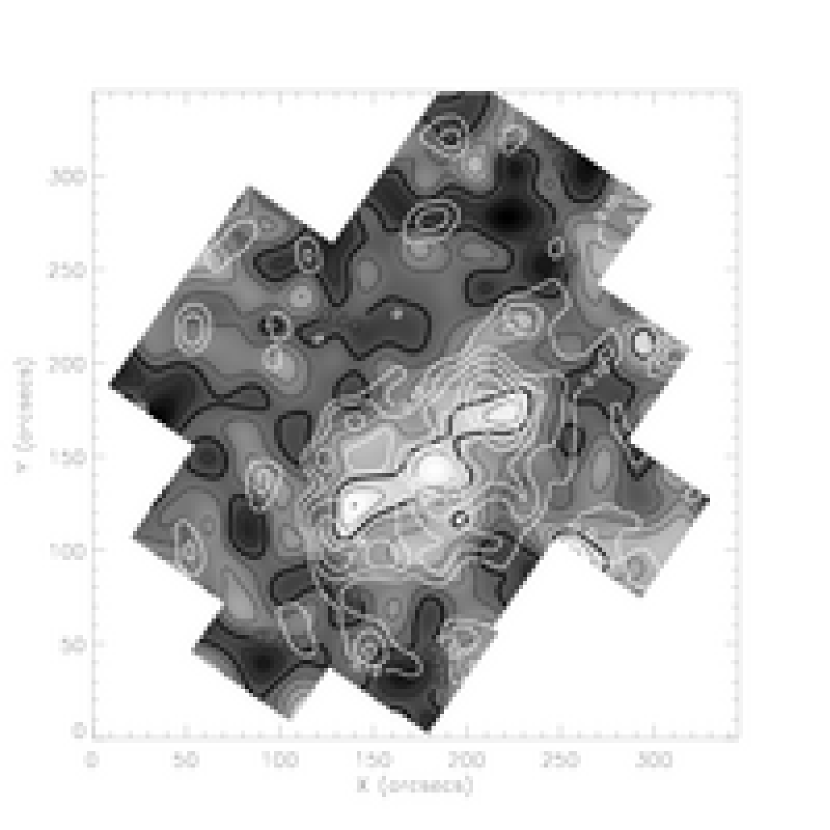
Figure 24: Comparison of the mass reconstruction with the WFPC2 observations (HFK00). The background gray-scale is the mass map presented in HFK00 and the white contours are the current mass reconstruction based on the ACS observations. The alignment between the two sets of contours is only approximate ($\sim 6\arcsec$).

Figure 24 shows our mass reconstruction contours on top of the HFK00 result. The alignment between the two sets of the contours is only approximate ( $\sim 6\arcsec$). The main structure of MS 1054-0321 characterized by the three major clumps is obvious in both results. The central and western mass clumps in HFK00 are in good spatial agreement with our results. However, we note that their eastern clump is displaced to the west by $\sim 20\arcsec$. In our mass reconstruction the eastern clump is further resolved into two or possibly three smaller mass peaks, in better spatial agreement with the cluster optical lights (see Figure 15).

There are some indications that the minor peaks labeled as M1-4 in Figure 16 are also present in HFK00 mass map, but the significance of their detections appears to be marginal and the locations have greater offsets from the corresponding luminosity clumps.

5.4 Virial Radius

There exist different definitions for a virial radius in the literature, mostly due to the discrepant definitions of a characteristic density of a halo. We define the virial radius of the cluster as a radius where a mean density inside the spherical volume becomes 200 times the critical density at the redshift of the cluster. Although spherical collapse simulations suggest different criteria for a virialized halo depending on the cosmological parameters and normalization, we adopt this conventional definition to ensure that a straightforward comparison can be made to previous work.

If the isothermal beta model (Eqn. 12) is used, the X-ray measurements predict a virial radius of $1.7\pm 0.2$ Mpc ($\sim 224\arcsec$) for MS 1054-0321. A similar value of $1.5\pm 0.1$ Mpc is obtained if the weak-lensing mass from the SIS fit result is extrapolated assuming spherical symmetry. The corresponding virial masses $within$ $the$ $sphere$, then, become $(1.2\pm 0.2)\times 10^{15}M_{\sun}$ and $(1.1\pm 0.1)\times 10^{15}M_{\sun}$ from the X-ray and weak-lensing analyses, respectively.

Jeltema et al. (2001) quoted $M_{200}=6.2_{-1.3}^{+1.6}\times 10^{14}M_{\sun}$ within $r=0.76$ Mpc from the mass-temperature scaling relation (Evrard et al. 1996; Arnaud & Evrard 1999) in the $(\Omega_{M},\Omega_{\Lambda},h)=(1,0,1)$ universe. Using the same cosmological parameters, our X-ray virial mass is transformed to a similar value of $M(r<0.74$ Mpc)=$(5.8\pm 0.7)\times 10^{14}M_{\sun}$ from equation 12. Although Jeltema et al. (2001) claimed that their mass estimate is lower than the HFK00 weak-lensing mass by $\sim 38$% (compared at the same radius of r=0.76 $h_{100}$ Mpc in the above $\Omega_{M}=1$ cosmology), our analysis shows that the two results are consistent with each other (on the contrary, their X-ray mass becomes even slightly higher than the weak-lensing mass) when the projected weak-lensing mass is properly converted to the total cluster mass within a spherical volume.

5.5 Comparison of the Velocity Dispersion and Sunyaev-Zeldovich Analyses

The most recent determination of the velocity dispersion of MS 1054-0321 from the spectroscopic catalog of the cluster members (Tran et al. in prep.) is $1153\pm 80\mbox{km}~{}\mbox{s}^{-1}$. The value is very close to our weak-lensing prediction (§3.6) of $1150_{-51}^{+49}$ km$s^{-1}$ under the SIS assumption The empirical relation between X-ray temperature and velocity dispersion is rather scattered around the theoretical $\sigma\propto T^{1/2}$ line. Adopting ($\sigma_{v}/\mbox{km~{}s}^{-1})=10^{2.57\pm 0.13}(kT/\mbox{keV})^{0.59\pm 0.14}$ (Wu et al. 1998), we obtain $\sigma_{v}=1349_{-340}^{+461}\mbox{km}\mbox{s}^{-1}$. If we use the theoretical relation instead assuming energy equi-partition, the X-ray temperature of $T=8.9_{-0.8}^{+1.0}$ keV corresponds to $\sigma_{v}=1202_{-55}^{+66}\mbox{km s}^{-1}$.

From Sunyaev-Zeldovich (SZ) imaging of the cluster, Joy et al. (2001) estimated a temperature of $10.4_{-2.0}^{+5.0}$ keV and a projected mass ($r<94\arcsec$) of $(4.6\pm 0.8)\times 10^{14}M_{\sun}$ (under the $(\Omega_{M},\Omega_{\Lambda},h_{100})=(0.3,0.7,1)$ cosmology). The conversion of our weak-lensing result to their cosmological parameters yields a projected mass of $(4.9\pm 0.3)\times 10^{14}M_{\sun}$ ($r<94\arcsec$), which is in good agreement with the SZ estimation.

It may be considered surprising to observe the converging results between weak-lensing and other various analyses above especially for this high-redshift cluster. One interpretation of these impressive agreements is that the dynamical structure of MS 1054-0321 may already have matured even at $z\sim 0.83$ to the extent that at least the azimuthally averaged properties do not depart greatly from that of a relaxed cluster in spite of the elongated appearance of the cluster galaxy distribution. It will be interesting to examine in future investigations how critical the role of the ICM is in the global virialization of the cluster.

5.6 Offsets between Galaxies, ICM, and Dark Matter

In §3.8, we discussed the cluster substructure revealed by the weak-lensing mass reconstruction in comparison with the cluster luminosity distribution. A careful examination of the mass/light overlay (Figure 15) shows that there present some offsets between the mass and luminosity centroids. In order to investigate the statistical significance of these offsets, we ran a 5000 bootstrap resampling of background galaxies and measured the centroid of the mass peaks from each realization. We found that only the central and western mass clumps possess statistically significant offsets with respect to the corresponding luminosity peaks. Figure 26 demonstrates that both luminosity centers are outside the 99% circle of the mass peak centroid distribution.

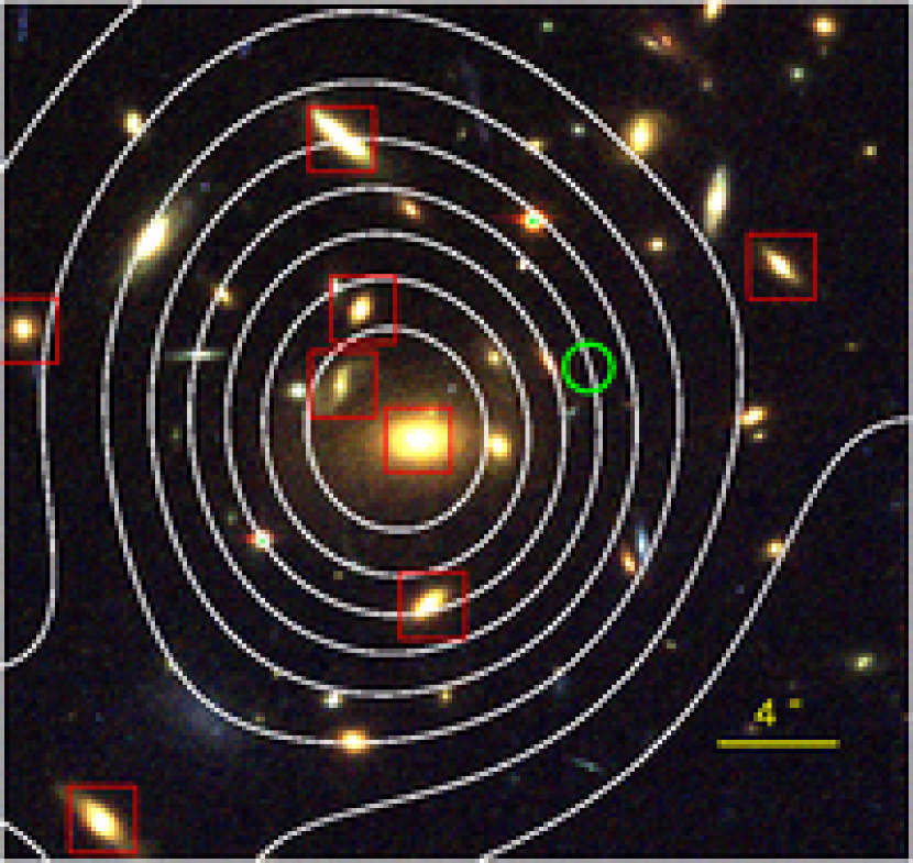
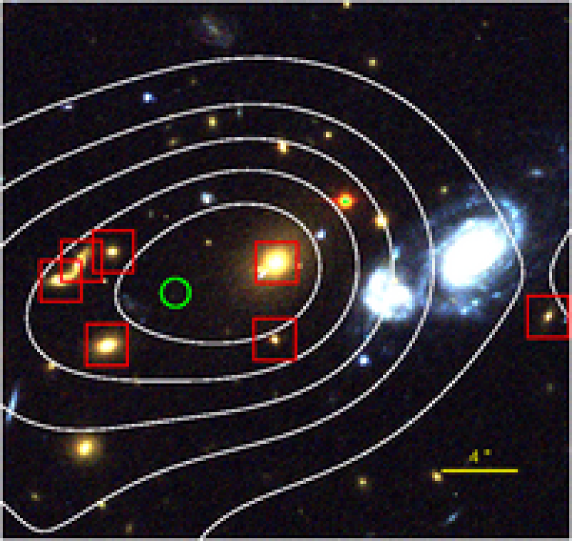
Figure 27: The luminosity contours overlaid on the enlarged color images of the central (left) and western (right) mass clumps. The luminosity contours are drawn in white, and red squares are placed on the spectroscopically confirmed members. We also mark the mass centroids with green circles. It is apparent that the luminosity centroids are mostly influenced by the BCGs. The smoothed central luminosity peak has its centroid only $\sim 1\arcsec$ apart from the location of the BCG. The offset is $\sim 2\arcsec$ for the western luminosity clump.

Another important question in this mass-light centroid comparison is whether the above luminosity centroids are fair locations to compare with the mass centroids. If the luminosity centroids are severely affected by the incompleteness and/or the smoothing kernel size, we may also need to consider the resulting uncertainties in our analysis. We present the overlay of the detailed luminosity contours of the central and western clumps on top of their color images in Figure 27. The luminosity contours are drawn in white, and red squares are placed on the spectroscopically confirmed members. We also mark the mass centroids with green circles. It is apparent that the luminosity centroids are mostly influenced by the BCGs. The smoothed central luminosity peak has its centroid only $\sim 1\arcsec$ apart from the location of the BCG. The offset is $\sim 2\arcsec$ for the western luminosity clump. We remember that the luminosity map is smoothed with a FWHM$\simeq 14\arcsec$ Gaussian kernel whereas we used a FWHM$\sim 10\arcsec$ kernel for the smoothing of the mass map. Considering an additional smoothing ( $\sim 10\arcsec$) implicitly done in averaging source ellipcities before the mass reconstruction, we estimate that the FWHM of $14\arcsec$ for the luminosity smoothing is a proper kernel size to ensure a comparable smoothing scale (dispersion by finite sizes of galaxies can be neglected because the FWHM$\simeq 14\arcsec$ Gaussian kernel is so dominant). If one argues that a smaller kernel must have been used in smoothing the light distribution in order to secure a fair comparison, it is easy to ascertain that a smaller kernel will only shift the luminosity centroids toward the BCGs, enlarging the offset between the luminosity and mass centroids. Alternatively, if one prefers a larger kernel for a luminosity map, we find that increasing kernel size reduces the offsets between the luminosity and mass centroids, which, nevertheless, still remain significant at a 2$\sigma$ level ($\gtrsim 4\arcsec$ and $\gtrsim 2.5\arcsec$ for the central and western clumps, respectively) up to a FWHM$\sim 20\arcsec$. Of course, for this large kernel (FWHM$\sim 20\arcsec$), the contribution from the cluster members absent from the spectroscopic catalog may become relatively important. However, the examination of the distribution of unconfirmed cluster candidates around the BCGs does not convince us that this will modify the significance of the mass/luminosity offsets substantially.

Given the above argument that the luminosity centroids stay close to the BCGs for the reasonable values of the smoothing kernel, we list the following possibilities as causes of the observed offsets:

• noises from discrete sampling of background galaxies,

• systematics shifts due to foreground masses, and

• real features reflecting different hydrodynamical properties of individual cluster constituents.

1. Noises from discrete sampling of background galaxies. In general, the finite sampling of the background galaxies whose spatial distribution is not uniform scatters the centroids of mass reconstruction from their true positions. The stability of the centroids are mainly determined by the strength of the lensing signal as well as the number density of available source galaxies. As we found that the signal around the two mass peaks is very strong and the number density of sources is unprecedentedly high ($\sim 154~{}\mbox{arcmin}^{-2}$), the uncertainty of the centroids are expected to be small. One of the most useful tests to assess the errors is a bootstrap resampling of background galaxies discussed above. The result is consistent with our intuition that the more pronounced peak (the western mass clump) has a smaller dispersion than the weaker one (the central mass clump). Because both luminosity centroids are significantly outside the 99% enclosing circle of the corresponding mass centroids (Figure 26), it is very unlikely that the observed mass/light offsets originate from the noises.

2. Systematic shifts due to foreground masses. As light rays are perturbed by any objects between the observer and source, we cannot preclude the possibility that there might exist some foreground/background masses responsible for the mass centroids. In §5.2, we have estimated the uncertainties in our cluster mass due to the presence of other large scale structures. In particular, lower redshift foreground objects can work as more efficient lens and measurably alter the mass map even if their masses are not as significant as that of MS 1054-3021. One of the most unambiguous tests is to perform a so-called weak-lensing tomography, which can, in principle, separate the cluster mass from the dynamically uncorrelated background/foreground structures. The technique, however, requires us to obtain a good photometric redshift knowledge of individual sources and thus can become practical only in the future.

Nevertheless, without this sophisticated check, it is still possible to discuss the effects of these possible interlopers by scrutinizing our mass map. If the foreground masses are to greatly affect the centroids of the cluster mass clumps, they must have a rather peaked distribution whose width (e.g., FWHM) is less than or comparable to those of the cluster mass peaks. (if the foreground mass distributions are much smoother than the characteristic scale of the mass peaks, they cannot shift the cluster centroids by the large amount as observed in our case). Besides, the peaked foreground mass must be located very close to the mass centroids of the cluster perhaps within a smoothing kernel (FWHM$\simeq 10\arcsec$) in order to shift the centroids. Otherwise, we suspect that they should reveal themselves as separate peaks in our high-resolution mass reconstruction. Finally, we analyze the spectroscopic catalog of the cluster field to examine if there is any concentration of foreground galaxies. Out of 325 objects whose redshifts are known, about $150$ galaxies are found to lie foreground. Although the spectroscopic survey is incomplete and still in progress (Tran et al. in preparation), we found no significant foreground groups near the two cluster mass centroids.

3. Real features reflecting different hydrodynamical properties of individual cluster constituents. There is a growing list of X-ray clusters whose intracluster gas might have been swept back behind the corresponding cluster galaxies possibly due to the ram pressure (e.g., Markevitch et al. 2002; Maughan et al. 2003; Scharf et al. 2004). Although the discovery is rather recent, the ICM-galaxy offsets seem to be acquiring increasing observational supports. On the other hand, the mass-galaxy offsets have not been reported in any other investigations yet except in our previous weak-lensing analysis of CL 0152-1357 (J05). Markevitch et al. (2004) suggest that one can use the mass-galaxy displacements to constrain the collisional cross-section of the dark matter particles because, if cluster galaxies are to suffer any deceleration from the dark matter collisions, the cluster galaxies should be hauled by the dominant dark matter potential well and appear to be displaced away from the merging direction.

Alternatively, one can also propose a different scenario wherein the dark matter particles are purely collisionless, but collisional properties of the cluster galaxies are not negligible. This is against a conventional yet disputable belief that galaxies are effectively collisionless. Detailed numerical simulations must be followed in order to estimate whether the effect is measurable and can lead to such an observed offset.

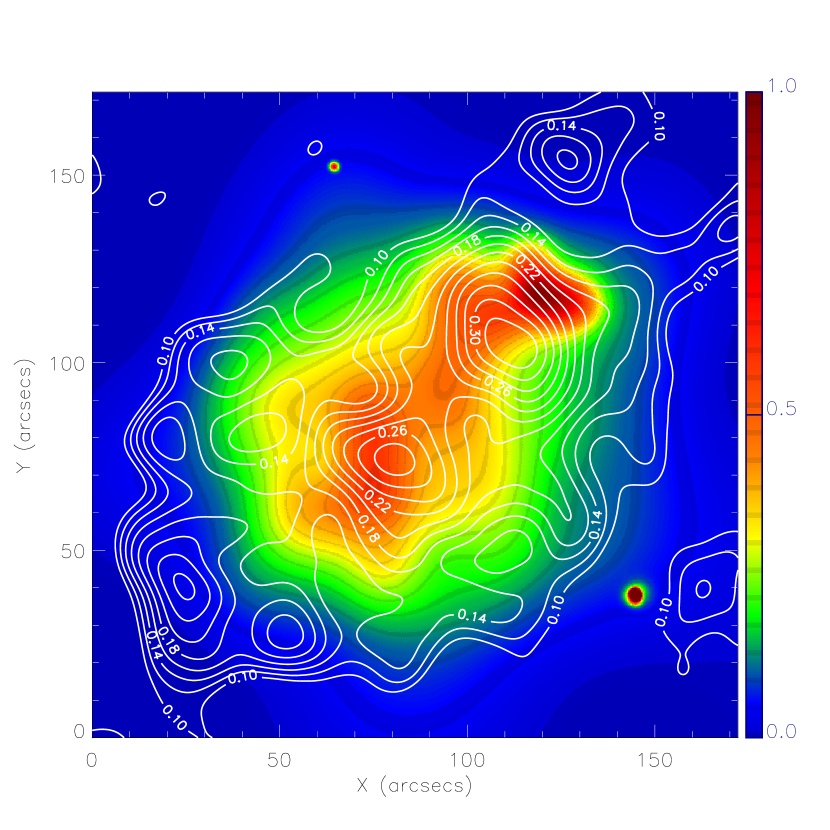
Figure 28: Mass reconstruction on top of the X-ray map. The eastern mass clump is not detected in the $Chandra$ X-ray observation. Under the hypothesis of a merger, the central and western dark matter clumps seem to be moving ahead of the corresponding X-ray peaks.

As argued by Clowe et al. (2004), the mass-ICM offset can be used to support the existence of dark matter. There have been some attempts to explain the “missing matter”, particularly in clusters of galaxies, in the context of the Modified Newtonian dynamics (MOND; Milgrom 1983). The MOND theory has been partly successful in describing the observed velocity dispersions of galaxy clusters as well as rotation curves of spiral galaxies without inclusion of dark matter by modifying the Newtonian gravity so that the inertia mass of a particle is decreased in the limit of low accelerations (e.g., McGaugh & de Blok 1998; Sanders 2003; Milgrom & Sanders 2003). Recently, Bekenstein (2004) has proposed a relativistic extension of MOND, which now predicts definite gravitational lensing. If we view the cluster in this MOND paradigm, the centroids of the mass clumps are expected to lie on top of the X-ray peaks, which trace the dominant baryonic component of the cluster. However, our lensing analysis (Figure 28) shows with high significance that the locations of these X-ray peaks are not where the dominant cluster mass is concentrated. A similar trend is observed in the weak-lensing analysis of the interacting cluster 1E 0657-558 (Clowe et al. 2004). The 1E 0657-558 cluster shows not only the dramatic bow-shock from the X-ray emission, but also the two dark matter clumps conspicuously offset from the corresponding X-ray peaks.

5.7 Absence of the Eastern X-ray Peak

As is clear in Figure 28, the Chandra observation does not detect any X-ray excess over the eastern region of MS 1054-0321 where the weak-lensing and luminosity map reveal distinct mass concentrations. The absence of this third weak lensing peak in the X-ray observation was first observed by Clowe et al. (2000) in the comparison of the ROSAT/HRI X-ray analysis with their Keck weak-lensing result.

Jeltema et al. (2001) proposed two possibilities regarding the discrepancy: immaturity of the eastern clump or an artifact of noisy mass reconstruction caused by sub-optimal smoothing (Marshall 2002). The high significance of the substructure detected by the unprecedentedly high number density of source galaxies using $HST$/ACS images immediately rules out the second possibility. Besides, the consistency of our weak-lensing substructure with the result of HFK00 despite the different selection and measurement of background galaxies, as well as the overdensity of the spectroscopically confirmed cluster galaxies at the eastern mass clump evidence that this eastern substructure is real.

The first scenario that the third clump has not fully developed into an X-ray system is an interesting possibility, considering the extremely high temperature ($10^{7}-10^{8}\mbox{K}{\arcdeg}$) required for thermal Bremsstrahlung radiation. As seen by the cluster light distribution, the cluster galaxies in this region appear to be less concentrated and luminous than in the other two clumps. The weak-lensing mass in the eastern clump is also somewhat lower ($\sim 70$% of the western mass clump).

However, the predicted gas temperature derived from an empirical $\sigma-T$ relation (e.g., Wu et al. 1998) is $3.3\pm 0.6$ keV after the projected mass ($(9.3\pm 1.5)\times 10^{13}M_{\sun}$ within $30\arcsec$) is converted to the velocity dispersion ($747\pm 65\mbox{km}~{}\mbox{s}^{-1}$) under SIS assumption. Hence, even considering the scattered $\sigma-T$ relation and the surface brightness dimming at $z\sim 0.83$, it is difficult to justify the lack of the X-ray emission exclusively by the low temperature of the subcluster. The western Lynx cluster RXJ 0848+4453 at z=1.27 (Stanford et al. 2001) has even a lower X-ray temperature of $T<2$ keV with a weak-lensing mass of $M(<0.5$ Mpc$)\sim 2\times 10^{14}$ (M. Jee et al., in preparation), but the $Chandra$ X-ray image confirms the presence of the X-ray emission associated with the cluster.

An alternative scenario can be envisaged, in which most of the intracluster gas of the eastern clump has been stripped while passing through the dense region of the central substructure. If we imagine that clump E traveled from the southwest of clump C and passed through it possibly with an off-center collision, clump E would then lose a significant fraction of its ICM, or most of its ICM would become bound to that of clump C, leaving a double-peaked structure as is hinted in our current X-ray contours. This post-merger picture is partly supported by the temperature structure of the cluster (Figure 20) showing that the cluster temperature is rapidly rising in opposite directions from the central X-ray peak to the east and the west as mentioned in §4.2. A similar temperature structure is observed in numerical simulations of cluster ICM and particularly Takizawa (2000) demonstrated in his off-center merger simulation that double-peak features in X-ray emission would survive even after the most violent epoch.

The flat inner region (possibly with double core) of the central X-ray peak yields a $\beta$ index that is greater than unity (§ 4.3) when the azimuthally averaged radial profile is fit to the isothermal beta profile. The large $\beta$ value indicates that the ICM of the region might have been distorted due to the recent merger. The numerical simulation by Takizawa (1999) showed that the specific energy ratio of dark matter and the ICM (eqn. 11) remains greater than unity even in the late stage of the merger event. In addition, the rather scattered distribution of cluster galaxies and dark matter in the eastern region might be associated with the gravitational disruption during this hypothesized pass-through.

Because the current resolution of the temperature map is not limited by the optical resolution, but by the poor photon statistics, a longer exposure X-ray observation of MS 1054-0321 will provide more significant details of the thermodynamical structure out to a larger distance from the cluster center and enable us to test this merger hypothesis further.

5.8 Formation Sequence of MS 1054-0321

Since more massive clusters are believed to have collapsed earlier within a hierarchical structure formation paradigm, it is natural to conjecture that these clusters are also more likely to possess higher $M/L_{B}$ values resulting from their older stellar population (Bahcall & Comerford 2002). Compared with CL 0152-1357 (J05) at a similar redshift of z=0.84, MS 1054-0321 has both higher mass and $M/L_{B}$ within 1 Mpc, consistent with the hypothesis that $M/L_{B}$ values increase with cluster richness.

If MS 1054-03 is indeed being formed by the hierarchical infall of the smaller mass clumps, which have collapsed at different times, we can also extend and apply the above argument to the wide range of $M/L_{B}$ ratios of the substructure. Table 1 shows that the $M/L_{B}$ ratios of the cluster main clumps (E, C, and W) increase with their masses (we do not include the minor clumps (M1-4) in the discussion because of the reasons explained in §3.8). If this trend is interpreted as an indication of the formation time sequence, the highest $M/L_{B}$ value of the western clump may signify the earliest formation epoch of the substructure. This speculation is further supported by the cluster metallicty distribution (Table 3;§4.2). The western X-ray peak has higher metal abundance than the other X-ray peak, which suggests that the stellar contents of the galaxies associated with the western X-ray peak might be older.

6 SUMMARY AND CONCLUSIONS

We have presented our $HST$/ACS weak-lensing and $Chandra$ X-ray analysis of MS 1054, guided with an extensive spectroscopic survey data of the cluster field. The weak-lensing mass reconstruction, empowered by the superb resolution and sensitivity of ACS, not only confirms the existence of the three dominant mass clumps reported by HFK00, but also further resolves the cluster substructure in unprecedented detail.

In the $Chandra$ X-ray analysis, we took care to properly compensate for the low-energy DQE degradation of the instrument. As demonstrated by a variety of different results in the literature, the temperature measurement is sensitive to the applied correction. In addition to the low-energy DQE correction, it has been realized that even a mild background flare can bias the temperature measurement by a few keV. Utilizing the newly available calibration data and recommendation from CIAO, we obtained $T=8.9_{-0.8}^{+1.0}$ keV for the cluster temperature as a whole. As first noted by Jeltema et al. (2001), the western X-ray peak has a lower temperature than the central X-ray peak. In our temperature map, the cluster seems to have a severe temperature variation across the field.

We excluded the central region ($r<45\arcsec$) in our determination of the structural parameter because otherwise the substructure leads to a physically unacceptable condition for a relaxed isothermal beta sphere, where the cluster dark matter possesses a significantly higher temperature than the ICM particles. We found that the isothermal beta description of the cluster with $\beta=0.78\pm 0.08$ and $r_{c}=16\arcsec\pm 15\arcsec$ yields a consistent mass profile with that from weak-lensing.

The comparison of the weak-lensing mass map with the X-ray contours provides an invaluable opportunity to examine how differently these two cluster constituents are distributed within the cluster. The relatively circular distribution of the ICM in contrast to the rather elongated arrangement of cluster galaxies is consistent with the expectation that the ICM has reached a higher degree of virialization than the cluster galaxies and dark matter. On the other hand, the distribution of the cluster dark matter looks somewhat similar to that of the cluster’s optical luminosity.

Apart from the offsets between the two X-ray peaks and the corresponding dark matter clumps, as first observed in our previous study of CL 0152-1357, we note that there present offsets between the dark matter and the cluster galaxy centroids in MS 1054-0321. Through bootstrap resampling experiments,we demonstrate that the offsets between the dark matter and cluster galaxy centroids are statistically significant. We argue that it is unlikely that the observed offsets are mainly caused either by the different smoothing scale of the light map or the incompleteness of the spectroscopic survey catalog. It is possible that any significant foreground mass lying close to the mass peaks can potentially affect the mass centroids. Although we cannot prove with current data that this possibility is completely ruled out using the so-called weak-lensing tomography, the analysis of the current spectroscopic catalog does not support any presence of such foreground groups nearby the mass centroids. In addition, it is hard to imagine that all the four mass peaks in MS 1054-0321 and CL 0152-1357 coincidently possess close neighbors in projection, which all cause the centroids to look shifted toward the hypothesized merging direction. Therefore, we suggest that the observed offsets between the mass and galaxy centroids might reflects the real features, indicative of a merger between the substructures.

The eastern weak-lensing clump is not detected in X-rays, and possible scenarios have been discussed. Because the eastern mass peak was also clearly detected by HFK00 even with a different selection of background galaxies and the overdensity of the cluster galaxy is present at the location, we rule out the possibility that it is an artifact of the mass reconstruction. As the estimated X-ray temperature ($\sim 3.5$ keV) of the unseen eastern clump based on the projected mass is sufficient for thermal bremsstrahlung radiation, it is not clear whether the lack of the detection is entirely due to the immaturity of the subcluster. Alternatively, we suspect that the ICM of the eastern clump might have been substantially stripped off during its merger with the cluster main body. The first indication of this scenario comes from the temperature structure resembling the propagation of the shock-heated region along the merger axis observed in numerical simulations.

If the subcluster had passed through the dense region of the central clump from the southwest, we suspect that it is possible to observe this kind of temperature gradient increasing in opposite directions. Although this interpretation of the temperature map is not unique, the scenario is further supported by the rather anomalous X-ray profile of the central X-ray peak. Even after the western substructure is carefully removed, the remaining structure cannot be well described by an isothermal beta model because the core region is too diffuse. This may suggest that the ICM structure might have been recently disrupted and we are just observing the transient state prior to its returning to relaxed distribution.

ACS was developed under NASA contract NAS5-32865, and this research was supported by NASA grant NAG5-7697. We are grateful for an equipment grant from Sun Microsystems, Inc. We thank the anonymous referee for constructive criticisms and a careful reading of the manuscript.

Figure 2: Magnitude distribution of detected objects in MS 1054-0321 field. Galaxies were detected using the SExtractor program by searching for at least five connected pixels above 1.5 times the sky rms. The detection looks complete down to $\sim 27$th mag in every filter.

Figure 4: Color magnitude diagram. Because of the location of the redshifted 4000Å break, the early-type galaxies are well separated by their $v_{606}-z_{850}$ colors. Square symbols represent the spectroscopically confirmed cluster members.

Figure 5: Cumulative B band luminosity of MS 1054-0321. We used the spectroscopic catalog in conjunction with the tight CM relation of the early-type galaxies for member selection (see text for details). Within 1 Mpc ($\sim 132\arcsec$) the cumulative B band luminosity is estimated to be $\sim 8.2\times 10^{13}L_{B\sun}$.

Figure 6: PSF anisotropy correction for $v_{606}$ image. The length and orientation of each stick represent the magnitude and direction of the ellipticity, respectively. The stick in the centers of a) and b) shows an ellipticity of $\delta=0.1$. The 2$\times$2 parallelograms illustrate the four pointings of WFC. (a) Stars are elongated coherently with a typical ellipticity of $\sim$10%. (b) Rounding kernel reduces the PSF anisotropy remarkably ($\left<\delta^{2}\right>^{1/2}\simeq 0.02$), indicating that our model PSF is an excellent description of the real PSF.

Figure 7: PSF anisotropy removal in the $v_{606}$ image. Diamonds show the initial ellipticities of stars, and plus symbols, the corrected ellipticities after rounding kernel convolution.

Figure 8: Tangential shear for different magnitude samples. Tangential shears are measured for $bright$ (a; $24<z_{850}<26$), $faint$ (b; $24<z_{850}<28$), and $faintest$ (c; $24<z_{850}<30$) source samples. It is found that we can include faint galaxies down to $z_{850}\sim 28$ without diluting the signal.

Figure 9: Tangential shear for different color samples. The $faint$ sample in Figure 8 are further divided into $faint$ $red$ (top panel) and $faint$ $blue$ (bottom panel) subsamples. There exists a clear dependence of the signal strength on background galaxy colors.

Figure 10: Weak-lensing cluster mass estimation. Aperture mass densitometry (open circle with error bars) yields a total aperture mass of $(1.02\pm 0.04)\times 10^{15}M_{\sun}$ within 1 Mpc ($\sim 132\arcsec$), which is in good agreement with the measurement $(1.01\pm 0.04)\times 10^{15}M_{\sun}$ from the rescaled mass map (dotted). At large radii ($r>60\arcsec$), these cluster mass profiles are similar to the SIS estimation (solid) nearly out to the field boundary. The result from the NFW fitting (dashed) predicts a somewhat lower mass ($\sim 12$% at 1 Mpc).

Figure 11: Mass-to-light ratio profile of MS 1054. The cumulative $M/L_{B}$ ratio (circle) continuously increases out to the field limit. The differential $M/L_{B}$ ($\delta M(r)/\delta L_{B}(r)$) plot is computed after smoothing the luminosity profile (Figure 5).

Figure 21: X-ray surface brightness profile. The open circles represent the azimuthally averaged surface brightness. Because of the substructure, the central region ($r<45\arcsec$) was excluded in isothermal beta fitting, yielding $r_{c}=16\arcsec\pm 15\arcsec$ and $\beta=0.78\pm 0.08$ (dashed). If we use all the data points, the fitting requires a physically unrealistic value of $\beta\simeq 1.66$ and $r_{c}\simeq 81.7\arcsec$ (dotted).

Figure 22: Comparison of weak-lensing mass with X-ray results for different isothermal beta parameters. Our adopted X-ray structual parameters ($\beta=0.78$ and $r_{c}=16\arcsec$) provide the mass profile consistent with the weak-lensing result.

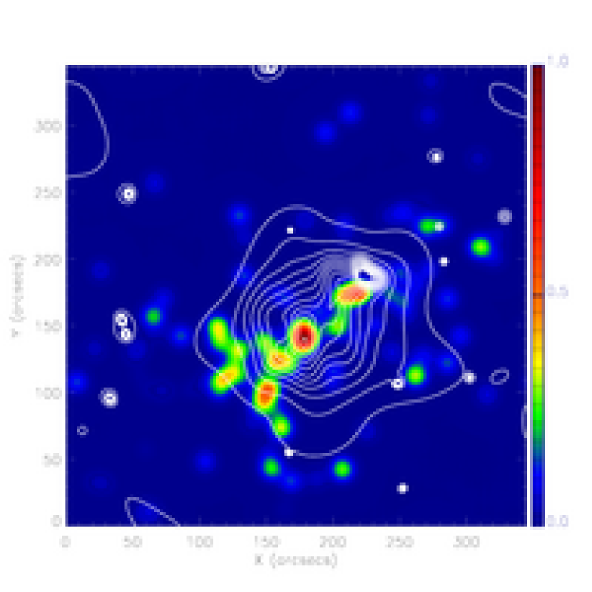
Figure 25: X-ray contours overlaid on the luminosity map. The alignment is precise within $1\arcsec$. The two X-ray peaks are separated further than the corresponding cluster galaxies. The eastern substructure (here shown by the cluster galaxies) is not visible in the X-ray image.

Figure 26: Centroid distribution in 5000 bootstrap resampling of source galaxies. The central mass clump (left panel) has a larger distribution than the western mass clump (right panel), which is consistent with their different masses (thus with different significance). The corresponding luminosity centers are outside the boundary (solid), which encloses 99% of the centroids.

Table 1: PROPERTIES OF THE SUBSTRUCTURES

Clump	Coordinate	Mass ($r<30\arcsec$)	$M/L_{B}$
	(RA,DEC)	($10^{14}M_{\sun}$)	($M_{\sun}/L_{B\sun}$)
W	$10^{h}56^{m}56^{s}.7$,$-03\arcdeg 37\arcmin 43\arcsec.0$	$1.31\pm 0.14$	$219\pm 23$
C	$10^{h}56^{m}59^{s}.7$,$-03\arcdeg 37\arcmin 38\arcsec.4$	$1.23\pm 0.14$	$144\pm 16$
E	$10^{h}57^{m}03^{s}.8$,$-03\arcdeg 37\arcmin 16\arcsec.3$	$0.93\pm 0.15$	$79\pm 13$
M1	$10^{h}57^{m}06^{s}.2$,$-03\arcdeg 38\arcmin 12\arcsec.3$	$0.41\pm 0.15$	$137\pm 50$
M2	$10^{h}57^{m}03^{s}.6$,$-03\arcdeg 38\arcmin 46\arcsec.0$	$0.44\pm 0.15$	$290\pm 99$
M3	$10^{h}56^{m}57^{s}.9$,$-03\arcdeg 39\arcmin 03\arcsec.9$	$0.48\pm 0.15$	$219\pm 67$
M4	$10^{h}56^{m}51^{s}.1$,$-03\arcdeg 38\arcmin 37\arcsec.7$	$0.36\pm 0.16$	$202\pm 89$

Table 2: STUDIES OF MS 1054-0321 TEMPERATURE

Study	Temperature (keV)	Instrument
Donahue et al. (1998)	$12.3_{-2.2}^{+3.1}$	$ASCA$ and $ROSAT$
Jeltema et al. (2001)	$10.4_{-1.5}^{+1.7}$	$Chandra$
Joy et al. (2001)	$10.4_{-2}^{+5}$	SZ analysis
Vikhlinin et al. (2002)	$7.8\pm 0.6$	$Chandra$
Tozzi et al. (2003)	$8.0\pm 0.5$	$Chandra$
Gioia et al. (2004)	$7.2_{-0.6}^{+0.7}$ $(7.4_{-0.9}^{+1.4})$	XMM-$Newton$ ($Chandra$)
This study	$8.9_{-0.8}^{+1.0}$	$Chandra$

Table 3: X-RAY TEMPERATURES OF MS 1054-0321

Region	Center	Radius	Temperature	Abundance	Reduced $\chi^{2}$	DOF
	(RA,DEC)	(″)	(KeV)	($Z/Z_{\sun}$)
Cluster as a whole	$10^{h}56^{m}58^{s}.6$,$-03\arcdeg 37\arcmin 36\arcsec.7$	$90$	$8.9_{-0.8}^{+1.0}$	$0.30_{-0.12}^{+0.12}$	0.63	206
Central peak	$10^{h}57^{m}00^{s}.2$,$-03\arcdeg 37\arcmin 39\arcsec.6$	$24$	$10.7_{-1.7}^{+2.1}$	$0.16_{-0.16}^{+0.19}$	0.72	81
Western peak	$10^{h}56^{m}55^{s}.6$,$-03\arcdeg 37\arcmin 42\arcsec.5$	$24$	$7.5_{-1.2}^{+1.4}$	$0.47_{-0.23}^{+0.24}$	0.75	68

References

- Anderson (2002) Anderson, J. 2002 HST Calibration Workshop, Eds. S. Arribas, A. M. Koekemoer, B. Whitmore (STScI: Baltimore), p. 13
- Arnaud & Evrard (1999) Arnaud, M., & Evrard, A. E. 1999, MNRAS, 305, 631
- Bahcall & Comerford (2002) Bahcall, N. A., & Comerford, J. M. 2002, ApJ, 565, L5
- Bahcall & Lubin (1994) Bahcall, N. A., & Lubin, L. M. 1994, ApJ, 426, 513
- Bahcall & Fan (1998) Bahcall, N. A. & Fan, X. 1998, ApJ, 504, 1
- Bartelmann (1995) Bartelmann, M. 1995, A&A, 303, 643
- Beckwith, Somerville, & Stiavelli (2003) Beckwidth, S., Somerville, R., Stiavelli M., 2003, STScI Newsletter vol 20 issue 04
- Benítez et al. (2004) Benítez, N., et al. 2004, ApJS, 150,
- Bekenstein (2004) Bekenstein, J. D. 2004, Phys. Rev. D, 70, 083509
- Blakeslee et al. (2003) Blakeslee, J. P., Anderson, K. R., Meurer, G. R., Benítez, N., & Magee, D. 2003, ASP Conf. Ser. 295: Astronomical Data Analysis Software and Systems XII, 12, 257
- Bernstein & Jarvis (2002) Bernstein, G. M. & Jarvis, M. 2002, AJ, 123, 583 (BJ02)
- Bertin & Arnouts (1996) Bertin, E., & Arnouts, S. 1996, A&AS, 117, 393
- Bruzual & Charlot (2003) Bruzual, G. & Charlot, S. 2003, MNRAS, 344, 1000
- Carlberg, Yee, & Ellingson (1997) Carlberg, R. G., Yee, H. K. C., & Ellingson, E. 1997, ApJ, 478, 462
- Chartas & Getman (2002) Chartas, G. & Getman, K. 2002, http://www.astro.psu.edu/users/chartas/xcontdir/xcont.html
- Clowe, Luppino, Kaiser, & Gioia (2000) Clowe, D., Luppino, G. A., Kaiser, N., & Gioia, I. M. 2000, ApJ, 539, 540
- Clowe et al. (2003) Clowe, D., Luppino, G. A., & Kaiser, N. 2003, A&A, 409, 851
- Clowe et al. (2004) Clowe, D., Gonzalez, A., & Markevitch, M. 2004, ApJ, 604, 596
- Coleman, Wu, & Weedman (1980) Coleman, G. D., Wu, C.-C., & Weedman, D. W. 1980, ApJS, 43, 393
- Dickey & Lockman (1990) Dickey, J. M. & Lockman, F. J. 1990, ARA&A, 28, 215
- Donahue et al. (1998) Donahue, M., Voit, G. M., Gioia, I., Lupino, G., Hughes, J. P., & Stocke, J. T. 1998, ApJ, 502, 550
- Evrard et al. (1996) Evrard, A. E., Metzler, C. A., & Navarro, J. F. 1996, ApJ, 469, 494
- Fischer & Tyson (1997) Fischer, P. & Tyson, J. A. 1997, AJ, 114, 14
- Gioia et al. (1990) Gioia, I. M., Henry, J. P., Maccacaro, T., Morris, S. L., Stocke, J. T., & Wolter, A. 1990, ApJ, 356, L35
- Gioia & Luppino (1994) Gioia, I. M. & Luppino, G. A. 1994, ApJS, 94, 583
- Gioia et al. (2004) Gioia, I. M., Braito, V., Branchesi, M., Della Ceca, R., Maccacaro, T., & Tran, K.-V. 2004, A&A, 419, 517
- Goto et al. (2005) Goto, T., et al. 2005, ApJ, 621, 188
- Henry et al. (1992) Henry, J. P., Gioia, I. M., Maccacaro, T., Morris, S. L., Stocke, J. T., & Wolter, A. 1992, ApJ, 386, 408
- Hoekstra, Franx, & Kuijken (2000) Hoekstra, H., Franx, M., & Kuijken, K. 2000, ApJ, 532, 88
- Hoekstra (2001) Hoekstra, H. 2001, A&A, 370, 743
- Holden et al. (2005) Holden, B. P., et al. 2005, ApJ, 620, L83
- Jeltema et al. (2001) Jeltema, T. E., Canizares, C. R., Bautz, M. W., Malm, M. R., Donahue, M., & Garmire, G. P. 2001, ApJ, 562, 124
- Jee et al. (2005) Jee, M. J., White, R. L., Benítez, N., Ford, H. C., Blakeslee, J. P., Rosati, P., Demarco, R., & Illingworth, G. D. 2005, ApJ, 618, 46
- Joy et al. (2001) Joy, M., et al. 2001, ApJ, 551, L1
- Kaastra & Mewe (1993) Kaastra, J. S. & Mewe, R. 1993, A&AS, 97, 443
- Kaiser (1992) Kaiser, N. 1992, ApJ, 388, 272
- Kaiser (1998) Kaiser, N. 1998, ApJ, 498, 26
- Kaiser (2000) Kaiser, N. 2000, ApJ, 537, 555
- Katgert, Biviano, & Mazure (2004) Katgert, P., Biviano, A., & Mazure, A. 2004, ApJ, 600, 657
- Kinney et al. (1996) Kinney, A. L., Calzetti, D., Bohlin, R. C., McQuade, K., Storchi-Bergmann, T., & Schmitt, H. R. 1996, ApJ, 467, 38
- Krist (2003) Krist, J. 2003, 2003-06
- Liedahl, Osterheld, & Goldstein (1995) Liedahl, D. A., Osterheld, A. L., & Goldstein, W. H. 1995, ApJ, 438, L115
- Lombardi et al. (2005) Lombardi, M., et al. 2005, ApJ, in press
- Luppino & Kaiser (1997) Luppino, G. A. & Kaiser, N. 1997, ApJ, 475, 20
- Markevitch et al. (2002) Markevitch, M., Gonzalez, A. H., David, L., Vikhlinin, A., Murray, S., Forman, W., Jones, C., & Tucker, W. 2002, ApJ, 567, L27
- Markevitch (2003) Markevitch, M 2003, http://hea-www.harvard.edu/maxim/axaf/acisbg/
- Markevitch et al. (2004) Markevitch, M., Gonzalez, A. H., Clowe, D., Vikhlinin, A., Forman, W., Jones, C., Murray, S., & Tucker, W. 2004, ApJ, 606, 819
- Marshall et al. (2002) Marshall, P. J., Hobson, M. P., Gull, S. F., & Bridle, S. L. 2002, MNRAS, 335, 1037
- Maughan et al. (2003) Maughan, B. J., Jones, L. R., Ebeling, H., Perlman, E., Rosati, P., Frye, C., & Mullis, C. R. 2003, ApJ, 587, 589
- McGaugh & de Blok (1998) McGaugh, S. S. & de Blok, W. J. G. 1998, ApJ, 499, 66
- Meurer et al. (2003) Meurer, G. R., et al. 2003, Proc. SPIE, 4854, 507
- Milgrom (1983) Milgrom, M. 1983, ApJ, 270, 365
- Milgrom & Sanders (2003) Milgrom, M. & Sanders, R. H. 2003, ApJ, 599, L25
- Neumann & Arnaud (2000) Neumann, D. M. & Arnaud, M. 2000, ApJ, 542, 35
- Pavlovsky et al (2004) Pavlovsky, C., et al. 2004, ACS Instrument Handbook, Version 5.0, (Baltimore: STScI)
- Peacock & Dodds (1996) Peacock, J. A., & Dodds, S. J. 1996, MNRAS, 280, L19
- Postman et al. (2005) Postman, M., et al. 2005, ApJ, 623, 721
- Refregier (2003) Refregier, A. 2003, MNRAS, 338, 35
- Ricker (1998) Ricker, P. M. 1998, ApJ, 496, 670
- Ricker & Sarazin (2001) Ricker, P. M., & Sarazin, C. L. 2001, ApJ, 561, 621
- Rowley et al. (2004) Rowley, D. R., Thomas, P. A., & Kay, S. T. 2004, MNRAS, 352, 508
- Sanders (2003) Sanders, R. H. 2003, MNRAS, 342, 901
- Scharf et al. (2004) Scharf, C. A., Zurek, D., & Bureau, M. 2004, AAS/High Energy Astrophysics Division, 8
- Schindler & Mueller (1993) Schindler, S., & Mueller, E. 1993, A&A, 272, 137
- Schlegel, Finkbeiner, & Davis (1998) Schlegel, D. J., Finkbeiner, D. P., & Davis, M. 1998, ApJ, 500, 525
- Schneider et al. (1998) Schneider, P., van Waerbeke, L., Jain, B., & Kruse, G. 1998, MNRAS, 296, 873
- Stanford et al. (2001) Stanford, S. A., Holden, B., Rosati, P., Tozzi, P., Borgani, S., Eisenhardt, P. R., & Spinrad, H. 2001, ApJ, 552, 504
- Takizawa (1999) Takizawa, M. 1999, ApJ, 520, 514
- Takizawa (2000) Takizawa, M. 2000, ApJ, 532, 183
- Tozzi et al. (2003) Tozzi, P., Rosati, P., Ettori, S., Borgani, S., Mainieri, V., & Norman, C. 2003, ApJ, 593, 705
- Tran et al. (1999) Tran, K. H., Kelson, D. D., van Dokkum, P., Franx, M., Illingworth, G. D., & Magee, D. 1999, ApJ, 522, 39
- van Dokkum et al. (2000) van Dokkum, P. G., Franx, M., Fabricant, D., Illingworth, G. D., & Kelson, D. D. 2000, ApJ, 541, 95
- van Dokkum & Stanford (2003) van Dokkum, P. G. & Stanford, S. A. 2003, ApJ, 585, 78
- Vikhlinin et al. (2002) Vikhlinin, A., VanSpeybroeck, L., Markevitch, M., Forman, W. R., & Grego, L. 2002, ApJ, 578, L107
- Willick (2000) Willick, J. A. 2000, ApJ, 530, 80
- Wu et al. (1998) Wu, X., Chiueh, T., Fang, L., & Xue, Y. 1998, MNRAS, 301, 861