A Statistical Study of Threshold Rotation Rates for the Formation of Disks around Be Stars

Abstract

This paper presents a detailed statistical determination of the equatorial rotation rates of classical Be stars. The rapid rotation of Be stars is likely to be linked to the ejection of gas that forms dense circumstellar disks. The physical origins of these disks are not understood, though it is generally believed that the ability to spin up matter into a Keplerian disk depends on how close the stellar rotation speed is to the critical speed at which the centrifugal force cancels gravity. There has been recent disagreement between the traditional idea that Be stars rotate between 50% and 80% of their critical speeds and new ideas (inspired by the tendency for gravity darkening to mask rapid rotation at the equator) that their rotation may be very nearly critical. This paper utilizes Monte Carlo forward modeling to simulate distributions of the projected rotation speed ($v\sin i$), taking into account gravity darkening, limb darkening, and observational uncertainties. A chi-squared minimization procedure was used to find the distribution parameters that best reproduce observed $v\sin i$ distributions from R.  Yudin’s database. Early-type (O7e–B2e) Be stars were found to exhibit a roughly uniform spread of intrinsic rotation speed that extends from 40–60% up to 100% of critical. Late-type (B3e–A0e) Be stars exhibit progressively narrower ranges of rotation speed as the effective temperature decreases; the lower limit rises to reach critical rotation for the coolest Be stars. The derived lower limits on equatorial rotation speed represent conservative threshold rotation rates for the onset of the Be phenomenon. The significantly subcritical speeds found for early-type Be stars represent strong constraints on physical models of angular momentum deposition in Be star disks.

1 Introduction

Be stars are rapidly rotating, non-supergiant B-type stars that exhibit, or have exhibited in the past, emission in their hydrogen Balmer lines. The observed properties of Be stars are consistent with the coexistence of a dense circumstellar disk (flattened in the plane perpendicular to the rotation axis) and a variable stellar wind (Struve 1931; Doazan 1982; Slettebak 1988; Prinja 1989; Porter & Rivinius 2003). The gas in the so-called “decretion disk” is traditionally believed to be ejected from the star and not accreted from an external source (see, however, Harmanec et al.  2002; Abt 2004). Although there is increasing evidence that the disk gas is in Keplerian orbit (e.g., Hanuschik 1996; Hummel & Vrancken 2000), there is a great deal of evidence that Be-star photospheres are rotating too slowly to propel any atmospheric material into orbit. Typical observationally determined values of the ratio of equatorial rotation speed to the critical rotation speed $V_{\rm crit}$ (at which gravity is balanced by outward centrifugal forces) range between 0.5 and 0.8 (Slettebak 1982; Porter 1996; Yudin 2001). If this is the case, then any theoretical model for the origin of Be-star disks would require a substantial increase in angular momentum between the photosphere and the inner edge of the disk.

Recently, the idea that Be stars are rotating with significantly subcritical rotation speeds has been called into question. The primary observational diagnostic of hot-star rotation is the Doppler broadening of photospheric absorption lines, first elucidated by Abney (1877). Rotational broadening provides a surface-weighted measure of the product of the equatorial rotation speed $V_{\rm eq}$ and $\sin i$, where $i$ is the inclination angle to the observer. Traditional means of determining $V_{\rm eq}\sin i$ from line profiles (e.g., Tassoul 1978; Gray 1992) often assume that the star is spherical. However, rapidly rotating O and B stars tend to become centrifugally distorted into oblate shapes and thus undergo “gravity darkening” (i.e., a redistribution of radiative flux in proportion to the centrifugally modified gravity; von Zeipel 1924). The equators of such distorted stars become dimmer and cooler than their poles, and thus the most rapidly rotating regions of the stellar surface are weighted less strongly in the resulting star-averaged absorption profiles. This tendency for gravity-darkened stars to exhibit narrower profiles than would be the case for spherical stars—and thus lower computed values of $V_{\rm eq}\sin i$—has been known for more than a half century (e.g., Slettebak 1949; Stoeckley 1968; Hardorp & Strittmatter 1968; Walker et al.  1979; Collins & Truax 1995) and has been recently highlighted as a potential bias in statistical samples of Be star rotation rates (Zorec et al.  2003; Townsend et al.  2004; Cohen et al.  2005; Frémat et al.  2005).

A physical understanding of the Be phenomenon hinges on how close the stars are rotating to their critical speeds. If $V_{\rm eq}$ is within one or two sound speeds of $V_{\rm crit}$ (which would imply $V_{\rm eq}/V_{\rm crit}\gtrsim 0.95$), there are many possible weak processes that could easily propel gas into orbit (see, e.g., Owocki 2005). When the above ratio falls below $\sim$0.9, though, the increased amount of energy and angular momentum addition that would be needed to spin up material into a Keplerian disk is large enough to greatly restrict the number and type of potential sources. Townsend et al.  (2004) suggested that gravity darkening effects could be strong enough to make a distribution of nearly critical rotation speeds appear to be shifted down to values of 0.5–$0.8V_{\rm crit}$ if the line profiles were interpreted as if the stars were spherical. The inclusion of gravity darkening, however, tends to complicate the analysis to the extent that a unique determination of $V_{\rm eq}\sin i$ from a single measured line width (for any individual star) does not seem to be possible.

This paper attempts to disentangle the above effects by using Monte Carlo forward modeling to produce a large number of trial probability distributions of $V_{\rm eq}$. Each distribution is processed, assuming random inclination angles (and with inclination-dependent line narrowing due to gravity darkening), to simulate an observed statistical sample of line widths. The most likely intrinsic distribution of Be-star rotation speeds is thus determined by searching for the models with the minimum $\chi^{2}$ differences between the simulated and observed line width distributions. The derived distributions of $V_{\rm eq}$, as a function of spectral type, yield important empirical constraints on the threshold rotation speeds for the occurrence of the Be phenomenon. This forward-modeling method is less ambiguous than the more common inverse technique of using simple geometric transformations to convert an observed distribution of $V_{\rm eq}\sin i$ values into either a distribution of intrinsic rotation speeds or a mean value for $V_{\rm eq}$.

Although this kind of analysis has a long history (e.g., Chandrasekhar & Münch 1950; Stoeckley 1968; Lucy 1974; Balona 1975; Porter 1996; Clark & Steele 2000; Chauville et al.  2001), the present work contains several novel features that help to increase the overall level of confidence in the results. First, the number of observed stars—from the published database of Yudin (2001)—is now large enough to be able to use the detailed shapes of the number distributions as constraints rather than just their low-order moments. Second, the effects of gravity darkening are included in the most “conservative” manner possible, thus taking into account the heterogeneous origins of the $V_{\rm eq}\sin i$ entries in the database (i.e., gravity darkening was considered in the calculation of some $V_{\rm eq}\sin i$ values, but not others). The resulting subcritical values of $V_{\rm eq}$ are thus designed to be safe upper limits, and the actual rotation speeds may be even lower if the modeled gravity darkening effects were overestimated. Third, the derived rotation speeds are used as inputs to an independent statistical simulation of visible polarization measurements of Be-star disks. The good agreement between the shapes of the observed and simulated distributions of polarization is a useful validation of the derived range of $V_{\rm eq}$ values.

The remainder of this paper is organized as follows. § 2 presents a summary of the Yudin (2001) Be-star database and a description of the adopted fundamental stellar parameters that were used to compute $V_{\rm crit}$ and other physical quantities. § 3 describes the Monte Carlo forward modeling procedure that was used to simulate statistical distributions of Be stars, and also gives the resulting best-fit ranges of equatorial rotation speed. The possibility that nonstandard gravity darkening exponents may apply to Be stars is investigated in § 4, and a simulation of linear polarization values for the derived distribution of rotation speeds is presented in § 5. Additional pieces of evidence in favor of the results derived in § 3 (essentially that $V_{\rm eq}\neq V_{\rm crit}$ for early-type Be stars) are laid out in § 6. A summary of the major results of this paper, together with a discussion of the implications for theories of the Be phenomenon, is given in § 7.

2 The Observational Database

The Yudin (2001) database of early-type emission-line stars contains 627 objects with MK spectral types between O7.5e and B9/A0e and luminosity classes between II/III and V. Care was taken to exclude Of, B[e], and Herbig Ae/Be stars from this database, thus making it the largest sample of “classical” Be stars yet assembled. There are 462 stars in the catalog with nonzero values for the projected rotation speed $v\sin i$, and this subsample contains the primary observational data to be compared with the Monte Carlo model predictions in § 3. (The lower-case $v$ is used here only in combination with $\sin i$ to denote the convolved quantity derived empirically from line widths. The nomenclature $V_{\rm eq}\sin i$ is used below only for the product of two known quantities.)

In order to remove potential biases arising from the substantial variation of stellar parameters from the late-O to early-A spectral ranges, the observed values of $v\sin i$ for each star should be normalized by the star’s critical rotation speed. Fundamental parameters (e.g., mass $M_{\ast}$ and polar radius $R_{p}$) for each star are needed to compute the critical rotation speed, which is defined for a rigidly rotating Roche-model star as

$$V_{\rm crit}\,\equiv\,\sqrt{\frac{2GM_{\ast}}{3R_{p}}}\,\,,$$ (1)

with $G$ being the Newtonian gravitation constant (see, e.g., Jeans 1928; Collins 1963; Tassoul 1978). The above expression is consistent with the existence of continuum radiation pressure as long as von Zeipel (1924) gravity darkening applies and the continuum Eddington factor $\Gamma$ is less than $\sim$0.5 (Glatzel 1998; Maeder & Meynet 2000a). For completeness, the Eddington factor is given by

$$\Gamma\,=\,\frac{\sigma_{e}L_{\ast}}{4\pi cGM_{\ast}}\,\approx\,2.7\times 10^{-5}\,\frac{(L_{\ast}/L_{\odot})}{(M_{\ast}/M_{\odot})}\,\,,$$ (2)

where $c$ is the speed of light in vacuum, $\sigma_{e}$ is the Thomson scattering opacity, and $M_{\odot}$ and $L_{\odot}$ are the Sun’s mass and bolometric luminosity. The numerical factor above was computed from a standard solar abundance mixture ($X=0.73$, $Y=0.24$). For B-type stars, $\Gamma$ is typically much smaller than 1, thus justifying the choice of solution branch to the radial force balance equation (at the surface of the critically rotating star) that is implied by equation (1). The largest value of $\Gamma$ in Yudin’s (2001) database is 0.23 (for the O7.5 III star 68 Cyg), and there are only 3 other stars out of 627 that have $\Gamma\geq 0.1$.

The spectral types and luminosity classes listed in Yudin’s (2001) catalog were used to compute bolometric luminosities $L_{\ast}$ and mean effective temperatures $T_{\rm eff}$ by using the statistical relations of de Jager & Nieuwenhuijzen (1987). Their mean tabulated values were derived from a set of 199 high-precision determinations of $L_{\ast}$ and 268 high-precision determinations of $T_{\rm eff}$ across the Hertzsprung-Russell (H-R) diagram. For uncertain spectral types and luminosity classes that were listed by Yudin (2001) using two possible values (e.g., “B9/A0” or “III/IV”), the luminosities and temperatures were computed for each value then averaged logarithmically. Stars without a listed luminosity class were assumed to be main sequence (class V) objects. Although more recent calibrations of $L_{\ast}$ and $T_{\rm eff}$ exist for the earliest-type stars (see, e.g., Garcia & Bianchi 2004; Crowther 2005), the de Jager & Nieuwenhuijzen (1987) tables remain the most complete and cohesive set of correspondences that is separated by luminosity class.

Once $L_{\ast}$ and $T_{\rm eff}$ were determined for each star, the stellar mass $M_{\ast}$ was computed by interpolating between the evolutionary tracks published by Claret (2004). First, the abscissa in the H-R Diagram was transformed from $T_{\rm eff}$ to the scaled variable $\Xi=T_{\rm eff}/L_{\ast}^{0.16}$, which skews the main sequence to be roughly vertical. Each of the 30 evolutionary tracks (spanning initial masses between 0.8 and 126 $M_{\odot}$) was searched for the point where $\Xi$ matched that of the star in question. The luminosities and masses at these points were saved into one-dimensional arrays, thus effectively giving a tabulation of $M_{\ast}$ as a function of $L_{\ast}$. The actual stellar mass was then computed by linear interpolation using the empirically determined value of $L_{\ast}$. The resulting mass-luminosity relationships for luminosity classes III, IV, and V were fit with simple quadratic functions (in logarithm space) and are given here for comparison to other calibrations:

$$y=0.2084+0.0634x+0.0325x^{2}\,\,\,\,\,\,(\mbox{III})$$ (3)

$$y=0.2055+0.0746x+0.0322x^{2}\,\,\,\,\,\,(\mbox{IV})$$ (4)

$$y=0.1997+0.0844x+0.0312x^{2}\,\,\,\,\,\,(\mbox{V})$$ (5)

where $y=\log_{10}(M_{\ast}/M_{\odot})$ and $x=\log_{10}(L_{\ast}/L_{\odot})$. These fits apply only to the late-O to late-B range represented in Yudin’s (2001) database (i.e., masses between 2.5 and 38 $M_{\odot}$) and the fits are accurate to within 5% in the mass over this range.

Figure 1 shows the spectral type dependence of $V_{\rm crit}$ as computed from equation (1) for luminosity classes III, IV, and V. Corresponding values of the critical rotation speed given by Porter (1996) and Yudin (2001) are also shown. For main sequence stars, the values computed for this paper are in good agreement both with these other plotted values and with the often-cited tables of Schmidt-Kaler (1982), Underhill (1982), Harmanec (1988), and Andersen (1991). For luminosity classes III and IV, the computed $V_{\rm crit}$ values are systematically larger than those of Yudin (2001). This is the result of the trend that the luminosities of de Jager & Nieuwenhuijzen (1987) tend to be on the low side when compared with other calibrations for giants and subgiants. For constant $T_{\rm eff}$, the stellar radius computed with a lower luminosity would be smaller, and thus $V_{\rm crit}$ would be larger.

Figure 1 also displays the $V_{\rm crit}$ values computed by Chauville et al.  (2001) for each of the 116 Be stars in their published database. These values are plotted with the same symbols for all luminosity classes, and it can be seen clearly that they are about 20% lower than the values derived in this work and on average they are even slightly lower than Yudin’s (2001) values. The reasons for this systematic discrepancy are not clear, although it seems to be at the root of the significant difference between the derived values of the mean ratio $v\sin i/V_{\rm crit}$ of Yudin (2001) and Chauville et al.  (2001); see below.

There are two main pieces of evidence that support the comparatively large values for $V_{\rm crit}$ derived in this paper:

1. Recent model atmosphere based determinations of B-star fundamental parameters (Fitzpatrick & Massa 2005) give critical rotation speeds that agree well with the curves shown in Figure 1. For the 5 luminosity class III stars (ranging from B3 to A0) in the Fitzpatrick & Massa (2005) database, the computed values of $V_{\rm crit}$ were all slightly larger than the values given in Figure 1. For the 20 (17) stars of class IV (V), the computed $V_{\rm crit}$ values fell roughly equally above and below the respective curves in Figure 1.

2. When modeling the properties of Be stars above the main sequence (i.e., luminosity classes III and IV), it is probably safest to choose the set of critical rotation speeds that cleaves closest to the main sequence values. It has been known for some time that rapid rotation and gravity darkening can make a main sequence star appear to be up to a full magnitude brighter than than its surface-averaged luminosity would indicate (e.g., Maeder & Peytremann 1970; Collins & Sonneborn 1977; Collins et al.  1991). Despite some evidence that the Be phenomenon occurs only during relatively late evolutionary phases, it is possible that the true distribution of Be stars on the H-R diagram remains closer to the main sequence than is implied by the inferred fractions of luminosity class III and IV stars (see also Fabregat & Torrejón 2000). Therefore, it may err on the side of caution to use the present calibration, which yields relatively high values of $V_{\rm crit}$ for Be stars classified as III and IV.

More work needs to be done to more accurately pin down the fundamental parameters of Be stars. By default, the statistical models presented below mainly use the high-end $V_{\rm crit}$ values derived for this paper (sometimes denoted as “Cranmer”), but a parallel analysis is also done using the low-end Chauville et al.  (2001) values.

The 462 stars with measured projected rotation speeds were normalized by dividing Yudin’s (2001) tabulated $v\sin i$ by the computed values of $V_{\rm crit}$ for each star. The mean value of the ratio $v\sin i/V_{\rm crit}$ was found to be 0.485, which is slightly smaller than the value of 0.50 found by Yudin (2001) using lower critical rotation speeds. Also, the latter value was computed as the ratio of the mean $v\sin i$ to the mean $V_{\rm crit}$, not as the mean value of the set of ratios. The dimensionless standard deviation, skewness, and kurtosis of the distribution of ratios (as defined by Press et al.  1992) were found to be 0.167, $-0.00106$, and $-0.432$, respectively. The significantly negative kurtosis denotes a flat-topped plateau-like distribution that seems to occur because the full sample of stars is made up of subpopulations with a range of mean values that sweep across the central peak of the full distribution (see below). This result highlights the usefulness of using the ratio $v\sin i/V_{\rm crit}$ rather than just $v\sin i$ itself, because Yudin (2001) found that the observed distribution of $v\sin i$ values was well-represented by a normal distribution. Thus the “normality” of the $v\sin i$ distribution could be related more to the large spread in $V_{\rm crit}$ across the B-type spectral range than to the true distribution of relative rotation rates.

To facilitate the study of the onset of the Be phenomenon as a function of spectral type, the 462 stars in the database were divided into five subpopulations, two containing 93 stars and three containing 92 stars. Table 1 contains a summary of the properties of these subsamples, which were generated by binning stars of similar $T_{\rm eff}$. From hot to cool effective temperatures, the groups are labeled very early (VE), early (E), medium (M), late (L), and very late (VL). The exact values of $T_{\rm eff}$ used for the dividing lines between the groups were chosen in order to give all five subpopulations a roughly equal number of stars. Table 1 also lists the mean, standard deviation, skewness, and kurtosis of the $v\sin i/V_{\rm crit}$ distributions for each subpopulation. For further statistical analysis as a function of spectral type and luminosity class, see Yudin (2001).

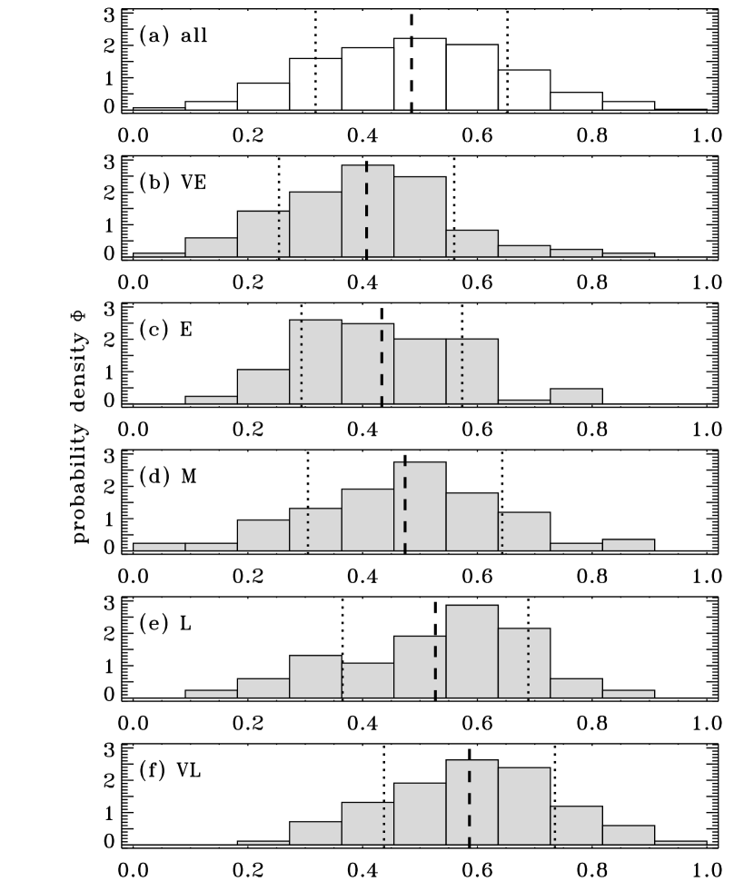
Figure 2: Observed number distributions of $v\sin i/V_{\rm crit}$ for: (a) the full Yudin (2001) database of 462 stars having nonzero $v\sin i$; (b)–(f) the five subpopulations, defined by the $T_{\rm eff}$ bounds given in in Table 1. These ratios are computed using the high-end (Cranmer) calibration for $V_{\rm crit}$. Also shown are the means (dashed lines) and $\pm$1$\sigma$ standard deviations (dotted lines) for each of the independently normalized distributions.

Figure 2 displays the number distribution of $v\sin i/V_{\rm crit}$ for all 462 Be stars, as well as the distributions for the five subpopulations defined in Table 1, each normalized to an integral of unity (i.e., expressed as binned probability densities). As noted by Yudin (2001), the mean values of $v\sin i/V_{\rm crit}$ have a systematic dependence on $T_{\rm eff}$, increasing monotonically from $\sim$0.4 for the hottest (VE) stars to $\sim$0.6 for the coolest (VL) stars. There is no clear spectral type dependence on the standard deviations (or higher moments) of the subpopulation distributions. The distributions are plotted by dividing the region between $v\sin i/V_{\rm crit}=0$ and 1 into 11 equally spaced bins; this provides a good balance between resolution and statistics. Note that the smallest and largest computed values of $v\sin i/V_{\rm crit}$ for the full database are 0.035 and 0.912. (The fact that there are no stars with measured $v\sin i$ that exceed $V_{\rm crit}$ tends to support the conclusion reached below that Be stars are not all rotating critically; see also § 4).

As an alternate derivation of the normalized projected rotation speeds, the 462 $v\sin i$ values were also divided by the lower $V_{\rm crit}$ values indicated by Chauville et al.  (2001). A least-squares power-law fit was found for the spectral type dependence of the critical rotation speeds from that paper: $V_{\rm crit}=(450\,\,\mbox{km}\,\,\mbox{s}^{-1})/s^{0.775}$, where $s$ is a continuous variable that straightforwardly denotes the spectral subtype (for O5, B0, and B9, $s=0.5$, 1.0, and 1.9, respectively). This fit does not reflect the spread in values from the range of luminosity classes (see Figure 1) but it accurately models the trend for the Chauville et al.  critical speeds to be lower than those derived by others. Table 1 gives the mean, standard deviation, skewness, and kurtosis of the $v\sin i/V_{\rm crit}$ distributions for each subpopulation using this alternate calibration for $V_{\rm crit}$. For the earliest spectral bin, VE, the mean ratio of 0.49 is only slightly higher than the value of 0.41 that corresponds to the $V_{\rm crit}$ calibration derived above. The differences between the two calibrations grow steadily larger for the cooler spectral bins, leading to mean ratios of either 0.90 (Chauville et al.) or 0.59 (Cranmer) for the VL subpopulation, depending on $V_{\rm crit}$. For the entire database, the mean ratio using the Chauville et al.  calibration for $V_{\rm crit}$ is 0.627; this is very close to the value of 0.65 given by Chauville et al.  (2001) for their sample of 116 Be stars. This value is almost 30% higher than the mean ratio of 0.485 that was computed above, and the difference is due solely to the differences in stellar mass and radius that go into the calculation of the critical rotation speed.

3 Forward Modeling of Distributions of the Projected Rotation Speed

In this section the procedure for simulating theoretical distributions of $v\sin i/V_{\rm crit}$ for a random sample of Be stars is described. The simulation of $v\sin i$ measurements for individual gravity darkened stars is outlined in § 3.1 (see also Collins 1974; Collins & Truax 1995; Townsend et al.  2004). The construction of theoretical probability distributions for a large number of stars, together with the comparison with the observed distributions, is described in § 3.2.

3.1 Modeling Individual Stars

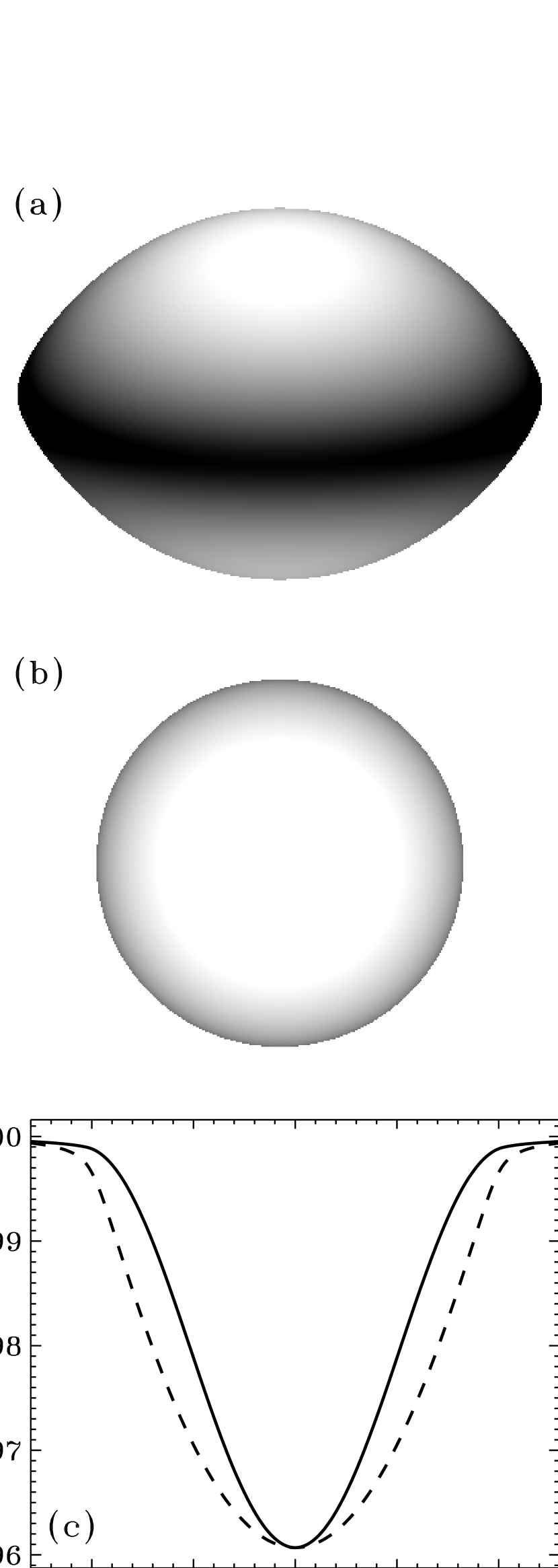
Figure 3: Schematic continuum intensity images of a B9 V star rotating rigidly with $V_{\rm eq}=0.95\,V_{\rm crit}$ and viewed from an inclination angle $i=75\arcdeg$ measured from the pole. Both images are derived with the same linear limb darkening, but they differ in that (a) uses the centrifugal force to alter the surface equipotential surfaces (Roche oblateness) and redistributes the radiative flux in proportion to the effective gravity (von Zeipel gravity darkening), and (b) does not. Panel (c) shows resulting absorption lines computed as described in the text: the solid curve corresponds to image (a); the dashed curve corresponds to (b). The central depth of profile (b) was renormalized to match that of (a) to more clearly compare the line shapes.

For a given set of fundamental stellar parameters (mass, luminosity, and polar radius), an equatorial rotation rate ($V_{\rm eq}$), and an observational inclination angle ($i$), it is possible to compute unique absorption line profile shapes that can be used as direct measures of the quantity $v\sin i/V_{\rm crit}$. Figure 3 illustrates the effect of oblateness and von Zeipel (1924) gravity darkening on the absorption line shape for a representative late-B main sequence star (see also Cohen et al.  2005). As expected, gravity darkening preferentially weights the more slowly rotating polar regions and thus produces a narrower line profile than that computed without gravity darkening. To produce the images and profiles in Figure 3, the computer code from Cranmer & Owocki (1995) was used to generate high-resolution models of both a spherical star and an oblate Roche-model star with the same polar radius and equatorial rotation velocity. The stars are observed from a large distance (1000 $R_{p}$) at a given inclination angle, and the same limb darkening law is applied in both cases (see below). Each pixel of the image has a projected linear dimension of 0.008 $R_{p}$ in the plane perpendicular to the line of sight that crosses through the center of the star.

The rotationally broadened profiles, here assumed to be the commonly used He I $\lambda$4471 absorption lines, were simulated for the two cases shown in Figure 3 by the following procedure. The residual flux is defined as the ratio of the flux in the spectral line to that of the surrounding continuum,

$${\cal R}_{\nu}\,=\,\frac{\int dx\,dy\,I_{\nu,{\rm L}}(x,y)}{\int dx\,dy\,I_{\nu,{\rm C}}(x,y)}\,\,,$$ (6)

where $x$ and $y$ are spatial coordinates that specify a grid of rays parallel to the observer’s line of sight. For the subset of these rays that intercept the stellar surface, Cranmer & Owocki (1995) and Cranmer (1996) described how to convert these coordinates into star-centered spherical coordinates $r$ and $\theta$ (ignoring the azimuthal longitude $\phi$ because the stars are assumed to be axially symmetric). The colatitude $\theta$ determines the local magnitude of the centrifugally modified effective gravity, and also—for the oblate gravity-darkened case—the local effective temperature.

For simplicity, the specific intensity of the continuum is modeled as the product of a Planck function at the local effective temperature and a linear limb darkening function, i.e.,

$$I_{\nu,{\rm C}}\,=\,\frac{5}{4\pi}B_{\nu}(T_{\rm eff})\,(1-u_{c}+u_{c}\mu)\,\,,$$ (7)

where $u_{c}$ is the continuum limb darkening constant and $\mu$ is the cosine of the angle between the line of sight and the normal to the stellar surface. Below, we adopt $u_{c}=0.4$ from both a classical treatment of limb darkening for a gray temperature distribution at a continuum wavelength of 4471 Å (see eq. 10-20 of Mihalas 1978) and a numerical study of limb darkening for rapidly rotating B stars (Table 4 of Collins & Truax 1995). The specific intensity in the spectral line $I_{\nu,{\rm L}}$ is modeled as the product of $I_{\nu,{\rm C}}$ and a residual intensity $f_{\nu}$ that is computed from Milne-Eddington theory for a pure absorption line, with

$$f_{\nu}\,=\,\frac{1-u_{c}+u_{c}\mu/(1+\eta_{\nu})}{1-u_{c}+u_{c}\mu}$$ (8)

(Mihalas 1978; Collins 1989). The dimensionless line absorption coefficient $\eta_{\nu}$ is modeled as a Voigt profile that is thermally broadened and Doppler shifted by the stellar rotation,

$$\eta_{\nu}\,=\,\eta_{0}\,H(a,\xi)\,\,,$$ (9)

and

$$\xi\,=\,\frac{\nu-\nu_{0}(1+V_{\rm LOS}/c)}{V_{\rm th}\nu_{0}/c}$$ (10)

where $H(a,\xi)$ is the standard Voigt function, $\nu_{0}$ is the rest-frame frequency of the line transition, $V_{\rm LOS}$ is the projected component of the rotation velocity along the line of sight for this ray, and $V_{\rm th}$ is the thermal speed of helium atoms corresponding to the local effective temperature. The dimensionless strength of the Voigt wings is assumed here to be given by a constant value of $a=0.08$ based on standard Stark broadening for the He I $\lambda$4471 line at a mean B-star temperature of $2\times 10^{4}$ K (e.g., Griem et al.  1962; Barnard et al.  1969; Leckrone 1971).

The strength of the absorption line for each ray that intercepts the stellar surface is parameterized by the dimensionless line-center absorption coefficient $\eta_{0}$. This quantity is determined empirically from a grid of detailed spectral synthesis calculations of the He I $\lambda$4471 equivalent width from a collection of early-type atmosphere models (González Delgado & Leitherer 1999). The effective gravity and temperature at the stellar surface for each ray is used to interpolate the local equivalent width from Table 6 of González Delgado & Leitherer (1999). The conversion between $\eta_{0}$ and equivalent width $W$ is given by the theoretical curve of growth,

$$W\,=\,\frac{2u_{c}\nu_{0}V_{\rm th}}{c[(1-u_{c})\sqrt{3}+u_{c}]}\int_{0}^{\infty}d\xi\,\left[\frac{\eta_{0}H(a,\xi)}{1+\eta_{0}H(a,\xi)}\right]$$ (11)

where $W$ above is in frequency units (Mihalas 1978). This relation has been computed numerically and tabulated for the adopted values of $a$ and $u_{c}$. For B stars, the equivalent widths for individual rays span the range between 0.1 and 1.5 Å, corresponding roughly to $\eta_{0}$ values between 30 and 3000.

The procedure outlined in equations (6)–(11) is certainly more simplistic and approximate than performing full model atmosphere calculations of the relevant line profiles (as was done by, e.g., Townsend et al.  2004). However, the relative ease of computing reasonably accurate profile shapes by the above method allows very fine grids of wavelengths, inclination angles, and rotation speeds to be computed without prohibitive computational expense. These grids make possible the detailed statistical studies described below.

Spectral lines were computed for representative main sequence stars of spectral types B0, B2, B3, B5, and B9; i.e., for stars roughly at the centers of the five subpopulation bins defined in § 2. For each spectral type, line profiles for the spherical and the oblate gravity darkened cases were computed on a fine grid of 200 wavelength points, and for 100 inclinations ($i$ between 0° and 90°) and 100 equatorial rotation speeds ($V_{\rm eq}/V_{\rm crit}$ between 0 and 1). A single measure of the line width was determined from the full width at half maximum (FWHM) of the numerically computed profiles. The key parameter to be used below is the dimensionless ratio $D$, which is defined as the FWHM line width for a model star computed with oblateness and gravity darkening divided by the corresponding FWHM for the spherical model. Thus, $D$ provides an indication of the relative change in the absorption line width that is produced by the effect of gravity darkening. Figure 4 shows $D$ as a function of both $V_{\rm eq}/V_{\rm crit}$ and $i$ for the earliest and latest (B0 and B9) spectral types. The information contained in Figure 4 is essentially equivalent to that shown in, e.g., Figure 4 of Stoeckley (1968), Figure 6 of Collins & Truax (1995), Figure 1 of Townsend et al.  (2004), and Figure 7 of Frémat et al.  (2005), but for different spectral types. These other figures have tended to plot the computed line widths as functions of projected rotation speeds, which highlights the ambiguity involved with attempting to determine the product $V_{\rm eq}\sin i$ from from an “observed” $v\sin i$. The forward modeling procedure outlined in this paper is essentially free of such ambiguity.

The overall impact of the line narrowing due to gravity darkening can be understood better by converting from $D$ to the similarly defined “velocity deficiency” quantity of Townsend et al.  (2004),

$$\delta V\,=\,(1-D)V_{\rm eq}\sin i/V_{\rm crit}\,\,,$$ (12)

specifically for their fiducial case of edge-on inclination ($i={90\arcdeg}$) and $V_{\rm eq}/V_{\rm crit}=0.95$. For the five spectral subtypes, there is a gradual increase of the effect as one goes from B0 ($\delta V=12.5$%) to B9 ($\delta V=26.0$%), with intermediate values of 16.0%, 17.5%, and 21.0% for B2, B3, and B5, respectively. These values compare favorably with those given in Table 2 of Townsend et al.  (2004), which helps to validate the use of the simpler line synthesis technique described above.

There are noticeable differences between the shapes of the contours in the B0 and B9 cases shown in Figure 4. The intermediate (B2, B3, B5) spectral types have contours in $D$ that change in shape gradually between the two plotted extreme cases. These differences arise because the He I $\lambda$4471 equivalent widths, as interpolated from the modeled spectra of González Delgado & Leitherer (1999), depend on latitude differently for different ranges of effective gravity and temperature. An early (B0) model rotating at 99% of critical exhibits a maximum in $W$ at mid-latitudes of about 0.9 Å, and minima at the poles and equator of $\sim$0.75 and $\sim$0.3 Å, respectively. A similar late-type (B9) model exhibits a simpler monotonic decrease in $W$ from pole ($\sim$0.35 Å) to equator ($\sim$0.1 Å). These differences result in different spectral line shapes and different intensity weightings over the oblate surfaces.

The procedure to simulate a measurement of $v\sin i/V_{\rm crit}$ for an individual star is summarized by the following relation:

$$\left(\frac{v\sin i}{V_{\rm crit}}\right)_{\rm\!meas}\,=\,\left(\frac{V_{\rm eq}}{V_{\rm crit}}\right)D\sin i\,(1+\zeta)\,\,.$$ (13)

The choice of a range of values for $V_{\rm eq}/V_{\rm crit}$ is discussed below in § 3.2, and the inclination angle $i$ is defined formally as $\cos^{-1}\mu_{i}$, where $\mu_{i}$ is chosen randomly from a uniform probability distribution between 0 and 1 (see also Chandrasekhar & Münch 1950). The gravity darkening factor $D$ is interpolated from the grids of values that were used to generate Figure 4. The factor $\zeta$ above is a simulated observational uncertainty, which is sampled from a normal random distribution having a mean of zero and a standard deviation of $\sigma_{\zeta}$ (i.e., 68% of the time, $\zeta$ falls between $-\sigma_{\zeta}$ and $+\sigma_{\zeta}$). The “mean uncertainty level” $\sigma_{\zeta}$ is kept constant for any given sample of model stars, though the effects of varying this parameter between 0 and 0.3 are explored below (see also Balona 1975). Yudin (2001) discussed the determination of standardized error bounds for the 462 observed $v\sin i$ values in the database, and found typical relative uncertainties of order 10%. Uncertainty levels up to 30% in the ratio $v\sin i/V_{\rm crit}$ may be reasonable to assume, since neither the numerator nor the denominator are known precisely.

In order to most stringently test the hypothesis that Be stars are rotating nearly critically, it would be desirable to make the assumptions that are most favorable to that hypothesis (i.e., those that tend to give largest derived values of $V_{\rm eq}/V_{\rm crit}$). Thus, if the derived rotation speeds are still substantially below critical even when those assumptions are made, the hypothesis of critical or nearly critical rotation can be ruled out at a high level of confidence. Two such assumptions regarding the use of $D$ in equation (13) are adopted here:

1. Despite the variations of $D$ as a function of spectral type, in the statistical models below we apply the grid of $D$ values computed for the B9 case to all of the spectral-type subpopulations. This is done because the B9 case shows the strongest line-narrowing effect due to gravity darkening (i.e., the lowest values of $D$ for rapid rotation and edge-on inclination). Applying this lower-limit case for $D$ in equation (13) leads to a possible overestimate of the narrowing trend and thus a systematic underestimate of $v\sin i/V_{\rm crit}$ for a specific assumed $V_{\rm eq}$. When compared with observed values of $v\sin i/V_{\rm crit}$, then, the resulting derived $V_{\rm eq}$ would end up being an overestimate.

2. The fact that $D$ is included at all in the equation above implies that the reported measurements of $v\sin i/V_{\rm crit}$ have not taken gravity darkening into account. However, several of the sources of observational $v\sin i$ data used by Yudin (2001) certainly did their best to account for gravity darkening, and thus they reported processed estimates of $V_{\rm eq}\sin i$ rather than raw measurements of $v\sin i$. If this is the case for a substantial fraction of the observations, then the use of equation (13) would lead to a systematic underestimation of $v\sin i/V_{\rm crit}$. This effect works in the same sense as the overestimation of the strength of line narrowing from using the B9 models for all spectral types.

Thus, the present models stand at one end of a continuum of modeling choices (i.e., “strong” gravity darkening effects), and the assumption of no gravity darkening (i.e., $D=1$) would stand at the opposite end. The true rotation speeds of the Be stars should fall somewhere between the values derived for these limiting cases.

3.2 Monte Carlo Distributions and Results

There have been numerous attempts to deconvolve intrinsic statistical distributions of stellar rotation speeds from the observed distributions of $v\sin i$ values. Analytic studies include Chandrasekhar & Münch (1950), Bernacca (1970, 1972), Lucy (1974), and Balona (1975). More recent efforts to determine the statistical distributions numerically—rather than just estimate mean values or assume that all stars have the same rotation rate—include Wolff et al.  (1982), Chen & Huang (1987), Porter (1996), and Brown & Verschueren (1997). Generally, these models tend to be “inverse” determinations that begin with an observed distribution function of projected rotation speeds $\Phi(v\sin i)$ and work iteratively towards a consistent form for the true distribution function of intrinsic rotation speeds $\Psi(V_{\rm eq})$. This technique becomes potentially ambiguous, though, when the line-narrowing effects of gravity darkening are taken into account; i.e., how are we to be sure that the derived solution for $\Psi(V_{\rm eq})$ is unique when an observed $v\sin i$ cannot be mapped identically to a single value of the product $V_{\rm eq}\sin i$?

Although the present forward-modeling method does not produce completely unique solutions, it treats all possible distributions on the same footing and thus is not in danger of missing potential solutions. After choosing a parameterized functional form for the distribution of rotation speeds $\Psi(V_{\rm eq})$, the parameters are varied by producing a multidimensional grid of trial distributions having the full range of combinations of parameters. (All velocities here are assumed to be in units of $V_{\rm crit}$.) Each trial distribution is converted into an observed distribution $\Phi(v\sin i)$ by using equation (13), and each of these is compared to the observed distributions for the five spectral-type subsamples shown in Figure 2. The best fits are judged with the $\chi^{2}$ diagnostic appropriate for comparing a coarsely sampled observed distribution with a known model distribution (see below).

Earlier studies have used various functional forms for $\Psi(V_{\rm eq})$ such as Dirac delta functions, Gaussians, and uniform (i.e., flat-topped) distributions. After some experimentation, it was found that a truncated linear function of the form

$$\Psi(V_{\rm eq})\,=\,\left\{\begin{array}[]{ll}mV_{\rm eq}+b\,\,,&V_{\rm min}\leq V_{\rm eq}\leq V_{\rm max}\\ 0\,\,,&\mbox{otherwise,}\\ \end{array}\right.$$ (14)

best balanced the demands of versatility and simplicity. (From their appearance when plotted, these distributions can also be called “trapezoidal.”) The three free parameters of this family of functions are the minimum and maximum truncation values ($V_{\rm min}$ and $V_{\rm max}$) and the slope $m$. For any choice of these parameters, the constant $b$ is determined automatically by assuring that $\Psi(V_{\rm eq})$ is normalized to unity upon integration over all $V_{\rm eq}$. The minimum and maximum possible slopes are defined by the distribution being “right triangular;” i.e., the minimum slope occurs when $\Psi(V_{\rm min})$ is the global maximum and $\Psi(V_{\rm max})=0$. The maximum slope occurs when $\Psi(V_{\rm max})$ is the global maximum and $\Psi(V_{\rm min})=0$. Thus it is convenient to define a dimensionless parameter $S$ that ranges between $-$1 and $+$1, with the slope ranging from its minimum to its maximum value over this range, and

$$m\,=\,\frac{2S}{(V_{\rm max}-V_{\rm min})^{2}}\,\,,$$ (15)

$$b\,=\,\frac{1}{V_{\rm max}-V_{\rm min}}\left[1-S\left(\frac{V_{\rm max}+V_{\rm min}}{V_{\rm max}-V_{\rm min}}\right)\right]\,\,.$$ (16)

The parameter $S$ tends to give a better qualitative impression of the shape of the function than does $m$.

For each choice of the above parameters, the resulting distribution function $\Psi$ then needs to be converted into a distribution function $\Phi$ for the observed values of $v\sin i/V_{\rm crit}$. Rather than simulating large numbers of stars for each point in the three-dimensional grid of parameter space ($V_{\rm min}$, $V_{\rm max}$, $S$), a series of Monte Carlo simulations was performed for a one-dimensional grid of delta-function distributions,

$$\Psi_{j}(V_{\rm eq})\,=\,\delta(V_{\rm eq}-V_{j})\,\,,$$ (17)

with 80 equally spaced values of $V_{j}/V_{\rm crit}$ ranging between 0 and 1. These distributions then served as basis functions used to build up any desired arbitrary statistical distribution. Each Monte Carlo simulation used 10⁵ model stars with random inclinations $i$ and observational uncertainties $\zeta$ as described in § 3.1, and identical values of $V_{\rm eq}=V_{j}$. Equation (13) was used to simulate individual values of $v\sin i/V_{\rm crit}$, and these values were summed into the same 11 bins as were used in Figure 2 for comparison with observations. This process yielded a a one-dimensional grid of $\Phi_{j}(v\sin i)$ functions corresponding to the delta-function $\Psi_{j}$ grid. Finally, then, the $\Phi$ function corresponding to a given trapezoidal distribution $\Psi$ (eq. [14]) was computed by taking the linear combination

$$\Phi(v\sin i)\,\propto\,\sum_{j}\Phi_{j}(v\sin i)\,\Psi(V_{j})\,\,,$$ (18)

and renormalizing to an integral of unity. In other words, the trapezoidal distribution $\Psi$ is used as a weighting function to determine what fraction of each of the 80 $\Phi_{j}$ functions are summed together to form the complete distribution $\Phi$.

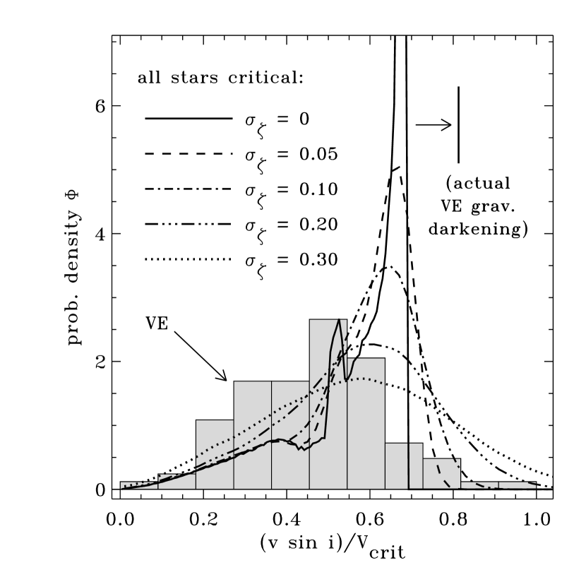
Figure 5: Statistical distributions $\Phi_{j}(v\sin i)$ computed under the assumption that all stars are rotating at $V_{\rm crit}$ and using the strongest (i.e., B9) gravity darkening grid for $D$. The simulated observations were made with varying levels of random uncertainty: $\sigma_{\zeta}=0$ (solid line), 0.05 (dashed line), 0.1 (dot-dashed line), 0.2 (dash-triple-dot line), and 0.3 (dotted line). Also plotted (gray bars) is the observed distribution of $v\sin i/V_{\rm crit}$ values for the 93 stars in the VE subpopulation, normalized using the fit to the Chauville et al.  (2001) low-end $V_{\rm crit}$ values. A vertical line in the upper-right shows how the distributions would be shifted to higher values of $v\sin i$ if the consistent gravity darkening grid for the VE stars (i.e., B0) would have been used.

Before presenting the results of the above process, it is instructive to show the $\Phi_{j}(v\sin i)$ distributions that correspond to $V_{j}=V_{\rm crit}$. These represent the predicted distributions of projected rotation speed assuming that all Be stars rotate critically. Figure 5 shows a series of these distributions that were computed for different choices for the mean uncertainty level $\sigma_{\zeta}$. For $\sigma_{\zeta}=0$, the maximum modeled value of $v\sin i/V_{\rm crit}$ is $\sim$0.68, corresponding essentially to the maximum value of $D\sin i$ along the right edge of Figure 4b. (If gravity darkening had not been taken into account, the maximum modeled value of $v\sin i/V_{\rm crit}$ for the $\sigma_{\zeta}=0$ model would have been 1.) Note the secondary peak around $v\sin i/V_{\rm crit}\approx 0.53$; this corresponds to the small local maximum in $D$ for $i\approx{40\arcdeg}$ and $V_{\rm eq}/V_{\rm crit}=1$. Predictably, when $\sigma_{\zeta}$ is increased, the probability distributions become smeared out into increasingly Gaussian shapes.

Figure 5 also shows the observed $\Phi$ distribution of the earliest-type (VE) subpopulation of Be stars, normalized by the low choice of $V_{\rm crit}$ from the fit to the Chauville et al.  (2001) values. (The distribution is shifted to the right compared to the one shown in Figure 2b.) Thus, the observed distribution is plotted with assumptions that push the peak to high values of $v\sin i/V_{\rm crit}$ and the modeled distributions are plotted with the “strong gravity darkening” assumptions that push the peaks to low values. From the fact that there is still a 15–20% mismatch between the observed and modeled peaks, despite good-faith efforts to push them together, it seems evident that the early-type Be stars cannot be all rotating with $V_{\rm eq}=V_{\rm crit}$. If the self-consistent grid of $D$ values for the B0 spectral type (shown in Figure 4a) was used instead of the lower-valued B9 grid, the modeled curves would be shifted further to the right in Figure 5 by about 18% (see vertical line in upper-right), thus making critical rotation even more of a mismatch.

The quantitative degree of agreement between a simulated distribution $\Phi(v\sin i)$ (which is known accurately) and a coarsely sampled observed distribution is determined by using the $\chi^{2}$ diagnostic defined in § 14.3 of Press et al.  (1992):

$$\chi^{2}\,\equiv\,\sum_{i=1}^{N_{b}}\frac{(n_{\rm obs}-n_{\rm mod})^{2}}{n_{\rm mod}}$$ (19)

where $N_{b}=11$ bins, and where $n_{\rm obs}$ and $n_{\rm mod}$ are the observed and modeled number counts in each bin, respectively. For the purposes of computing $\chi^{2}$, the normalized distributions are multiplied by constant factors of either 92 or 93 in order for them to contain the same total number of stars as the observed subsample distributions. For the various models discussed below, Table 1 presents normalized ratios $\chi^{2}/\nu$, where $\nu=N_{b}-1$ is the effective number of degrees of freedom. Each resulting value of $\chi^{2}$ is related to the probability that the observed counts are drawn from the same “known” distribution from which the modeled counts are drawn. Assuming normally distributed uncertainties, this probability is given by

$$Q(\chi^{2}|\nu)=\frac{1}{\Gamma(\nu/2)}\int_{\chi^{2}/2}^{\infty}e^{-t}t^{(\nu/2)-1}dt$$ (20)

where $\Gamma(x)$ is the complete Gamma function. Naturally, when $\chi^{2}\ll\nu$ the above probability approaches unity (i.e., the modeled distribution is a good match to the observations), and when $\chi^{2}\gg\nu$ the above probability is negligibly small.

To locate the optimum range of $V_{\rm eq}$ values for each subsample, the three free parameters of the trapezoidal probability distribution $\Psi(V_{\rm eq})$ were varied until global minima in $\chi^{2}/\nu$ were found. This process was repeated 7 times, once for each of the following assumed values of the mean uncertainty level: $\sigma_{\zeta}=0$, 0.05, 0.10, 0.15, 0.20, 0.25, and 0.30. In each case, the global minima in $\chi^{2}/\nu$ were located by: (1) automatically searching through the full three-dimensional parameter space, and (2) making contour plots of $\chi^{2}/\nu$ in several two-dimensional slices through the parameter space to make sure that no minima were missed. Table 1 lists the best-fit parameters and optimal values of $\chi^{2}/\nu$, $Q(\chi^{2}|\nu)$, and $\sigma_{\zeta}$ for the two assumptions concerning $V_{\rm crit}$ discussed in § 2 (i.e., high-end and low-end limits). In all cases the best fits were found with either $\sigma_{\zeta}=0.15$ or 0.20. Lower values of $\sigma_{\zeta}$ tended to produce unrealistically sharp number distributions $\Phi(v\sin i)$, and higher values produced distributions that were too broad. This seems to be an independent verification that the observational uncertainties of the Yudin (2001) $v\sin i$ values are about 10–20%.

As seen in Table 1, there were two cases where no acceptable fits could be found to the observed number distributions: the L and VL subpopulations normalized by the low-end Chauville et al.  (2001) critical rotation speeds. For these cases the peaks in the observed $\Phi(v\sin i)$ distributions occurred at values of $v\sin i/V_{\rm crit}$ larger than than 0.8, but the modeled statistical distributions—even for critical rotation—have peak values of $v\sin i/V_{\rm crit}$ no greater than $\sim$0.7, as seen in Figure 5. If the Chauville et al.  values of $V_{\rm crit}$ are correct, these late-type Be stars seem to be consistent with nearly critical rotation as well as possibly a weaker line-narrowing effect due to gravity darkening than has been modeled here.

For ease of comparison with other analyses, Table 1 also gives the weighted mean ratios of equatorial rotation speed to critical rotation speed for each subpopulation, defined by

$$\langle V_{\rm eq}/V_{\rm crit}\rangle\,\equiv\,\left[\int dx\,\Psi(x)\,x\right]\left/\left[\int dx\,\Psi(x)\right]\right.\,\,,$$ (21)

where $x=V_{\rm eq}/V_{\rm crit}$ is used for brevity. Taking into account that the five subpopulations have roughly equal numbers of stars, the mean ratio for the entire database of 462 stars is computed simply by averaging together the five values for each subpopulation. For the high-end (Cranmer) and low-end (Chauville et al.) choices of $V_{\rm crit}$ values, the weighted mean values of $\langle V_{\rm eq}/V_{\rm crit}\rangle$ are 0.684 and 0.854, respectively. The L and VL subpopulations that had no acceptable fits for $\Psi(V_{\rm eq})$ in the low-end $V_{\rm crit}$ case were assumed to be completely critically rotating, so the above weighted mean value of 0.854 is an upper limit. Frémat et al.  (2005) derived a most probable ratio of $V_{\rm eq}/V_{\rm crit}\approx 0.75$ from an analysis of the 116 Be stars published by Chauville et al.  (2001) plus 14 others. This value falls nearly halfway between the two mean ratios given above that were derived under the assumptions of lower and upper limiting cases for $V_{\rm crit}$.

Figure 6 presents a summary of the best-fit probability distributions $\Psi(V_{\rm eq})$ for each spectral-type subsample and for both the high-end and low-end calibrations of $V_{\rm crit}$. Figure 6 also compares the simulated and observed distributions of projected rotation speed $\Phi(v\sin i)$. Several features of these plots are noteworthy:

1. There is a definite dependence of $V_{\rm min}$ on spectral type. The hottest Be stars (subsamples VE and E) seem to have lower bounds on their rotation speed distributions that extend down to 40–50% of critical. This lower bound increases, as $T_{\rm eff}$ decreases, to the point where the L and VL subsamples are consistent with nearly critical rotation. An extremely approximate fit to the dependence of $V_{\rm min}$ on the stellar effective temperature is given by

   $$V_{\rm min}/V_{\rm crit}\,\approx\,0.28\,\tanh\left[13.3-(T_{\rm eff}/1500\,\mbox{K})\right]+0.72$$ (22)

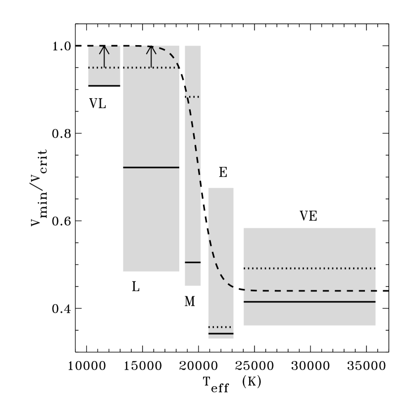
Figure 8: Minimum allowed equatorial rotation speeds for the observed populations of Be stars, plotted as dimensionless ratios $V_{\rm min}/V_{\rm crit}$ versus $T_{\rm eff}$. The empirical limits determined from $\chi^{2}$ minimization (see Table 1) are plotted as horizontal bars corresponding to the high-end Cranmer $V_{\rm crit}$ calibration (solid lines) and the low-end Chauville et al.  $V_{\rm crit}$ calibration (dotted lines). The gray bars show the range of $V_{\rm min}$ values that occur when $\sigma_{\zeta}$ is varied between 0 and 0.30 in steps of 0.05, and only high-probability values with $Q(\chi^{2}|\nu)>10$% are kept. Also shown is the approximate fitting formula given by equation 22 (dashed line).

   (see also Figure 8 below).

2. The derived values of $V_{\rm max}$ do not vary systematically with spectral type. Indeed, a decent broad-brush approximation would be to assume that $V_{\rm max}\approx V_{\rm crit}$, and that the rotation speeds of Be stars of a given spectral type range from a $T_{\rm eff}$-dependent minimum value up to the critical rotation speed.

3. The derived shapes of $\Psi(V_{\rm eq})$ depend rather strongly on the adopted mean uncertainty level $\sigma_{\zeta}$. The higher the value of $\sigma_{\zeta}$, the narrower the resulting best-fit probability distribution. This is understandable because the simulated distributions $\Phi(v\sin i)$ are modeled essentially as a convolution between two distributions: the intrinsic distribution of $V_{\rm eq}$ values and the normally distributed spread of uncertainties ($1+\zeta$). If all of these distributions were Gaussian in shape, a specified width of $\Phi$ could be obtained for an infinite number of choices for $\Psi$ and $\zeta$, as long as the root-mean-squared sum of their widths equaled the desired width of $\Phi$. Any future attempts to simulate these kinds of number distributions must be sure to model the observational uncertainties as accurately as possible.

It is also worth noting that the choice of trapezoidal parameterization for $\Psi(V_{\rm eq})$ (eq. [14]) was somewhat limiting because even the “best fitting” choices of the parameters did not yield perfect fits to the observed distributions $\Phi(v\sin i)$. For example, the strongly nonmonotonic behavior in the observed E subsample, for $v\sin i/V_{\rm crit}\approx 0.6$–0.7, limited the best-fit values of the probability $Q(\chi^{2}|\nu)$ to be never larger than 50%. A more complicated functional form for $\Psi(V_{\rm eq})$ may have been able to fit this feature better, but the introduction of too many free parameters can lead to unphysically complex distributions. An attempt was made to vary the shape of $\Psi(V_{\rm eq})$ iteratively by using a “simulated annealing” algorithm—i.e., adopting randomized changes only if they resulted in lower values of $\chi^{2}$—following the spirit, if not the exact method, of Lucy (1974). The resulting best-fit distributions always tended toward sums of several (at least 3) sharply peaked subdistributions, with large ranges of intervening $V_{\rm eq}$ having zero contribution. These distributions were judged to be unphysical, and the more smoothly varying trapezoidal distribution was determined to be the best balance of realism and parameter flexibility.

To develop a complete understanding of what ranges of $V_{\rm eq}$ can actually be ruled out by this analysis, it is not enough to plot only the best-fit distributions. Figure 7 provides a summary of the goodness-of-fit probabilities $Q(\chi^{2}|\nu)$ that were obtained both from the unconstrained parameter variation and also from other constrained searches of parameter space that examined only stars rotating faster than certain threshold values of $V_{\rm eq}$. Only results for the VE and M spectral subranges are shown, since the intermediate E subrange exhibits similar probability curves as the VE case and the L and VL cases are consistent with nearly critical rotation (and thus show no interesting behavior as the threshold lower limits are varied). These curves show how the probabilities for each subsample decrease when successively higher (i.e., more limited) ranges of $V_{\rm min}$ and $V_{\rm max}$ are allowed. The probabilities given in Table 1 for unconstrained searches of parameter space are shown in Figure 7 as the maximum values at the left edges of each plot. It is clear from Figure 7a that the VE number distribution $\Phi(v\sin i)$ cannot be fit adequately with values of $V_{\rm eq}$ that all exceed $\sim$0.8—no matter the choice of $V_{\rm crit}$ calibration. On the other hand, the necessity of subcritical rotation speeds for the M number distribution (in Figure 7b) depends sensitively on the adopted $V_{\rm crit}$ calibration. For the high-end (Cranmer) values, no good fits can be obtained when $V_{\rm eq}$ is constrained to be greater than 0.8. For the low-end (Chauville et al.) values, though, critical rotation has just a slightly lower probability than nearly any degree of subcritical rotation and thus cannot be ruled out.

The above constraints put on $V_{\rm min}$ represent determinations of the threshold values of the equatorial rotation speed for the occurrence of the Be phenomenon. Figure 8 gives a summary of the $T_{\rm eff}$ dependence of the threshold rotation speeds from Table 1 and equation (22), as well as an indication of how $V_{\rm min}$ changes for non-optimal values of $\sigma_{\zeta}$ (see caption for selection criteria). It should be emphasized that these values were all computed by assuming a relatively strong line-narrowing effect from von Zeipel gravity darkening. This assumption of $D<1$ for fast rotation tends to transform a given distribution $\Psi(V_{\rm eq})$ into a distribution $\Phi(v\sin i)$ which is shifted more toward lower values of $v\sin i$ than would have occurred if $D=1$. If, though, $D=1$ had been assumed in the above parameter optimization, the resulting values of $V_{\rm min}$ would have all been smaller than the values given in Table 1 and Figures 6 and 8. Therefore, the values of $V_{\rm min}$ derived here seem to be conservative upper bounds on the threshold for forming Be-star disks. If the gravity darkening effects were overestimated, then the $V_{\rm min}$ values may be lower, but it is difficult to imagine how they could be substantially higher.

4 Departures from von Zeipel gravity darkening?

The statistical results described in § 3 depend somewhat sensitively on the presumed form of gravity darkening used for the rapidly rotating stars. For stars with $T_{\rm eff}\gtrsim 8000$ K it is traditional to assume that the mainly radiative energy transfer in the subsurface layers maintains the ideal von Zeipel (1924) linear scaling between emergent flux $F$ and effective gravity $g$ (i.e., $F\propto g$). Cooler stars that exhibit subsurface convection are well-known to show weaker gravity darkening, with $F\propto g^{4\beta}$ and the gravity darkening exponent $\beta\lesssim 0.1$ (see, e.g., Lucy 1967; Osaki 1970; Anderson & Shu 1977; Claret 1998, 2000, 2003). Hot stars, though, may exhibit departures from the fully radiative gravity darkening value of $\beta=0.25$ if they are differentially rotating (Smith & Worley 1974), if they are in close binary systems undergoing mass transfer (Unno et al.  1994), or if there is some kind of shear-driven turbulence in their outermost layers that might help to redistribute the flux (e.g., Smith 1970; Smith & Roxburgh 1977). Some observational evidence exists from eclipsing binary light curves that $\beta$ could be greater than 0.25 in some cases (Kitamura & Nakamura 1988; Nakamura & Kitamura 1992; Djurašević et al.  2003).

A general relationship between the bolometric flux $F$ and the effective gravity $g$ (the latter defined as the magnitude of the vector sum of gravity and the outward centrifugal force) is expressible as

$$F(\theta)=\sigma_{B}T_{\rm eff}^{4}(\theta)\,=\,\left(\frac{L_{\ast}}{\Sigma_{4\beta}}\right)g^{4\beta}\,\,,$$ (23)

where $\theta$ is the colatitude measured from the pole, $\sigma_{B}$ is the Stefan-Boltzmann constant, and $\beta$ is the exponent defined in terms of effective temperature (i.e., $T_{\rm eff}\propto g^{\beta}$). Small changes in $L_{\ast}$ as a function of the rotation rate of the star are neglected (see, however, Frémat et al.  2005). The parameter $\Sigma_{4\beta}$ is a normalizing constant that is a function of the rotation rate, but is not a function of $\theta$. It is important to perform this normalization properly, since a key part of the $v\sin i$ analysis involves the comparison of stars modeled with and without gravity darkening. (In other words, it is important to know which latitudes are brighter, and which are dimmer, when compared with a star modeled without gravity darkening.) $\Sigma_{4\beta}$ is the surface-weighted integral of $g^{4\beta}$ itself, and

$$\Sigma_{4\beta}\,\equiv\,\oint g^{4\beta}dS\,=\,2\pi\int_{0}^{\pi}\frac{g^{4\beta}R_{\ast}^{2}\sin\theta\,d\theta}{\cos\delta}\,\,,$$ (24)

where $\delta$ is the angle between the local effective gravity and the radius vector ($\cos\delta=-g_{r}/g$), and both $g$ and the stellar radius $R_{\ast}$ are functions of $\theta$ (see, e.g., Slettebak 1949; Collins 1963; Maeder 1999). The two limiting cases of $\beta=0$ (no gravity darkening) and $\beta=0.25$ (standard von Zeipel gravity darkening) give the surface area of the oblate star ($\Sigma_{0}$) and the surface-weighted effective gravity ($\Sigma_{1}$), respectively. For rigidly rotating Roche-model stars, Cranmer & Owocki (1995) presented a parameterized fit of $\Sigma_{1}$ as a function of the stellar rotation rate, and Cranmer (1996) gave a similar fit for $\Sigma_{0}$. For this paper, this function was also computed for an intermediate amount of gravity darkening between none and the standard amount ($\beta=0.125$), and also for an extreme amount ($\beta=0.4$) that was indicated by recent modeling of the light curves of early-type eclipsing binaries TT Aur and V Pup (Djurašević et al.  2003).

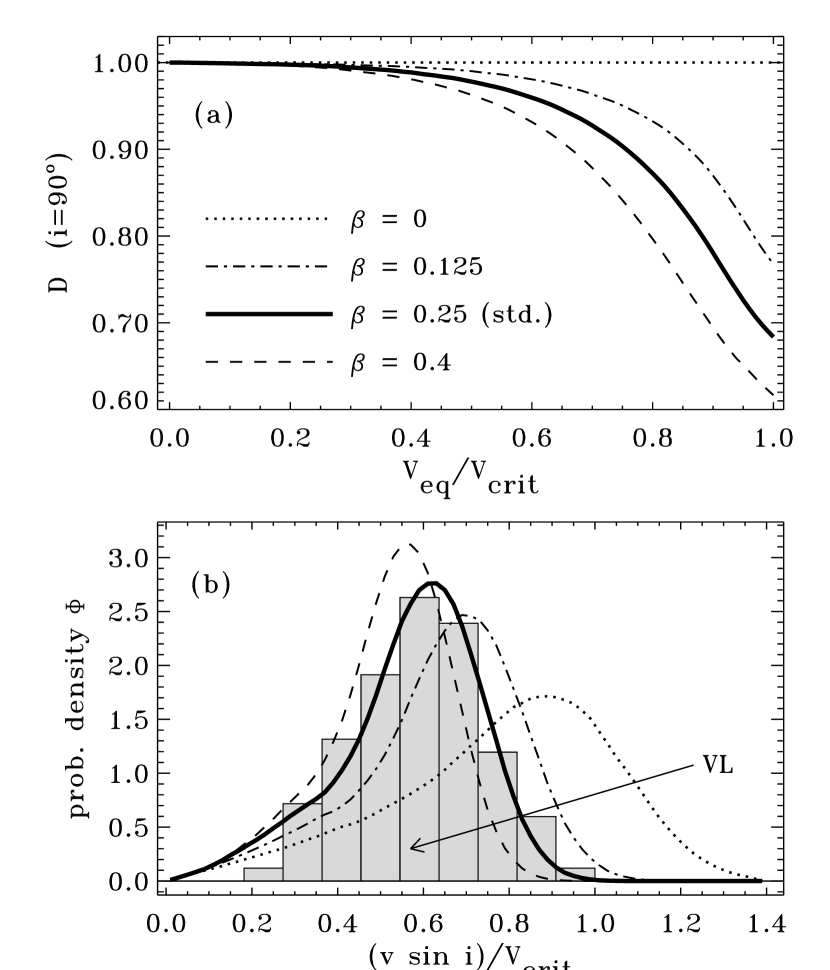
Figure 9: (a) Line narrowing ratio $D$ versus equatorial rotation speed for a constant inclination angle of 90° and a range of gravity darkening exponents $\beta$ (see labels above). (b) Statistical distributions $\Phi_{j}(v\sin i)$ computed for the same range of $\beta$ values as in panel (a), assuming that all stars are rotating at $V_{\rm crit}$ and have a mean uncertainty level $\sigma_{\zeta}=0.15$. Also plotted (gray bars) is the observed distribution of $v\sin i/V_{\rm crit}$ values for the 92 stars in the VL subpopulation normalized by the high-end Cranmer calibration for $V_{\rm crit}$ (see also Fig. 2f).

The line-narrowing factor $D$ was computed for the two new choices for $\beta$ and was compared with the values plotted in Figure 4 for the B9 spectral subtype. Figure 9a shows how the decrease in $D$ with increasing $V_{\rm eq}$ becomes stronger for larger values of $\beta$. All curves are plotted for a constant inclination angle of $i=90\arcdeg$. Figure 9b illustrates how the simulated distribution of projected rotation speeds $\Phi_{j}(v\sin i)$ shifts toward lower values for stronger gravity darkening exponents. This plot shows the distributions computed for a delta-function distribution of critical rotation speeds ($V_{j}=V_{\rm crit}$) and thus is comparable to Figure 5. The curves in Figure 9b were computed assuming a mean uncertainty level of $\sigma_{\zeta}=0.15$. Note that for the case of no gravity darkening ($\beta=0$) there would be a significant number of observations of $v\sin i$ values that exceed $V_{\rm crit}$. The fact that no such observations exist in the Yudin (2001) database implies that gravity darkening does need to be taken into account when processing the existing measurements of $v\sin i$. Figure 9b also shows the observed number distribution for the VL subsample of late-type Be stars, as normalized by the larger set of critical rotation speeds derived in § 2. The curve corresponding to $\beta=0.25$ seems to be the most consistent with the observations, although values $\pm 0.05$ would also be reasonable. The shape of the observed probability distribution—especially at its upper end—may thus be a good diagnostic of the degree of gravity darkening that is present in a population of nearly critical rotators.

5 Linear Polarization

Until this point there has not been much discussion of the dense circumstellar disks around Be stars that presumably exist only when $V_{\rm eq}>V_{\rm min}$. A primary source of information about these disks is the measurement of linear polarization produced at broadband visible wavelengths (Coyne & McLean 1982; Bjorkman 2000b) by Thomson scattering of free electrons in the flattened envelope. The Yudin (2001) database contains 335 entries with nonzero values of both $v\sin i$ and the visible polarization fraction $P_{V}$. Several aspects of the observed “triangular” distribution of $P_{V}$ versus $v\sin i$ were not easily explainable in terms of earlier models of Thomson scattering in circumstellar disks. Thus, the goal of this section is to use the stellar rotation properties derived above to produce a more accurate simulated distribution of polarization values and compare with the measured values. However, this is not an attempt to produce rigorous models of the physical properties of Be-star disks, but only a general consistency test for the validity of the derived ranges of rotation rate.

Polarization values for a simulated distribution of Be stars were computed from a slightly modified form of the single-scattering approximation formulae of McDavid (2001). The required properties for each star were found by first computing three random quantities: (1) the inclination of the rotation axis, assumed to be identical to the disk axis, using the same procedure as outlined earlier; (2) the stellar spectral type, which was specified by a nonrotating value of $T_{\rm eff}$ and was sampled from a cumulative probability distribution that was tabulated from the full Yudin (2001) database of 627 stars; and (3) the rotation rate $V_{\rm eq}/V_{\rm crit}$, which was sampled from a flat distribution ($S=0$) between $V_{\rm min}$ as given by equation (22) and $V_{\rm max}=V_{\rm crit}$. The remaining basic stellar parameters ($R_{p}$, $M_{\ast}$, and $L_{\ast}$) were interpolated from the relationships derived in § 2, assuming that all stars are on the main sequence (luminosity class V). The equatorial values of the stellar radius $R_{\rm eq}$ and effective temperature $T_{\rm eq}$ were computed assuming Roche oblateness and ideal von Zeipel gravity darkening ($\beta=0.25$). The disk temperature ($T_{\rm disk}$) was assumed to be constant and equal to 0.75 times $T_{\rm eq}$ (McDavid 2001).

The disk itself was modeled as occupying a spherical sector around the equatorial plane with an opening half-angle $\alpha$. The disk extends from its inner edge (assumed to be coincident with the star’s equatorial radius $R_{\rm eq}$) to infinity with a power-law dependence of electron density with radius,

$$N_{e}(r)\,=\,N_{e,0}\,(r/R_{\rm eq})^{-\eta}\,\,.$$ (25)

Following McDavid (2001), the constant value of $\eta=3.1$ is adopted for all stars. In an attempt to account for the large variation of fundamental parameters across the B-type spectral range, the inner disk density $N_{e,0}$ was assumed to depend on $T_{\rm eff}$ as

$$N_{e,0}\,\approx\,7\times 10^{11}\left(\frac{T_{\rm eff}}{10000\,\mbox{K}}\right)^{2.2}\,\,\mbox{cm}^{-3}\,\,.$$ (26)

This relation was derived from a linear fit (in $\log T_{\rm eff}$ versus $\log N_{e,0}$) to a total of 23 measured inner disk densities for Be stars with spectral types ranging between B0.5 and B8 (Waters et al.  1987; McDavid 2001). Figure 10 shows the $T_{\rm eff}$ dependence of these values and compares the measurements to the above fit. The estimated mass densities $\rho$ were computed under the assumption of complete hydrogen ionization; thus $\rho=N_{e}m_{\rm H}$ where $m_{\rm H}$ is the mass of a hydrogen atom.

To gauge the approximate validity of the derived inner disk densities, Figure 10 also plots two other densities that are expected to bracket these values from above and below. The photospheric mass densities are computed from the criterion that, in the stellar photosphere, the Rosseland mean optical depth should have a value of approximately one:

$$\tau_{\rm R}\,\approx\,\kappa_{\rm R}\rho H\,=\,1$$ (27)

where $H$ is the photospheric scale height (proportional to $T_{\rm eff}/g$) and $\kappa_{\rm R}$ is the Rosseland mean opacity (in cm² g^-1) interpolated from the extensive tabulation of Kurucz (1992). The resulting photospheric densities were compared with densities from detailed model atmospheres and were found to agree to within about $\pm$20% (R.  L.  Kurucz 2004, private communication). Figure 10 also shows an upper limit for the mass density at the sonic point of the equatorial outflow (i.e., the radius at which the radial flow speed equals the sound speed $c_{s}$), i.e.,

$$\rho_{\rm sonic}\,=\,\frac{\dot{M}}{4\pi c_{s}r^{2}}$$ (28)

where the mass loss rate $\dot{M}$ was computed from the stellar wind parameterization of Vink et al.  (2000). The use of these values presumes that the disk mass fluxes are of the same order of magnitude as the polar wind mass fluxes (see § 5.1 of Bjorkman 2000a). The radius $r$ is set to $R_{\rm eq}$, though it should be noted that in a slowly expanding viscous decretion disk, the sonic radius may be much larger (e.g., Okazaki 2001) and thus the sonic density may be smaller. The sound speed $c_{s}$ is assumed to be constant inside the disk,

$$c_{s}\,=\,\sqrt{\gamma kT_{\rm disk}/\mu m_{\rm H}}$$ (29)

where the adiabatic exponent $\gamma$ is 5/3, $k$ is Boltzmann’s constant, and $\mu$ is the mean molecular weight of the gas (we assume $\mu=0.6$). The fact that the inner disk density falls between the photospheric density and the sonic density indicates that the base of the disk is most likely highly subsonic (i.e., close to the stellar surface), but is also sitting several scale heights above the photosphere.

The opening half-angle $\alpha$ of the equatorial envelope was computed from the basic theory of Keplerian accretion disks, with

$$\alpha\,=\,f\tan^{-1}(c_{s}/V_{\rm Kep})$$ (30)

(see, e.g., Pringle 1981). In the above equation, $V_{\rm Kep}=(GM/r)^{1/2}$ is the Keplerian azimuthal velocity at distance $r$, here computed at a fiducial distance of $2R_{\rm eq}$. The dimensionless constant $f$ is an order-unity correction factor that is adjusted to produce an overall level of polarization similar to what is observed. The shape of the resulting distribution of $P_{V}$ versus $v\sin i$ does not depend strongly on the value chosen for $f$, as long as the same value is used for all stars in the simulated sample. In the models presented below, $f=3$, which yielded a realistic range of $\alpha$ angles between 3° and 10°. The polarization from an axisymmetric disk is proportional to $\sin\alpha\,\cos^{2}\alpha$, and for the small angles assumed here this is approximately a linearly increasing function of $\alpha$.

The above properties are the necessary inputs to the single-scattering formulae of McDavid (2001). The straightforward $\sin^{2}i$ inclination dependence of that model, though, has been replaced by a more accurate relation that takes account of stellar occultation by a thin disk (i.e., eqs. [17] and [19] of Fox & Brown 1991). The McDavid (2001) model was also simplified in two ways: (1) the relatively weak non-LTE effects for hydrogen were ignored, and (2) the polarization was computed only at the center of the $V$ filter band (5500 Å) instead of using the full bandpass function. The simulated values of $v\sin i/V_{\rm crit}$ for each star were computed by using equation (13) with $\sigma_{\zeta}=0.15$.

In Figure 11, the observed and simulated distributions of $P_{V}$ are compared with one another for statistical samples of 335 stars each. The dotted triangular limits are shown only as a rough envelope of the $v\sin i$ dependent spread of values, and are the same in both plots. Despite minor differences, the shapes of the observed and modeled distributions are similar. The rising upper envelope at low values of $v\sin i$ can be understood from the approximate $\sin^{2}i$ dependence of the polarization, since the lowest projected rotation speeds correspond to the lowest inclination angles (see also McLean & Brown 1978). The decrease in the upper envelope for the largest values of $v\sin i$, however, is not so easy to interpret. Yudin (2001) suggested three possible explanations for this decrease in $P_{V}$ spread for the fastest rotators. Two of these effects (depolarization from the oblate gravity-darkened star itself, and lower intrinsic polarization for disks around the later-type stars that also have the highest values of $V_{\rm eq}$) were not thought to be strong enough to produce the observed decreases. The third proposed effect was that the opening angle $\alpha$ may be inversely proportional to $V_{\rm eq}$. Whereas something like this may have been true for the wind-compressed disk model of Bjorkman & Cassinelli (1993), the thickness of a true viscous decretion disk seems most likely to become relatively uncoupled from the rotational properties of the central object (see eq. [30]).

The simulated distribution of $P_{V}$ values shown in Figure 11b does seem to match the observed strong decrease in spread at the largest values of $v\sin i$ in Figure 11a. This was found to occur because the models were computed using the gravity darkened equatorial temperature $T_{\rm eq}$ as the argument of equation (26). The most rapidly rotating stars with the lowest values of $T_{\rm eq}$ were thus given the lowest disk densities. A contributing factor was that these stars tended to be late-type Be stars with the lowest effective temperatures and the smallest radii. The stellar radius comes into play because the electron-scattering emissivity depends on the total number of electrons in the emitting volume (i.e., on the product $N_{e}R_{\rm eq}$). It remains to be shown whether the Be stars undergoing the most rapid rotation indeed have lower-density disks as predicted above. This seems somewhat counterintuitive, since whatever mechanisms that produce the disks are likely to grow in strength as the stellar rotation increases above the disk formation threshold (presumably at $V_{\rm min}$). However, for some combinations of stellar properties and rotation rate, the mass loss from the disk may come to dominate the angular momentum transport that feeds the disk, and lower densities may occur because of greater leakage to an equatorial wind. More work needs to be done to compare the derived disk properties of stars with similar spectral types but different rotation rates.

6 Further Evidence for Subcritical Be-star Rotation

The results obtained above imply that early-type Be stars can be rotating at significantly subcritical rates (down to roughly half of their critical rotation speed). This conclusion seems at odds with the recent statistical arguments of Townsend et al.  (2004) that suggest nearly all Be stars could be rotating nearly critically. There are several additional pieces of evidence that can be brought to bear on this disagreement, and these ideas also imply subcritical rotation for at least some Be stars.

Recent interferometric observations have put constraints on the inclination angles of some bright Be stars. Specifically, both Quirrenbach et al.  (1997) and Tycner et al.  (2004) measured an extreme axial ratio for the circumstellar envelope of $\zeta$ Tau that implies $i>{70\arcdeg}$. Using values of $v\sin i$ and $V_{\rm crit}$ from Slettebak (1982) and Porter (1996), as well as assuming $i={70\arcdeg}$ in order to produce an upper limit, Tycner et al.  (2005) estimated that $V_{\rm eq}/V_{\rm crit}$ for this star is no more than $\sim$0.52. Using the range of $V_{\rm crit}$ values computed in this paper for $\zeta$ Tau and similarly dividing $v\sin i/V_{\rm crit}$ by $\sin{70\arcdeg}$ yields a slightly wider range of ratios: 0.48 to 0.56. Assuming that gravity darkening was not taken into account in the derivation of $v\sin i$, the strongest possible correction would be to divide the above ratios by the smallest allowable value of $D$ (i.e., 0.68 for a B9 star), thus giving a range of $V_{\rm eq}/V_{\rm crit}$ for this star of 0.70–0.82. Given that the minimum value of $D$ that corresponds to a B1 type star would be higher ($\sim$0.80), the subcritical nature of this star’s rotation appears definite. Future interferometric measurements are expected to bring about similar examples of firm subcritical rotation.

In addition to rotationally broadened spectral lines, another potentially useful measure of near-critical rotation may be the large-scale shape of a star’s spectral energy distribution (i.e., rotational “color effects”). It has been known for some time (e.g., Collins 1965; Kodaira & Hoekstra 1979) that gravity darkening can lead to more pronounced color variations in the ultraviolet than in the visible, though it is unclear how tightly these variations can be calibrated to provide a direct measurement of the rotation rate or the inclination. Stalio et al.  (1987) examined far-ultraviolet flux distributions of several Be stars and was able to rule out extreme gravity darkening signatures. Stalio et al.  made the preliminary conclusion that $V_{\rm eq}/V_{\rm crit}\lesssim 0.85$ for the observed stars.

Collins & Sonneborn (1977) argued that critical rotation is unlikely for all Be stars because of the large predicted photometric shift above the main sequence. B-type stars rotating at 90% of their critical angular velocity (i.e., $V_{\rm eq}/V_{\rm crit}\approx 0.73$) showed roughly a 1 magnitude increase in $V$-band absolute magnitude, while critical rotators showed more than a 2 magnitude increase. The presence of many Be stars at only $\sim$1 magnitude above the main sequence seemed to Collins & Sonneborn (1977) to be evidence against critical rotation. Note, though, that more recent calculations of photometric shifts due to rapid rotation have predicted a substantially weaker enhancement (see Figure 3 of Townsend et al.  2004).

Mennickent et al.  (1994) studied the detailed statistics of H$\alpha$ spectral line shapes as a function of $v\sin i$. From the observed spread of the measurements, they concluded that there is “…evidence for a considerable range of the true rotation velocities of Be stars: definitely there are intrinsically slow rotators among them.”

Finally, the observed variability of Be-star circumstellar envelopes may be related to the division found in this paper between subcritical rotation (for early-type Be stars) and nearly critical rotation (for late-type Be stars). Early-type Be stars are often observed to undergo strong outburst phases with an inferred rapid evacuation and refilling of the circumstellar disk region (see, e.g., Rivinius et al.  1998, 2001). Late-type Be stars are found to be comparatively quiescent, with the transitions between Be and normal-B phases being more gradual. If the rotation rates of the early-type Be stars are far below their respective $V_{\rm crit}$ limits, they may require an impulsive mechanism of disk formation. Models of isotropic ejection from a point on the star—with some material being propelled forward into orbit and some propelled backward to fall back onto the star—may be needed to explain the disks around the hottest Be stars (Kroll & Hanuschik 1997; Owocki & Cranmer 2002). If, on the other hand, the coolest Be stars have nearly critical rotation rates, rapid outbursts as described above may not be needed for material to leak outwards into a viscous decretion disk (see also Clark et al.  2003; Owocki 2005).

7 Summary and Discussion

This paper contains a statistical analysis of the equatorial rotation rates of Be stars in Yudin’s (2001) database. A new Monte Carlo forward modeling procedure was developed to simulate number distributions of $v\sin i$ for samples of strongly gravity-darkened hot stars. The parameters of the $V_{\rm eq}$ distributions that best fit the observations were determined by a rigorous search of parameter space and a minimization of the appropriate $\chi^{2}$ statistic. Although there were some variations in the resulting parameters depending on the assumed calibration of $V_{\rm crit}$, the overall results seem robust. Early-type (O7e–B2e) Be stars were found to exhibit a spread of equatorial rotation speed between a lower limit of 0.4–0.6 $V_{\rm crit}$ and an upper limit of critical rotation. Late-type (B3e–A0e) Be stars exhibit progressively narrower ranges of rotation speed as $T_{\rm eff}$ decreases; the lower limit rises gradually to 100% of critical rotation and the upper limit remains near the critical level. Uncertainties in $V_{\rm crit}$ make it impossible to rule out critical rotation for Be stars later than about $\sim$B3, but the result of substantially subcritical rotation for B0e–B2e stars appears to be firm. This paper (see Figure 8) thus seems to imply the existence of a rough dividing line in effective temperature between two qualitatively different types of Be phenomenon:

1. For $T_{\rm eff}\gtrsim 21000\,K$ the threshold ratio $V_{\rm min}/V_{\rm crit}$ above which a disk can form is well below unity. This seems to correspond to the regime of early-type Be stars that undergo violent (possibly pulsation-driven) outbursts that feed the circumstellar disk.

2. For $T_{\rm eff}\lesssim 21000\,K$ the threshold ratio $V_{\rm min}/V_{\rm crit}$ ratio grows to unity as $T_{\rm eff}$ decreases to the end of the B spectral range. The late-type Be stars at these temperatures are seen to be more quiescent than their early-type counterparts, and this may be due to the relative ease of generating a Keplerian disk for their closer proximity to critical rotation.

The above results for early-type Be stars are in disagreement with other recent suggestions that the Be phenomenon is closely linked to critical or near-critical rotation (see, e.g., Maeder & Meynet 2000b). Pushing the $V_{\rm min}$ threshold down to significantly subcritical rotation speeds makes it more difficult to explain the existence of Keplerian decretion disks around Be stars.

The analysis presented in this paper can be improved in several ways to increase confidence in the results. The observational determination of $v\sin i$, $V_{\rm crit}$, and possibly also the inclination angle $i$ itself can be done more rigorously for an individual star when more than just one line profile is available (Stoeckley & Buscombe 1987; Reiners 2003; Frémat et al.  2005). For large $v\sin i$ databases like that of Yudin (2001), the tabulated observational uncertainties should be utilized to a greater degree in producing comparable simulated samples. The assumption used in this paper of normally distributed uncertainties normalized by a single value of $\sigma_{\zeta}$ may have contributed to systematic biases that a more observationally guided procedure could correct.

The various analyses performed here should also be done for catalogs of normal B-type stars that do not exhibit emission lines (see, e.g., Głȩbocki & Stawikowski 2000; Abt et al.  2002). It is still unclear if exceeding the minimum threshold rotation speed determined in this paper is both necessary and sufficient for the onset of the Be phenomenon; there may be many non-Be stars with $V_{\rm eq}>V_{\rm min}$. It is also not clear what sets the observed fraction of Be-star incidence as a function of the larger population of early-type stars (see, e.g., Zorec & Briot 1997; Penny et al.  2004). Firmer constraints on the rotation distributions of each population would be helpful. The definition of a truly “normal” B star is problematic, though, because a Be star can spend many years in a phase without a circumstellar disk and thus would have exhibited no Balmer emission over the entire time period of observations. There may be many early-type stars that will eventually become Be stars but are still classified as normal B stars.

Our understanding of the rotation threshold for the onset of the Be phenomenon can be aided by incorporating other kinds of observations that were not studied in this paper. Better interferometric measurements that can constrain tightly both the stellar oblateness and the circumstellar disk geometry (McAlister et al.  2005; Tycner et al.  2005) are becoming more widely available. In the long term, space-based missions like the proposed Stellar Imager may provide direct images of the oblate and gravity darkened stellar surfaces as well as firm constraints on differential rotation and macroturbulence (Carpenter et al.  2004). Measuring the widths of lines that are formed in the narrow “boundary layer” above the subcritical photosphere, but below the inner edge of the Keplerian disk (e.g., Chen et al.  1989), may be a crucial probe of the physical origin of the Be phenomenon.

Table 1: Be Star Rotational Properties by Subpopulation

	VE	E	M	L	VL
Definitions:
min $(T_{\rm eff})$ (K)	24000	20500	18500	13200	10000
max $(T_{\rm eff})$ (K)	36000	24000	20500	18500	13200
approx.  spectral types	O7–B1.5	B1.5–B2.5	B2.5–B3.5	B3.5–B6	B6–A0
number of stars	93	93	92	92	92
Observed statistics (Cranmer’s $V_{\rm crit}$):
mean $(v\sin i/V_{\rm crit})$	+0.4069	+0.4335	+0.4740	+0.5269	+0.5863
std.  dev.  $(v\sin i/V_{\rm crit})$	+0.1527	+0.1401	+0.1693	+0.1619	+0.1490
skewness $(v\sin i/V_{\rm crit})$	+0.2625	+0.3260	$-$0.1048	$-$0.4354	$-$0.1232
kurtosis $(v\sin i/V_{\rm crit})$	+0.1242	$-$0.4883	$-$0.1489	$-$0.5136	$-$0.3359
Observed statistics (Chauville et al.  $V_{\rm crit}$):
mean $(v\sin i/V_{\rm crit})$	+0.4926	+0.5225	+0.5812	+0.6795	+0.8957
std.  dev.  $(v\sin i/V_{\rm crit})$	+0.1837	+0.1661	+0.2061	+0.2144	+0.2544
skewness $(v\sin i/V_{\rm crit})$	+0.2230	+0.1964	$-$0.4215	$-$0.7592	$-$1.2430
kurtosis $(v\sin i/V_{\rm crit})$	+0.3961	$-$0.7920	$-$0.5134	$-$0.3913	$-$0.4913
Best-fit $V_{\rm eq}$ distributions (Cranmer’s $V_{\rm crit}$):
$V_{\rm min}/V_{\rm crit}$	+0.4150	+0.3423	+0.5050	+0.7219	+0.9084
$V_{\rm max}/V_{\rm crit}$	+0.7862	+0.7955	+0.9118	+0.7454	+0.9121
$S$	$-$0.9500	+0.0886	$-$0.7645	+0.6904	0
min $(\chi^{2}/\nu)$	0.39	1.31	0.58	0.44	0.57
$Q(\chi^{2}|\nu)$, in %	95.3	21.6	83.5	92.5	83.6
$\langle V_{\rm eq}/V_{\rm crit}\rangle$	+0.5416	+0.5756	+0.6562	+0.7361	+0.9103
best $\sigma_{\zeta}$	0.20	0.15	0.20	0.15	0.15
Best-fit $V_{\rm eq}$ distributions (Chauville et al.  $V_{\rm crit}$):
$V_{\rm min}/V_{\rm crit}$	+0.4914	+0.3573	+0.8832	$\gtrsim 0.95$	$\gtrsim 0.95$
$V_{\rm max}/V_{\rm crit}$	+0.9377	+0.9999	+0.8886	—	—
$S$	$-$1	+0.5882	0	—	—
min $(\chi^{2}/\nu)$	0.47	0.99	1.15	—	—
$Q(\chi^{2}|\nu)$, in %	91.4	45.1	32.0	—	—
$\langle V_{\rm eq}/V_{\rm crit}\rangle$	+0.6404	+0.7419	+0.8859	—	—
best $\sigma_{\zeta}$	0.20	0.15	0.20	—	—

Figure 1: Critical rotation speed as a function of spectral type for stars of luminosity class III (dotted line), IV (dashed line), and V (solid line). Symbols denote values of $V_{\rm crit}$ taken from other papers (see labels above).

Figure 4: Contour plots of the line narrowing ratio $D$ due to gravity darkening, for main sequence B0 (a) and B9 (b) models. The values of the constant levels are labeled above (white denotes $D\approx 1$).

Figure 6: Comparisons of observed (solid lines) and simulated (dashed lines) probability distributions of the projected rotation speed $\Phi(v\sin i)$, as well as the best-fit distributions of intrinsic rotation speed $\Psi(V_{\rm eq})$ (dotted lines) for the 5 spectral subpopulations defined in Table 1. (a)–(e): calculations assuming the high-end (Cranmer) calibration for $V_{\rm crit}$ derived in § 2. (f)–(h): calculations assuming the low-end (Chauville et al.) calibration for $V_{\rm crit}$. The L and VL models for the latter calibration did not yield acceptable solutions and are not shown.

Figure 7: Threshold goodness-of-fit probabilities $Q$ for the (a) VE and (b) M spectral subranges, computed for a range of constrained searches of parameter space. Each data point represents the maximum probability allowed when $V_{\rm min}$ and $V_{\rm max}$ were required to exceed the threshold values plotted as the abscissa. Parameter searches were performed assuming both the high-end (Cranmer) $V_{\rm crit}$ calibration (solid lines) and the low-end (Chauville et al.) $V_{\rm crit}$ calibration (dashed lines), both with $\sigma_{\zeta}$ kept constant at 0.20.

Figure 10: Mass densities (in g cm^-3) computed for main sequence nonrotating B stars at various heights, versus stellar effective temperature: optical-depth-unity photosphere (solid line), an upper limit estimate for the equatorial sonic point of disk outflow (dashed line), and the fitting formula for the inner disk density given in equation (26) (dotted line). Also shown are 8 measurements of inner disk densities from Table 2 of McDavid 2001 (triangles) and 15 measurements from Tables 3 and 5a of Waters et al.  1987 (squares).

Figure 11: Correlation between visible-band polarization $P_{V}$ and projected rotation speed $v\sin i$, shown for: (a) 335 observed stars with nonzero measurements for both values from the Yudin (2001) database, and (b) 335 simulated stars, using a modified version of the method of McDavid (2001). Rough upper bounds to the spread of $P_{V}$ values are also plotted (dotted lines).

References

- (1) Abney, W. de W. 1877, MNRAS, 37, 278
- (2) Abt, H. A. 2004, ApJ, 603, L109
- (3) Abt, H. A., Levato, H., & Grosso, M. 2002, ApJ, 573, 359
- (4) Andersen, J. 1991, A&A Rev., 3, 91
- (5) Anderson, L., & Shu, F. H. 1977, ApJ, 214, 798
- (6) Balona, L. A. 1975, MNRAS, 173, 449
- (7) Barnard, A. J., Cooper, J., & Shamey, L. J. 1969, A&A, 1, 28
- (8) Bernacca, P. L. 1970, in IAU Colloq. 4, Stellar Rotation, ed. A. Slettebak (Dordrecht: Reidel), 227
- (9) Bernacca, P. L. 1972, ApJ, 177, 161
- (10) Bjorkman, J. E. 2000a, in IAU Colloq. 175, ASP Conf. Ser. 214, The Be Phenomenon in Early-type Stars, ed. M. A. Smith, H. F. Henrichs, & J. Fabregat (San Francisco: ASP), 435
- (11) Bjorkman, J. E., & Cassinelli, J. P. 1993, ApJ, 409, 429
- (12) Bjorkman, K. S. 2000b, in IAU Colloq. 175, ASP Conf. Ser. 214, The Be Phenomenon in Early-type Stars, ed. M. A. Smith, H. F. Henrichs, & J. Fabregat (San Francisco: ASP), 384
- (13) Brown, A. G. A., & Verschueren, W. 1997, A&A, 319, 811
- (14) Carpenter, K. G., et al. 2004, Proc. SPIE, 5491, 28
- (15) Chandrasekhar, S., & Münch, G. 1950, ApJ, 111, 142
- (16) Chauville, J., Zorec, J., Ballereau, D., Morrell, N., Cidale, L., & Garcia, A. 2001, A&A, 378, 861
- (17) Chen, H.-Q., & Huang, L. 1987, Chinese Astron. Astrophys., 11, 10
- (18) Chen, H., Ringuelet, A., Sahade, J., & Kondo, Y. 1989, ApJ, 347, 1082
- (19) Claret, A. 1998, A&AS, 131, 395
- (20) Claret, A. 2000, A&A, 359, 289
- (21) Claret, A. 2003, A&A, 406, 623
- (22) Claret, A. 2004, A&A, 424, 919
- (23) Clark, J. S., & Steele, I. A. 2000, A&AS, 141, 65
- (24) Clark, J. S., Tarasov, A. E., & Panko, E. A. 2003, A&A, 403, 239
- (25) Cohen, D. H., Hanson, M. M., Townsend, R. H. D., Bjorkman, K. S., & Gagné, M. 2005, in The Nature and Evolution of Disks around Hot Stars, ed. R. Ignace & K. G. Gayley (San Francisco: ASP), in press (astro-ph/0410317)
- (26) Collins, G. W., II 1963, ApJ, 138, 1134
- (27) Collins, G. W., II 1965, ApJ, 142, 265
- (28) Collins, G. W., II 1974, ApJ, 191, 157
- (29) Collins, G. W., II 1989, The Fundamentals of Stellar Astrophysics (New York: Freeman)
- (30) Collins, G. W., II, & Sonneborn, G. H. 1977, ApJS, 34, 41
- (31) Collins, G. W., II, & Truax, R. J. 1995, ApJ, 439, 860
- (32) Collins, G. W., II, Truax, R. J., & Cranmer, S. R. 1991, ApJS, 77, 541
- (33) Coyne, G. V., & McLean, I. S. 1982, in IAU Symp. 98, Be Stars, ed. M. Jaschek & H.-G. Groth (Dordrecht: Reidel), 77
- (34) Cranmer, S. R. 1996, Ph.D. Dissertation, University of Delaware
- (35) Cranmer, S. R., & Owocki, S. P. 1995, ApJ, 440, 308
- (36) Crowther, P. A. 2005, in Astrophysics in the Far Ultraviolet, ed. G. Sonneborn, W. Moos, & B.-G. Andersson (San Francisco: ASP), in press (astro-ph/0410016)
- (37) de Jager, C., & Nieuwenhuijzen, H. 1987, A&A, 177, 217
- (38) Djurašević, G., Rovithis-Livaniou, H., Rovithis, P., Georgiades, N., Erkapić, S., & Pavlović, R. 2003, A&A, 402, 667
- (39) Doazan, V. 1982, in B Stars with and without Emission Lines, NASA SP-456, ed. A. Underhill & V. Doazan, 277
- (40) Fabregat, J., & Torrejón, J. M. 2000, A&A, 357, 451
- (41) Fitzpatrick, E. L., & Massa, D. 2005, AJ, 129, 1642
- (42) Fox, G. K., & Brown, J. C. 1991, ApJ, 375, 300
- (43) Frémat, Y., Zorec, J., Hubert, A.-M., & Floquet, M. 2005, A&A, submitted (astro-ph/0503381)
- (44) Garcia, M., & Bianchi, L. 2004, ApJ, 606, 497
- (45) Glatzel, W. 1998, A&A, 339, L5
- (46) Głȩbocki, R., & Stawikowski, A. 2000, Acta Astron., 50, 509
- (47) González Delgado, R., & Leitherer, C. 1999, ApJS, 125, 479
- (48) Gray, D. F. 1992, The Observation and Analysis of Stellar Photospheres (Cambridge: Cambridge Univ. Press)
- (49) Griem, H. R., Baranger, M., Kolb, A. C., & Oertel, G. 1962, Phys. Rev., 125, 177
- (50) Hanuschik, R. W. 1996, A&A, 308, 170
- (51) Hardorp J., & Strittmatter, P. A. 1968, ApJ, 153, 465
- (52) Harmanec, P. 1988, Bull. Astron. Inst. Czechosl., 39, 329
- (53) Harmanec, P., Bisikalo, D. V., Boyarchuk, A. A., & Kuznetsov, O. A. 2002, A&A, 396, 937
- (54) Hummel, W., & Vrancken, M. 2000, A&A, 359, 1075
- (55) Jeans, J. H. 1928, Astronomy and Cosmogony (Cambridge: Cambridge Univ. Press)
- (56) Kitamura, M, & Nakamura, Y. 1988, Ann. Tokyo Astron. Obs., 2nd Ser., 22, 31
- (57) Kodaira, K., & Hoekstra, R. 1979, A&A, 78, 292
- (58) Kroll, P., & Hanuschik, R. W. 1997, in IAU Colloq. 163, ASP Conf. Ser. 121, Accretion Phenomena and Related Outflows, ed. D. T. Wickramasinghe, G. V. Bicknell, & L. Ferrario (San Francisco: ASP), 494
- (59) Kurucz, R. L. 1992, in IAU Symp. 149, The Stellar Populations of Galaxies, ed. B. Barbuy & A. Renzini (Dordrecht: Kluwer), 225
- (60) Leckrone, D. S. 1971, A&A, 11, 387
- (61) Lucy, L. B. 1967, ZAp, 65, 89
- (62) Lucy, L. B. 1974, AJ, 79, 745
- (63) Maeder, A. 1999, A&A, 347, 185
- (64) Maeder, A., & Meynet, G. 2000a, A&A, 361, 159
- (65) Maeder, A., & Meynet, G. 2000b, ARA&A, 38, 143
- (66) Maeder, A., & Peytremann, E. 1970, A&A, 7, 120
- (67) McAlister, H. A., et al. 2005, ApJ, in press (astro-ph/0501261)
- (68) McDavid, D. 2001, ApJ, 553, 1027
- (69) McLean, I. S., & Brown, J. C. 1978, A&A, 69, 291
- (70) Mennickent, R. E., Vogt, N., Barrera, L. H., Covarrubias, R., & Ramírez, A. 1994, A&AS, 106, 427
- (71) Mihalas, D. 1978, Stellar Atmospheres, 2nd ed. (San Francisco: W. H. Freeman)
- (72) Nakamura, Y., & Kitamura, M. 1992, Ap&SS, 191, 267
- (73) Okazaki, A. T. 2001, PASJ, 53, 119
- (74) Osaki, Y. 1970, MNRAS, 148, 391
- (75) Owocki, S. P. 2005, in The Nature and Evolution of Disks around Hot Stars, ed. R. Ignace & K. G. Gayley (San Francisco: ASP), in press
- (76) Owocki, S. P., & Cranmer, S. R. 2002, in IAU Colloq. 185, ASP Conf. Ser. 259, Radial and Nonradial Pulsations as Probes of Stellar Physics, ed. C. Aerts, T. Bedding, & J. Christensen-Dalsgaard (San Francisco: ASP), 512
- (77) Penny, L. R., Sprague, A. J., Seago, G., & Gies, D. R. 2004, ApJ, 617, 1316
- (78) Porter, J. M. 1996, MNRAS, 280, L31
- (79) Porter, J. M., & Rivinius, T. 2003, PASP, 115, 1153
- (80) Press, W. H., Teukolsky, S. A., Vetterling, W. T., & Flannery, B. P. 1992, Numerical Recipes in Fortran: The Art of Scientific Computing (Cambridge: Cambridge Univ. Press)
- (81) Pringle, J. E. 1981, ARA&A, 19, 137
- (82) Prinja, R. 1989, MNRAS, 241, 721
- (83) Quirrenbach, A., Bjorkman, K. S., Bjorkman, J. E., Hummel, C. A., Buscher, D. F., Armstrong, J. T., Mozurkewich, D., Elias, N. M., II, & Babler, B. L. 1997, ApJ, 479, 477
- (84) Reiners, A. 2003, A&A, 408, 707
- (85) Rivinius, T., Baade, D., Štefl, S., Stahl, O., Wolf, B., & Kaufer, A. 1998, A&A, 333, 125
- (86) Rivinius, T., Baade, D., Štefl, S., & Maintz, M. 2001, A&A, 379, 257
- (87) Schmidt-Kaler, T. 1982, in Landolt-Börnstein: Numerical Data and Functional Relationships in Science and Technology, New Series, Vol. 2b, ed. K. Schaifers & H. H. Voigt (Berlin: Springer-Verlag)
- (88) Slettebak, A. 1949, ApJ, 110, 498
- (89) Slettebak, A. 1982, ApJS, 50, 55
- (90) Slettebak, A. 1988, PASP, 100, 770
- (91) Slettebak, A., Collins, G. W., II, & Truax, R. J. 1992, ApJS, 81, 335
- (92) Smith, B. L., & Roxburgh, I. W. 1977, A&A, 61, 747
- (93) Smith, R. C. 1970, MNRAS, 148, 275
- (94) Smith, R. C., & Worley, R. 1974, MNRAS, 167, 199
- (95) Stalio, R., Polidan, R. S., & Peters, G. J. 1987, in IAU Colloq. 92, Physics of Be Stars, ed. A. Slettebak & T. P. Snow (Cambridge: Cambridge Univ. Press), 272
- (96) Stoeckley, T. R. 1968, MNRAS, 140, 141
- (97) Stoeckley, T. R., & Buscombe, W. 1987, MNRAS, 227, 801
- (98) Struve, O. 1931, ApJ, 73, 94
- (99) Tassoul, J.-L. 1978, Theory of Rotating Stars (Princeton, NJ: Princeton Univ. Press)
- (100) Townsend, R. H. D., Owocki, S. P., & Howarth, I. D. 2004, MNRAS, 350, 189
- (101) Tycner, C., Hajian, A. R., Armstrong, J. T., Benson, J. A., Gilbreath, G. C., Hutter, D. J., Lester, J. B., Mozurkewich, D., & Pauls, T. A. 2004, AJ, 127, 1194
- (102) Tycner, C., Lester, J. B., Hajian, A. R., Armstrong, J. T., Benson, J. A., Gilbreath, G. C., Hutter, D. J., Pauls, T. A., & White, N. M. 2005, ApJ, 624, 359
- (103) Underhill, A. 1982, in B Stars with and without Emission Lines, NASA SP-456, ed. A. Underhill & V. Doazan, 3
- (104) Unno, W., Kiguchi, M., & Kitamura, M. 1994, PASJ, 46, 613
- (105) Vink, J. S., de Koter, A., Lamers, H. J. G. L. M. 2000, A&A, 362, 295
- (106) van Kerkwijk, M. H., Waters, L. B. F. M., Marlborough, J. M. 1995, A&A, 300, 259
- (107) von Zeipel, H. 1924, MNRAS, 84, 665
- (108) Walker, G. A. H., Yang, S., & Fahlman, G. G. 1979, ApJ, 233, 199
- (109) Waters, L. B. F. M., Coté, J., & Lamers, H. J. G. L. M. 1987, A&A, 185, 206
- (110) Wolff, S. C., Edwards, S., & Preston, G. W. 1982, ApJ, 252, 322
- (111) Yudin, R. V. 2001, A&A, 368, 912
- (112) Zorec, J., & Briot, D. 1997, A&A, 318, 443
- (113) Zorec, J., Frémat, Y., Ballereau, D., Chauville, J., Hubert, A.-M., Floquet, M., Levenhagen, R., & Leister, N. V. 2003, in SF2A-2003: Semaine de l’Astrophysique Française, EdP-Sciences Conf. Ser., ed. F. Combes, D. Barret, T. Contini, & L. Pagani, 617