The Physical and Photometric Properties of High-Redshift Galaxies in Cosmological Hydrodynamic Simulations

Abstract

We study the physical and photometric properties of galaxies at $z=4$ in cosmological hydrodynamic simulations of a $\Lambda$CDM universe. We focus on galaxies satisfying the “B-dropout” criteria of the Great Observatories Origins Survey (GOODS). Our goals are: (1) to study the nature of high-redshift galaxies; (2) to test the simulations against published measurements of high-redshift galaxies; (3) to find relations between photometric measurements by HST/ACS (0.4 – 1 $\mu$m) and Spitzer/IRAC (3.6 – 8 $\mu$m) and the intrinsic physical properties of GOODS “B-dropouts” such as stellar mass, stellar age, dust reddening, and star-formation rate; and (4) to assess how representative the GOODS survey is at this epoch. Our simulations predict that high-redshift galaxies show strong correlations in star formation rate versus stellar mass, and weaker correlations versus environment and age, such that GOODS galaxies are predicted to be the most massive, most rapidly star-forming galaxies at that epoch, living preferentially in dense regions. The simulated rest-frame UV luminosity function (LF) and integrated luminosity density are in broad agreement with observations at $z\sim 4$. The predicted faint end slope is intrinsically steep, but becomes shallower and is in reasonable agreement with data once GOODS selection criteria are imposed. The predicted rest-frame optical (observed $3.6\mu$) LF is similar to the rest-frame UV function, shifted roughly one magnitude (AB) brighter. We predict that GOODS detects less than 50% of the total stellar mass density formed in galaxies more massive than $\log(M_{*}/M_{\odot})>8.7$ by $z=4$, mainly because of brightness limits in the HST/ACS bands. Most of these results are somewhat sensitive to the prescription used to model the effects of dust extinction. We develop a physically-motivated model that is based on taking the simulation-predicted metallicities and using the dust-metallicity relation calibrated locally from SDSS. This model generally produces results in good agreement with observations, although it produces a modest excess of bright, rapidly star-forming galaxies. The slope of the predicted stellar mass-metallicity relation is in excellent agreement with low-redshift measurements of the stellar mass–gas-phase metallicity relation such that over two decades in stellar mass, galaxies are less enriched than low-redshift galaxies of similar stellar mass by roughly 0.6 dex. The most rapidly star forming galaxies in our simulations have rates exceeding 1000 $\mbox{M}_{\sun}\mbox{ yr}^{-1}$, similar to observed sub-mm galaxies. These galaxies are not starbursts, however, as their star formation rates show at most a mild excess ($\sim 2-3\times$) over the star formation rates that would be expected for their stellar mass. It is possible that the observable counterparts to these bright galaxies do not follow our dust prescription and are instead heavily extinguished. The overall distribution of dust reddening and mean stellar age may be constrained from color-color plots although the specific value for each galaxy cannot.

1. INTRODUCTION

According to the currently-favored hierarchical model of structure formation, the first generations of stars began forming in low-mass galaxies at very high redshift. These galaxies then grew by accreting gas from their surrounding intergalactic medium (IGM), and merged into larger galaxies that we observe today. The details of how this process operates are still not well understood. Numerical simulations that include a range of physical processes believed to govern galaxy formation allow the hierarchical scenario to be tested through detailed comparisons with observed galaxies. This yields insights into the nature of galaxy formation and assists with interpreting observations of galaxies (Weinberg et al., 2002).

The current generation of deep surveys from the optical to the radio are giving us an unprecedented view of the high-redshift ($z\gtrsim 3$) universe, and as a result are providing new and stringent tests on models of galaxy formation. Recent years have also seen a rapid growth in the power and sophistication of numerical simulations of galaxy formation, so that detailed comparisons are ever more meaningful and illustrative. For these reasons, the time is ripe for a detailed investigation into the physical nature and observable properties of high-redshift galaxies in cosmological simulations of galaxy formation.

The most effective method for finding high-redshift objects for observational study is the Lyman break selection technique (Steidel & Hamilton, 1993; Steidel et al., 1996), exploiting the large differential in flux across the rest-frame Lyman limit owing to internal absorption within the galaxy as well as strong absorption by intergalactic neutral hydrogen along the line of sight. Together with the fact that high-redshift galaxies are necessarily young and therefore blue, this endows high-redshift galaxies with distinctive colors that make photometric selection straightforward. Spectroscopic followup has shown that this technique is highly effective at isolating Lyman break galaxies (LBGs) while suffering little contamination from lower redshifts.

The first attempts to simulate LBGs used semi-analytic models (SAMs; see e.g. Kauffmann et al., 1993; Somerville et al., 2001), which employ merger trees or gravity-only numerical simulations to follow the growth of dark matter perturbations, and use analytic prescriptions to account for the remaining physical processes involved in forming galaxies such as merging, cooling, and feedback. These prescriptions give SAMs flexibility and low computational cost, but their predictions of galaxy properties consequently rely on a variety of simplifying assumptions. Hydrodynamic simulations complement the SAM approach by allowing galaxies to be simulated with minimal assumptions regarding the dynamics of gas and dark matter, but are computationally costly and are limited by numerical resolution and volume effects.

Different SAM prescriptions have yielded different physical models for LBGs, with some SAMs (notably Somerville et al., 2001) indicating that a significant fraction of LBGs are merger-induced starbursts, while others (Baugh et al., 1998) holding that LBGs are the most massive galaxies to have formed at these epochs. Hydrodynamic simulations, meanwhile, have consistently pointed towards the latter scenario (Davé et al., 1999; Nagamine et al., 2004a, 2005a; Weinberg et al., 2002). To date, efforts to infer the physical properties of LBGs via population synthesis modeling have tended to support the massive galaxy hypothesis (Shapley et al., 2005, 2001; Papovich et al., 2001; Barmby et al., 2004) although only a small subset of LBGs have had their physical properties studied in detail. In this paper, we elaborate on the predictions of the massive galaxy model in order to facilitate further comparison with current and future observational work.

While determining the basic properties of LBGs as a constraint on galaxy evolution models is an important goal unto itself, it is also a critical step towards constraining specific volume-averaged quantities such as galaxy number densities, luminosity functions (LFs), luminosity density ($\rho_{\nu}$), and the history of cosmic star formation (Madau et al., 1996; Lilly, 1997). All models of galaxy formation predict a substantial population of sources at high redshift that cannot be detected via the Lyman break technique, although they differ as to this population’s properties. For example, the SAM of Idzi et al. (2004, Figure 2) predicts a correlation between rest-frame UV flux and stellar mass that is substantially weaker than the trend from the hydrodynamic model of Davé et al. (1999, Figure 3; see also our Figure 12). Thus, the SAM used by Idzi et al. (2004) predicts that UV-faint and UV-bright galaxies are more similar in stellar mass—implying that a larger fraction of total formed stellar mass may be “missed”—than would be predicted by the hydrodynamic model of Davé et al. (1999). Testing the observable properties of LBGs against models will help in accurately assessing their contribution to global stellar mass and star formation rate budget, as well as their relationship to various other galaxy populations at those epochs.

Currently the single greatest difficulty in modeling LBGs accurately is the poorly-understood impact of extinction owing to dust. Nearly all star-forming galaxies at high redshift are seen to suffer from some level of extinction (Adelberger & Steidel, 2000; Shapley et al., 2001), usually expressed as a color excess $E(B-V)$. To date, constraints on reddening at high redshift have been obtained by fitting population synthesis models to observed LBGs (Shapley et al., 2001; Papovich et al., 2001). Unfortunately, this means the resulting distributions of $E(B-V)$ are sensitive to selection biases caused by the reddening itself, making it difficult to infer how many galaxies may be missed by such studies. In particular, as LBG selection criteria are biased against heavily reddened objects with $E(B-V)>0.3$ (Daddi et al., 2004), LBG studies are likely to underpredict the median $E(B-V)$ suffered by the complete galaxy population. In support of this, recent observations suggest that a substantial fraction of the total star formation occurring at high redshift occurs in highly reddened galaxies that are too faint in rest-frame UV to be selected as LBGs but can be selected either via their rest-frame optical colors (Daddi et al., 2004) or in the sub-millimeter (Chapman et al., 2004, 2005). The effects of dust on the most massive galaxies ($\log(M_{*}/\mbox{M}_{\sun})>11$) may not even follow simple attenuation laws such as that of Calzetti et al. (2000) (Chapman et al. 2005; Papovich et al. 2005, in preparation). Insight into the effects of dust on a galaxy’s observed spectral energy distribution (SED) and the relationship of extinction to its more fundamental properties such as stellar mass, metallicity, and star formation rate is necessary for determining the completeness of the current observational census of high-redshift galaxies. In this paper we study a range of reddening models, comparing to observations where possible, and provide an observationally-motivated reddening prescription that is the most sophisticated one used to-date in simulations.

In order to perform a meaningful statistical comparison to understand these issues, a large sample of observed LBGs is required. The Great Observatories Origins Deep Survey (GOODS) has provided an unprecedented view into the high-redshift universe (Giavalisco et al., 2004a). GOODS probes to a depth ($i_{AB}<27.5$) comparable to previous space-based observations such as the Hubble Deep Field (Williams et al., 1996) while covering an area ($320$ arcmin²) comparable to shallower ground-based studies. Combining HST/ACS data and Spitzer/IRAC data allows constraints to be placed on the star formation rate, stellar mass, extinction, and other properties of galaxies out to $z\sim 4$ and beyond (Giavalisco et al., 2004b; Papovich et al., 2004). The field size is even large enough to study clustering (Roche et al., 2003), and X-ray observations have provided auxiliary data on AGN activity and star formation (Lehmer et al., 2004). At present, 1115 LBGs at $z\sim 4$ have been isolated from GOODS data (Giavalisco et al., 2004b). Our simulations have sufficient dynamic range to numerically resolve the entire “B-dropout” sample within a comoving cosmological volume that is comparable to the volume probed by GOODS at $z\sim 4$. In addition, these simulations have been shown to broadly match the observed cosmic star formation rate density (Springel & Hernquist, 2003b; Hernquist & Springel, 2003), and the rest-frame UV luminosity functions of LBGs when a moderate amount of dust extinction is assumed (Nagamine et al., 2004a, b, 2005a; Night et al., 2005).

In this work we present comparisons between the ensemble statistical properties of high-redshift galaxies in our simulations and in the GOODS data set; examine the basic physical properties of a simulated GOODS sample and discuss the trends that emerge; investigate how the photometric properties of the GOODS sample relate to the underlying physical properties; determine how the model parameters affect the observed color-magnitude and color-color relations; discuss the extent to which the observed GOODS sample will be representative of the complete galaxy population at $z=4$; and compare our results with those of previous simulations and semi-analytic models. Our work provides a thorough investigation into using the observed photometric properties of high-redshift galaxies as a new frontier for testing galaxy formation models.

The paper is organized as follows: In Section 2 we summarize the input physics in the simulation, our procedure for identifying galaxies and computing their observed photometry, and our procedure for adding dust reddening to the simulated galaxies. In Section 3 we discuss several tests that we used to verify that our simulated galaxies’ properties are numerically resolved. In Section 4 we summarize the ensemble statistical properties of the simulated sample including incompleteness owing to the GOODS $z\sim 4$ selection function, the integrated luminosity density, and LFs. In Section 5 we present a number of plots comparing physical and photometric properties and briefly introduce the most rapidly star forming galaxies in the simulated sample. Finally, in Section 6 we present our conclusions.

2. SIMULATIONS AND SAMPLE DEFINITION

2.1. Simulations

Our work is based on cosmological hydrodynamics simulations done using GADGET-2 (Springel, 2005). GADGET-2 models the evolution of a system of particles under gravity using a Tree-particle-mesh solver and hydrodynamical forces using an entropy-conservative formulation (Springel & Hernquist, 2002) of smoothed particle hydrodynamics (SPH). Our particular simulation is the G6 simulation, an extension of the G-series runs described in Springel & Hernquist (2003b). It was started at $z=79$ with $486^{3}$ dark matter and $486^{3}$ SPH particles in a cube with periodic boundary conditions and comoving side length $100h^{-1}$ Mpc. The simulation has a SPH particle mass resolution of $9.7\times 10^{7}\;h^{-1}\;\mbox{M}_{\sun}$ and an equivalent plummer softening length of $5.33\;h^{-1}$ kpc. For comparison, we also employ the D5 simulation of Springel & Hernquist (2003b), which has higher resolution than G6, but in a smaller volume (see below). They were run using a concordant $\Lambda$CDM cosmology (Spergel et al., 2003): ($\Omega_{\mbox{m}}$, $\Omega_{\Lambda}$, $\Omega_{\mbox{b}}$, $\sigma_{8}$, $h$) = (0.3, 0.7, 0.04, 0.9, 0.7); we assume this cosmology throughout. These simulations were run on the Athlon-MP cluster at the Center for Parallel Astrophysical Computing (CPAC) at the Harvard-Smithsonian Center for Astrophysics.

Galaxy star formation histories are the key output of GADGET-2 that we use to model the observable properties of high redshift galaxies. GADGET-2 forms stars using a subgrid multiphase model for the interstellar medium (ISM; Springel & Hernquist, 2003a). If a SPH particle’s density surpasses a threshold value based on the local thermal Jeans mass, it acquires a two-phase ISM consisting of a hot ambient medium in pressure equilibrium with a cold dense medium (based on McKee & Ostriker, 1977). A thermal instability causes gas in the hot phase to cool and condense into the cold medium. The cold medium, in turn, forms stars on a timescale that is calibrated to match the observed star formation rate in local spirals (Kennicutt, 1998). A fraction of these stars forms supernovae that enrich and deposit thermal energy into the hot phase of the ISM. The thermal feedback causes cold gas to evaporate back into the ambient hot medium, depleting the gas reservoir from which stars form. In this way, GADGET-2 computes a subresolution, self-regulated star formation and feedback cycle within each star-forming SPH particle. The code also tracks the metal enrichment of each SPH particle as the simulation evolves. Star particles are spawned in two steps from each SPH particle by GADGET-2, so that each star particle has half the mass of the SPH particles. A star particle inherits the metallicity of its parent SPH particle, and does not change thereafter.

Unfortunately, by itself this multiphase ISM model cannot prevent the simulation from overproducing the observed stellar mass density in the universe, so some form of kinetic feedback is needed (Balogh et al., 2001; Kay et al., 2002; Springel & Hernquist, 2003a; Hernquist & Springel, 2003). For this reason, the simulation also includes a phenomenological Monte Carlo prescription for generating galactic superwinds as observed in local starburst galaxies. The code selects SPH particles with a star-forming ISM and gives a “kick” to their velocity vectors in the direction of the cross product of the particle’s velocity and acceleration, creating broadly bipolar outflows. The model assumes that the mass outflow rate from star forming regions is twice the local star formation rate, and the velocity of each “kick” is set to 484 km s^-1 in order to reproduce the observed space density of stellar mass at low redshift (Springel & Hernquist, 2003b). Besides suppressing star formation, this model creates qualitatively realistic large-scale galactic outflows that chemically enrich the IGM as proposed by Aguirre et al. (2001a, b), although Aguirre et al. (2005) suggest that this superwind model may require some tuning.

2.2. Galaxy Identification

We use the Spline Kernel Interpolative DENMAX (SKID) group finder to identify gravitationally bound groups of star and gas particles as galaxies. SKID operates in several steps, which may be summarized as follows: (1) slide particles along the gradient of the initial baryonic density field until they are confined into subgroups about the initial density peaks; (2) combine subgroups into groups using a friends-of-friends algorithm; (3) reject particles from each group that are not energetically bound to that group; and (4) reject groups that have fewer than a minimum number of members. We used a 16-member cutoff when running SKID but applied a much more conservative cut at 64 star particles later on (§ 3). We employ SKID rather than another group finder because test runs suggest that it separates satellite galaxies from main galaxies more accurately than halo finders that select objects based on dark matter alone. As a check we compared our results to those of Nagamine et al. (2004a), who used a different group finder with the same simulations, and found no significant differences (§ 3).

2.3. Simulated Galaxy SEDs

For each SKID-identified galaxy, we treat each star particle as a single stellar population (SSP) formed at the time the star particle was spawned. We then determine the broadband photometric properties of each galaxy by processing its star formation history through the GALAXEV library of evolutionary population synthesis models (Bruzual & Charlot, 2003), redshifting the resulting spectrum, and convolving it with our photometric filters. We use a Chabrier (2003) IMF. The filters we use here are the ACS F435W, F606W, F775W, and F850LP (hereafter, $B_{435}$, $V_{606}$, $i_{775}$, and $z_{850}$, respectively); the VLT/ISAAC $J$, $H$, and $K_{s}$; and the IRAC 3.6$\mu$, 4.5$\mu$, 5.8$\mu$, and 8.0$\mu$ ([3.6], [4.5], [5.8], and [8.0], respectively) bands. Throughout this work we use AB magnitudes (Oke & Gunn, 1983).

As the GALAXEV library covers a range of metallicities, we must decide which one to use. Figure 1 shows that simulated galaxies’ metallicities $\log(Z/\mbox{Z}_{\sun})$ at $z=4$ fall between $-0.7$ and $-0.4$. Tests showed that using the $\log(Z/\mbox{Z}_{\sun})=-0.7$ models for all galaxies produces errors of less than 0.1 magnitudes for all filters of interest, which is good enough to preserve any important qualitative trends in the data. Therefore, we present results only from models with $\log(Z/\mbox{Z}_{\sun})=-0.7$. Since much of the population synthesis work in the literature uses models with solar metallicity, we note that using the solar metallicity models would redden our galaxies by less than 0.01 magnitudes in $K_{s}$ - [3.6] ($\approx$ rest-frame $B-V$) and dim them by 0.2 and 0.3 magnitudes in rest-frame optical (observed [3.6]) and UV (observed $i_{775}$), respectively.

2.4. Reddening from Dust and the IGM

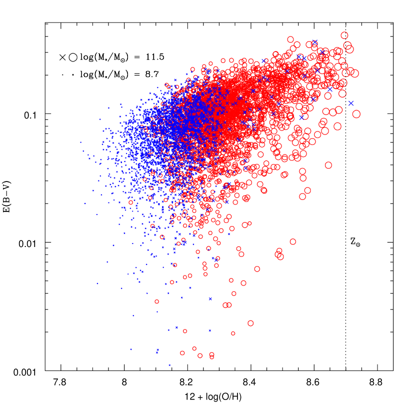
Figure 1.— The applied $E(B-V)$ distribution. The x-axis gives the metallicity of each galaxy while the y-axis gives the applied dust reddening using the Calzetti et al. (2000) reddening curve. Solar metallicity is indicated by the dotted line. Red circles and blue crosses are from the G6 and D5 simulations, respectively. Point size scales linearly with $\log(M_{*}/\mbox{M}_{\sun})$ as indicated. Note that more massive objects suffer significantly more dust reddening in this prescription.

The most common method for inferring the star formation rates of galaxies involves measuring the rest-frame UV light emitted by short-lived massive stars. Unfortunately, evidence suggests that much of the rest-frame UV light from star-forming galaxies is absorbed by a dusty interstellar medium and re-emitted at far-infrared wavelengths (Adelberger & Steidel, 2000). Both the amount of dust in each galaxy and the variation of the extinction as a function of wavelength (the “$E(B-V)$ distribution” and “reddening law,” respectively) are poorly constrained for LBGs at present. Available observational constraints tend to assume a Calzetti et al. (2000) reddening curve, which is parametrized in terms of the color excess $E(B-V)$. Several studies have derived $E(B-V)$ distributions using this law from population synthesis (Shapley et al., 2001) or UV spectral slope (Adelberger & Steidel, 2000; Ouchi et al., 2004) techniques. Consensus has centered on a median value of $E(B-V)$$\sim 0.15$ with some scatter for LBGs at $z\sim 3$, corresponding to a median factor of 3–5 extinction in the UV. For consistency with past work, we will employ the  Calzetti et al. (2000) reddening law, although we briefly consider the Charlot & Fall (2000) law as well.

Given the reddening law, a color excess $E(B-V)$ must be chosen for each galaxy. As argued above, it is not appropriate to simply apply an observed $E(B-V)$ distribution such as that of Shapley et al. (2001) to our sample, as there is no a priori reason to expect that the intrinsic and observed $E(B-V)$ distributions are the same. The intrinsic $E(B-V)$ distribution could, for example, include a significant population of highly reddened objects; the dust in such objects would render their observable rest-frame UV colors too red for them to pass the LBG color cuts that have been used to date (see e.g. the $BzK$ samples of Daddi et al., 2004).

The state-of-the-art in intrinsic $E(B-V)$ distributions is more art than science. Nagamine et al. (2004a) do not assume an intrinsic $E(B-V)$ distribution, but rather plot their results for several different uniform values of $E(B-V)$ and note that the data match the simulated LFs and number counts well if the typical $E(B-V)$ at redshifts $z\sim$ 3–5 is 0.15. By contrast, recent SAMs (Somerville et al., 2001; Idzi et al., 2004) scale reddening with UV luminosity in a way that mimics the correlations observed in nearby starburst galaxies; we will explore this $E(B-V)$ distribution, but we note that it is not well-motivated for our sample because most of our simulated LBGs are not starbursts.

Here, we employ the novel approach of inferring each galaxy’s dust content $E(B-V)$ from its metallicity. It is natural to expect a trend between reddening and metallicity since dust grains are made of metals; indeed, such a trend was first observed in IUE spectra of starbursts by Storchi-Bergmann et al. (1994). We use a correlation observed between the reddening and metallicity in the Sloan Digital Sky Survey (SDSS) main galaxy sample (C. Tremonti, private communication), extrapolating the mean trend to each galaxy’s metallicity. For each galaxy, we also add a Gaussian scatter $\delta E$ with variance equal to one half of the mean color excess $\langle E(B-V)\rangle$ at that galaxy’s metallicity; this produces a good match to scatter observed in the SDSS sample. The final relation is

$$E(B-V)=9.0\times Z^{0.9}+\delta E,$$ (1)

where $Z$ is the galaxy’s mean stellar metallicity (expressed as a ratio of the mass in metals to the total stellar mass) and the scatter $\delta E$ is of a Gaussian form given by

$$f(\delta E)\mbox{\ d}(\delta E) = \frac{1}{\frac{1}{2}\langle E(B-V)\rangle\sqrt{2\pi}}$$ (2)

$$\times \exp\left[-\frac{1}{2}\left(\frac{E(B-V)}{\frac{1}{2}\langle E(B-V)\rangle}\right)^{2}\right].$$

Figure 1 shows the results of this prescription applied to all simulated galaxies by giving the average metallicity of the star particles in each simulated galaxy versus the applied color excess $E(B-V)$. The solar abundance is marked with a dotted line. While the simulation does not trace the abundances of individual metal species, we report the metallicity as an oxygen abundance since this is a common tracer of other metals.

Figure 2.— Applied reddening $E(B-V)$ versus unextinguished flux in $i_{775}$ (rest-frame 1500 Å) for all resolved galaxies. Open triangles give our fiducial prescription and the solid line gives the mean of the prescription used in Somerville et al. (2001). Our applied reddening scales much less strongly with star formation rate than the prescription used in Somerville et al. (2001).

As we will show, this method yields results that are in broad agreement with other methods, such as applying a uniform $E(B-V)$ to all galaxies or picking $E(B-V)$ from a Gaussian distribution. It naturally produces a weak correlation between mass and reddening since galaxies with higher stellar mass tend to have higher metallicities. In principle, it also has the potential to produce massive, evolved galaxies with no gas and (unphysically) significant dust. However, inspection of our simulated B-dropout sample revealed no massive galaxies with abnormally low gas surface density or star formation rate. The lack of massive gas-free galaxies at low redshifts would certainly indicate a failing of the simulation, but it is unclear whether it is a failing at $z\sim 4$. In any case, it does remove the necessity of further refining our reddening prescription at this point.

Figure 2 shows our fiducial $E(B-V)$ distribution and compares it with the mean of the distribution used in Somerville et al. (2001) and Idzi et al. (2004). The abscissa gives the observed flux in $i_{775}$ before reddening is applied and the ordinate gives the applied reddening $E(B-V)$. To generate the curve, we adapted the Somerville et al. (2001) prescription assuming a $\lambda^{-0.7}$ reddening curve and $R_{V}=A_{V}/E(B-V)=4.05$ (Calzetti et al., 2000) to derive $E(B-V)=0.189\times 10^{0.2(24.98-i_{775})}$. Using the mean relation between the unextinguished flux in $i_{775}$ and the intrinsic star formation rate $\dot{M_{*}}$ for our galaxies that we derive as described in § 2.3, this can also be written as $E(B-V)=0.189\times 10^{(-0.44+0.52\log(\dot{M_{*}}))}$ where $\dot{M_{*}}$ is in $\mbox{M}_{\sun}\mbox{ yr}^{-1}$. While our prescription naturally leads to UV-brighter objects having greater extinction, our mean trend is not nearly as strong as theirs.

For comparison, we explore several other $E(B-V)$ distributions. In one, each galaxy’s reddening is determined randomly via a Gaussian distribution of $E(B-V)$ with mean and standard deviation 0.15 but truncated at 0.0 so that no galaxy suffers negative extinction; this is referred to hereafter as the “random” $E(B-V)$ distribution and is similar to the distribution used by Night et al. (2005). We also use a sample in which each galaxy’s reddening is set to 0.12 (the “flat” $E(B-V)$ distribution); this number was chosen to produce reasonable agreement between the simulated and observed luminosity densities in the rest-frame UV (cf. § 4.2). Unless otherwise noted, we employ our fiducial $E(B-V)$ distribution for all of our results.

Finally, in addition to dust extinction we must model attenuation owing to the IGM along the line of sight to the galaxy. We use the prescription for the mean attenuation given by Madau (1995), which accounts for a stochastic distribution of optically thin Lyman-$\alpha$ forest clouds as well as optically thick Lyman limit systems. For our $z=4$ galaxies, this prescription suppresses the simulated fluxes in the observed $B_{435}$ and $V_{606}$ bands by roughly $1.6\pm 0.1$ and $0.4\pm 0.1$ magnitudes, respectively (the scatter owes to the variation in the shapes of the intrinsic galaxy SEDS), and does not affect redder bands at all.

3. NUMERICAL RESOLUTION EFFECTS

There are a number of ways in which cosmological N-body simulations can fail to resolve the physical properties of galaxies. As a relevant example, Figure 10 in Springel & Hernquist (2003b) shows how the simulated cosmic star formation rate density at a given redshift varies with mass resolution. Broadly, using higher mass resolution allows lower-mass objects to be resolved, and allows structure formation at all scales to be resolved earlier in a simulation; by contrast, simulating a larger cosmological volume typically entails using lower mass resolution but allows rare, massive objects to be simulated. For these reasons, the cosmic star formation rate density in the G6 simulation lies below the correct value inferred from higher resolution simulations until slightly after $z=4$. During this time, some of its galaxies may possess lower stellar mass and bluer colors than the converged values. Since we are mainly considering the properties of the largest galaxies that collapsed earliest, we expect our star formation rates to show better convergence than the overall galaxy population. However, as a check that our simulated sample’s properties are resolved, we repeat our analysis with the higher-resolution D5 simulation of Springel & Hernquist (2003b), whose cosmic star formation rate density converges to the resolved value before $z=4$. D5 was started at $z=159$ with $324^{3}$ dark matter and $324^{3}$ SPH particles in a cube of comoving side length $33.75h^{-1}$Mpc. It has a SPH particle mass resolution of $1.26\times 10^{7}\;h^{-1}\mbox{M}_{\sun}$ and an equivalent Plummer softening length of of $4.17h^{-1}$kpc, and uses the same cosmology as G6.

Figure 3.— (top) The mass functions of all galaxies found by SKID in the G6 and D5 simulations. (middle and bottom) Total baryonic mass versus stellar mass for all simulated galaxies in the D5 (middle) and G6 (bottom) simulations. The discretized behavior at low stellar masses results from finite mass resolution. The heavy vertical lines indicate where our 64 star particle mass resolution cut falls in each simulation. Our stellar mass cut removes galaxies whose star formation histories are not well-resolved owing to the stochasticity in the star formation prescription.

Mass Resolution: We determined the simulated mass resolution by comparing the stellar mass functions for the G6 and D5 simulations (Figure 3, top panel). It is tempting to assume that each simulation resolves the properties of all galaxies whose stellar mass exceeds the mass at which the simulated stellar mass function tracks that of the higher resolution simulation; Figure 3 in this case tells us that the G6 resolves galaxies with stellar mass above $\log(M_{*}/\mbox{M}_{\sun})=8.5$. Unfortunately, since we are interested in star formation histories of galaxies, this criterion is insufficient. The bottom panels of Figure 3 plot the total baryonic mass versus stellar mass for the two simulations. Inspection shows that the correlation between total baryonic and stellar mass is tight at high stellar masses but becomes noisy at lower stellar masses, well before the stellar mass function turns over. This stochasticity, arising as a result of the stochastic prescription for star formation in the code, would result in unphysical scatter in our simulated star formation histories. To avoid this, we impose a stricter minimum stellar mass cut for G6 at 64 star particles or $\log(M_{*}/\mbox{M}_{\sun})=9.64$ (the solid line in the plot), which is slightly below the stellar mass observed for typical ($L^{*}$) LBGs at $z\sim 3$ (Shapley et al., 2001; Papovich et al., 2001). Above this limit, the variance in the baryonic-stellar mass relation is reasonably small, so it is mostly free of stochasticity effects. We test this more thoroughly below.

To fully probe to GOODS depth, we include results from the D5 simulation in order to fill out the low end of the mass function; using the 64 star particle criterion on D5 allows us to consider galaxies down to $\log(M_{*}/\mbox{M}_{\sun})\geq 8.76$. The normalization of the G6 mass function is lower than that of the D5 by about 40% at stellar masses below $\log(M_{*}/\mbox{M}_{\sun})=10.3$, likely the result of overmerging owing to the lower spatial resolution in G6.

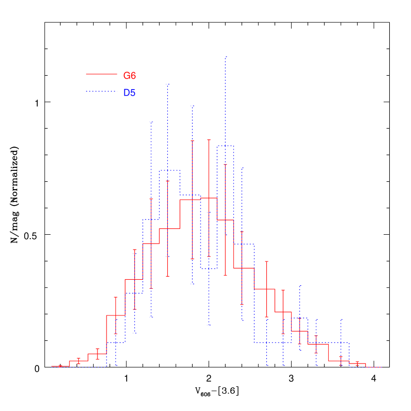
Figure 4.— Histograms of $V_{606}-[3.6]$ colors of simulated B-dropouts with optical magnitudes in the range $22<[3.6]<24.25$ from G6 (solid, red) and D5 (dotted, blue), normalized to unit area. Errors are from jackknife resampling (§ 4.2). Dust reddening has been applied via our fiducial metallicity-derived prescription. The agreement between galaxies’ colors in the high-resolution and low-resolution simulations indicates that our stellar mass cut removes galaxies whose star formation histories are not resolved in the low-resolution simulation.

Color resolution: A galaxy’s color is determined mainly by when its stars formed. In a lower resolution simulation, a galaxy remains unresolved for longer, so that its star formation is delayed. The galaxy will then be bluer than it should be, and may even experience an unphysical burst of star formation just as the density threshold for star formation is exceeded (M. Fardal, private communication). Indeed, we find that globally at $z=4$, G6 galaxies have roughly twice the birthrate (i.e. star formation per unit stellar mass) as D5 galaxies, indicating that for the general galaxy population in G6, this effect could be significant.

Does this offset in birthrates propagate into GOODS-observable quantities? One measure of the birthrate is the $V_{606}-[3.6]$ color, which probes the relative amount of light from young, OB-type stars to later-type (A and later) stars, thus constraining the ratio of the amount of recent star formation to the amount from previous events. Thus, to answer our question we constructed histograms of reddened galaxy colors in observed $V_{606}-[3.6]$ for the two simulations, shown in Figure 4. The plot shows only those galaxies whose observed IRAC 3.6$\mu$ fluxes lie in the range $22<[3.6]<24.25$ (corresponding roughly to stellar masses in the range $9.7<\log(M_{*}/\mbox{M}_{\sun})<10.5$) and which satisfy the GOODS $z=4$ LBG color and magnitude cuts (cf. § 4). There may be a slight excess at the blue end of the G6 histogram, although this may result from an underpopulated tail for the D5 distribution owing to its small volume. Overall, however, there is remarkable agreement given the different birthrates; a Kolmogorov-Smirnov test of the two color distributions yields a 99.2% probability that they are drawn from the same distribution. This suggests that the G6 simulated birthrates and colors are generally insensitive to resolution effects for our choice of a 64-star particle cut and GOODS selection.

Group Finder: The choice of group finder used to identify galaxies in the simulated data could in principle affect the overall properties of the selected sample. Typically, however, the baryonic clumps representing galaxies are much better separated than dark matter halos in such a way that unique identification is not difficult. We compared LBG number counts in the D5 and G6 simulations at $z=3$ to the results of Nagamine et al. (2004a, b), who used an entirely different group finder on the same simulations. In the G6 and D5 simulations with no reddening, they found 12,402 and 202 galaxies that consisted of at least 32 particles and satisfied the Steidel et al. (2003) color cuts, yielding comoving source densities of -1.91 and -2.28 in units log(N/$h^{-3}$Mpc³). For the same sample definition and using our group finder, we extracted 11,626 and 244 LBGs, corresponding to source densities of -1.93 and -2.19. These differences are not easy to interpret, but as they are small we proceed while bearing in mind that the choice of group finder may introduce a $\approx 10\%$ uncertainty into volume-averaged predictions; this uncertainty is small compared to, for instance, uncertainties in our reddening prescription.

4. PROPERTIES OF THE $z=4$ SAMPLE

4.1. Sample Definition

In order to lend concreteness and relevance to our simulated sample, we study those galaxies that satisfy the GOODS $z\sim 4$ LBG color selection criteria given in Giavalisco et al. (2004b):

$$(B_{435}-V_{606})\geq 1.2+1.4\times(V_{606}-z_{850})\;\wedge\;$$

$$(B_{435}-V_{606})\geq 1.2\;\wedge\;(V_{606}-z_{850})\leq 1.2.$$

Unless otherwise stated, we combine these color cuts with a magnitude cut at $z_{850}<26.5$, which is roughly the $10\sigma$ detection limit for point sources in $z_{850}$ (Giavalisco et al., 2004a). Additionally, unless otherwise stated we apply dust reddening to our sample using our fiducial metallicity-derived $E(B-V)$ distribution. In this section we discuss how these criteria confine the properties of the sample under investigation.

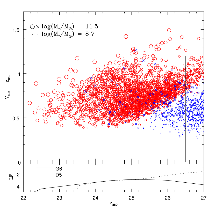
Figure 5.— (top) GOODS color-magnitude diagram of resolved G6 (red circles) and D5 (blue crosses) galaxies at z=4. Point sizes scale linearly with $\log(M_{*}/\mbox{M}_{\sun})$ as indicated. The heavy lines indicate the B-dropout color- and brightness cuts. (bottom) The $z_{850}$ LFs for the G6 (solid) and D5 (dotted) simulations in units of log(N mag^-1 $h^{3}$ Mpc^-3). The B-dropout color and magnitude cuts miss low-mass galaxies owing to faintness and massive galaxies owing to redness.

The B-dropout color cuts require that LBGs be red in $B_{435}-V_{606}$ and blue in $V_{606}-z_{850}$. Inspection revealed that all of the simulated galaxies satisfy the redness cut in $B_{435}-V_{606}$. This results directly from the Madau (1995) prescription for attenuation by the IGM, so it is not a direct prediction of our simulation. From now on, we ignore the $B_{435}-V_{606}$ color selection criterion. The upper panel of Figure 5 shows the simulated sample, before applying color and detection cuts, in the $V_{606}-z_{850}$ vs. $z_{850}$ color-magnitude space. The point sizes are scaled by stellar mass while the G6 galaxies are red and the D5 galaxies are blue. Heavy lines indicate the GOODS cuts. The magnitude cut excludes most of the low-mass galaxies and a few of the massive ones while the color cut independently excludes only a few massive galaxies. The slope of the discontinuity between the G6 and D5 samples indicates the line of constant stellar mass—at a given stellar mass, galaxies that are brighter are also bluer since both effects result from an increased star formation rate or a younger stellar population. The bottom panel plots the LF for each simulation in units of log(N mag^-1 $h^{3}$ Mpc^-3). The smooth connection between the two samples where the G6 turns over owing to our stellar mass minimum gives further evidence that the G6 galaxies are resolved down to that mass limit.

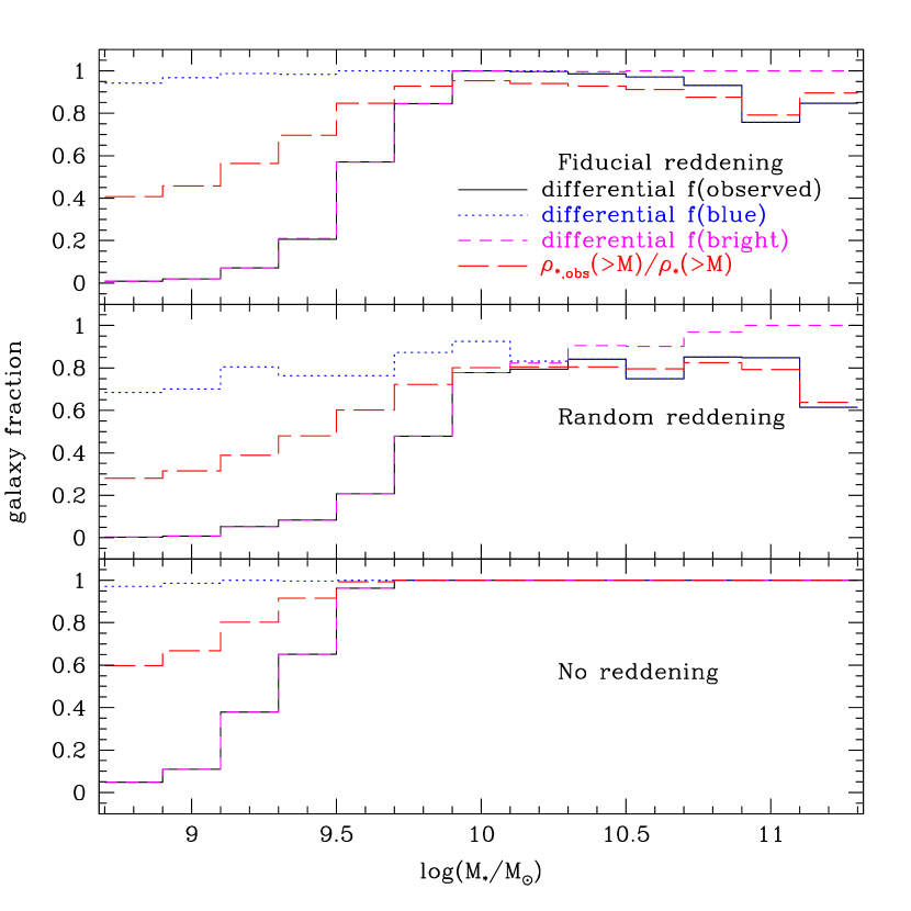
Figure 6.— The mass selection function of LBGs in the simulated GOODS sample for three different $E(B-V)$ distributions: fiducial (top), random (middle) and dust-free (bottom). In each plot the blue, dotted line gives the fraction of galaxies in that mass bin that are bluer than $V_{606}-z_{850}=1.2$; the magenta, short-dashed line gives the fraction that are brighter than $z_{850}=26.5$; the black, solid line gives the fraction that are both bright and blue; and the red, long-dashed line gives the fraction of stellar mass density in galaxies at or above that stellar mass that would be observable in GOODS. For any reasonable intrinsic $E(B-V)$ distribution, the B-dropout selection criteria remove low mass ($\log(M_{*}/\mbox{M}_{\sun})<9.5$) galaxies owing to faintness and massive galaxies owing to dust reddening.

Figure 6 shows the mass selection function of the simulated GOODS sample for the fiducial and random $E(B-V)$ distributions as well as a dust-free case (top, middle, and bottom panels, respectively); thus, the top panel is a different way of looking at Figure 5. Since none of the simulated galaxies are excluded by the cut in $B_{435}-V_{606}$, we consider only what fraction of the galaxies, as a function of stellar mass, are bluer than 1.2 in $V_{606}-z_{850}$ (dotted blue line), brighter than 26.5 in $z_{850}$ (magenta short-dashed line), or both bright and blue—that is, observable (solid black line). Not surprisingly, low-mass galaxies are missed owing to faintness while some massive galaxies are missed owing to redness. Interestingly, both of these reasonable $E(B-V)$ distributions predict that the selection functions reach their maximum around $10^{10}\;\mbox{M}_{\sun}$ with a fairly steep dropoff to lower masses. For the fiducial case, there is additionally a shallow decline toward higher masses owing to the higher reddening experienced by more massive, metal-rich galaxies. In either case, 10–20% of galaxies with stellar mass larger than $10^{10}\;\mbox{M}_{\sun}$ are missed because dust causes them to be too red in $V_{606}-z_{850}$. This effect accounts for much of the difference between reddened and unreddened rest-frame UV luminosity functions at the bright end of Figure 8.

The red long-dashed line shows, as a function of stellar mass, the cumulative fraction of stellar mass density in galaxies at or above a given stellar mass that is selected by the GOODS color and magnitude cuts and is in principle observable. This can be thought of as a normalized convolution of the mass function $\phi(m)$ with the selection function $f_{\mbox{\scriptsize obs}}(\mbox{M}_{*})$:

$${\rho_{*,\mbox{\scriptsize obs}}(>\mbox{M}_{*})\over\rho_{*}(>\mbox{M}_{*})}={\int^{\mbox{M}_{\mbox{\scriptsize max}}}_{\mbox{M}_{*}}\phi(m)f_{\mbox{\scriptsize obs}}(m)m\mbox{\ d}m\over\int^{\mbox{M}_{\mbox{\scriptsize max}}}_{\mbox{M}_{*}}\phi(m)m\mbox{\ d}m}$$ (3)

Several points are of interest. First, the simulations predict that, even in an ideal universe with no dust, no more than 60% of the total stellar mass density residing in galaxies more massive than the resolution limit at $\log(M_{*}/\mbox{M}_{\sun})=8.76$ would be observable owing largely to low-mass galaxies being too faint. In fact, this is an upper limit on the actual completeness over all galaxies since the simulated galaxy mass function is likely prolific at masses below the resolution limit. Second, once dust is added the observed fraction falls to between 30% and 40%, depending on the $E(B-V)$ distribution. Third, some fraction of real galaxies is always unobservable owing to blending with stars or other galaxies, further suppressing the fraction of stellar mass density observable; this effect is routinely accounted for via Monte Carlo simulations. Finally, it is interesting to repeat the exercise for the cumulative star formation density by simply replacing $m$ with $\dot{m}$ in the above integral, and comparing. The total cumulative fractions of stellar mass density observed are 41, 28, and 60% for the fiducial, random, and dust-free reddening distributions, respectively; the total cumulative star formation fractions observed are 51, 36, and 69% for the same distributions. Thus, the observed galaxies may contain a somewhat higher (by $\approx 10\%$) fraction of the star formation density than the stellar mass density. This is expected since the brightness cut in $z_{850}$ corresponds to a rest-frame UV selection, which is expected to trace the star formation rate better than the stellar mass. However, the small magnitude of the effect indicates that such a selection does not exclude the bulk of the stellar mass.

Previously, Nagamine et al. (2004c) compared the total density of stellar mass in the G6 simulation to observations at $z\sim 3$ and found that the simulation includes roughly twice as much stellar material as is observed at high redshift if the simulation is normalized so as to agree with observations at low redshift. They speculated that the missed stellar mass may be hidden in massive galaxies that are too red to be observed. Figure 6 continues this line of inquiry. Our findings are in qualitative agreement in that we show how no more than half of the stellar mass is likely to be observable via the Lyman break technique. We confirm that a portion of the missed stellar mass is hidden in massive, dusty galaxies, although the number of such galaxies is sensitive to the amount of dust extinction applied. However, as mentioned we also find that much—and possibly most—of the missed stellar mass at this redshift is hidden in numerous low-mass galaxies that are simply too faint to be observable rather than in massive red or “red and dead” systems.

It is interesting to compare our completeness results to those of semi-analytic models. Idzi et al. (2004) used a semi-analytic model to predict that the B-dropout selection criteria select less than 50% of the stellar mass density in galaxies more massive than $\log(M_{*}/\mbox{M}_{\sun})>9.57$. For the same range of stellar mass, we find that the B-dropout criteria select 82% and 58% of the stellar mass density for the cases of fiducial and random reddening, respectively. The difference almost certainly arises from the very different ways in which the two models treat star formation. For example, our LBGs are generally more massive than those of Idzi et al. (2004), and the trend between stellar mass and rest-frame UV flux is much stronger in our sample than in theirs (cf. their Figure 2). Our results qualitatively agree with theirs in the sense that most of the missed stellar mass results from the magnitude limit at $z_{850}<26.5$ rather than the color cuts.

The fact that a reasonable fraction of massive galaxies is missed by the $B$-dropout color cuts raises the question of whether different selection criteria could isolate a larger—or at least different—portion of the high-redshift galaxy population. Daddi et al. (2004) proposed a two-color criterion for isolating high-redshift galaxies that is intended to include highly obscured star-forming galaxies as well as massive galaxies with old stellar populations. Their criterion is $RJL\equiv(J-[3.6])-1.4(R-J)\geq 0$. This color cut excludes none of the resolved galaxies in our simulations for redshifts $z<4.7$ (by $z\approx 4.7$, the IGM substantially suppresses flux in observed $R$, rendering the galaxies too red in observed $R-J$). Hence, our simulations suggest that this may be an effective way to select galaxies that are missed by the Lyman dropout technique as long as samples are not heavily contaminated by low-redshift interlopers.

Finally, we remark on the expected sample completeness in the IRAC bands. While the rest-frame UV data probe to $z_{850}=26.5$, the IRAC data set achieves rough 5$\sigma$ detection limits of 26.1, 25.5, 23.5, and 23.4 in the [3.6], [4.5], [5.8], and [8.0] channels, respectively. Our simulations indicate that with these limits, the fraction of B-dropouts that will be detected is 96%, 82%, 12%, and 11% for the same bands. Thus, only the [3.6] and [4.5] channels reach deep enough to observe a majority of galaxies selected via the B-dropout criteria.

4.2. Luminosity Density of the Universe

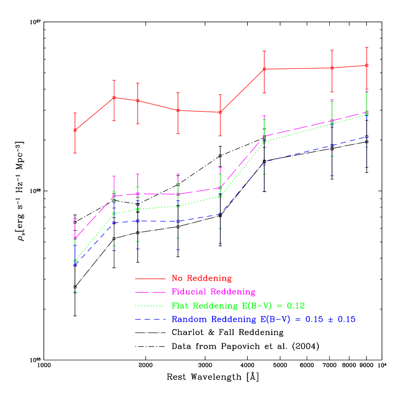
Figure 7.— The luminosity density of the universe for B-dropouts at $z\sim 4$ in the rest-frame UV to optical bands. The solid, red line gives the $\rho_{\nu}$ curve assuming no dust reddening; the magenta, long-dashed line assumes our fiducial reddening prescription; the green, dotted line assumes a uniform reddening for all galaxies; the blue, short-dashed line assumes a Gaussian distribution of $E(B-V)$ values (see text); the black dot-long-dashed curve assumes the Charlot & Fall (2000) reddening curve; and the black dot-short-dashed curve gives the observations from Papovich et al. (2004). The fiducial reddening prescription produces broad agreement with the observations while showing a small but interesting discrepancy in the observed H-band (see text for discussion).

With the expansive baseline in wavelength afforded by GOODS, we can construct a coarse average spectrum of LBGs by summing the flux densities of all the galaxies through each photometric band. The resulting SED is known as the “luminosity density” $\rho_{\nu}$, and can be used to study the average properties of the galaxy population. For example, Papovich et al. (2004) used this method to suggest that the universe’s stellar mass density increases by 33% between $z=4$ and $z=3$, and Rudnick et al. (2003) used it to infer that the density of stellar mass in massive galaxies grows by $10\times$ between $z=3$ and $z=0$.

We compute $\rho_{\nu}$ following the method of Papovich et al. (2004). We consider only those galaxies that satisfy the B-dropout color cuts, the brightness cut at $z_{850}<26.5$, and an additional brightness cut at $i_{775}<m^{*}(i_{775})+1$, where $m^{*}(i_{775})=25.74$ is derived from the value used in Papovich et al. (2004, which in turn was derived from Giavalisco et al. 2004b) by redshifting from $z=3.9$ to $z=4$. The flux densities of the selected galaxies in all relevant photometric bands are converted to luminosities, added, and divided by the simulation volume to produce the luminosity density $\rho_{\nu}$.

We compared the luminosity densities of the two simulations computed in this way as a further resolution check on the G6 simulation, using only galaxies whose stellar masses were in the range $9.7<\log(M_{*}/\mbox{M}_{\sun})<10.5$ since this range is resolved by both simulations (cf. Figure 3). We found that, for these galaxies, the D5 luminosity density is 81%–94% that of G6 at this redshift for the various bands. This is smaller than the uncertainty in each simulation owing to Poisson noise and cosmic variance, which we derive below, so we ignore this offset. Since neither of our simulations completely covers the mass range of interest, we compute the total luminosity density by summing the independent contributions from G6 galaxies with $\log(M_{*}/\mbox{M}_{\sun})\geq 9.7$ and D5 galaxies with $\log(M_{*}/\mbox{M}_{\sun})<9.7$.

We estimate uncertainty in $\rho_{\nu}$ using the jackknife method (Lupton, 1993; Zehavi et al., 2002; Weinberg et al., 2004). In general, the uncertainty in estimates of volume-averaged cosmological quantities such as the luminosity density $\rho_{\nu}$ receives independent contributions from Poisson noise and cosmic variance. One simple way to account for both effects is to divide up the sampled region into smaller subvolumes of comparable size, estimate $\rho_{\nu}$ in each volume, and take the variance in these estimates as the overall uncertainty. As Zehavi et al. (2002) have noted, this method tends to overestimate the error owing to cosmic variance on scales that are larger than the size of the subsamples. The jackknife method utilizes subsamples whose sizes are similar to that of the full sample. In this method, each subsample is obtained by excluding a small region (such as one octant of the simulation) from the full sample in turn and estimating $\rho_{\nu}$ in the remaining sample. The full uncertainty is then readily obtained from the formula:

$$\sigma^{2}(\rho_{\nu})=\frac{N-1}{N}\sum_{i=1}^{N}(\rho_{\nu,i}-\langle\rho_{\nu}\rangle)^{2}$$ (4)

where $N$ indicates the number of subsamples. We obtain the uncertainty in the $\rho_{\nu}$ for each simulation by computing jackknife errors over octant subsamples in this way and, when combining G6 and D5, we add the respective errors in quadrature (this is justified since the two simulations are run with different random number seeds and therefore provide independent measurements of the same quantity).

Figure 7 shows the result. The solid red line is obtained in a dust-free universe; the purple long-dashed, green dotted, and blue short-dashed lines use the Calzetti et al. (2000) reddening curve with our fiducial, flat, and random $E(B-V)$ distributions, respectively; the black dot-long-dashed curve uses the Charlot & Fall (2000) reddening prescription; and the black dot-short-dashed curve gives the data of Papovich et al. (2004). The Calzetti et al. (2000) curve is widely used, but the Charlot & Fall (2000) law is not yet as common despite its sound physical motivation. In its simplified form, it uses a $\lambda^{-0.7}$ reddening curve and attempts to account for the dusty environments around young stars by assuming that light from stars that are younger than the maximum age of their birth clouds (which we take to be $10^{7}$ years) has an optical depth to dust scattering that is greater than the optical depth for the older stars by some factor (which we take to be 3). For this curve, we took the normalization $A_{V}$ to be such that the “old” stars for each galaxy suffer the same extinction in rest-frame V as the entire population in our fiducial metallicity-derived case; the young stars are then at three times this optical depth.

It is clear that the fiducial reddening prescription produces broad agreement with the data from the rest-frame UV into the rest-frame optical. It is also not too different from the results of the other $E(B-V)$ distributions. In addition, for reasonable amounts of dust extinction, the shape of $\rho_{\nu}$ is not sensitive to the reddening prescription: all of the simulated curves show relatively flat UV and optical continua with a strong break at 4000 Å. We emphasize that the agreement between the data and the $\rho_{\nu}$ from our fiducial $E(B-V)$ distribution has not been enforced by hand; the fiducial distribution has only been calibrated against nearby late-type galaxies from SDSS.

While all of the simulated data points are affected by dust extinction, the points at 1200 Å (observed $V_{606}$) are suppressed by an additional $0.4\pm 0.1$ magnitudes ($\approx 25\%$) owing to IGM absorption, as noted in § 2.4. Meanwhile, the simulated points at 7200 and 9000 Å (observed [3.6] and [4.5]) are determined primarily by the stellar masses of the simulated LBGs with little dependence on dust attenuation. They are reasonably robust, and straightforwardly testable, predictions of our simulation.

It is interesting that the simulated luminosity density curve has a strong break at 4000 Å that is not visible in the data. The 4000 Å break results from a large number of metal absorption features at wavelengths $\lambda<4000$ Å acting in concert with the Balmer break at 3646 Å. As it occurs only in the spectra of relatively cool stars, it is visible only in stellar populations older than $\sim 100$ Myr and is widely used as a characteristic age indicator. The stellar populations in our galaxies have characteristic ages of 300 Myr (Figure 11); therefore a break is expected. Although star formation histories of LBGs are currently poorly constrained by observations, the work of Shapley et al. (2001) suggests that a substantial population of galaxies whose mean stellar ages are old enough to show a 4000 Å break should be visible by $z\sim 4$; thus, one might expect to see this feature in the data. The ingredients that are most likely to give rise to the discrepancy are redshift scatter, dust reddening, the simulated star formation histories, and uncertainty in the data. As the 4000 Å break is an important feature for characterizing stellar populations, we consider these possibilities in turn.

Redshift scatter is present in the data since the redshifts of LBGs are known only to within the width of the selection function resulting from the color cuts that are used to define the LBG sample. We find that the B-dropout color cuts select most galaxies with $3.5<z<4.5$ and very few galaxies outside this range; thus, the optical data in Figure 7 can be viewed roughly as a convolution of the unknown, correct luminosity density curve with a tophat function of width 400–900 Å, depending on the observed band. We tested whether this could remove the 4000 Å break by introducing artificial scatter of $\pm 0.5$ into the simulated galaxies’ redshifts before applying the B-dropout selection criteria and found that the simulated luminosity density dropped in normalization but did not change shape. The normalization drop results from moving galaxies into redshift ranges where the selection function is lower, and the 4000 Å break is unchanged because the width of the selection function is not broad enough to allow significant flux from redwards of the break to spill into the observed H band (rest-frame 3200 Å).

As always, dust reddening is a possibility. With enough dust any galaxy’s observed UV continuum can be reddened to the point that the 4000 Å break disappears. Unfortunately, if we add enough dust to our galaxies (using the  Calzetti et al. 2000 law with a reasonable intrinsic $E(B-V)$ distribution) that the shape of the simulated luminosity density curve approaches the observed shape, its normalization drops more than an order of magnitude below the observed normalization owing to too many galaxies being reddened out of the observed sample. Thus for this explanation to be viable, the real LBGs must be significantly more luminous and dustier than our simulated sample; observations in the [3.6] and [4.5] bands should constrain this possibility. An alternative check on the normalization is provided by the rest-frame UV luminosity function (§ 4.3), which shows broad agreement given our fiducial $E(B-V)$ distribution. Figure 7 thus tells us that the simulated 4000 Å break is insensitive to reddening over a variety of $E(B-V)$ distributions and two well-calibrated reddening curves if we wish to preserve agreement between the observed and simulated rest-frame UV luminosity functions. Hence, we do not think that reddening is the main cause although it may contribute.

Our currently favored explanation for the “missing” 4000 Å break is the uncertainty in the data of Papovich et al. (2004). Their sample was culled from $\approx 50$ square arcminutes of data (or $\approx 5\%$ of the comoving volume in our simulation) owing to the limited areal coverage of the VLT/ISAAC data, and their bootstrap uncertainties do not account for cosmic variance (note, however, that the break was not observed in their U-dropouts at $z\sim 3$ either). More insight into this problem could be gained if the luminosity density measurement were reproduced with the full GOODS data set including deep imaging in the critical VLT/ISAAC H-band.

4.3. Luminosity Functions

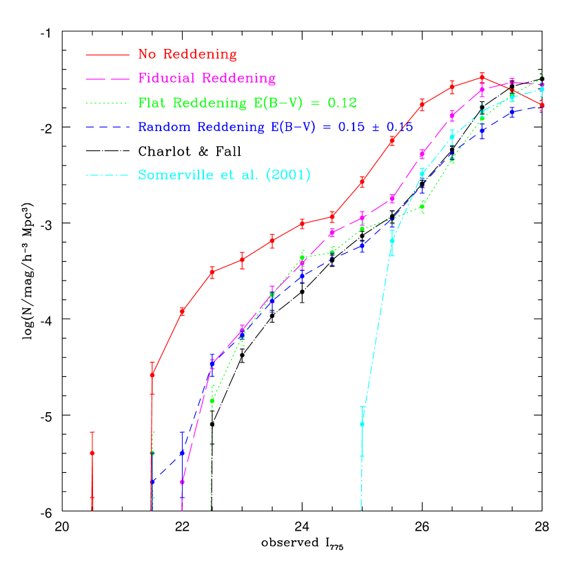
Figure 8.— The rest-frame UV LF of B-dropouts assuming various different $E(B-V)$ distributions. The solid red curve assumes no reddening; the dotted green curve assumes a uniform reddening; the short-dashed blue curve assumes a Gaussian distribution of $E(B-V)$ values (see text); the long-dashed magenta curve assumes our fiducial reddening prescription; the cyan dot-short-dashed curve assumes the $E(B-V)$ distribution of Somerville et al. (2001); the black dot-long-dashed curve assumes the Charlot & Fall (2000) reddening curve. For a variety of reasonable $E(B-V)$ distributions, the simulated LF varies by $\leq 2\times$ from the curve that assumes our fiducial $E(B-V)$ distribution.

In this section we present rest-frame UV and optical luminosity functions for the simulated B-dropout sample. Several studies of the luminosity functions of LBGs in these simulations have already been published. Nagamine et al. (2004a, b) found that the simulated luminosity functions at $z\sim 3$ in observed $V$ and $R$ reproduce the observed luminosity function at the bright end reasonably well while exhibiting steep slopes $\alpha\sim-2$ at the faint end. Night et al. (2005) performed a similar study for LBGs at $z$ = 4 – 6 and found good agreement between simulated and observed luminosity functions in $i^{\prime}$ and $z^{\prime}$ provided that Calzetti et al. (2000) reddening was assumed with $E(B-V)$ = 0.15 – 0.30. Additionally, they found a steep slope $\alpha\sim-2$ at the faint end of the simulated luminosity function. At the risk of some overlap with their work, we will present a complete discussion of the LBGs in these simulations under a single set of assumptions such as our mass cuts and assumed $E(B-V)$ distribution. In order to create a single luminosity function, we combine the results of the D5 and G6 simulations following the same method as described in § 4.2.

Reddening: Figure 8 shows the simulated $i_{775}$ luminosity function for a number different $E(B-V)$ distributions. The galaxies used in creating this plot satisfy the GOODS color cuts but do not necessarily satisfy the GOODS detection limit $z_{850}<26.5$. The solid red line shows the luminosity function derived if dust is absent so that $E(B-V)$=0. The magenta long-dashed, green dotted, and blue short-dashed lines show the luminosity function under the assumptions of a fiducial, flat, and random $E(B-V)$ distribution, respectively (§ 2); and the cyan dot-short-dashed line assumes that the reddening varies with star formation rate in the way described by Somerville et al. (2001). All of these curves use the Calzetti et al. (2000) reddening curve once the reddening $E(B-V)$ for each galaxy is chosen. The black long-dash-dotted line uses the Charlot & Fall (2000) reddening curve as described in § 4.2.

We briefly consider the various reddened curves in turn. Inspection reveals slight differences between the results from the flat, random, and fiducial $E(B-V)$ distributions. Our fiducial $E(B-V)$ distribution naturally produces a weak positive correlation between stellar mass and reddening that is absent in the random distribution, preferentially reddening massive galaxies out of the sample (cf. Figure 6). For the same reason, at the faint end the random $E(B-V)$ distribution causes more galaxies to be reddened out of the sample than the fiducial distribution. The random distribution allows a few more bright galaxies to have low dust content than either the flat or fiducial $E(B-V)$ distributions. The curve from the flat distribution is similar to the others except at the bright end, where, once again, the redder intrinsic colors cause these galaxies to be preferentially reddened out of the sample if high reddening is enforced. Despite these minor differences, it is clear that the random, fiducial, and flat $E(B-V)$ distributions produce qualitatively similar results. The curve derived from the Somerville et al. (2001) $E(B-V)$ distribution reddens rapidly star-forming galaxies out of our sample far too effectively; it is clearly not appropriate for our simulated galaxies. The curve derived from the Charlot & Fall (2000) reddening prescription has almost exactly the same shape as our fiducial curve but is fainter by roughly 0.5 magnitude; this is the result of adding extra extinction to the youngest stars in each galaxy. It would not be difficult to modify the parameters we used for the Charlot & Fall (2000) law to obtain better agreement, but as little insight would be gained from this exercise, we do not do so.

As with the observed mass fraction, the dominant source of uncertainty in these predictions is clearly the unknown form of the intrinsic $E(B-V)$ distribution and reddening curve in high-redshift galaxies. However, the important point is that the overall shape of the simulated luminosity function is fairly insensitive to the details of the reddening procedure such that reasonable distributions agree to within a factor of 2. This gives us further confidence that our fiducial $E(B-V)$ distribution will yield useful predictions.

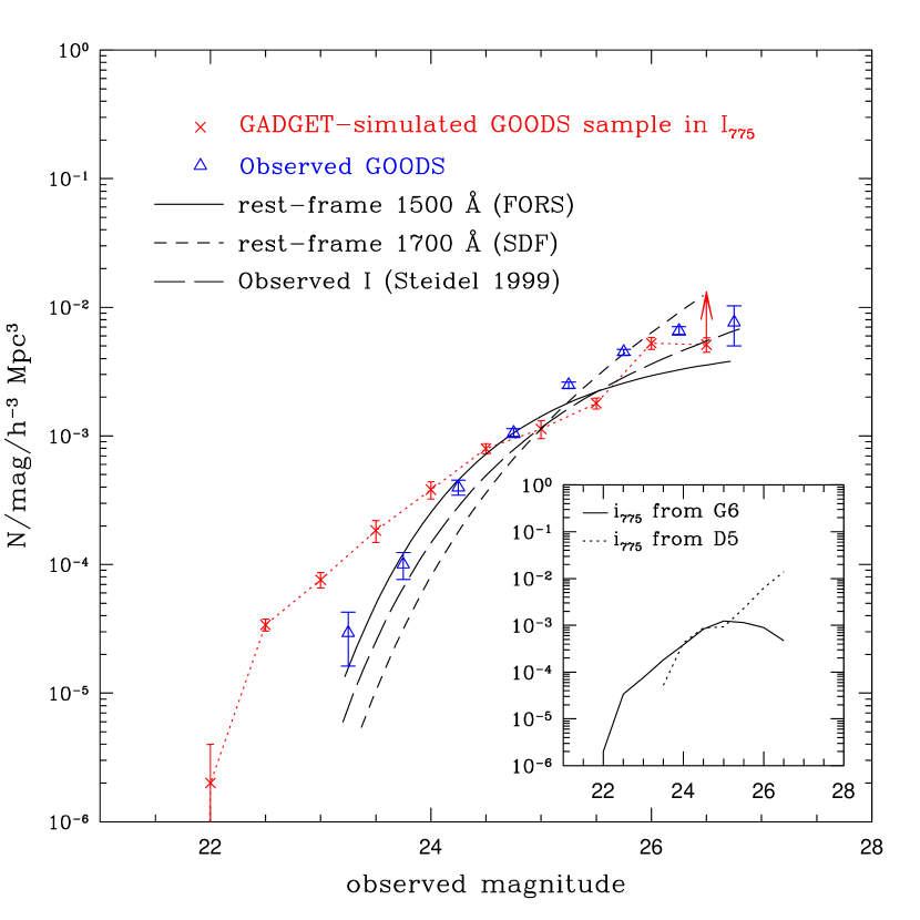
Figure 9.— (large) The simulated rest-frame UV LF of B-dropouts (assuming our fiducial reddening prescription) compared with several published curves and the GOODS data. Red crosses indicate the simulated LF in observed $i_{775}$; the arrow points to the value of the LF at that point if the brightness cut in $z_{850}$ is relaxed. Errors in the simulated plot are from jackknife resampling. LFs from the FORS survey (Gabasch et al., 2004) at rest-frame 1500 Å, the Subaru Deep Field (Ouchi et al., 2004) at rest-frame 1700 Å, and Steidel et al. (Steidel et al., 1999) in observed $I$ are indicated by solid, short-dashed, and long-dashed curves, respectively, and were derived from the literature as described in the text. The GOODS B-dropout sample of Giavalisco et al. (2004b) in observed $i_{775}$ is indicated by blue triangles. (inset) The LFs of the D5 and G6 simulations, which were combined to produce the full curve as described in the text. The simulated LF assuming our fiducial $E(B-V)$ distribution produces broad agreement with available constraints, with a possible excess at the bright end (see text for discussion).

Comparison to Observations: Figure 9 shows a comparison of the simulated $i_{775}$ luminosity function using the fiducial $E(B-V)$ distribution with various observational results. The red crosses with jackknife errors indicate the simulated GOODS sample, while the arrow at the faint end points to the value obtained by relaxing the brightness cut $z_{850}<26.5$. The plot also includes observed LFs from the FORS survey (Gabasch et al., 2004) at rest-frame 1500 Å, the Subaru Deep Field (Ouchi et al., 2004) at rest-frame 1700 Å, and Steidel et al. (Steidel et al., 1999) in observed $I$; these are indicated by solid, short-dashed, and long-dashed curves, respectively. The FORS LF was constructed at $z=4$ using the fitting function given by Equation 1 and the values given by Table 4 in Gabasch et al. (2004). The Steidel et al. $z\sim 4$ LF was constructed from the updated Schechter parameters for U-dropouts ($z\sim 3$) given in Adelberger & Steidel (2000) and following the method described in Steidel et al. (1999): we used a distance modulus to shift $m_{*}$ from $z=3.04$ to $z=4.0$, multiplied the normalization $\phi_{*}$ by 80%, and left $\alpha$ constant, yielding ($\phi_{*}$, $m_{*}$, $\alpha$) = ($3.52\times 10^{-3}$, 25.02, -1.57). The Subaru Deep Field LF is the LF for $BRi$-LBGs from Table 4 of Ouchi et al. (2004), where we have used their derived faint-end slope $\alpha=-2.2$. Note that because the effective wavelengths of the bands used in these surveys as well as the mean redshifts of their LBG samples differ, offsets of 0.1–0.3 magnitudes between their reported LFs do not necessarily indicate disagreements.

The observed and theoretical GOODS LFs both flatten out for magnitudes fainter than 26. By contrast, the magnitude-unlimited GOODS luminosity function seems to turn over at a fainter magnitude. In fact, this turnover owes to the conservative cut in stellar mass: The more we relax this restriction, the fainter the magnitude at which the rest-frame UV luminosity function turns over. Hence, our simulation is predicting an extremely steep intrinsic faint-end slope ($\alpha\sim-2$) that cannot be observed in B-dropout samples of GOODS depth.

LBGs brighter than 25th in $i_{775}$ also seem to be overproduced in the simulation. This is analogous to the bright-end excess noted in the same simulation at $z=2$ by Nagamine et al. (2005a). The excess could result from any of four possibilities: (1) incorrect prescription for dust reddening; (2) lack of truncation of star formation, owing to e.g. feedback from black hole growth; (3) overmerging; and (4) incorrect feedback model for star formation. We consider each of these possibilities in turn, as they provide interesting insights into high-redshift galaxies.

The first possibility is consistent with the idea, noted by Shapley et al. (2001) and others, that dust extinction correlates with luminosity, and hence in our model, star formation rate. Clearly, if our assumed extinction scaled more strongly with star formation rate, closer to that in Somerville et al. (2001), then the discrepancy would be alleviated. Evidence in support of this possibility is provided by Daddi et al. (2004): For their actively star-forming $BzK$ sample at $z>\sim 1.4$ with $K<20$, they find a median star formation rate of $200\;\mbox{M}_{\sun}\mbox{ yr}^{-1}$ and a median reddening of $E(B-V)\sim 0.4$. Indeed, Nagamine et al. (2005b) found that the simulations can reproduce the comoving number density of Extremely Red Objects (EROs) at $z=$ 1–2 if a uniform reddening of $E(B-V)=0.4$ is assumed for the entire simulated sample. Using our fiducial $E(B-V)$ distribution, simulated galaxies at $z=4$ with star formation rates between 150 and 250 $\mbox{M}_{\sun}\mbox{ yr}^{-1}$ suffer a significantly weaker median reddening of roughly 0.15. Additionally, we note that some of the most massive, rapidly star-forming galaxies could correspond to extremely dusty starbursts that are observed as sub-millimeter sources (Chapman et al., 2004), as we will consider further in § 5.4. Recent observations suggest that the effects of dust on these and other massive galaxies ($\log(M_{*}/\mbox{M}_{\sun})>11$) may not even follow simple foreground screen attenuation laws such as that of Calzetti et al. (2000) (Chapman et al. 2005; Papovich et al. 2005, in preparation). In this case, the Charlot & Fall (2000) reddening curve is almost certainly more appropriate; unfortunately, observations to date have not constrained the parameters needed to use it at high redshift.

The second possibility is that our simulation may fail to account for some mechanism that suppresses or truncates star formation in real galaxies. In this case, the bright-end excess is an early sign of the difficulties that are commonly seen in cosmological simulations and SAMs (Somerville, 2004; Nagamine et al., 2005a). Upcoming work incorporating AGN feedback may help with this (Di Matteo et al., 2005; Springel et al., 2005a, b).

The third possibility is overmerging owing to poor spatial resolution. Figure 3 shows that galaxies with stellar masses $\log(M_{*}/\mbox{M}_{\sun})<10.25$ are slightly underrepresented in the G6 simulation relative to the D5. Owing to its poorer spatial resolution, galaxies that form in the G6 are more extended than in D5, rendering them more susceptible to tidal disruption and subsequent accretion by more massive galaxies. Massive galaxies in G6 then grow more rapidly than they would in a higher-resolution simulation, leading in principle to a brighter characteristic magnitude M^∗. The impact of overmerging on the bright end of a rest-frame UV LF can be characterized by inspecting the galaxy mass function at the massive end. Figure 3 shows that, up to the maximum galaxy mass produced in the smaller, higher-resolution D5 simulation, the mass functions of the D5 and G6 simulations agree quite well. Together with the evidence that the birthrates in the G6 are numerically resolved (Figure 4), this gives us confidence that overmerging is not the dominant source of the discrepancy.

The final possibility is an incorrect model for supernova feedback. In particular, our simulation’s prescription for kinetic feedback endows all galactic outflows with a common velocity, 484 km s^-1. This may be an oversimplification. For example, Martin (2005) found that outflow velocities in a sample of 18 ultraluminous infrared galaxies correlate well with star formation rate, and suggested that this may result in winds more effectively suppressing star formation in massive galaxies.

In summary, our study of the rest-frame UV LF confirms the previously cited studies in the following respects: (1) the simulated and observed LFs show broad agreement when a reasonable amount of dust extinction is assumed; (2) the intrinsic faint-end slope of the simulated LF is $\sim-2$; and (3) an excess at the bright end of the simulated LF suggests that more work is required to understand the effects of star formation and AGN feedback as well as dust reddening on massive galaxies. The fact that our work reproduces these results despite our having employed a different group finder and a more physically-motivated prescription for dust reddening suggests that these results are robust to the analysis procedure.

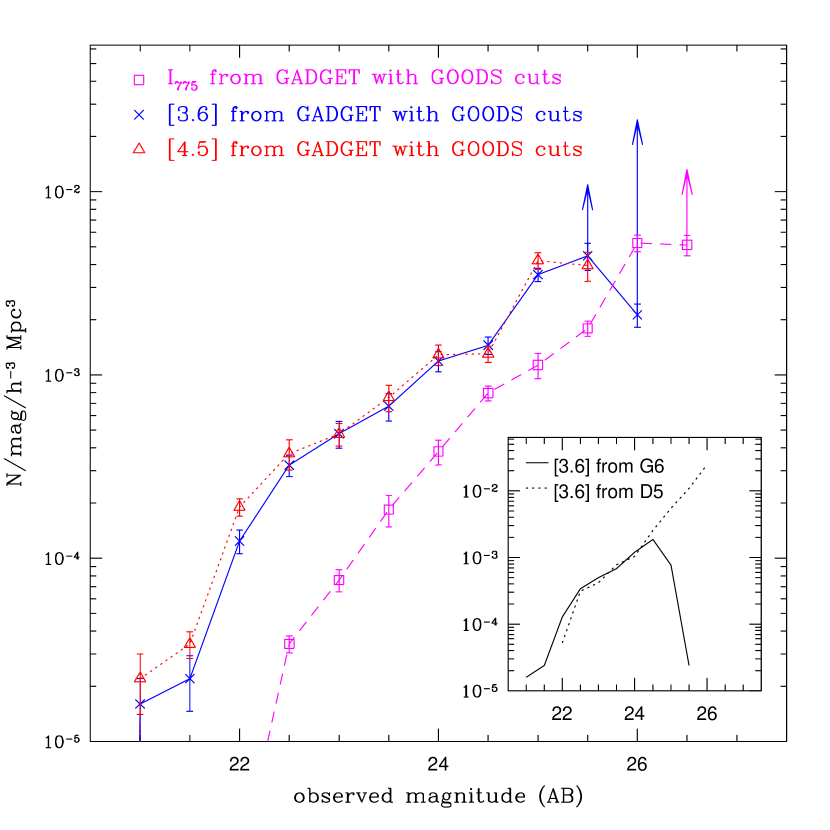
Figure 10.— (large) The simulated rest-frame UV and optical LFs of B-dropouts. The arrows point to the values of the LF if the brightness cut in $z_{850}$ is relaxed. Errors are from jackknife resampling. (inset) The luminosity functions of the D5 and G6 simulations in observed [3.6], which were combined to produce the top curve as described in the text. The rest-frame optical LF is very similar to the rest-frame optical LF, shifted roughly 1–2 magnitudes brighter.

Figure 10 shows the rest-frame optical luminosity functions and compares them with the rest-frame UV luminosity function. The observed [3.6] and [4.5] luminosity functions are very similar, suggesting that measurements of stellar mass may readily be made in the more sensitive [3.6] channel. Since LBGs tend to be 1–2 magnitudes brighter in rest-frame optical than in rest-frame UV, the rest-frame optical luminosity function is essentially the same as the rest-frame UV luminosity function, shifted 1–2 magnitudes brighter. This is consistent with the trend, discussed below, that LBGs are simply the most massive of the early galaxies, and that their star formation rates correlate with their masses. A closer look suggests that the rest-frame UV luminosity function appears to be slightly steeper than its optical counterpart, consistent with the tendency for more massive galaxies to be redder. The simulations predict that the faint end of the intrinsic luminosity function is essentially a power-law down to much fainter masses than GOODS can observe; the turnover in the intrinsic luminosity function at [3.6] $\approx 26.5$ owes to the 64 star particle mass resolution cut. Similarly, the turnover in the observed luminosity function at [3.6] $\approx 25$ results directly from the GOODS magnitude cut at $z_{850}<26.5$ and translates into a mass cut at $\log(M_{*}/\mbox{M}_{\sun})\approx 9.5$ (Figure 12; see also Figure 6).

5. COMPARING PHYSICAL AND PHOTOMETRIC PROPERTIES OF LBGs

In this section we focus on correlations between the properties of the simulated sample, comparing to the data wherever possible. Unless otherwise noted, we employ our fiducial, metallicity-derived $E(B-V)$ distribution with the Calzetti et al. (2000) reddening curve. We occasionally compare the physical properties of our simulated sample at $z=4$ with the properties derived from observations at lower redshift $z\sim 3$ since LBGs at this epoch are well-studied. This may not be a valid comparison since some evolution may occur in the population of star-forming galaxies between these two epochs (e.g., Papovich et al., 2004). On the whole, however, the two populations are expected to be very similar (Steidel et al., 1999); thus, we proceed while noting that factor of 2 differences do not necessarily suggest a failing of the simulation.

5.1. Physical Properties

Figure 11.— Physical properties of B-dropouts versus stellar mass. (top) instantaneous star formation rate; (second) median age of the star particles; (third) mean metallicity of the star particles; (fourth) local density of observable stellar mass, relative to the mean. Red points and blue crosses denote G6 and D5 galaxies, respectively. The contours enclose 63% and 95% of the simulated galaxies. The histograms and contours are constructed by volume-weighting the contributions of the D5 and G6 samples as described in the text. Note the strong correlation between star formation rate and stellar mass.

Figure 11 shows a number of physical correlations in addition to the basic properties of the simulated GOODS $z\sim 4$ sample. Red points and blue crosses denote G6 and D5 galaxies, respectively. The break in the G6 sample at $\log(M_{*}/\mbox{M}_{\sun})=9.64$ owes to our 64 star particle cut. The histograms are constructed by considering only G6 galaxies more massive and D5 galaxies less massive than $\log(M_{*}/\mbox{M}_{\sun})=9.7$ and weighting the contribution from the D5 galaxies by the ratio of the simulation volumes. The contours were constructed using the same method and define regions enclosing 63% and 95% of the galaxies. For each galaxy, $\log(M_{*}/\mbox{M}_{\sun})$ is the sum of the masses of the star particles; the star formation rate is the instantaneous star formation rate; $t_{*}$ is the median age of its star particles; $12+\log(O/H)$ is the mean metallicity of its star particles; and $\rho/\overline{\rho}$ is the local space density of stellar mass in B-dropouts (roughly equivalent to an optical luminosity-weighted number density), normalized by the mean over the simulation volume. We compared instantaneous star formation rates with star formation rates obtained by averaging over the last 100 Myr and found that they are within a factor of 2 (§ 5.4), in agreement with Weinberg et al. (2002).

Stellar Mass: The stellar masses of our sample fall predominantly in the range $\log(M_{*}/\mbox{M}_{\sun})=$ 9–10 with a peak in the range 9.5–9.8 and a significant tail out to $\log(M_{*}/\mbox{M}_{\sun})\approx 11$. The falloff at lower masses owes entirely to the brightness cut at $z_{850}<26.5$ (cf. Figures 5 and 3). Overall, this range is slightly more massive than the sample from the semi-analytic model of Idzi et al. (2004, Figure 2); in particular, those semi-analytic models do not reproduce our high-mass tail. Papovich et al. (2001) used population synthesis techniques to infer the properties of the stellar populations of 33 LBGs in the HDF-N between $z\sim 2$ and $z\sim 3.5$ and found a typical stellar mass of $10^{10}\mbox{M}_{\sun}$. Shapley et al. (2001) used similar techniques to infer the properties of 74 fairly bright LBGs at $z\sim 3$ and found masses in the range $\log(M_{*}/\mbox{M}_{\sun})=$ 9–11 with a median at $1.2\times 10^{10}h^{-2}\mbox{M}_{\sun}$. While these measurements are somewhat more massive than the median in Figure 11, we note that both of these samples are biased towards brighter and thus more massive galaxies than our simulated GOODS sample. Also, given that Papovich et al. (2004) report a $\sim 33\%$ buildup of stellar mass between $z=4$ and $z=3$, it is reasonable to suppose that galaxies at $z=3$ might be more somewhat more massive than galaxies at $z=4$. Thus, we conclude that our LBG model seems to be able to match the distribution of observed stellar masses.

Star Formation Rates: The bulk of the observed galaxies are forming stars at rates of 1–10 $\mbox{M}_{\sun}\mbox{ yr}^{-1}$. A small active population is forming stars at aggressive rates of $100\sim 1000\;\mbox{M}_{\sun}\mbox{ yr}^{-1}$ with the median instantaneous star formation rate of the ten most rapidly star-forming galaxies being $\sim 450\;\mbox{M}_{\sun}\mbox{ yr}^{-1}$.

Our models produce a tight correlation between stellar mass and star formation rate, as noted elsewhere in hydrodynamic simulations (e.g., Davé et al., 1999; Weinberg et al., 2002; Nagamine et al., 2004a). A fit to this relation for our simulations gives

$$\log(\dot{M}_{*}/\mbox{M}_{\sun})\approx 1.14\log(M_{*}/\mbox{M}_{\sun})-10.2,$$ (5)

which is shown in the plot. As mentioned in § 3, a comparison of the mass functions (Figure 3) and the birthrates (not shown) of the D5 and G6 galaxies suggests that the G6 galaxies may be suffering slightly from overmerging, but we believe that the star formation rates in the G6 simulation cannot be overpredicted by more than a factor of 2, which is comparable to the intrinsic scatter. Figure 11 thus predicts that a few galaxies with instantaneous star formation rates of 500–1000 $\mbox{M}_{\sun}\mbox{ yr}^{-1}$ may fall within the GOODS field. According to our prescription for dust reddening, they should all be observable as LBGs; however, considering observational evidence that the most massive galaxies may not obey the Calzetti et al. (2000) reddening curve (Chapman et al. 2005; Papovich 2005, in preparation), this may not be the case in reality. We will return to these massive star formers in § 5.4. For now, the strong correlation between stellar mass and star formation rate implies that LBGs observed at $z=4$ are predominantly massive galaxies.

The scatter in the plot of instantaneous star formation rate versus stellar mass can be regarded as a measure of the star formation rate “burstiness” as a function of stellar mass. For example, galaxies with stellar mass of $10^{10}\;\mbox{M}_{\sun}$ have star formation rates between 10 and 30 $\mbox{M}_{\sun}\;\mbox{yr}^{-1}$. This means that such a galaxy will, on average, tend to form 10 $\mbox{M}_{\sun}\;\mbox{yr}^{-1}$ although it will sometimes experience bursts of up to 30 $\mbox{M}_{\sun}\;\mbox{yr}^{-1}$; if the simulation produced more dramatic bursts than this then there would be more spread in the plot. Note, however, that the simulation does not adequately resolve merger-driven starbursts (e.g. Hernquist & Mihos 1995; Mihos & Hernquist 1996; Springel et al. 2005b). For those galaxies undergoing mergers, the instantaneous star formation rate reported by the simulation may be an underestimate even though the total stellar mass formed by the end of the merger event is reliable. Relatedly, Weinberg et al. (2002) notes that there could be merger events between galaxies not massive enough to be resolved in the simulation, which cause them briefly to be luminous enough to satisfy the B-dropout magnitude cuts. However, the broad agreement between the simulated and observed rest-frame UV luminosity functions suggests that the bulk of the LBG population can be accounted for without resorting to such phenomena.

The lower end of the distribution of star formation rates is reasonably consistent with semi-analytic results (Somerville et al., 2001; Idzi et al., 2004). However, the space density of more rapidly star-forming galaxies 10–100 $\mbox{M}_{\sun}\mbox{ yr}^{-1}$ is higher in our results, no doubt owing to the drastically different star formation and reddening prescriptions involved. Observationally inferred LBG star formation rates are in reasonable agreement with our results (Shapley et al., 2001; Papovich et al., 2001). The histogram of star formation rates in Shapley et al. (2001) seems to show a higher space density of galaxies with star formation rates greater than $10\;\mbox{M}_{\sun}\mbox{ yr}^{-1}$, but since this sample was hand-selected to span the range of possible properties of LBG stellar populations rather than to satisfy an unbiased selection criterion, such an excess of galaxies exhibiting more extreme properties is unsurprising.

Metallicity: The simulated galaxies’ stellar metallicities correlate tightly with stellar mass. The simulation computes metallicities by allowing the metallicity of a star-forming gas particle to increase during each timestep in proportion to its current star formation rate and a constant yield that is set to the solar metallicity 0.02; as mentioned, a star particle inherits the metallicity of its parent SPH particle. Given that a galactic mass-metallicity relation is not assumed in this prescription, it is of interest to examine the trend that nonetheless results. Such a trend is required by a growing body of observational evidence (e.g., Lequeux et al. 1979, Garnett & Shields 1987, Tremonti et al. 2004); for a review of this subject see the discussions in Tremonti et al. (2004).

The dashed line gives the median relation between stellar mass and gas-phase metallicity observed by Tremonti et al. (2004) in their sample of $\sim 53,000$ nearby ($z\approx 0.1$) star-forming galaxies. Despite the simple prescription for enrichment, the slope of the trend in the simulated sample shows excellent agreement with the observed low-redshift trend. Over a range of two orders of magnitude in stellar mass, the simulated galaxies show a stellar metallicity that is roughly 0.6 dex below the low-redshift value for their respective stellar masses and the most massive objects ($\log(M_{*}/\mbox{M}_{\sun})\geq 11$) already exhibit solar metallicity. Closer examination suggests that the simulation may not produce the flattening observed by Tremonti et al. (2004) at stellar masses greater than $\log(M_{*}/\mbox{M}_{\sun})=10.5$. While such a disagreement may be a failing if observed in gas-phase metallicities at low redshift, it is not necessarily a failing for stellar metallicities at high redshift.

Physical processes that could contribute to the observed mass-metallicity relation include selective removal of metals by supernova-driven winds (“depletion,” first modeled by Larson 1974 and favored by Tremonti et al. 2004), ISM enrichment owing to supernova feedback (“astration,” Lequeux et al., 1979), dilution owing to infall of unenriched gas, and late-time return of relatively unenriched gas to the ISM from evolved, low-mass stars (“recycling”). Of these processes, depletion contributes in the simulation via the superwind prescription, astration is built into the enrichment prescription, dilution can contribute, and recycling is not accounted for. If astration dominated the trend then the stellar metallicities in all simulated galaxies would be expected to be roughly solar owing to the constant yield assumed by the star-formation prescription. If dilution dominated the trend then massive galaxies, which are accreting gas much more rapidly than less massive galaxies, would be expected to exhibit lower metallicities—the opposite of what is seen. Thus, the simulation’s superwind prescription is the most likely cause of the stellar mass-metallicity relation, and the excellent agreement between the slopes of the observed and simulated relations give us further confidence in the superwind prescription as well as in the predicted LBG metallicities.

Median Age: Figure 11 (second panel) shows that the median age of a galaxy’s stars is at best weakly correlated with stellar mass. This means that the phenomenon of “downsizing” (Cowie et al., 1996), i.e. that larger galaxies are observed to have an older stellar population out to $z\sim 1$, is at best weakly evident in our models at $z=4$. This is a fundamental and testable prediction of our simulations.

The age distribution extends from 200–600 Myr with a median around 350–400 Myr. This is roughly a factor of 2 older than the population in the semi-analytic simulations of Idzi et al. (2004), consistent with the picture in which LBGs are massive galaxies rather than starbursts. These values are also roughly a factor of two older than the constraints derived from observed LBGs at $z\sim 3$ by Shapley et al. (2001). However, the uncertainties in star formation histories derived via this technique are substantial (Shapley et al., 2001, 2005); thus, agreement within a factor of two gives us confidence that our models have reasonably realistic star formation histories.

Environment: The fourth panel gives the galaxy density $\rho/\bar{\rho}$ in each galaxy’s local environment. We define the density for each galaxy as the local density (relative to the mean) of stellar mass in the 16 nearest galaxies that would be observable by GOODS, smoothed with an SPH kernel; this is broadly equivalent to a number density weighted by rest-frame optical luminosity. There is a weak correlation between stellar mass and local matter density in the sense that the most massive galaxies are in denser environments. Galaxies in denser areas also show redder colors and higher star formation rates (Figure 12), likely arising as a secondary correlation owing to the tight relationship between stellar mass and star formation rate. Although there is considerable scatter, such a correlation might be observable in the GOODS sample. We note that weighting by stellar mass (or, equivalently, rest-frame optical flux) is critical; when we compute densities using unweighted number counts these weak trends disappear altogether.

5.2. Physical Versus Photometric Properties

Figure 12.— Physical versus photometric properties of B-dropouts. Solid contours enclose 63%, 86%, and 95% of the galaxies assuming our fiducial $E(B-V)$ distribution; dotted contours assume a dust-free universe. Contours are constructed by volume-weighting the contributions of the D5 and G6 simulations as described in the text. The dashed lines in the plot of stellar mass versus [3.6] flux show constant mass-to-light ratio corresponding to 1/8 (brightest), 1/4 (middle), and 1/2 (dimmest) of the solar value. Note that star formation rate correlates more strongly with optical flux than with UV flux, even when reddening has not been applied.

Figure 12 compares some physical and photometric properties of the simulated sample as it would be observed with reddening (solid contours) and without (dashed contours). Physical properties include stellar mass, star formation rate, age, and local galaxy density. Photometric properties include rest-frame UV ($V_{\rm 606}$) and optical ($[3.6]$) magnitudes, a short-baseline rest-UV color ($V_{\rm 606}-z_{\rm 850}$) and a long-baseline UV-optical color ($V_{\rm 606}-[3.6]$). While the GOODS measurements cover all four IRAC channels, we plot only the [3.6] band here because the [3.6] band will detect the largest fraction of the B-dropouts (§ 4). We note that the trends observed in [3.6] persist in the redder bands. Figure 12 shows the following interesting properties:

– Rest-frame optical data are a better predictor of star formation rate (SFR) than rest-frame UV data. This seems surprising at first, but is expected given the tight stellar mass-star formation rate correlation in Figure 11 along with the fact that reddening introduces much more scatter into the UV than into optical light. One may wonder whether rest-frame UV would be a better predictor of SFR if it were possible to remove the effects of reddening accurately; the dotted contours in Figure 12 suggest that this would at best allow UV flux to be an equivalently good predictor, but not better.

– The tight correlation between star formation and stellar mass also gives rise to a correlation between rest-frame UV flux and stellar mass, in qualitative agreement with the trend noted in U-dropouts at $z\sim$2–3.5 by Papovich et al. (2001). Shapley et al. (2005) do not find such a correlation in their UV-selected sample at $z\sim 2$. However, Papovich et al. (2005, in preparation) find a significant correlation between stellar mass and star formation rate in their sample of near-infrared–selected galaxies at $z\sim$ 1–3.5. Thus, a careful assessment of selection biases is probably necessary for determining whether the Shapley et al. (2005) result is in conflict with the simulations.

– More massive galaxies are redder in both the unreddened and reddened cases, with the trend accentuated in the reddened case because higher mass galaxies tend to have more dust. This trend is qualitatively consistent with observations (e.g. Papovich et al., 2001). It also leads to the counter-intuitive albeit weak trend that more rapidly star-forming galaxies are redder. Unfortunately, this correlation is not visible in the photometry (substituting a rest-frame UV magnitude for the star formation rate) if the scattering effects of reddening have not been removed.

– There are no obvious correlations between any photometric measurement and the galaxies’ stellar ages, consistent with the findings of Papovich et al. (2001) and Shapley et al. (2001) that star formation history is difficult to constrain from photometry alone.

– There is a very strong correlation between stellar mass and rest-frame optical magnitude, as expected. This correlation persists in the longer-wavelength IRAC bands (not shown) but the scatter does not decrease dramatically. We note that the correlation between optical flux and stellar mass in the G6 simulation at $z=2$ has previously been shown to agree well with observations (Nagamine et al., 2005b).

– The dashed lines in the figure of $M_{*}$ vs. [3.6] show lines of constant mass-to-light ratio corresponding to 1/8 (brightest), 1/4 (middle), and 1/2 (dimmest) of the solar value in this band. Evidently, the stellar populations of B-dropouts have roughly 1/4 the solar mass-to-light ratio in rest-frame optical light. For comparison, an unreddened SSP of the same metallicity with ages between 200 and 600 Myr has rest-frame V-band mass-to-light ratios of 0.12 to 0.24. The difference between the two ranges owes entirely to reddening: As the dashed contours in Figure 12 reveal, the mass-to-light ratios for the unreddened galaxies fall neatly within the range given by the SSPs. The agreement further indicates that the galaxies’ spectra are not dominated by bursts.

– There is a weak trend between color and environment in the sense that redder galaxies are in more overdense areas, and the trend between stellar mass and environment does translate into a trend between luminosity and environment. It will be interesting to see if stronger correlations are seen in the data; the ones predicted here will be quite difficult to pull out of the GOODS sample given additional scatter from photometric errors (which we have not included).

5.3. Photometric Properties

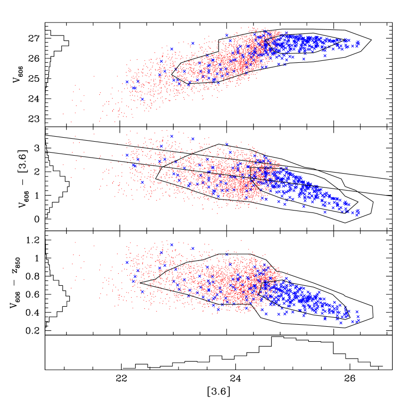
Figure 13.— Photometric properties of B-dropouts versus observed flux in [3.6]. (top) rest-frame UV; (second) rest-frame UV-optical color; (third) rest-frame UV color. The solid lines give possible color cuts for defining a high-redshift red sequence (see text). The contours enclose 63% and 95% of the simulated galaxies. The histograms and contours are constructed by volume-weighting the contributions of the D5 and G6 samples as described in the text. Rest-frame optical and UV flux show a strong correlation.

In this section we make predictions for observable photometric relationships for GOODS galaxies. Validating these predictions would lend support to our model for high-redshift galaxies, while disagreements would hopefully give insights into physical processes that are absent from the simulations. Figure 13 shows a short-baseline color, a long-baseline color, and a rest-frame UV magnitude plotted against a rest-frame optical magnitude ([3.6]). The following properties are evident:

– There is a strong positive correlation between rest-frame UV and optical flux, consistent with the relationship that the more massive galaxies are more rapidly star-forming (Figure 11). This is a fundamental prediction of our simulations, although the predicted scatter may be underestimated if starbursts that cannot be resolved by these simulations are prevalent.

– There is a strong correlation between the optical flux and color for both long-baseline (UV-optical) and short-baseline (UV-UV) colors. Since redder colors indicate a lower specific star formation rate, the simulations are reproducing the important trend in galaxy evolution noted in Papovich et al. (2001).

– We identify no passively-evolving, “red and dead” massive galaxies in our $z=4$ sample. At lower redshifts, such galaxies appear in a tight “red sequence” in color-magnitude diagrams (Bell et al., 2004). There is as yet no evidence for a red sequence at high redshifts $z\gtrapprox 1$ although several massive, passively evolving galaxies have been identified (Papovich et al. 2005, in preparation; Yan et al. 2004;  Daddi et al. 2005; Labbé et al. 2005). In any case, the color-magnitude diagrams in Figure 13 are clearly not bimodal. Indeed, this dearth of passively evolving massive systems is seen at lower redshifts in models as well, and highlights an important failure of current galaxy formation models (Somerville, 2004; Nagamine et al., 2005a). Therefore it is of interest to predict where red sequence galaxies might lie on these plots if they existed at high redshift.

Using $\sim 25,000$ galaxies from the COMBO-17 Survey, Bell et al. (2004) identified a color criterion for isolating red sequence galaxies and showed how the population’s colors evolve from $z=0.2\rightarrow 1.1$. One limit on the color of the $z=4$ red sequence is obtained by assuming that the red sequence does not evolve between $z=4$ and $z=1.1$. Using the color limit of  Bell et al. (2004) at $z=1.1$, and converting the rest-frame $U-V$ color and absolute $V$ magnitude to the observed $V_{606}-[3.6]$ color and observed [3.6] magnitude, gives the upper line in the plot of [3.6] versus $V_{606}-[3.6]$. On the other hand, since roughly 4 Gyr pass between $z=4$ and $z=1.1$ in our cosmology, we expect that the color of the hypothetical red sequence will be different at $z=4$. By assuming that the color evolves linearly with time we obtain an upper limit to the amount of color evolution experienced by the red sequence, shown by the lower line. Both lines succeed in isolating a sample of fairly massive red galaxies in the reddened sample. However, these galaxies are all forming stars at more than 1 $\mbox{M}_{\sun}\mbox{ yr}^{-1}$ and are red owing to dust, not low birthrates; if dust is removed then very few of the simulated galaxies are redder than either cut. The existence of dust-free massive red galaxies at these epochs, if found, would be a strong challenge for current models of galaxy formation.

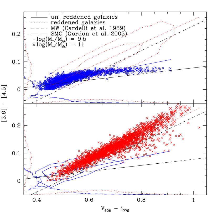
Figure 14.— Rest-frame optical versus UV color of B-dropouts from the G6 simulation assuming fiducial reddening (red) and no reddening (blue). Contours enclose 63% and 95% of the galaxies. Point size scales linearly with $\log(M_{*}/\mbox{M}_{\sun})$ as indicated. (top) reddened LBGs are given by the contour, unreddened LBGs are given by crosses; (bottom) reddened LBGs are given by crosses, unreddened LBGs are given by the contours. The solid, dotted, short-dashed, and long-dashed lines give regression fits to locus of B-dropouts assuming no reddening, fiducial reddening, a Milk Way reddening curve, and the SMC bar reddening curve. The slope of the color-color plot varies with the reddening curve and the median color varies with the typical amount of dust in the galaxies.

Figure 14 illustrates how ACS and IRAC data from GOODS may be used to constrain both the amount and form of reddening. We have produced photometry for two simulated GOODS samples from the G6 simulation, one in which there is no dust reddening and one in which there is substantial dust reddening. In the top panel of Figure 14, the blue crosses represent the unreddened LBGs while the red contours enclose 63% and 95% of the reddened LBGs; in the bottom panel the red crosses represent the reddened LBGs while the blue contours enclose 63% and 95% of the unreddened LBGs. The point sizes are scaled to the logarithm of the stellar mass as indicated. The histograms on the side show the normalized distributions of colors for each sample. The unreddened sample consists of a dense “blue clump” along with a diffuse “red tail” of low-mass galaxies whose optical color is nearly independent of UV color. In the reddened sample the “blue clump” has been spread out along the direction of the reddening vector—which results directly from the reddening curve employed (Calzetti et al., 2000)—and many of the “red tail” galaxies have been reddened out of the sample.

Roughly, the median colors can be calibrated to yield the typical dust extinction. Furthermore, the slope of the regression fit tells about the reddening law itself, since different laws will scatter points along different reddening vectors. As an illustration, we have included the regression fit to the reddened sample for the case of the Milky Way reddening law (Cardelli et al., 1989), and the average law for the stars in the Small Magellanic Cloud (SMC) bar from Gordon et al. (2003). In all cases we have used the fiducial $E(B-V)$ distribution to obtain the rest-frame V extinctions $A_{V}$. While the Calzetti and Milky Way laws yield similar results, the SMC law produces much more reddening in the rest-frame UV as compared to the rest-frame optical, yielding a much flatter slope in this color-color space. Although the differences in color for the different extinction laws are somewhat subtle, such differences may be distinguishable in GOODS data and could help constrain the general form of reddening at high redshift. Unfortunately, this technique probably would not be effective on an individual galaxy basis owing to photometric errors.

Figure 15.— (top) Star formation histories of the four most rapidly star forming galaxies in the simulated samples. The instantaneous star formation rates and stellar masses at $z=4$ are given in the top left; the star formation histories are binned in intervals of 10 Myr. (bottom left) Instantaneous versus time-averaged star formation rate for the GOODS-selected galaxies in the G6 simulation, with the four most rapid star formers marked by triangles. The straight lines give the location of galaxies whose instantaneous star formation rates are (bottom line) equal to and (top line) twice the time-averaged rates. (bottom right) Instantaneous star formation rate versus birthrate for the same sources. The lower envelope arises from our $10^{9.64}M_{\odot}$ mass resolution cut. These massive, rapid star formers are experiencing at most a mild burst of star formation and may be identifiable with high-redshift submillimeter galaxies.

5.4. High Star Formation Rate Objects

Figure 11 shows that the simulated GOODS sample includes a number of galaxies with instantaneous star formation rates in excess of 100 $\mbox{M}_{\sun}\mbox{ yr}^{-1}$, including two in excess of $\sim 1000\;\mbox{M}_{\sun}\mbox{ yr}^{-1}$. As noted in § 4.3, these galaxies are part of the bright-end excess in the rest-UV luminosity function (cf. Figure 9), and may simply represent some failing in the numerics or feedback modeling of high-redshift galaxies. However, the intriguing alternative is that these galaxies are indeed genuine predictions of our model, and are not observed in the rest-UV because they are in fact much more heavily extinguished than our assumed dust relation (equation 1) predicts. Indeed, such a population of heavily extinguished, rapidly star forming galaxies has been observed at high redshift as sub-millimeter galaxies (SMGs) using SCUBA. It is therefore of interest to investigate the physical properties of these systems in more detail.

The star formation histories of the galaxies with the four highest instantaneous star formation rates are shown in the top of Figure 15, with the instantaneous star formation rate given in the top left corner and the stellar masses given above each plot. Despite their prodigious star formation rates, they are not undergoing significant starbursts; their star formation rates are all increased by a modest $2-3\times$ over the rate given by equation 5. Closer inspection reveals that all of these galaxies reside in highly overdense regions resembling the cores of collapsing clusters, and owing to the large number of smaller galaxies in the vicinity, they exhibit a complex morphology that could be construed as indicating interaction. However, none of them appear to be the merger of two massive gas-rich galaxies. While our simulations cannot resolve the detailed gas dynamics within each galaxy, it seems unlikely that their star formation is being driven by dynamical instabilities that funnel gas to a small central core as in merger simulations (e.g. Barnes & Hernquist 1991, 1996). Instead, it appears likely that star formation is occurring throughout the galaxy, and the high SFRs are purely a result of the high gas accretion rates expected for these massive systems.

For more quantitative insight, we compared their instantaneous SFRs with their 100 Myr-averaged SFRs (bottom left) and their birthrates (bottom right). The two most prodigious star formers are forming more than 1000 $\mbox{M}_{\sun}\mbox{ yr}^{-1}$, or about three times their 100 Myr averages. They show birthrates in excess of 5 (i.e., they are forming stars over 5 times more rapidly than would be needed to acquire their stellar mass at $z=4$ within a Hubble time). The other two galaxies are forming stars at 500–600 $\mbox{M}_{\sun}\mbox{ yr}^{-1}$, or roughly twice their 100 Myr averages, and show instantaneous birthrates of $\approx$ 3–4. In fact, the instantaneous versus averaged star formation rate plot suggests that the galaxies whose SFRs exceed $100\;\mbox{M}_{\sun}\mbox{ yr}^{-1}$ depart smoothly from the trend set by the less rapidly star-forming ($\dot{M}_{*}/\mbox{M}_{\sun}<100$) galaxies. Hence these high-SFR galaxies are not anomalies, but a natural extension of the trends from lower masses and SFRs.

The regime of $\geq 1000\;\mbox{M}_{\sun}\mbox{ yr}^{-1}$ objects has generally been thought to be populated by SCUBA sources, which are in turn ultraluminous IR sources thought to be scaled-up analogs of today’s ULIRGs. Can our high-SFR galaxies be SCUBA sources? Unfortunately, very little information is available on sub-mm galaxies at $z\sim 4$. However, we can compare to samples at $z\sim 2-3$, and the results are intriguing. First, the space density of our two SFR$>1000\;\mbox{M}_{\sun}\mbox{ yr}^{-1}$ galaxies is comparable to that of $z\sim 2.5$ sub-mm galaxies with $L_{\rm FIR}\gtrsim 10^{13}h^{-2}L_{\odot}$ (Chapman et al., 2005). Hence they have broadly similar star formation rates and number densities, even if the numbers of SMGs decreases by a factor of a few from $z\sim 2.5\rightarrow 4$ (as seen in Figure 4 of Chapman et al. 2005). Even more curious is that Chapman et al. (2004) find, for a sample of 12 sub-mm galaxies with $z\approx 2.2$, the majority show extended radio emission indicative of a spatially-extended starburst. This seems more in accord with the nature of our simulated objects than local ULIRGs that look more like canonical major mergers with bright central starbursts, although we note that the merger-driven model of Hopkins et al. (2005a,b) for the simultaneous origin of starbursts and quasars also predicts a density of sub-mm galaxies similar to that observed (Hopkins et al. 2005c).

It would clearly be interesting to compare the statistical properties of the simulated massive galaxies to observations in more detail. Although this is beyond the scope of the present work, we note that Nagamine et al. (2005b), who used the same SPH simulations, found good agreement between the simulated and observed number densities of massive galaxies at $z=$1–3 and used this finding to argue that hydrodynamic simulations do not suffer from the “mass-scale problem.” Since our massive galaxies at $z=4$ must be the progenitors of their sample, their work lends further indirect support to the suggestion that the our massive galaxies may correspond to an observable population such as the SMGs.

In summary, our simulations produce several rapidly star-forming objects whose properties are broadly in accord with those of SMGs seen with SCUBA. They are forming stars at a rate that is at most mildly in excess of what is expected for their stellar mass, indicating that gas infall and not merger-induced dynamical instabilities is driving their star formation. For these objects to be SMGs, their dust extinction must lie significantly above the relation we assume for the bulk of our LBG population (equation 1), but given the ad hoc nature of that relation, this does not seem far-fetched. More detailed modeling is required, such as that done in Fardal et al. (2002), to see if this hypothesis is viable.

6. CONCLUSION

We have analyzed the physical and photometric properties of galaxies at $z=4$ in a cosmological hydrodynamic simulation of a $\Lambda$CDM universe. We employ a novel prescription for modeling dust reddening based on each simulated galaxy’s metallicity, and determine a mass criterion that robustly resolves the star formation history of these galaxies. We examine the properties of galaxies that satisfy the selection criteria for the $z\sim 4$ B-dropout sample of the GOODS survey.

We subdivide our conclusions into two broad areas: Observed properties of the GOODS sample, and physical properties of high-redshift galaxies. For the former, we find:

• The simulated luminosity density from rest-frame UV through rest-frame optical bands is in broad agreement with observations. While the normalization is uncertain to $\sim 2\times$ owing to dust reddening, the shape of the luminosity density curve is insensitive to reddening, for reasonable dust models. We find that the simulated luminosity density curve includes a conspicuous 4000 Å break that is not seen in observations; whether or not this discrepancy is genuine can be tested with increased areal coverage in the $H$-band, as well as luminosity density measurements in IRAC bands.

• The simulated rest-frame UV luminosity function is also in broad agreement with the data. The turnover at the faint end owes entirely to the magnitude limit; the intrinsic galaxy population in the simulation has a steep faint-end slope of $\alpha\sim-2$. The simulated rest-frame optical luminosity function is similar to the rest-UV luminosity function, shifted brighter by 1–2 magnitudes.

• The simulated rest-UV LF shows an excess of galaxies with $i_{775}<25$ that could indicate a failing of the simulation, but may also represent a population of highly-obscured, rapidly star-forming galaxies that are not modeled correctly by our reddening prescription.

• The GOODS B-dropout selection criteria miss low-mass galaxies owing to the brightness cut at $z_{850}$ and some massive galaxies owing to the blueness cut in $V_{606}-z_{850}$. Assuming our fiducial reddening prescription, we find that B-dropout samples observe less than 50% of the stellar mass density in the universe at this epoch. The $RJL$ color criterion defined by Daddi et al. (2004) does not exclude any of our simulated galaxies for redshifts below 4.7.

For the physical properties of simulated high-redshift galaxies, we find:

• Stellar mass and star formation rate are tightly correlated (equation 5), leading to the fundamental prediction that GOODS B-dropouts are the most massive galaxies to have formed by $z\sim 4$.

• The B-dropout stellar masses fall predominantly in the range $\log(M_{*}/\mbox{M}_{\sun})=$ 9–10 with a significant tail of massive galaxies out to $\log(M_{*}/\mbox{M}_{\sun})\approx 11$, in good agreement with recent observational assessments and somewhat more massive than the semi-analytic sample of Idzi et al. (2004).

• B-dropouts are metal-enriched and obey a tight stellar mass-metallicity relation. The slope of this relation is in excellent agreement with the low-redshift relation of Tremonti et al. (2004) and the normalization is such that B-dropouts of a given stellar mass are roughly 0.6 dex less enriched than a typical low-redshift galaxy of the same mass.

• The median ages of the star particles in the B-dropouts range from 200–600 Myr, consistent with observational constraints. However, stellar age is not tightly correlated with any other physical or photometric parameter.

• There is a weak correlation between stellar mass and environment in the sense that the most massive galaxies are found in the densest environments; more careful modeling is required to determine if this is observable in the GOODS data.

• A significant population is forming stars at rates in excess of 100 $\mbox{M}_{\sun}\mbox{ yr}^{-1}$, including several exceeding 1000 $\mbox{M}_{\sun}\mbox{ yr}^{-1}$. These high star formation rates are not dramatic excursions over a slower quiescent rate, but rather are simply the rates that are appropriate for their large stellar masses. The most rapid star formers have properties intriguingly similar to SCUBA galaxies, though a firm assessment of this hypothesis will require further work.

• Rest-frame UV and rest-frame optical fluxes are both correlated with star formation rate; however, owing to the tight correlation between stellar mass and star formation rate together with the scattering effect of dust reddening on rest-frame UV flux, rest-optical fluxes are more tightly correlated with star formation rate than rest-UV fluxes, even if dust reddening can be accurately removed.

• More massive galaxies are redder. This trend is present even in the absence of dust reddening, although dust enhances it since more massive galaxies are dustier in our reddening prescription. This results in rest-frame optical flux being correlated with color in the sense that brighter galaxies are redder, consistent with recent observations.

• Our simulations do not produce a bimodal distribution of galaxy colors as seen in the red sequence at low redshift. We have predicted where the division might occur if the trend noted by Bell et al. (2004) at $z<1$ persists out to $z\sim 4$ and find that many dusty star-forming galaxies may be red enough to satisfy a red sequence color cut, but this sequence would not be tight.

• The distribution of galaxies on a UV-to-optical color-color plot may be used to constrain the typical amount and form of reddening suffered by B-dropouts although it probably cannot be used on individual galaxies.

In summary, we find that current simulations of galaxy formation broadly pass the tests presented by available observations at $z\sim 4$, and provide valuable insights into the nature of high redshift galaxies. We look forward to engaging in more detailed comparisons with observations to test galaxy formation models in more detail.

References

- Adelberger & Steidel (2000) Adelberger, K. L., & Steidel, C. C. 2000, ApJ, 544, 218
- Aguirre et al. (2001a) Aguirre, A., Hernquist, L., Schaye, J., Katz, N., Weinberg, D. H., & Gardner, J. 2001a, ApJ, 561, 521
- Aguirre et al. (2001b) Aguirre, A., Hernquist, L., Katz, N., Weinberg, D. H., & Gardner, J. 2001b, ApJ, 560, 599
- Aguirre et al. (2005) Aguirre, A., Schaye, J., Hernquist, L., Kay, S., Springel, V., & Theuns, T. 2005, ApJ, 620, L13
- Balogh et al. (2001) Balogh, M. L., Pearce, F. R., Bower, R. G., & Kay, S. T. 2001, MNRAS, 326, 1228
- Barmby et al. (2004) Barmby, P., et al. 2004, ApJS, 154, 97
- Barnes & Hernquist (1991) Barnes, J.E. & Hernquist, L. 1991, ApJ, 370, L65
- Barnes & Hernquist (1996) Barnes, J.E. & Hernquist, L. 1996, ApJ, 471, 115
- Baugh et al. (1998) Baugh, C. M., Cole, S., Frenk, C. S., & Lacey, C. G. 1998, ApJ, 498, 504
- Bell et al. (2004) Bell, E. F., et al. 2004, ApJ, 608, 752
- Bruzual & Charlot (2003) Bruzual, G., & Charlot, S. 2003, MNRAS, 344, 1000
- Calzetti et al. (2000) Calzetti, D., Armus, L., Bohlin, R. C., Kinney, A. L., Koornneef, J., & Storchi-Bergmann, T. 2000, ApJ, 533, 682
- Cardelli et al. (1989) Cardelli, J. A., Clayton, G. C., & Mathis, J. S. 1989, ApJ, 345, 245
- Chabrier (2003) Chabrier, G. 2003, PASP, 115, 763
- Chapman et al. (2005) Chapman, S. C., Blain, A. W., Smail, I., & Ivison, R. J. 2005, ApJ, 622, 772
- Chapman et al. (2004) Chapman, S. C., Smail, I., Windhorst, R., Muxlow, T., & Ivison, R. J. 2004, ApJ, 611, 732
- Charlot & Fall (2000) Charlot, S., & Fall, S. M. 2000, ApJ, 539, 718
- Cowie et al. (1996) Cowie, L. L., Songaila, A., Hu, E. M., & Cohen, J. G. 1996, AJ, 112, 839
- Daddi et al. (2004) Daddi, E., Cimatti, A., Renzini, A., Fontana, A., Mignoli, M., Pozzetti, L., Tozzi, P., & Zamorani, G. 2004, ApJ, 617, 746
- Daddi et al. (2005) Daddi, E., et al. 2005, ArXiv Astrophysics e-prints, arXiv:astro-ph/0503102
- Davé et al. (1999) Davé, R., Gardner, J., Hernquist, L., Katz, N., Weinberg, D. 1999, in Clustering at High Redshift. Rencontres Internationales de l’IGRAP, astro-ph/9910220
- Di Matteo et al. (2005) Di Matteo, T., Springel, V., & Hernquist, L. 2005, Nature, 433, 604
- Fardal et al. (2002) Fardal, M. A., Katz, N., Weinberg, D. H., Davè, R., &Hernquist, L. 2002, ApJ, in press, astro-ph/0107290
- Gabasch et al. (2004) Gabasch, A., et al. 2004, A&A, 421, 41
- Garnett & Shields (1987) Garnett, D. R., & Shields, G. A. 1987, ApJ, 317, 82
- Giavalisco et al. (2004a) Giavalisco, M., et al. 2004a, ApJ, 600, L93
- Giavalisco et al. (2004b) Giavalisco, M., et al. 2004b, ApJ, 600, L103
- Gordon et al. (2003) Gordon, K. D., Clayton, G. C., Misselt, K. A., Landolt, A. U., & Wolff, M. J. 2003, ApJ, 594, 279
- Hernquist & Springel (2003) Hernquist, L. & Springel, V. 2003, MNRAS, 341, 1253
- Hopkins et al. (2005a) Hopkins, P.F., Hernquist, L., Martini, P., Cox, T.J., Robertson, B., Di Matteo, T., & Springel, V. 2005a, ApJ, 625, L71
- Hopkins et al. (2005b) Hopkins, P.F., Hernquist, L., Cox, T.J., Di Matteo, T., Martini, P., Robertson, B., & Springel, V. 2005b, ApJ, in press, astro-ph/0504190
- Hopkins et al. (2005c) Hopkins, P.F., Hernquist, L., Cox, T.J., Di Matteo, T., Martini, P., Robertson, B., & Springel, V. 2005c, ApJ, submitted, astro-ph/0506398
- Idzi et al. (2004) Idzi, R., Somerville, R., Papovich, C., Ferguson, H. C., Giavalisco, M., Kretchmer, C., & Lotz, J. 2004, ApJ, 600, L115
- Kauffmann et al. (1993) Kauffmann, G., White, S. D. M., & Guiderdoni, B. 1993, MNRAS, 264, 201
- Kay et al. (2002) Kay, S. T., Pearce, F. R., Frenk, C. S., & Jenkins, A. 2002, MNRAS, 330, 113
- Kennicutt (1998) Kennicutt, R. C. 1998, ApJ, 498, 541
- Keres et al. (2005) Kere, D., Katz, N., Weinberg, D., & Davé, R. 2005, MNRAS, in press, astro-ph/0407095
- Labbé et al. (2005) Labbé, I., et al. 2005, ApJ, 624, L81
- Larson (1974) Larson, R. B. 1974, MNRAS, 169, 229
- Lehmer et al. (2004) Lehmer, B. D. et al. 2004, ApJ, in press, astro-ph/0409600
- Lequeux et al. (1979) Lequeux, J., Peimbert, M., Rayo, J. F., Serrano, A., & Torres-Peimbert, S. 1979, A&A, 80, 155
- Lilly (1997) Lilly, S. 1997, in proc. “Critical Dialogues in Cosmology”, Princeton June 1996, Singapore: World Scientific, ed. Neil Turok, p.465
- Lupton (1993) Lupton, R. H. 1993, Statistics in Theory and Practice (Princeton: Princeton Univ. Press)
- Madau (1995) Madau, P. 1995, ApJ, 441, 18
- Madau et al. (1996) Madau, P., Ferguson, H. C., Dickinson, M. E., Giavalisco, M., Steidel, C. C., & Fruchter, A. 1996, MNRAS, 283, 1388
- Martin (2005) Martin, C. L. 2005, ApJ, 621, 227
- McKee & Ostriker (1977) McKee, C. F., & Ostriker, J. P. 1977, ApJ, 218, 148
- Mihos & Hernquist (1996) Mihos, J. C., & Hernquist, L. 1996, ApJ, 464, 641
- Nagamine et al. (2004a) Nagamine, K., Springel, V., Hernquist, L., & Machacek, M. 2004a, MNRAS, 350, 385
- Nagamine et al. (2004b) Nagamine, K., Springel, V., Hernquist, L., & Machacek, M. 2004b, MNRAS, 355, 638
- Nagamine et al. (2004c) Nagamine, K., Cen, R., Hernquist, L., Ostriker, J. P., & Springel, V. 2004c, ApJ, 610, 45
- Nagamine et al. (2005a) Nagamine, K., Cen, R., Hernquist, L., Ostriker, J. P., & Springel, V. 2005a, ApJ, 618, 23
- Nagamine et al. (2005b) Nagamine, K., Cen, R., Hernquist, L., Ostriker, J. P., & Springel, V. 2005b, ApJ, 627, 608
- Night et al. (2005) Night, C., Nagamine, K., Springel, V., & Hernquist, L. 2005, MNRAS, in press, astro-ph/0503631
- Oke & Gunn (1983) Oke, J. B., & Gunn, J. E. 1983, ApJ, 266, 713
- Ouchi et al. (2004) Ouchi, M., et al. 2004, ApJ, 611, 660
- Papovich et al. (2004) Papovich, C., et al. 2004, ApJ, 600, L111
- Papovich et al. (2001) Papovich, C., Dickinson, M., & Ferguson, H. C. 2001, ApJ, 559, 620
- Pettini et al. (2001) Pettini, M., Shapley, A. E., Steidel, C. C., Cuby, J., Dickinson, M., Moorwood, A. F. M., Adelberger, K. L., & Giavalisco, M. 2001, ApJ, 554, 981
- Roche et al. (2003) Roche, N., Dunlop, J., & Almaini, O. 2003, MNRAS, 346, 803
- Rudnick et al. (2003) Rudnick, G., et al. 2003, ApJ, 599, 847
- Shapley et al. (2001) Shapley, A. E., Steidel, C. C., Adelberger, K. L., Dickinson, M., Giavalisco, M., & Pettini, M. 2001, ApJ, 562, 95
- Shapley et al. (2005) Shapley, A. E., Steidel, C. C., Erb, D. K., Reddy, N. A., Adelberger, K. L., Pettini, M., Barmby, P., & Huang, J. 2005, ApJ, 626, 698
- Somerville et al. (2001) Somerville, R. S., Primack, J. R., & Faber, S. M. 2001, MNRAS, 320, 504
- Somerville (2004) Somerville, R. 2004, in Multiwavelength mapping of galaxy formation and evolution, ed. R. Bender and A. Renzini, in press, astro-ph/0401570 (Berlin:Springer)
- Spergel et al. (2003) Spergel, D. N., et al. 2003, ApJS, 148, 175
- Springel (2005) Springel, V. 2005, MNRAS, submitted, astro-ph/0505010
- Springel & Hernquist (2002) Springel, V., & Hernquist, L. 2002, MNRAS, 333, 649
- Springel & Hernquist (2003b) Springel, V., & Hernquist, L. 2003b, MNRAS, 339, 312
- Springel & Hernquist (2003a) Springel, V., & Hernquist, L. 2003a, MNRAS, 339, 289
- Springel et al. (2005a) Springel, V., Di Matteo, T., & Hernquist, L. 2005a, ApJ, 620, L79
- Springel et al. (2005b) Springel, V., Di Matteo, T., & Hernquist, L. 2005b, MNRAS, in press, astro-ph/0411108
- Steidel & Hamilton (1993) Steidel, C. C., & Hamilton, D., 1993, AJ, 105, 2017
- Steidel et al. (1996) Steidel, C. C., Giavalisco, M., Pettini, M., Dickinson, M., & Adelberger, K. L. 1996, ApJ, 462, L17
- Steidel et al. (1999) Steidel, C. C., Adelberger, K. L., Giavalisco, M., Dickinson, M., & Pettini, M. 1999, ApJ, 519, 1
- Steidel et al. (2003) Steidel, C. C., Adelberger, K. L., Shapley, A. E., Pettini, M., Dickinson, M., & Giavalisco, M. 2003, ApJ, 592, 728
- Storchi-Bergmann et al. (1994) Storchi-Bergmann, T., Calzetti, D., & Kinney, A. L. 1994, ApJ, 429, 572
- Tremonti et al. (2004) Tremonti, C. A., et al. 2004, ApJ, 613, 898
- Weinberg et al. (2002) Weinberg, D. H., Hernquist, L., & Katz, N. 2002, ApJ, 571, 15
- Weinberg et al. (2004) Weinberg, D. H., Davé, R., Katz, N., & Hernquist, L. 2004, ApJ, 601, 1
- Williams et al. (1996) Williams, R. E., et al. 1996, AJ, 112, 1335
- Yan et al. (2004) Yan, H., et al. 2004, ApJ, 616, 63
- Zehavi et al. (2002) Zehavi, I., et al. 2002, ApJ, 571, 172