Generalizing the generalized Chaplygin gas

Abstract

The generalized Chaplygin gas is characterized by the equation of state $p=-A/\rho^{\alpha}$, with $\alpha>-1$ and $w>-1$. We generalize this model to allow for the cases where $\alpha<-1$ or $w<-1$. This generalization leads to three new versions of the generalized Chaplygin gas: an early phantom model in which $w\ll-1$ at early times and asymptotically approaches $w=-1$ at late times, a late phantom model with $w\approx-1$ at early times and $w\rightarrow-\infty$ at late times, and a transient model with $w\approx-1$ at early times and $w\rightarrow 0$ at late times. We consider these three cases as models for dark energy alone and examine constraints from type Ia supernovae and from the subhorizon growth of density perturbations. The transient Chaplygin gas model provides a possible mechanism to allow for a currently accelerating universe without a future horizon, while some of the early phantom models produce $w<-1$ without either past or future singularities.

I Introduction

The universe appears to consist of approximately 30% dark matter, which clusters and drives the formation of large-scale structure in the universe, and 70% dark energy, which drives the late-time acceleration of the universe (see Ref. Sahni for a recent review, and references therein). Numerous models for the dark energy have been proposed; in one class of models, the dark energy is simply taken to be barotropic fluid, in which the pressure $p$ and energy density $\rho$ are related by

$$p=f(\rho).$$ (1)

One of the first cases to be investigated in detail was the equation of state

$$p=w\rho,$$ (2)

where $w$ is a constant turner ; caldwelletal . For an equation of state of this form, the density of the dark energy depends on the scale factor, $a$, as

$$\rho\propto a^{-3(w+1)}.$$ (3)

A more complex equation of state arises in the Chaplygin gas model Kamenshchik ; Bilic , for which the equation of state has the form

$$p=-\frac{A}{\rho},$$ (4)

where $A$ is a constant, leading to a density evolution of the form

$$\rho=\sqrt{A+\frac{B}{a^{6}}}.$$ (5)

In this model, the density interpolates between dark-matter-like evolution at early times and dark-energy-like (i.e., constant density) evolution at late times. Thus, the Chaplygin gas model can serve as a unified model of dark matter and dark energy. (The dark matter sector of this model may have problems with structure formation Sandvik ; Bean , although see the discussion in Refs. beca1 ; beca2 for an alternate viewpoint).

The Chaplygin gas model was generalized by Bento, et al., Bento to an equation of state of the form

$$p_{gcg}=-\frac{A}{\rho_{gcg}^{\alpha}},$$ (6)

where $A$ and $\alpha$ are constants. This equation of state leads to the density evolution

$$\rho_{gcg}=\left[A+\frac{B}{a^{3(1+\alpha)}}\right]^{1/(1+\alpha)}.$$ (7)

Again, the density evolution in the generalized Chaplygin gas models changes from $\rho\propto a^{-3}$ at early times to $\rho=constant$ at late times. Note that such an equation of state can also be modelled as a dissipative matter fluid where the dissipative pressure is proportional to the energy density; a number of exact solutions for this model have been discussed in Refs. john1 ; john2 .

In equation (6), one normally takes $\alpha>-1$, while $A$ is chosen to be sufficiently small that $w>-1$ for the generalized Chaplygin gas. In this paper, we relax these constraints and examine Chaplygin gas models described by equation (6) for which $\alpha$ and $w$ can lie outside this range. In this case, the Chaplygin gas no longer serves as a unified model for dark matter and dark energy, but it can be taken to be a model for dark energy alone. This sort of generalization for the special case of $\alpha=1$ was previously undertaken by Khalatnikov Kh . The models presented here can be derived as special cases of the more generic models examined in Refs. Gonzalez ; CL , and can also arise in the context of $k$-essence models Chimento . These possible generalizations are mentioned in Ref. Lopez , although only the case $\alpha>-1$, $w<-1$ is explored in detail. In addition to noting some interesting features of these models, our main new result is a set of observational constraints on these models.

II GENERALIZED CHAPLYGIN GAS AS A DARK ENERGY COMPONENT

The equation of state for the generalized Chaplygin gas (GCG) is given by equation (6). In order to produce a negative pressure and give the currently observed acceleration of the universe, equation (6) must have $A>0$, so we will confine our attention to this case. We assume further that $\alpha\neq-1$, since for $\alpha=-1$, the GCG is equivalent to the dark energy fluid described by equation (2).

Note that a particular choice of $A$ and $\alpha$ does not uniquely determine the GCG model; one also needs to specify, for example, the value of $\rho$ at a particular redshift. Integration of the energy conservation equation $T^{\mu}_{\nu;\mu}=0$ for $\alpha\neq-1$ results in

$$\rho_{gcg}=\rho_{gcg0}[A_{s}+(1-A_{s})(1+z)^{3(1+\alpha)}]^{1/(1+\alpha)},$$ (8)

where

$$A_{s}=A/\rho_{gcg0}^{1+\alpha},$$ (9)

with $\rho_{gcg0}$ being the present value of $\rho_{gcg}$. The choice of $A_{s}$ and $\alpha$ does uniquely specify the GCG model.

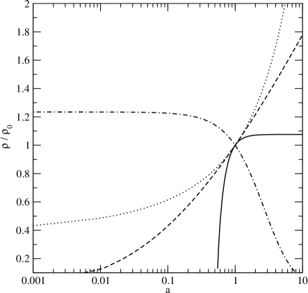
Figure 1: The energy density $\rho$ of the generalized Chaplygin gas (normalized to the present density $\rho_{0}$) as a function of the scale factor $a$ (taken to be $1$ at present). Solid curve is Case 2(a) (early phantom with $\alpha>0$: $A_{s}=1.1,\alpha=0.3$), dashed curve is Case 2(b) (early phantom with $-1<\alpha<0$: $A_{s}=1.2,\alpha=-0.95$), dashed-dot curve is Case 3 (transient GCG, with $A_{s}=0.9,\alpha=-1.5$) and dotted curve is Case 4 (late phantom, with $A_{s}=1.1,\alpha=-1.1$).

Since we are considering the GCG as a dark energy candidate, the expression for the Hubble parameter near the present becomes

$$H^{2} = H_{0}^{2}\biggl{[}\Omega_{m0}(1+z)^{3}+\Omega_{gcg0}[A_{s}$$ (10)

$$+ (1-A_{s})(1+z)^{3(1+\alpha)}]^{1/(1+\alpha)}\biggr{]},$$

where we have assumed a normal dust-like dark matter component with present density parameter $\Omega_{m0}$, and $\Omega_{gcg0}$ is the present value of the density parameter for the GCG component. We have neglected the radiation, which makes a negligible contribution to the total density around the present epoch. We assume a flat universe: $\Omega_{gcg0}=1-\Omega_{m0}$. The equation of state for the GCG fluid is

$$w=-{A_{s}\over{A_{s}+(1-A_{s})(1+z)^{3(1+\alpha)}}}.$$ (11)

Taking $z=0$ in this equation, it is clear that

$$w_{0}=-A_{s},$$ (12)

where $w_{0}$ is the present-day value of $w$ for the Chaplygin gas. Equation (12) gives the physical significance of $A_{s}$.

The behavior of the GCG can vary significantly, depending on the values of $A_{s}$ and $\alpha$. Our aim in this paper is to explore all of these possible behaviours.

We consider first two trivial cases. For $A_{s}=1$, the GCG behaves exactly as a cosmological constant at all times for all values of $\alpha$. For $A_{s}=0$, the GCG behaves as a standard pressureless ($w=0$) dust component for at all times for all values of $\alpha$.

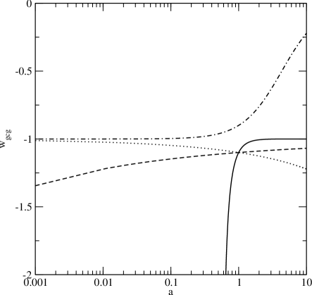
Figure 2: As Fig. 1, for the generalized Chaplygin gas equation of state parameter $w$, as a function of the scale factor $a$.

Now consider the four non-trivial cases corresponding to the pair of choices $A_{s}<1$, $A_{s}>1$, and $\alpha<-1$, $\alpha>-1$.

Case 1) $0<A_{s}<1,\alpha>-1$ (Standard GCG). As previously discussed, in this region the GCG behaves as a pressureless dust component at early times, evolving asymptotically to a de-Sitter regime ($w\rightarrow-1$) at late times. Hence the GCG in this parameter region can act as a unified model for dark energy and dark matter (UDM). This is the standard model of the generalized Chaplygin gas, previously explored in great detail Bento ; gcg1 ; gcg2 ; gcg3 ; gcg4 ; beca3 .

The remaining three cases correspond to “new” versions of the generalized Chaplygin gas.

Case 2) $A_{s}>1$, $\alpha>-1$ (Early Phantom GCG). In this case, the GCG acts as a phantom component with $w<-1$ at all times, but $w$ asymptotically approaches $-1$ at late times. Hence, one has an early phantom behaviour in this region of parameter space. In this case, $\rho_{gcg}=0$ at $1+z_{b}=\left[{A_{s}/(A_{s}-1)}\right]^{1\over{3(1+\alpha)}}$ and then $\rho_{gcg}$ grows to become a constant at late times.

The behavior of this model at early times depends on the value of $\alpha$.

(a) For $\alpha>0$, we have $p_{gcg}\rightarrow-\infty$ when $\rho_{gcg}\rightarrow 0$ at $z=z_{b}$. Hence, there is a pressure singularity at $z=z_{b}$, with $\ddot{a}\rightarrow\infty$, while the scale factor $a$ and the expansion rate $\dot{a}$ remain finite. This is the so-called “sudden singularity” previously discussed by Barrow Barrow . In the classification scheme of Nojiri, Odintsov, and Tsujikawa NOT , this is a Type II singularity. The GCG density $\rho$, the equation of state parameter $w$, and the deceleration parameter $q$ for this case are shown in Figs. 1-3, respectively, as solid curves.

(b) For $0>\alpha>-1$, both $\rho_{gcg}$ and $p_{gcg}$ go to zero at $z=z_{b}$. Although $w\rightarrow-\infty$ at $z=z_{b}$, there is no singularity in this case. Afterwards the GCG behaves as a growing phantom component and then asymptotically approaches the de-Sitter regime ($w\rightarrow-1$) at late times. The values of $\rho$, $w$, and $q$ are shown in this case in Figs. 1-3 as dashed curves.

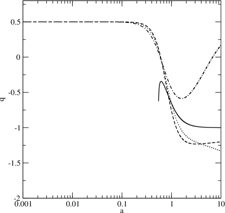
Figure 3: As Fig. 1, for the deceleration parameter $q$ as a function of the scale factor $a$, where we have taken $\Omega_{gcg0}=0.7$ and $\Omega_{m0}=0.3$.

This model has also been examined in some detail in Ref. Lopez . Their main point of emphasis is the interesting fact that this model allows for a phantom equation of state $w<-1$, while avoiding a future singularity. We note further that for $0>\alpha>-1$, this model is free of either past or future singularities, while still allowing for a phantom equation of state.

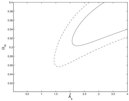
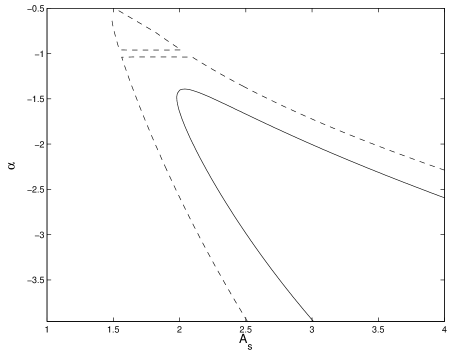
Figure 4: Confidence contours in $\Omega_{m0}-A_{s}$ (left) and $\alpha-A_{s}$ (right) parameter space, marginalizing over $\alpha$ and $\Omega_{m0}$ respectively. Solid and dashed curves are the $68.3\%$ and $95\%$ confidence levels, respectively.

Case 3) $0<A_{s}<1,\alpha<-1$ (Transient GCG). In this case, one has a de-Sitter regime ($w\rightarrow-1$) at early times, while $\rho_{gcg}$ asymptotically approaches pressureless dust ($w\rightarrow 0$) at late times. The GCG density $\rho$, the GCG equation of state parameter $w$, and the deceleration parameter $q$ for this case are shown in Figs. 1-3, respectively, as dot-dash curves.

If the GCG serves as dark energy in this case, the acceleration is a transient phenomenon. Models with transient acceleration are desirable from the point of view of string theory, as the existence of future horizons in an eternally-accelerating universe leads to a well-known problem in constructing the S-matrix in such models Smatrix1 ; Smatrix2 . Hence, a fair amount of effort has gone into constructing models in which the currently-observed acceleration is a transient phenomenon Cline ; Blais ; Sahni2 ; Bilic2 . This case for the GCG represents another such model.

Case 4) $A_{s}>1,\alpha<-1$ (Late Phantom GCG) In this case $\rho_{gcg}$ starts as a constant and then grows and eventually hits a singularity in the future. The equation of state resembles that of a cosmological constant ($w\approx-1$) at early times, and then becomes phantom-like in the future. The future singularity occurs at $1+z_{s}=\left[{A_{s}/{(A_{s}-1)}}\right]^{1\over{3(\alpha+1)}}$. Note that this singularity occurs at a finite value of the scale factor, which is different from the standard phantom scenario in which the scale factor blows up simultaneously with the energy density of the dark energy. This singularity also differs from that in Case 2, as in this case, we have $\rho\rightarrow\infty$ and $p\rightarrow-\infty$ as $z\rightarrow z_{s}$; in the classification scheme of Ref. NOT , this is a Type III singularity. The GCG density $\rho$, the equation of state parameter $w$, and the deceleration parameter $q$ for this case are shown in Figs. 1-3, respectively, as dotted curves.

It is well known that, under very general assumptions, dark energy arising from a scalar field cannot evolve from $w<-1$ to $w>-1$ or vice-versa Vikman ; this has been dubbed the “phantom divide” Hu . The GCG model also displays a phantom divide, characterized by whether or not $A_{s}>1$ or $A_{s}<1$. For all models with $A_{s}<1$, we have $w>-1$ at all times and for all values of $\alpha$, while $A_{s}>1$ gives phantom behavior ($w<-1$) at all times and for all $\alpha$.

Note also that all of the GCG models display asymptotic de Sitter behavior ($w\rightarrow-1$). For $\alpha<-1$, the de Sitter behavior occurs asymptotically in the past, while $\alpha>-1$ gives de Sitter behavior in the asymptotic future. These results are independent of $A_{s}$, which simply determines whether $w$ approaches $-1$ from above or below.

Many other barotropic models have been discussed in the literature, e.g., the Van der Waals model VDW and the wet fluid model water . However, the barotropic model which most closely resembles the GCG models examined here is the model of Ref. Stefancic (see also NOT ), which has the equation of state

$$p=-\rho-B\rho^{\beta}$$ (13)

While this model is qualitatively different from the GCG models, it displays similar behavior in certain limits, particularly with regard to singularities in the evolution. In particular, for $B>0$ and $\beta>1$, the density $\rho$ is an increasing function of the scale factor, so that the second term in equation (13) is dominant at late times. Thus, this model approaches the behavior of our Case 4 model at late times, with a similar singularity NOT ; Stefancic .

III CONSTRAINTS FROM SUPERNOVA DATA

In this section, we will examine constraints on these various versions of the GCG from the supernova Ia data. In deriving these limits, we assume that the GCG acts purely as dark energy, and we take the dark matter to be a separate component.

The observations of supernovae measure essentially the apparent magnitude $m$, which is related to the luminosity distance $d_{L}$ by

$$m(z)={\cal M}+5\log_{10}D_{L}(z)~{},$$ (14)

where

$$D_{L}(z)\equiv{{H_{0}}\over{c}}d_{L}(z)~{},$$ (15)

is the dimensionless luminosity distance and

$$d_{L}(z)=(1+z)d_{M}(z)~{},$$ (16)

with $d_{M}(z)$ being the comoving distance given by

$$d_{M}(z)=c\int_{0}^{z}{{1}\over{H(z^{\prime})}}dz^{\prime}~{}.$$ (17)

Also,

$${\cal M}=M+5\log_{10}\left({{c/H_{0}}\over{1~{}\mbox{Mpc}}}\right)+25~{},$$ (18)

where $M$ is the absolute magnitude.

For our analysis, we consider the data set compiled by Riess et al. riess . The total data set contains the previously published 230 data points from Tonry et al. tonry , along with the 23 points from Barris et al. barris . But Riess et al. have discarded various points where the classification of the supernovae was not certain or the photometry was incomplete, increasing the reliablity of the sample. Ultimately the final set contains 143 points plus the 14 points discovered recently using the Hubble Space Telescope (HST), and this set of 157 points is named the “gold” sample by Riess et al.

The data points in these samples are given in terms of the distance modulus

$$\mu_{\rm obs}(z)\equiv m(z)-M(z)~{}=5\log d_{L}+25,$$ (19)

where $d_{L}$ is measured in Mpc. The $\chi^{2}$ is calculated from

$$\chi^{2}=\sum_{i=1}^{n}\left[{{\mu_{\rm obs}(z_{i})-\mu_{\rm th}(z_{i};H_{0},c_{\alpha})}\over{\sigma_{\mu_{\rm obs}}(z_{i})}}\right]^{2}~{},$$ (20)

where present day Hubble parameter, $H_{0}$, is a nuisance parameter and $c_{\alpha}$ are the model parameters. Marginalizing our likelihood functions over the nuisance parameter $H_{0}$ yields the confidence intervals in the $c_{\alpha}$ parameter space.

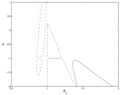
Figure 5: The $68.3\%$ confidence contours in $\alpha-A_{s}$ parameter space for different values of $\Omega_{m0}$. Solid, dashed, dash-dot and dotted lines are for $\Omega_{m0}=0.35,0.30,0.25$, and $0.20$, respectively

.

For our purposes, we have three model parameters, $\Omega_{m0}$, $\alpha$ and $A_{s}$. For our best fit analysis, we vary the parameters in the following ranges: $\Omega_{m0}$ from $0.2$ to $0.4$, $\alpha$ from $-4$ to $4$ and $A_{s}$ from $0$ to $5$. The best fit values for the parameters in this case are: $\Omega_{m0}=0.39$, $\alpha=-3.87$ and $A_{s}=4.99$ together with $\chi^{2}_{min}=172.79$. In Figure 4 we show the confidence contours in the $\Omega_{m0}-A_{s}$, and $\alpha-A_{s}$ parameter space by marginalizing over $\alpha$ and $\Omega_{m0}$ respectively. In both cases, $A_{s}=1$ ($\Lambda$CDM) is rejected at the $95\%$ confidence level, while the data favor $A_{s}>1$ ($w_{0}<-1$). Moreover, from the allowed $\alpha-A_{s}$ space, one can see that a large portion of the allowed region corresponds to Case 4 (late phantom GCG). This is consistent with previous analyses that suggest that the supernova data slightly favor $w<-1$ at present phantom . There is also a small region at the $95\%$ confidence level corresponding to Case 2(b) (early phantom GCG without an initial singularity).

To see how the model parameters depend on $\Omega_{m0}$, we plot in Fig. 5 the $68.3\%$ confidence contours in the $\alpha-A_{s}$ space for different values of $\Omega_{m0}$. This figure shows that the allowed parameters for the GCG depend very sensitively on the assumed value for $\Omega_{m0}$; for this set of choices for $\Omega_{m0}$, any of the four cases is possible. For $\Omega_{m0}=0.2$, the allowed region falls under the Case 1, where GCG behaves as a dust-like dark energy component, asymptotically approaching a cosmological constant. For $\Omega_{m0}=0.25$, the data allow Case 1 as well as Case 3 where the acceleration of the universe is only a transient phenomena as it asymptotically approaches dust-like behavior. For $\Omega_{m0}=0.3$ the data allow Case 2 (both a and b) where the GCG behaves as phantom dark energy at early times but approaches a cosmological constant at late times, as well as Case 4 where the GCG evolves from cosmological-constant-type behaviour to phantom behaviour. For $\Omega_{m0}=0.35$ only Case 4 is allowed. Our results show that $\Omega_{m}\geq 0.3$ is necessary in order to have a phantom-like equation of state. This conclusion is consistent with the recent results of Jassal et al. hari , although they used a different parametrization for the dark energy equation of state.

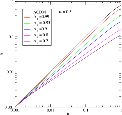
Figure 6: Evolution of the matter density perturbation $\delta$ as a function of the scale factor $a$ (normalized to $a=1$ at the present) for the standard GCG case with $\Omega_{m0}=0.3$.

These results show that the value of $\Omega_{m0}$ is crucial in determining which types of GCG dark energy are consistent with the supernova data. The constraint on $\Omega_{m0}$ in $\Lambda$CDM models from WMAP is $\Omega_{m0}=0.29\pm 0.07$ wmap , which is also consistent with recent results from SDSS observations, while the more recent 2dFGRS analysis gives $\Omega_{m0}=0.237\pm 0.020$ Sanchez . Of course, when $w$ is allowed to vary from $w=-1$, these limits become functions of $w$, but it is clear that the current observational constraints on $\Omega_{m0}$ are insufficient to rule out any of our four possible GCG models using supernova data alone.

IV GROWTH OF LINEAR DENSITY PERTURBATIONS

In this section, we study the growth of density perturbations for the mixture of a matter fluid and a GCG dark energy fluid in the linear regime on subhorizon scales. In performing this calculation, it is necessary to assume a particular clustering behavior for the dark energy. However, this behavior will depend on the physical model that gives rise to the Chaplygin gas equation of state. For example, if the Chaplygin gas is taken to be a perfect fluid satisfying equation (6), then the GCG component will cluster gravitationally with a sound speed given by $c_{s}^{2}=-w\alpha$ Bean . On the other hand, it is also possible to generate minimally-coupled scalar field models with the equation of state given by equation (6) Kamenshchik ; gcg4 (see also Ref. Lopez ). Such models always have $c_{s}=1$ on subhorizon scales and therefore do not cluster on small scales. The evolution of density perturbations for a GCG dark energy component that can cluster gravitationally was examined in Ref. Bean , while the case of a smooth, unclustered GCG dark energy component was examined in Ref. Mul . We take the latter approach here. In this case, the only effect of the GCG evolution is to alter the growth of dark matter perturbations through the effect of the GCG energy density on the expansion of the universe. However, it is important to remember that the results will be very different for the case in which the GCG component is allowed to cluster.

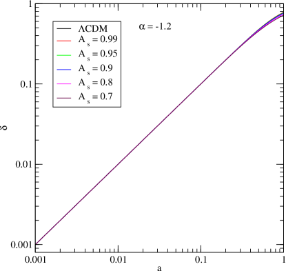
Figure 7: Evolution of the matter density perturbation $\delta$ as a function of the scale factor $a$ (normalized to $a=1$ at the present) for the transient GCG case with $\Omega_{m0}=0.3$.

Assuming the GCG to be a smooth component, the growth equation for the linear matter density perturbation, $\delta$, is given by

$$\delta^{{}^{\prime\prime}}+(2+{{\dot{H}}\over{{H}^{2}}})\delta^{{}^{\prime}}+3c_{1}\delta=0,$$ (21)

where “prime” denotes the derivative with respect to $\ln(a)$, “dot” denotes the derivative with respect to $t$, and $H$ is the Hubble parameter for the background expansion given in equation (10). In equation (21), $\delta$ is the linear matter density contrast, $\delta=\delta\rho_{m}/\rho_{m}$, and $c_{1}$ is given by

$$c_{1}=-{1\over{2}}{\Omega_{m0}\over{\Omega_{m0}+\Omega_{gcg0}[1+A_{s}(a^{3(\alpha+1)}-1)]^{1/(1+\alpha)}}}.$$ (22)

One can easily check that for $A_{s}=1$, the equation reduces to that for the $\Lambda$CDM model. We have integrated equation (21) numerically from $a=10^{-3}$ to $a=1$ (taken to be the present). The initial conditions are choosen such that at $a=10^{-3}$, the standard solution $\delta\sim a$ for Einstein-deSitter universe is reached. Also we have assumed the matter density parameter $\Omega_{m0}=0.3$ throughout. We have studied the solutions for the standard GCG (Case 1), transient GCG (Case 3) and late phantom GCG (Case 4) models.

Figs. 6, 7, and 8 show the behaviour of $\delta$ as a function of the scale factor for these three cases. The standard GCG case has been studied previously by Multamaki et al. Mul , who showed that for parameters slightly deviating from the $\Lambda$CDM universe ($A_{s}=1$), $\delta$ deviates grossly from the standard $\Lambda$CDM result, making this model hard to reconcile with the present observational data. The behaviour of $\delta$ in Fig. 6 agrees with this result.

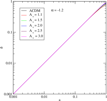
Figure 8: Evolution of the matter density perturbation $\delta$ as a function of the scale factor $a$ (normalized to $a=1$ at the present) for the late phantom GCG case with $\Omega_{m0}=0.3$.

On the other hand, one can see from Figs. 7 and 8 (the transient and late phantom cases respectively), with values of $\alpha$ and $A_{s}$ deviating significantly from the $\Lambda$CDM case, that the behaviour of $\delta$ is practically indistinguishable from the $\Lambda$CDM case. This is an interesting result; it shows that models with GCG dark energy can have quite different equations of state from $\Lambda$CDM at either early or late times, yet still give similar results for the growth of linear density perturbations. The reason for these results is clear from the behavior of $\rho$ for these models (Fig. 1). Both the transient and late phantom GCG models, like the cosmological constant, contribute negligibly to the density of the universe at early times; this density is dominated by the matter component. At low redshift, the GCG in both models begins to dominate the expansion (just as the cosmological constant does in $\Lambda$CDM), with the GCG density decreasing in time (for the transient model) or increasing in time (for the late phantom model). However, these deviations from the behavior of the cosmological constant occur over a very short range in redshift, and by forcing $\Omega_{0}$ for the dark energy to be the same in all three cases, the results for the evolution of density perturbations are almost exactly the same.

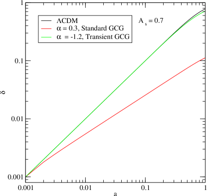
Figure 9: Comparison of the evolution of the matter density perturbation $\delta$ for the transient and standard GCG cases with $\Omega_{m0}=0.3$.

For the standard GCG, in contrast, the dust-like behavior results in a significant contribution to the density of the universe as long as dark matter is the dominant component; if the GCG is assumed not to cluster, the result is a significant decrease in the perturbation growth. This is illustrated more clearly in Fig. 9, where we show $\delta$ as function of the scale factor for both the transient and standard GCG models with the same $A_{s}$ ($A_{s}=0.7$), along with the $\Lambda$CDM model.

Since the observations related to density perturbations are consistent with the $\Lambda$CDM model, our results suggest that, unlike the standard GCG model, both the transient and late phantom GCG models are consistent with the linear growth of density perturbations inferred from observations. We have not shown the results for the early phantom model, but for the case where there is no early singularity, the results are also nearly identical to the $\Lambda$CDM model. Again, we emphasize that these results assume a non-clustering GCG. For the case where the GCG clusters as a perfect fluid, the growth of density perturbations would be quite different.

V CONCLUSIONS

Our exploration of the the full $A_{s}-\alpha$ parameter space for the generalized Chaplygin gas yields three additional models beyond the standard GCG. Although these cannot serve as unified models for dark matter and dark energy, they can have interesting consequences when treated as models for dark energy alone.

The early phantom model (Case 2) has the interesting property of serving as phantom dark energy ($w<-1$) without a late big rip singularity, and for some choices of parameters it is also free of an initial singularity. The transient CGC model (Case 3) provides a mechanism for accelerated behavior at the present, but it asymptotically approaches dust-like behavior at late times (i.e., its time evolution is exactly opposite to the standard GCG model). Thus, it provides a mechanism to allow for present-day acceleration without a future horizon. The late phantom GCG model gives $w<-1$ with $w$ decreasing with time, and it results in a future singularity at a finite value of the scale factor.

All of these models can be made consistent with the type Ia supernovae observations, for an appropriate choice of $\Omega_{m0}$; the question of which models are allowed is extremely sensitive to the value of $\Omega_{m0}$. If the GCG is assumed not to cluster, then all of these models (with the exception of the subset of early phantom models with an initial singularity) are also consistent with the growth of linear density perturbations. Of course, if the GCG is assumed to cluster, then these results will be significantly altered.

Note that all three of our “new” GCG models have a de Sitter phase, and all three models can be tuned arbitrarily close to a cosmological constant at the present, either by pushing the phantom-like behavior arbitrarily far into the past (early phantom model), or by pushing the dust-like or phantom-like behavior arbitrarily far into the future (transient GCG and late phantom model, respectively). These limits may seem uninteresting, as they reduce to the $\Lambda$CDM model over all observable ranges, but the one exception is the transient GCG model. A dust-like phase for this model, even in the far future, eliminates the problem of future horizons. Thus, the transient GCG model can be made arbitrarily similar to the $\Lambda$CDM model but at the same time can resolve the possible conflict between the accelerating universe and string theory.

- (1) V. Sahni, astro-ph/0403324.
- (2) M.S. Turner and M. White, Phys. Rev. D56, 4439 (1997).
- (3) R.R. Caldwell, R. Dave, and P.J. Steinhardt, Phys. Rev. Lett. 80, 1582 (1998).
- (4) A.Y. Kamenshchik, U. Moschella, and V. Pasquier, Phys. Lett. B 511, 265 (2001).
- (5) N. Bilic, G.B. Tupper, and R.D. Viollier, Phys. Lett. B 535, 17 (2002).
- (6) H. Sandvik, M. Tegmark, M. Zaldarriaga, and I. Waga, astro-ph/0212114.
- (7) R. Bean and O. Dore, Phys. Rev. D68, 23515 (2003).
- (8) L.M.G. Beca, P.P. Avelino, J.P.M. de Carvalho and C.J.A.P. Martins, Phys. Rev. D67, 101301 (2003).
- (9) P.P. Avelino, L.M.G. Beca, J.P.M. de Carvalho, C.J.A.P. Martins and E.J. Copeland, Phys. Rev. D69, 041301 (2004).
- (10) M.C. Bento, O. Bertolami, and A.A. Sen, Phys. Rev. D66, 043507 (2002).
- (11) J.D. Barrow, Phys. Lett. B 180, 335 (1986).
- (12) J.D. Barrow, Nucl. Phys. B 310, 743 (1988).
- (13) I.M. Khalatnikov, Phys. Lett. B 563, 123 (2003).
- (14) P.F. Gonzalez-Diaz, Phys. Rev. D68, 021303 (2003).
- (15) L.P. Chimento and R. Lazkoz, astro-ph/0505254.
- (16) L.P. Chimento, Phys. Rev. D69, 123517 (2004).
- (17) M. Bouhmadi-Lopez and J.A.J. Madrid, JCAP 5, 5 (2005).
- (18) M.C. Bento, O. Bertolami and A.A. Sen, Phys. Lett. B575, 172 (2003); Phys. Rev. D67, 063003 (2003); D. Carturan and F. Finelli, Phys. Rev. D68 103501 (2003); Amendola, F. Finelli, C. Burigana and D. Carturan, JCAP 7, 005 (2003).
- (19) J.C. Fabris, S.B.V. Gonçalves and P.E. de Souza, astro-ph/0207430; A. Dev, J.S. Alcaniz and D. Jain, Phys. Rev. D67, 023515 (2003); V. Gorini, A. Kamenshchik and U. Moschella, Phys. Rev. D67, 063509 (2003); M. Makler, S.Q. de Oliveira and I. Waga, Phys. Lett. B555, 1 (2003); J.S. Alcaniz, D. Jain and A. Dev, Phys. Rev. D67, 043514 (2003); M.C. Bento, O. Bertolami, N.M.C Santos and A.A. Sen, Phys. Rev. D71, 063501 (2005).
- (20) P.T. Silva and O. Bertolami, Ap. J. 599, 829 (2003); M.C. Bento, O. Bertolami, and A.A. Sen, Phys. Rev. D70, 083519 (2004).
- (21) O. Bertolami, A.A. Sen, S. Sen and P.T. Silva, Mon. Not. R. Ast. Soc. 353 329 (2004).
- (22) P.P. Avelino, L.M.G. Beca, J.P.M. de Carvalho, C.J.A.P. Martins, and P. Pinto Phys. Rev. D67, 023511 (2003).
- (23) J.D. Barrow, Class. Quant. Grav. 21, L79 (2004).
- (24) S. Nojiri, S.D. Odintsov, and S. Tsujikawa, Phys. Rev. D71, 063004 (2005).
- (25) S. Hellerman, N. Kaloper, and L. Susskind, JHEP 6, 3 (2001).
- (26) W. Fischler, A. Kashani-Poor, R. McNees, and S. Paban, JHEP 0107, 3 (2001).
- (27) J. M. Cline, JHEP 8, 35 (2001).
- (28) D. Blais and D. Polarski, Phys. Rev. D70, 084008 (2004).
- (29) V. Sahni and Y. Shtanov, JCAP 11, 14 (2003).
- (30) N. Bilic, G.B. Tupper, and R.D. Viollier, astro-ph/0503428.
- (31) A. Vikman, Phys. Rev. D71, 023515 (2005).
- (32) W. Hu, Phys. Rev. D71, 047301 (2005).
- (33) S. Capozziello et al., JCAP 4, 5 (2005).
- (34) R. Holman and S. Naidu, astro-ph/0408102.
- (35) H. Stefancic, Phys. Rev. D71, 084024 (2005).
- (36) A. G. Riess et al., Ap. J. 607, 665 (2004).
- (37) J. L. Tonry et al., Ap. J. 594, 1 (2003).
- (38) B. J. Barris et al., Ap. J. 602, 571 (2004).
- (39) U. Alam, V. Sahni, T.D. Saini, and A.A. Starobinsky, Mon. Not. R. Ast. Soc. 354, 275 (2004); U. Alam, V. Sahni, and A.A. Starobinsky, JCAP 6, 8 (2004); T.R. Choudhury and T. Padmanabhan, Astron. and Astrophys. 429, 807 (2005).
- (40) H.K. Jassal, J.S. Bagla and T. Padmanabhan, astro-ph/0506748.
- (41) D. N. Spergel et al., Ap. J. Supp. 148, 175 (2003).
- (42) A.G. Sanchez et al., astro-ph/0507583.
- (43) T. Multamaki, M. Manera and E. Gaztañaga, Phys. Rev. D69, 023004 (2004).