STIS Spectroscopy of Young Star Clusters in “The Antennae” Galaxies (NGC 4038/4039)

Abstract

Long-slit spectra of several dozen young star clusters have been obtained at three positions in the Antennae galaxies with the Space Telescope Imaging Spectrograph (STIS) and its $52{\tt{}^{\prime\prime}}\!\times 0\hbox{$.\!\!^{\prime\prime}$}2$ slit. Based on H$\alpha$ emission-line measurements, the average cluster-to-cluster velocity dispersion in seven different cluster aggregates (“knots”) is $<$10 km s^-1. The fact that this upper limit is similar to the velocity dispersion of gas in the disks of typical spiral galaxies suggests that the triggering mechanism for the formation of young massive compact clusters (“super star clusters”) is unlikely to be high velocity cloud–cloud collisions. On the other hand, models where preexisting giant molecular clouds in the disks of spiral galaxies are triggered into cluster formation are compatible with the observed low velocity dispersions. These conclusions are consistent with those reached by Zhang et al. (2001) based on comparisons between the positions of the clusters and the velocity and density structure of the nearby interstellar medium. We find evidence for systematically lower values of the line ratios [N II]/H$\alpha$ and [S II]/H$\alpha$ in the bright central regions of some of the knots, relative to their outer regions. This suggests that the harder ionizing photons are used up in the regions nearest the clusters, and the diffuse ionized gas farther out is photoionized by ‘leakage’ of the leftover low-energy photons. The low values of the [S II]/H$\alpha$ line ratio, typically [S II]/H$\alpha$ $<$ 0.4, indicates that the emission regions are photoionized rather than shock heated. The absence of evidence for shock-heated gas is an additional indication that high velocity cloud–cloud collisions are not playing a major role in the formation of the young clusters.

1. Introduction

The discovery of young massive star clusters in merging galaxies was one of the important early results from the Hubble Space Telescope (Holtzman et al. 1992; Whitmore et al. 1993). These clusters have all the attributes of young globular clusters, hence providing us with the opportunity to study the formation of these systems in the local universe. Dozens of other galaxies have now been found to harbor similar clusters. Merging galaxies appear to have the largest populations of such “super star clusters,” though similar clusters are also found in smaller numbers in starburst, barred, and even normal spiral galaxies (see Whitmore 2003 for a review). This discovery has acted as a catalyst for the study of star clusters and for the study of star formation in general since it now appears that most stars form in clusters (e.g., Lada & Lada 2003; Fall et al. 2005).

What triggers the formation of these young, compact, massive clusters? One possibility is that high-velocity collisions of the gaseous components in interacting galaxies result in the formation of large-scale shock fronts that trigger gravitational collapse and the subsequent formation of stars and clusters (e.g., Gunn 1980; Schweizer 1987; Kang et al. 1990; Olson & Kwan 1990a, 1990b; Noguchi 1991; Kumai et al. 1993a, 1993b). Specifically, Kumai et al. 1993a suggest that chaotic cloud–cloud collisions with velocities $\geq$ 50 – 100 km s^-1 may result in the formation of young globular clusters due to local shock compression in the Magellanic Clouds. A more recent model by Bekki et al. (2004) suggests that velocities in the range 10 – 50 km s^-1 are optimal for making clusters. Recent numerical, smooth-particle-hydrodynamic simulations of NGC 4676 (“The Mice”) by Barnes (2004) have been successful in reproducing the extended nature of star formation in this interacting galaxy pair with a shock-induced star-formation law. However, it is important to note that much of the extended star formation in this model originates in relatively low-velocity shocks due to convergent flows, rather than in high-velocity shocks created by interpenetrating collisions of galactic disks. Some observational support for cluster formation being triggered by high-velocity collisions comes from Wilson et al. (2000), who find that the strongest CO and IR source in the Antennae galaxies coincides with a knot in the “Overlap Region”, where two giant molecular clouds appear to be colliding with differential velocities of 50 – 100 km s^-1.

There is, however, direct evidence against high-speed cloud collisions being the dominant triggering mechanism for the formation of star clusters in the Antennae galaxies. Zhang et al. (2001) made detailed comparisons between the positions of star clusters in the Antennae and the stellar and interstellar contents of these galaxies, based on observations over a wide range of wavelengths. They found little or no correlation between the positions of young clusters (very near their birthplaces) and the velocity structure of the surrounding interstellar medium, as measured by gradients and dispersions in the HI and H$\alpha$ channel maps at various distances from the clusters, as would be expected if cloud motions triggered the formation of the clusters (see Figures 15, 16, and 17 of Zhang et al. 2001). In contrast, Zhang et al. found a strong correlation between the positions of the young clusters and several other properties, including gaseous emission from young stars and the density structure of the surrounding interstellar medium as measured by the HI and CO intensity maps. The implications of these results for the formation of the clusters are discussed further by Fall (2004).

In the present paper we measure the velocities of several dozen young clusters in the Antennae by using the high spatial resolution made possible by the Hubble Space Telescope (HST ), and from these compute the corresponding velocity dispersion. While previous ground-based studies (e.g., Burbidge & Burbidge 1966; Rubin et al. 1970; Amram et al. 1992) mapped out the velocities of various “knots” in The Antennae (e.g., labeled A through T by Rubin et al.), the Hubble observations by Whitmore & Schweizer (1995) revealed that each of these “knots” consists of roughly a dozen or more individual star clusters. Long-slit spectroscopic observations with the Space Telescope Imaging Spectrograph (STIS) can provide a direct measurement of the velocity dispersion between clusters within such knots. If clusters formed in high-speed cloud collisions, we might expect the resulting velocities of the clusters, and hence their dispersion, to be large. The main caveat here concerns the possibility that some of the kinetic energy of cloud motions is dissipated and radiated away during the collisions and hence is not fully reflected in the velocity dispersion among the clusters. If we neglect this dissipation for the moment, the observed velocity dispersion among the clusters should reflect the velocity dispersion of the clouds from which they formed. This is the test we perform here, as a complement to the one reported by Zhang et al. (2001).

Throughout the present paper we adopt a Hubble Constant of $H_{0}=75$ km s^-1 Mpc^-1, which for a heliocentric systemic velocity of $cz_{\odot}=1630$ km s^-1 (corresponding to 1440 km s^-1 relative to the Local Group) places NGC 4038/4039 at a distance of 19.2 Mpc. At this distance, the projected scale is $1{\tt{}^{\prime\prime}}=93$ pc, and the corresponding distance modulus is 31.41 mag. We note that Saviane et al. (2004) determine a distance of only $13.8\pm 1.7$ Mpc for The Antennae, based on the tip of the red giant branch observed in the southern tidal-tail population. This distance would imply a peculiar velocity of $\sim$400 km s^-1, which would be quite high for a field galaxy in a loose group such as NGC 4038/4039. We prefer to use the original redshift distance for this paper, pending a more definitive measurement of the photometric distance.

2. Observations and Reductions

Long-slit spectra of the Antennae galaxies were obtained with STIS during the period from 2000 April to 2001 March, as part of Proposal GO-8170. A variety of observations were made, including long-slit H$\alpha$ observations (G750M grating), both long-slit and slitless observations in the UV (G140L grating), and slitless observations in the blue (G430M grating). Most results in the current paper are based on the H$\alpha$ observations. More detailed results from observations with the G140L and G430M gratings will be reported in a future paper. Chandar et al. (2005) also use the G140L spectra in their study of the ages of clusters in 27 star-forming galaxies. Their spectroscopically determined ages are in good agreement with the photometrically determined ages reported in the present paper.

Table 1 presents a variety of measured and derived parameters for the cluster candidates discussed in this paper. These include the cluster ID number (from Whitmore & Zhang 2002), a quality index based on how well the H$\alpha$ and I-band images correspond, absolute magnitude ($M_{V}$), age estimate (from Whitmore & Zhang 2002), equivalent width of H$\alpha$, velocity, line width, relative H$\alpha$ flux, and [NII]/H$\alpha$ and [SII]/H$\alpha$ line strength ratios. As discussed below, in cases when the emission appears to be diffuse (e.g., the quality = 3 candidates), we include the nearest cluster in the table in order to obtain information about the physical characteristics within the knot (e.g., the mean age of nearby clusters).

A $52{\tt{}^{\prime\prime}}\!\times 0\hbox{$.\!\!^{\prime\prime}$}2$ slit was used with the G750M grating to cover the spectral region of $\lambda\lambda$6500 – 7050 Å, hence including the [NII] $\lambda\lambda$6548, 6583, H$\alpha$, and [SII] $\lambda\lambda$6716, 6731 lines. The scale was 0.05^′′ pixel^-1, the reciprocal spectral dispersion 0.56 Å pixel^-1, and the spectral resolution for a nominal point source $\sim$0.9 Å (FWHM).

For the observations, three slit positions were selected to include as many young clusters as possible, as shown in Figure 1. We note the curious linear alignments of clusters utilized in visits 6 and 7. It is unclear whether these alignments are due to chance, the edges of occulting dust clouds (which are often found to be filamentary and roughly linear), or perhaps shock fronts formed at the intersection of the two colliding galactic disks. In any case, the fortuitous alignments allowed us to include one to two dozen clusters along each of the three slit positions.

Figures 2a–c show the three long-slit spectra. Note that the continuum can only be seen for the brightest knots. Figure 3 shows an interesting, peculiar steep-gradient feature in the spectrum of Knot B (Visit 6). This feature is visible in both the H$\alpha$ and [NII] lines. The fact that the feature appears tilted indicates that it stems from a spatially directed, rather than spherically symmetric outflow. There is no obvious corresponding feature visible in the H$\alpha$ and broad-band images.

The three exact positions of the slit were determined post facto by comparing the H$\alpha$ flux profiles measured along the slit with linear brightness extractions from our H$\alpha$ image (Whitmore et al. 1999) taken with the Wide-Field Planetary Camera 2 (WFPC2). Figures 4a–c compare the imaging and spectral profiles for each visit. Using this method we were able to determine positions of the slit with an accuracy of about $0\hbox{$.\!\!^{\prime\prime}$}1$, good enough to deduce which specific objects fell on the slit (Table 1). Note that the slightly poorer spatial resolution of the WFPC2 H$\alpha$ image relative to the STIS data makes some of the objects appear less prominent in Figs. 4a–c. Figures 5a–c show the slit positions superposed on both H$\alpha$ and $I$-band WFPC2 images.

Note that not all of the peaks in the H$\alpha$ profiles are due to clusters; some are due to shells and other diffuse emission between the clusters. In particular, the fraction of H$\alpha$ peaks associated with diffuse emission rather than clusters was higher in Knot T, presumably because the clusters there tend to be slightly older and have had more time to expel their gas. We include a “quality” index to represent the degree of certainty of our cluster assignments in column 4 of Table 1. This is also why we refer to “candidate” clusters rather than one-to-one matches. In cases when the emission appears to be diffuse, we include information about the nearest cluster in the table in order to obtain information about the physical characteristics within the knot (e.g., the mean age of the nearby clusters). Hence it should be kept in mind that for the quality = 3 objects, the various properties (e.g., the equivalent widths) listed in Table 1 are not for the same region that we have sampled from our slit spectrum.

Table 2 summarizes the mean properties of the seven primary knots covered by our slit positions. The ages of the clusters within these knots were derived using the technique described in Whitmore & Zhang (2002), but using the Bruzual & Charlot (2003) models rather than their 2000 models. Note the correlation between the quality index and the age of the clusters. As expected, the younger clusters show a better correspondense between their H$\alpha$ and continuum morphologies (i.e., lower quality index), since the gas has not had much time to be spatially displaced from the clusters. We also note the extreme youth ($\sim$2 Myr) of some of these clusters, befitting their large equivalent widths.

The limited pointing accuracy, and difficulties in determining optimal positions for the slit, resulted in typical deviations of a few tenths of an arcsecond from some desired positions. This caused us to miss some of the brightest clusters (e.g., we skirted the edge of Knot B in Visit 7). However, with so many clusters in each knot, missing one cluster generally meant that we picked up another cluster somewhere else along the slit. Hence the total number of clusters was roughly the same as originally planned.

The original data were recalibrated using CALSTIS with the most recent reference files. Hot pixels were removed with an IDL routine that replaces deviant pixels by the median of the adjacent pixels. Line strengths, line widths (FWHM of a Gaussian profile), and velocities were measured using the SPECFIT program within STSDAS, with results given in Table 1. The simplex algorithm was used to interactively fit Gaussians to all five emission lines simultaneously. Measurements were made both in and between the clusters whenever the line flux warranted it. Extraction regions ranged from 3 pixels ($0\hbox{$.\!\!^{\prime\prime}$}15$) for bright regions to 24 pixels ($1\hbox{$.\!\!^{\prime\prime}$}2$) where the line flux was weak. Values for the velocity were taken from the H$\alpha$ peak alone since the weaker lines are absent for faint sources. Figures 6a–c present the relative H$\alpha$ flux (solid lines), velocity $cz$, H$\alpha$ line width, [NII]/H$\alpha$ line ratio, and [SII]/H$\alpha$ line ratio for the three visits.

A potential complication is the fact that the clusters are partially resolved within the $0\hbox{$.\!\!^{\prime\prime}$}2$-wide slit. This means that part of the measured velocity is due to the off-center position of clusters within the slit. Because of this, the velocity dispersions reported below represent upper limits. In principle it should be possible to correct for this effect by convolving the H$\alpha$ image with the slit transmission function. However, a rough empirical check indicated that this effect was barely discernible, whence no corrections were applied for the present paper. The affect is very small, in any case, as demonstrated by the small RMS deviations of radial velocities along the slit, as we will discuss later in the paper.

This complication is more serious for our G140L and G430M spectra, most of which were taken with a $0\hbox{$.\!\!^{\prime\prime}$}5$ rather than a $0\hbox{$.\!\!^{\prime\prime}$}2$ slit. We attempted to circumvent this problem by measuring wavelengths for the Milky Way components of strong interstellar lines (e.g., C II $\lambda 1335$ and Si II $\lambda 1260$) in order to determine a wavelength zeropoint for the spectra. Due to the radial velocity of the Antennae, ISM lines arising in the Antennae are redshifted relative to the same lines arising in the Milky Way; hence, in principle we should be able to see both the Galactic and Antennae components. Figures 21 and 23 in Whitmore et al. (1999) show that this is indeed the case for Knots S and K, that are dominated by two of the brightest clusters in the Antennae. Unfortunately, the S/N and spatial resolution of the current spectra were too low for this method to be applied here successfully.

A comparison of the newly determined velocities with published values for Knots B, C, D, E, F, and T shows a relatively large range in absolute differences, especially against the early low-dispersion work by Burbidge & Burbidge (1966; mean difference of +48 km s^-1, with a dispersion of 62 km s^-1). The agreement is much better for velocities measured by Rubin et al. (1970; mean difference of +10 km s^-1, dispersion of 34 km s^-1) and Amram et al. (1992; mean difference of +15 km s^-1, dispersion of 18 km s^-1). A comparison with the HI velocities from Hibbard et al. (2001) is problematic, due to the large mismatch in spatial resolution (i.e., $\sim$$0\hbox{$.\!\!^{\prime\prime}$}1$ for the HST data and $\sim$10^′′ for the HI data), but a rough estimate yields a mean difference of –3 km s^-1 and a dispersion of 48 km s^-1. The differences are in the sense that the earlier papers found larger velocities.

3. Results

3.1. Cluster-to-Cluster H$\alpha$ Velocity Dispersions

A primary goal of this project is to determine whether high cloud–cloud velocity dispersions are the triggering mechanism for the formation of super star clusters, as predicted by some models (e.g., Kumai et al. 1993a, Bekki et al. 2004).

Assuming the gas clouds were already present before the collision (i.e., GMCs), one might expect that the resulting dispersion after the encounter would be comparable to the original velocity difference between the two colliding systems. For example, if portions of two colliding galaxies encountered each other with relative velocities of 100 km s^-1, one might expect a cluster forming from the collision of a high-mass cloud of velocity 100 km s^-1 with a low-mass cloud of velocity 0 km s^-1 to have a resulting velocity near 100 km s^-1. On the other hand, if instead the high-mass cloud had a velocity of 0 km s^-1, the resulting cluster would have a velocity near 0 km s^-1. In practice the situation is likely to be much more complicated, with dissipation, multiple collisions, and turbulence all playing important roles. Hence, we would expect the observed cluster-to-cluster velocity dispersion to be somewhat lower than the original cloud–cloud velocity dispersion.

A cursory glance at Figures 6a–c reveals immediately that the velocity fields along the slit positions are relatively quiescent, with velocity dispersions $\sim$10 km s^-1 rather than the $\sim$100 km s^-1 difference in the orbital velocities of the two colliding galaxies. We note that these low observed cluster-to-cluster velocity dispersions are similar to those found for gas, young stars, and young clusters in normal spiral disks (Mihalas & Binney 1981). While it is conceivable that the inelasticity of cloud–cloud collisions discussed in the previous paragraph might reduce the observed velocity dispersion of a system of clusters formed by high velocity encounters to this degree, it seems too coincidental that the resulting velocity dispersion would essentially match the value found in normal disks.

The low cluster-to-cluster velocity dispersions we have observed are more compatible with models where the GMCs in the disks of the colliding spiral galaxies are the seeds that form the young massive clusters (e.g., Jog & Solomon 1992; Elmegreen & Efremov 1997), rather than with models where large cloud–cloud velocity dispersions are required (e.g., Kumai et al. 1993a, Bekki et al. 2004). In the former case the cluster-to-cluster velocity dispersion would be roughly the same as the original cloud–cloud velocity dispersion, i.e., similar to the velocity dispersion of the gas in a spiral disk.

These conclusions are consistent with those reached by Zhang et al. (2001), as discussed in the introduction, who found little or no correlation between HI and H$\alpha$ velocity dispersions and the presence of young clusters in The Antennae. This interpretation is also supported by the fact that young massive clusters are distributed throughout The Antennae rather than being located only in the “Overlap Region,” where high-speed collisions are most likely to occur. Similarly, young massive clusters are also found in quiescent environments such as normal spiral galaxies (Larsen & Richtler 2000), albeit in smaller numbers.

We have measured the cluster-to-cluster velocity dispersion by selecting knots with three or more measured clusters (i.e., Knots B, C, D, E, F, T, and T2), as listed in Table 2. In several cases there are velocity gradients across the knots which are part of the large-scale velocity field (e.g., Knot F in Visit 7). We corrected for such gradients by fitting a line to the velocities as a function of position in the knot and computing the RMS of the velocity residuals. The clusters in a typical knot extend $\sim$5^′′ along the slit, corresponding to $\sim$500 pc (see Table 2 for individual knots).

A potential complication for this procedure is that in some cases (primarily Knot C) the velocity field is dominated by a super bubble surrounding the knot, with the central part of the knot appearing blue-shifted by $\sim$50 km s^-1 with respect to its surroundings. This effect can be seen most clearly in Figure 2 of Amram et al. (1992), where the velocity contours around Knots B and C appear to be concentric rings.

Table 2 shows that the cluster-to-cluster velocity dispersions measured from the ionized gas are low in all knots. Averaging over all seven knots yields a mean value for the cluster-to-cluster velocity dispersion of 9.6 km s^-1. Excluding Knot C from the average, because of the potential bias introduced by the super bubble, yields a negligible difference (i.e., an average value of 9.5 km s^-1). As discussed in §2, the measured velocity dispersions represent upper limits, since no correction has been made for the position of each cluster within the slit.

Globular cluster systems in galaxies show much larger velocity dispersions than gas in disks. If the young massive clusters in The Antennae are to form a cluster system with kinematics similar to the kinematics of globular clusters in typical early-type galaxies, they need to decouple from the gaseous kinematics. This presumably happens later in the merger, when the process of violent relaxation peaks. The relatively ordered rotational velocity field observed in The Antennae by Burbidge & Burbidge (1966), Rubin et al. (1970; esp. §IV), and Amram et al. (1992, esp. Fig. 2) argues that the original disks are still relatively intact, and most of the violent relaxation lies still ahead.

The low cluster-to-cluster velocity dispersions we have observed in the Antennae beg the question of whether the multiple clusters in a given “knot” are gravitationally bound to each other, and hence may merge together to form more massive clusters, as advocated by various authors (e.g., Kroupa 1998, Elmegreen et al. 2000, Fellhauer et al. 2005, Bekki et al. 2004). Using the virial theorem, and typical values of M_knot = 4 $\times$ 10⁶ M_⊙ (each knot typically including $\approx$ 25 individual clusters with mass greater than 10⁴ M_⊙) and R_knot = 120 pc for our five best defined knots (i.e., B, C, D, F, T), we estimate that the binding velocity is $\approx$ 7 km s^-1 (ranging from 5 to 10 km s^-1 for the five knots). While this is roughly at the limit where we can make reliable measurements based on the current observations, we note that our observed upper limit for the cluster-to-cluster velocity dispersion is only slightly larger than this estimated binding velocity, hence the merging cluster scenario may be viable, at least in part, and deserves further study.

However, it is important to note that the resulting structure that forms from the coalescence of all of the clusters in a knot would have a radius similar to the original radius of the knot (i.e., $\approx$ 100 pc), and hence would look more like a dwarf galaxy than a globular cluster. It may still be possible to form structures with radii similar to globular clusters (or the slightly larger “faint fuzzy” clusters observed by Brodie & Larsen 2002) if only two or three clusters within $\approx$ 10 pc of each other merge.

It is also interesting to compare the cluster-to-cluster H$\alpha$ velocity dispersions with the HI velocity dispersions measured by Hibbard et al. (2001) and here listed in the last column of Table 2. The measured HI velocity dispersions range from 15 to 30 km s^-1, typically a factor of two higher than the cluster-to-cluster velocity dispersions. This apparent discrepancy is almost certainly due to the poor spatial resolution of the HI maps ($\sim$10^′′). For example, Knots T and F both show relatively large H$\alpha$ velocity gradients that we remove when computing the cluster-to-cluster velocity dispersion, but that remain included in the high measured HI velocity dispersions. If the gradient is not removed the cluster-to-cluster H$\alpha$ velocity dispersions are 28.9 km s^-1 for Knot T and 31.2 km s^-1 for Knot F; very similar to the values for the HI velocity dispersions.

3.2. H$\alpha$ Line Widths

In principle, it should be possible to learn about the kinematics of the outflows around clusters and knots from the line-width information. Unfortunately, the ability to decipher this information is compromised by the fact that the $0\hbox{$.\!\!^{\prime\prime}$}2$ width of the slit is comparable to the width of the STIS point spread function. Hence, an apparent increase in the line width may be due to the presence of diffuse line emission covering the slit more uniformly than a point source would, rather than being indicative of a kinematic signature.

According to Table 13.40 of the STIS Instrument Handbook, the instrumental FWHM of spectral lines is $\sim$40 km s^-1 for point sources and $\sim$105 km s^-1 for very extended sources. Note that the latter number is very approximate and likely to be a slight underestimate, since it assumes a simple rectangular profile without taking into account the instrumental wings beyond the edges of the slit. In addition, the program used for analysis (IRAF task SPECFIT) fits a Gaussian profile rather than a rectangular profile. Hence, direct comparisons with predictions of the line profile for a uniform diffuse source are problematic.

The measured line widths in the high S/N knots range from about 70 to 120 km s^-1 (Figure 6). Hence, it seems likely that the observed spread is due to the presence of a range of objects from partially resolved compact star clusters to extended emission from gas that has been expelled from the clusters and fills the slit nearly uniformly. Because of the fact that the upper limit of the measured line profiles is comparable to what is predicted for diffuse emission, we conclude that in general there is no evidence for outflows with velocities greater than $\approx$ 100 km s^-1.

Two possible exceptions occur in clusters #7 and #14 (Visit 6), both with large apparent velocity widths ($>$150 km s^-1) and good signal-to-noise ratios of H$\alpha$ (i.e., relative H$\alpha$ flux $>$50 in Table 1). Cluster #14 lies in the brightest part of Knot B. Figure 3 shows a peculiar steep-gradient feature in its spectrum, with a peak-to-peak velocity amplitude of 150 km s^-1. This feature is probably responsible for the high velocity width measured in Cluster #14. The direct H$\alpha$ image (Fig. 5b) shows—to one side of this cluster—the presence of a large shell-like structure that may be associated with the spectral feature. The other high-velocity-width feature is seen in Cluster #7 (Visit 6), midway between Knots C and D (Figs. 2b and 5b). Careful inspection of Figure 2b and 6b suggests that the superposition of diffuse gas from Knots C and D, plus a discrete cluster at a slightly lower velocity, may in this case be the explanation for the high apparent velocity width.

Knot T represents a case where diffuse emission probably plays the dominant role in determining the line width. The correspondence between the H$\alpha$ and $I$-band images is particularly bad in this knot (i.e., “quality” rating of 3 for seven out of eight objects in Table 1), probably because the clusters are older (mean age $\sim$6 Myr). Hence the gas has had more time to escape, resulting in diffuse emission which fills the slit more uniformly than a point source, resulting in higher apparent line widths ($\sim$110 km s^-1).

This interpretation is supported by the fact that the H$\alpha$ and [N II] lines across Knot T (Fig. 2a) show a series of wiggles, with peak-to-peak velocity amplitudes of $\sim$60 km s^-1 (see Fig. 6a, around position 500). Note from Fig. 6a that the line widths are $\sim$110 km s^-1, consistent with diffuse emission filling the slit. These wiggles are relatively rare, and are largely responsible for Knot T having one of the largest measured cluster-to-cluster velocity dispersions (14 km s^-1, see Table 2). Whitmore et al. (1999) inferred similarly high values for the gas outflow velocities around Knots S and K based on the sizes of the bubbles and age estimates. Hence, it appears likely that the observed line wiggles are related to the outflow velocities produced by individual cluster winds around some of the older clusters. In such cases, the stellar cluster-to-cluster velocity dispersions are likely to be smaller than the gaseous velocity dispersion. Even so, the gaseous velocity dispersion for Knot T is only 14 km s^-1.

The interpretation is simpler for knots that have low apparent velocity widths, indicative of cases where the emission is coming from compact regions around relatively point-like clusters rather than from diffuse emission that fills the slit and artificially broadens the observed line width. We can infer that the clusters are particularly young in these cases and have therefore not had time to blow sizable bubbles of diffuse emission that fills the slit. Probably the best example of this is Knot D (Fig. 6b), with line widths around 80 km s^-1 and a relatively good correspondence between the H$\alpha$ and $I$ images (i.e., no clear evidence for the presence of shell-like structures such as those seen in Knots B and C). We also note that this is one of the younger knots, with a mean age for the clusters of $\sim$2.5 Myr according to Table 2. In addition, Fig. 5c shows that the spectrograph slit was positioned near the center of this knot, whence most of the emission is coming from the bright clusters rather than from the diffuse emission in the area. Similarly, Knot F has line widths around 80 km s^-1, and a mean age of the clusters of $\sim$1.4 Myr.

We conclude that the apparent velocities derived from line widths are primarily useful for providing information about whether the emission is relatively point-like or diffuse, rather than providing information about the actual outflow velocities in the gas. We note that this provides a second-order method for estimating cluster ages, since the knots with low apparent line widths (i.e., more point-like emission) tend to contain the youngest clusters.

3.3. Line-Strength Ratios

Figures 6a–c show how the [N II]/H$\alpha$ and [S II]/H$\alpha$ line ratios change along each of the three long-slit positions. In each case, what is plotted is the sum of two lines ($\lambda$6584 + $\lambda$6548 for [N II], $\lambda$6716 + $\lambda$6731 for [S II]) relative to H$\alpha$.

Several different effects are visible in these figures. Overall, the mean [N II]/H$\alpha$ ratio observed is $\sim$0.4, and the mean [S II]/H$\alpha$ ratio is $\sim$0.2. Faint knots, such as seen in the right half of Fig. 6a (Visit 2 - Region T2), show a large dispersion due to observational uncertainties (i.e., clusters with relative H$\alpha$ flux $<$ 50 in Table 1 have observational uncertainties $\sim$ 0.25), but are consistent with these mean values. Secondly, there is evidence for systematically lower values of the line ratios in a few of the knots where the slit crosses emission of especially high surface brightness. This results in the U-shaped line ratio patterns in Fig. 6b, Knots B, C, and D. This anti-correlation has been seen before in studies of extragalactic H II regions and diffuse ionized gas (DIG) (Hoopes et al. 1999; Greenawalt et al. 1998). Assuming that the DIG is photoionized by ‘leakage’ of leftover ionizing photons from star-forming regions, the harder ionizing photons must be depleted locally causing a higher mean ionization in the central parts of H II regions (and thus lower [S II]/H$\alpha$ and [N II]/H$\alpha$ ratios) than in the surrounding, lower-surface-brightness diffuse gas.

The [S II]/H$\alpha$ ratio is of interest because it has long been used as a discriminant for shock-heated versus photoionized gas (see Blair & Long 1997; Gordon et al. 1998; and references therein). Usually, a criterion with [S II]/H$\alpha$ = 0.4 as the nominal threshold is used. Shock-heated nebulae tend to exhibit higher values of this ratio (often considerably higher), while photoionized nebulae show lower values (often below 0.2). We see no bright, discrete nebulae sampled by the long slits here that exhibit elevated [S II]/H$\alpha$ ratios that would be indicative of shock heating. Hence, no supernova remnants containing bright radiative shocks such as seen in the Cygnus Loop in our Galaxy (e.g., Fesen et al. 1985) have been detected serendipitously in these observations.

The absence of obvious kinematic or line ratio evidence for shock-heated gas in the vicinity of the young clusters provides an additional indication that high velocity cloud–cloud collisions are not playing a major role in the formation of the young clusters. We should note, however, that our observations do not rule out the presence of low–velocity shocks that heat and compress the molecular clouds, since cooling takes place primarily through molecular lines in the IR in this case, rather than leaving a signature in the [S II]/H$\alpha$ ratio.

4. Summary

The Space Telescope Imaging Spectrograph (STIS) aboard the Hubble Space Telescope has been used to obtain long-slit, high-spatial-resolution spectra at three positions in the Antennae galaxies. Observations were made in three spectral regions: the far UV (1150 – 1720 Å), the UV–Blue (3800 – 4100 Å), and the Red including the H$\alpha$, [NII], and [SII] emission lines. This paper focuses on the latter emission lines. The primary results are as follows.

1. The average cluster-to-cluster H$\alpha$ velocity dispersion in seven cluster aggregates (“knots”) is $<$10 km s^-1 and, therefore, similar to the velocity dispersion of the gas and young stars in the disks of spiral galaxies.

2. This low cluster-to-cluster velocity dispersion does not favor models that require high-velocity cloud–cloud collisions to trigger cluster formation (e.g., Olson & Kwan 1990a, b; Kumai et al. 1993a, Bekki et al. 2004). On the other hand, models where giant molecular clouds (GMCs) already present in galactic disks act as the seeds from which young star clusters form are compatible with the observed low velocity dispersions. This also supports earlier findings (Zhang et al. 2001) that there is little or no correlation between HI and H$\alpha$ velocity dispersions and the presence of young clusters in The Antennae.

3. The line ratios of [N II]/H$\alpha$ and [S II]/H$\alpha$ across knots often show U-shaped patterns, with low values where the spectrograph slit crosses the brightest clusters. This suggests that the harder ionizing photons are depleted in regions nearest the clusters, and the diffuse ionized gas farther out is photoionized by ‘leakage’ of the leftover low-energy photons.

4. The observed low values of the [S II]/H$\alpha$ line ratio (typically $\lesssim$0.4) indicate that the HII regions associated with knots and clusters are photoionized rather than shock heated. No supernova remnants containing bright radiative shocks have been detected serendipitously by our observations. The absence of evidence for shock-heated gas in the vicinity of the young clusters provides an additional indication that high velocity cloud–cloud collisions are not playing a major role in the formation of the young clusters.

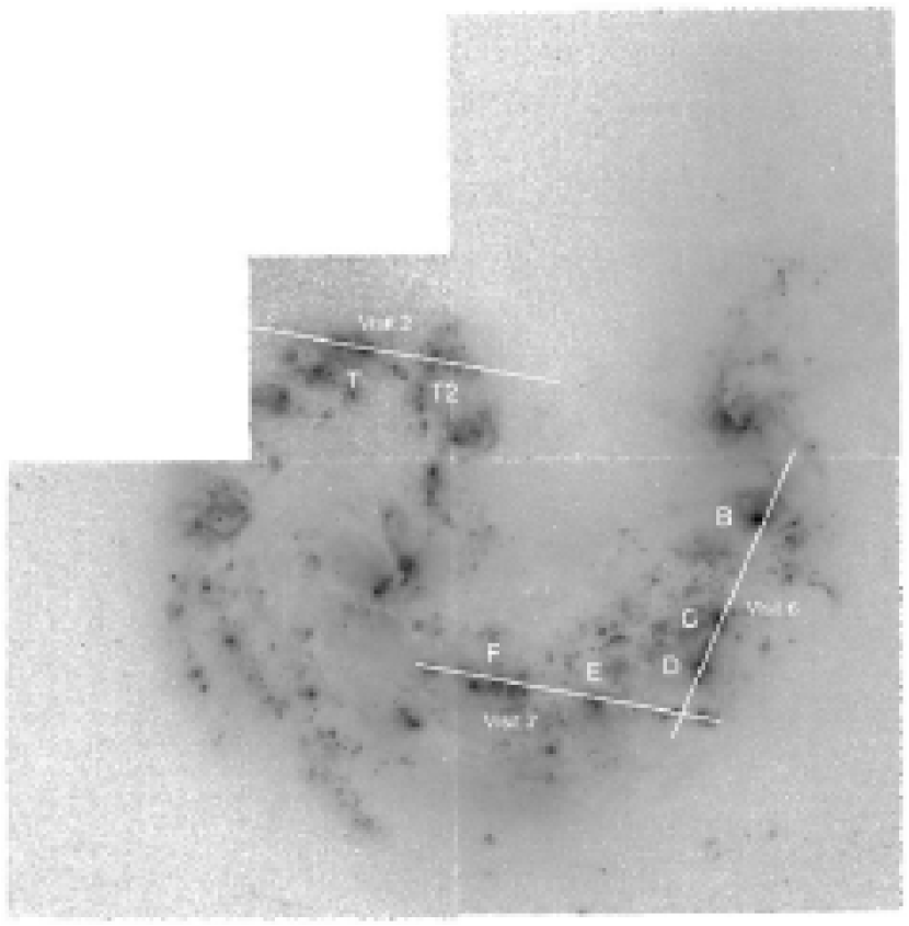
Figure 1.— Slit positions superposed on the $I$-band HST  image of The Antennae for the three visits using the H$\alpha$ grating. Capital letters identify knots named by Rubin et al. (1970).

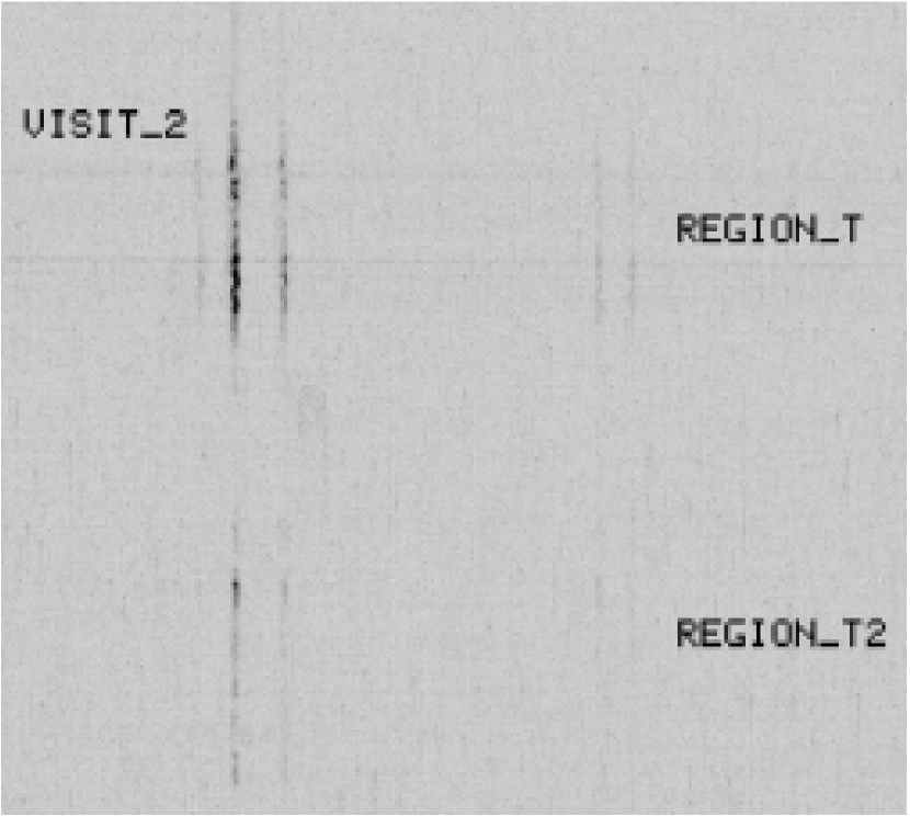
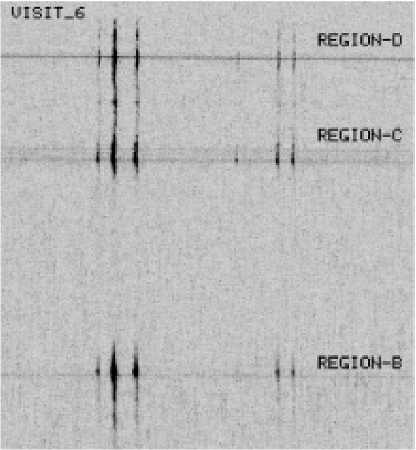
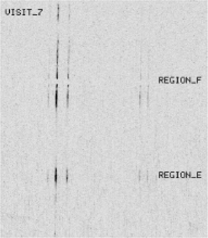
Figure 2.— (2a) Spectrum obtained with the H$\alpha$ grating during Visit 2. Wavelength increases toward the right; the spatial dimension is up and down. The lines are (left to right): [NII] $\lambda$6548, H$\alpha$, [NII] $\lambda$6583, and [SII] $\lambda\lambda$6716, 6731. (2b) Spectrum obtained with the H$\alpha$ grating during Visit 6. The line visible in Knots C and D blueward of the [SII] doublet is He I $\lambda$6678. (2c) Spectrum obtained with the H$\alpha$ grating during Visit 7.

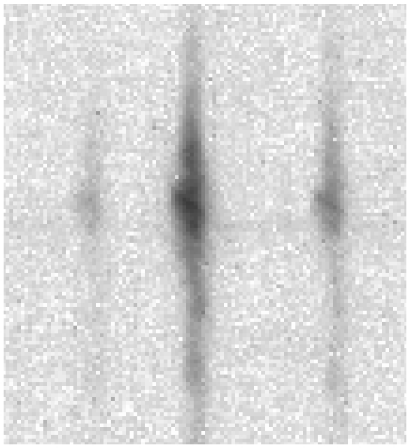
Figure 3.— Blowup of spectrum of Knot B, including an unusual steep-gradient feature.

Figure 4.— (4a) Comparison of H$\alpha$ profile along the slit during Visit 2 with an extraction from a simulated slit on the WFPC2 H$\alpha$ image. ID numbers refer to objects in Table 1 and Figure 5a. (4b) Comparison of H$\alpha$ profile along the slit during Visit 6 with an extraction from a simulated slit on the WFPC2 H$\alpha$ image. ID numbers refer to objects in Table 1 and Figure 5b. (4c) Comparison of H$\alpha$ profile along the slit during Visit 7 with an extraction from a simulated slit on the WFPC2 H$\alpha$ image. ID numbers refer to objects in Table 1 and Figure 5c.

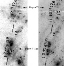
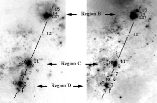
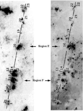
Figure 5.— (5a) Slit position and candidate clusters for Visit 2 superposed on the H$\alpha$ image. Note that the numbers refer to the candidate clusters defined in Table 1, and Figure 4. (5b) Slit position and candidate clusters for Visit 2 superposed on the $I$ image. (5c) Slit position and candidate clusters for Visit 6 superposed on the H$\alpha$ image (5d) Slit position and candidate clusters for Visit 6 superposed on the $I$ image (5e) Slit position and candidate clusters for Visit 7 superposed on the H$\alpha$ image (5f) Slit position and candidate clusters for Visit 7 superposed on the $I$ image.

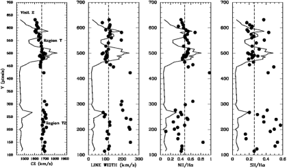
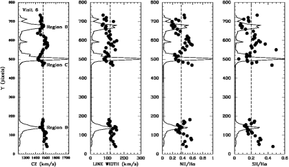
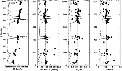
Figure 6.— (6a) Relative H$\alpha$ flux (solid lines), velocity $cz$, H$\alpha$ line width, and [NII]/H$\alpha$ and [SII]/H$\alpha$ line ratios for Visit 2. (6b) Relative H$\alpha$ flux (solid lines), velocity $cz$, H$\alpha$ line width, and [NII]/H$\alpha$ and [SII]/H$\alpha$ line ratios for Visit 6.(6c) Relative H$\alpha$ flux (solid lines), velocity $cz$, H$\alpha$ line width, and [NII]/H$\alpha$ and [SII]/H$\alpha$ line ratios for Visit 7.

Table 1Candidate Cluster Matches

		Candidate						Line	Relative
Knot	Object $\#$	Cluster ID	Quality	MV	log Age	log EW(H${\alpha}$)	Velocity	Width	H${\alpha}$ Flux	NII/H${\alpha}$	SII/H${\alpha}$
			(mag)	(yrs)		(km/s)	(km/s)	(km/s)
(1)	(2)	(3)	(4)	(5)	(6)	(7)	(8)	(9)	(10)	(11)	(12)
VISIT 2
T	01	7025	3	$-$8.1	7.8	—	1623	82.1	061	0.43	0.17
T	02	6745	3	$-$11.0	6.7	2.2	1614	102.9	212	0.50	0.17
T	03	—	3	—	—	—	1646	129.5	198	0.53	0.22
T	04	6405	3	$-$11.2	6.7	1.9	1649	127.0	187	0.48	0.24
T	05	6206	3	$-$10.0	6.8	1.9	1666	118.6	099	0.56	0.28
T	06	5981	2	$-$12.1	6.8	2.2	1674	118.6	270	0.56	0.32
T	07	5784	3	$-$11.6	6.9	2.1	1681	97.1	290	0.54	0.21
T	08	5583	3	$-$10.3	6.8	2.4	1707	81.3	281	0.52	0.20
T	09	—	—	—	—	—	1666	102.9	262	0.49	0.24
T	10	—	—	—	—	—	—	—	—	—	—
T2	11	4118	1	$-$11.6	6.0	3.7	1699	198.7	034	0.64	0.77
T2	12	3635	2	$-$10.0	6.2	3.4	1696	87.2	126	0.40	0.20
T2	13	—	—	—	—	—	—	—	—	—	—
T2	14	3357	1	$-$9.6	6.5	3.2	1676	127.0	048	0.48	0.57
T2	15	3172	1	$-$12.0	6.0	3.6	1679	120.1	038	0.36	0.15
T2	16	3118	2	$-$12.9	6.5	2.8	1670	109.1	032	0.34	0.16
T2	17	2993	1	$-$11.6	6.5	3.0	1694	123.8	039	0.43	0.51
T2	18	2972	1	$-$11.8	6.0	3.7	1686	119.1	049	0.42	0.29
VISIT 6
D	01	2578	1	$-$9.0	6.0	3.5	1446	75.4	079	0.43	0.27
D	02	2511	1	$-$10.8	6.5	3.5	1458	81.6	503	0.27	0.11
D	03	2428	2	$-$11.6	6.6	3.4	1477	70.0	1568	0.18	0.07
D	04	2410	2	$-$12.7	6.8	2.5	1479	92.5	1304	0.25	0.09
D	05	2379	3	$-$11.4	6.0	3.5	1464	89.1	1458	0.21	0.09
D	06	2314	2	—	—	3.4	1420	93.8	177	0.27	0.15
	07	2202	1	$-$11.8	6.0	3.6	1489	156.2	198	0.52	0.29
C	08	2096	1	$-$11.0	6.0	3.6	1466	85.3	185	0.35	0.24
C	09	—	3	—	—	—	1445	109.7	626	0.31	0.18
C	10	2028	3	$-$12.4	6.5	3.2	1436	92.7	1102	0.28	0.14
C	11	2002	2	$-$13.3	6.0	3.5	1424	80.9	3629	0.26	0.05
	12	1496	1	$-$13.0	6.0	3.7	—	—	—	—	—
B	13	—	3	—	—	—	1469	116.8	686	0.32	0.12
B	14	1233	2	$-$12.9	6.5	3.1	1444	152.1	1490	0.38	0.15
B	15	1143	3	$-$12.0	6.7	2.1	1506	117.9	241	0.34	0.21
VISIT 7
	01	9838	3	$-$8.6	6.9	2.4	1648	94.7	061	0.47	0.07
	02	9806	3	$-$11.	6.8	1.6	1667	88.6	081	0.25	0.14
	03	9745	1	$-$9.9	6.0	3.5	1649	83.9	110	0.39	0.10
F	04	9196	3	$-$11.2	6.0	3.7	1674	88.8	029	0.49	0.13
F	05	9152	1	$-$8.3	6.0	3.4	1628	91.0	118	0.48	0.23
F	06	8996	1	$-$11.9	6.8	1.8	1643	86.7	058	0.35	0.21
F	07	—	3	—	—	—	1627	71.6	033	0.48	0.21
F	08	8437	2	$-$10.2	6.0	3.5	1610	71.9	164	0.40	0.19
F	09	8306	3	$-$10.7	6.0	3.5	1622	82.3	278	0.41	0.14
F	10	8109	3	$-$9.8	6.0	3.5	1617	82.5	216	0.45	0.23
F	11	—	3	—	—	—	1580	99.5	215	0.46	0.24
F	12	7488	2	$-$11.	6.4	3.3	1580	88.2	189	0.46	0.23
F	13	0000	3	—	—	—	1579	95.2	161	0.43	0.24
F	14	7391	2	$-$11.4	6.0	3.7	1578	95.3	076	0.51	0.22
E	15	5254	2	$-$10.6	6.6	3.2	1591	75.5	124	0.46	0.26
E	16	5028	2	$-$12.1	6.2	3.4	1591	110.8	232	0.52	0.30
E	17	5023	2	$-$11.3	6.9	2.5	1582	87.8	239	0.52	0.22
E	18	—	3	—	—	—	1579	110.6	011	0.30	0.14
	19	3884	1	$-$8.4	6.1	3.4	1531	79.1	032	0.37	0.23
	20	3193	1	$-$10.9	6.0	3.6	1472	74.8	1334	0.35	0.22
	21	3050	1	$-$10.8	6.0	3.5	1514	79.1	093	0.43	0.15
	22	2666	1	$-$11.3	6.9	2.0	1457	94.9	154	0.36	0.24
	23	2612	2	$-$7.4	6.8	2.5	1474	97.6	064	0.29	0.22

Table 2Velocity Dispersions and Mean Values of Various Parameters for Selected Knots

	Number of		H$\alpha$ Velocity		H$\alpha$ Line			HI Velocity
Knot	Clusters	Quality	Dispersions	log Age	Width	[NII]/H$\alpha$	[SII]/H$\alpha$	Dispersion
			(km s-1)	(yr)	(km s-1)			(km s-1)
T	10 (7′′)	2.9	14.0	6.8	107 (6)	0.51 (.02)	0.23 (.02)	15–30
T2	07 (8′′)	1.3	09.8	6.3	114 (6)	0.44 (.04)	—	$\sim$15
B	03 (2′′)	2.5	03.8	6.6	117 (1)	0.36 (.02)	0.18 (.03)	$\sim$15
C	04 (4′′)	2.0	10.5	6.2	092 (6)	0.30 (.03)	0.14 (.06)	$\sim$15
D	06 (2′′)	1.8	15.6	6.4	084 (4)	0.27 (.04)	0.13 (.04)	—
E	04 (2′′)	2.0	03.1	6.5	096 (4)	0.50 (.02)	0.26 (.02)	$\sim$30
F	11 (10′′)	2.1	10.5	6.2	087 (3)	0.44 (.05)	0.20 (.01)	$\sim$30
Mean	6.4 (5′′)	2.1	09.6	6.43	100 (8)	0.40 (.02)	0.19 (.02)

References. — Numbers in parentheses are standard deviations of the mean.

References

- Amram (1992) Amram, P., Marcelin, M., Boulesteix, J. & le Coarer, E. 1992, ApJ, 266, 106
- (2) Barnes, J. 2004, MNRAS, 350, 798
- (3) Bekki, K., Beasley, M. A., Forbes, D. A. & Couch, W. J. 2004, ApJ, 602, 730
- (4) Blair, W. P., & Long, K. S. 1997, ApJS, 108, 261
- (5) Brodie, J. P., & Larsen, S. S. 2002, AJ, 124, 1410
- (6) Bruzual, G. & Charlot, S. 2003, MNRAS, 344, 1000
- (7) Chandar, R. et al. 2005, in preparation
- (8) Elmegreen, B. G., & Efremov, Y. N. 1997, ApJ, 480, 235
- (9) Elmegreen, B. G., Efremov, Y. N., & Larsen 2000, ApJ, 535, 748
- (10) Elmegreen, B. G. & Scalo, J. 2004, ARAA, 42, 211
- (11) Fall, S. M. 2004, in The Formation and Evolution of Massive Young Clusters (ASP Conf Ser Vol 322), ed. H. J. G. L. M. Lamers, L. J. Smith, & A Nota (San Francisco: ASP), 399
- (12) Fall, S. M., Chandar, R., & Whitmore, B. C. 2005, ApJL, submitted
- (13) Fesen, R. A., Blair, W. P., & Kirshner, R. P. 1985, ApJ, 292, 29
- (14) Fellhauer, M., & Kroupa, P. 2005, in press
- (15) Gordon, S. M., Kirshner, R. P., Long, K. S., Duric, N., Blair, W. P., & Smith, R. C. 1998, ApJS, 117, 89
- (16) Greenawalt, B., Walterbos, R. A. M., Thilker, D., & Hoopes, C. G. 1998, ApJ, 506, 135
- (17) Gunn, J. E. 1980, in Globular Clusters, ed. D. Hanes & B. Dodge (Cambridge: Cambridge Univ. Press), 301
- (18) Hibbard, J. E., van der Hulst, J. M., Barnes, J. E., & Rich, R. M. 2001, AJ, 122, 2969
- (19) Holtzman, J., et al. (WFPC2 Team) 1992, AJ, 103, 691
- (20) Hoopes, C. G., Walterbos, R. A. M., & Rand, R. J. 1999, ApJ, 522, 669
- (21) Jog, C., & Solomon, P. M. 1992, ApJ, 387, 152
- (22) Kang, H., Shapiro, P. R., Fall, S. M., & Rees, M. J. 1990, ApJ, 363, 488
- (23) Kroupa, P. 1998, MNRAS, 300, 200
- (24) Kumai, Y., Basu, B., & Fujimoto, M. 1993a, ApJ, 404, 144
- (25) Kumai, Y., Hashi, Y., & Fujimoto, M. 1993b, ApJ, 416, 576
- (26) Lada, C. J., & Lada, E. A. 2003, ARA&A, 41, 57
- (27) Larsen, S. S., & Richtler, T. 2000, A&A, 354, 836
- (28) Mihalas, D., & Binney, J. 1981, Galactic Astronomy (San Francisco: Freeman), 423
- (29) Noguchi, M. 1991, MNRAS, 251, 360
- (30) Olson, K. M., & Kwan, J. 1990a, AJ, 349, 480
- (31) Olson, K. M., & Kwan, J. 1990b, AJ, 361, 426
- (32) Rubin, V. C., Ford, W. K., & D’Odorico, S. 1970, Ap J, 170, 801
- (33) Saviane, I., Hibbard, J. E., & Rich, R. M. 2004, AJ, 127, 660
- (34) Schweizer, F. 1987, in Nearly Normal Galaxies, ed. S. M. Faber (New York: Springer), 18
- (35) Whitmore, B. C., Schweizer, F., Leitherer, C., Borne, K. & Robert, C. 1993, AJ, 106, 1354
- (36) Whitmore, B. C., & Schweizer, F. 1995, AJ, 109, 960
- (37) Whitmore, B. C. 2003, in A Decade of Hubble Space Telescope Science, ed. M. Livio, K. Noll, & M. Stiavelli (Cambridge: Cambridge University Press), 153
- (38) Whitmore, B. C. & Zhang, Q. 2002, AJ, 124, 1418
- (39) Whitmore, B. C., Zhang, Q., Leitherer, C., Fall, S. M., Schweizer, F. & Miller, B. W. 1999, AJ, 118, 1551
- (40) Wilson, C. D., Scoville, N., Madden, S., & Charmandaris, V. 2000, ApJ, 542, 120
- (41) Zhang, Q., Fall, M., & Whitmore, B. C. 2001, ApJ, 561, 727