Evidence for a fundamental stellar upper mass limit from clustered star formation, and some implications therof

Abstract

Theoretical considerations lead to the expectation that stars should not have masses larger than about $m_{\rm max*}=60-120\,M_{\odot}$, while the observational evidence has been ambiguous. Only very recently has a physical stellar mass limit near $150\,M_{\odot}$ emerged thanks to modern high-resolution observations of local star-burst clusters. But this limit does not appear to depend on metallicity, in contradiction to theory. Important uncertainties remain though. It is now also emerging that star-clusters limit the masses of their constituent stars, such that a well-defined relation between the mass of the most massive star in a cluster and the cluster mass, $m_{\rm max}={\cal F}(M_{\rm ecl})\leq m_{\rm max*}\approx 150\,M_{\odot}$, exists. One rather startling finding is that the observational data strongly favour clusters being built-up by consecutively forming more-massive stars until the most massive stars terminate further star-formation. The relation also implies that composite populations, which consist of many star clusters, most of which may be dissolved, must have steeper composite IMFs than simple stellar populations such as are found in individual clusters. Thus, for example, $10^{5}$ Taurus–Auriga star-forming groups, each with 20 stars, will ever only sample the IMF below about $1\,M_{\odot}$. This IMF will therefore not be identical to the IMF of one cluster with $2\times 10^{6}$ stars. The implication is that the star-formation history of a galaxy critically determines its integrated galaxial IMF and thus the total number of supernovae per star and its chemical enrichment history. Galaxy formation and evolution models that rely on an invariant IMF would be wrong.

1 The maximum stellar mass limit

1.1 A brief history

A theoretical physical limitation to stellar masses has been known since many decades. Eddington (1926) calculated the limit which is required to balance radiation pressure and gravity, the Eddington limit: $L_{\rm Edd}/L_{\odot}\,\approx\,3.5\,\times\,10^{4}\,m/M_{\odot}$. Hydrostatic equilibrium will fail if a star of a certain mass $m$ has a theoretical luminosity that exceeds this limit, which is the case for $m\mbox{$\,\mathrel{\mathchoice{{\mbox{\lower 2.15277pt\vbox{\halign{$\mathsurround=0pt \displaystyle\hfil#\hfil$\cr>\crcr\sim\crcr}}}}}{{\mbox{\lower 2.15277pt\vbox{\halign{$\mathsurround=0pt \textstyle\hfil#\hfil$\cr>\crcr\sim\crcr}}}}}{{\mbox{\lower 2.15277pt\vbox{\halign{$\mathsurround=0pt \scriptstyle\hfil#\hfil$\cr>\crcr\sim\crcr}}}}}{{\mbox{\lower 2.15277pt\vbox{\halign{$\mathsurround=0pt \scriptscriptstyle\hfil#\hfil$\cr>\crcr\sim\crcr}}}}}}\,$}60\,M_{\odot}$. It is not clear if stars above this limit cannot exist, as massive stars are not fully radiative but have convective cores. But more massive stars will loose material rapidly due to strong stellar winds. Schwarzschild & Harm (1959) inferred a limit of $\approx\,60\,M_{\odot}$ beyond which stars should be destroyed due to pulsations. But later studies suggested that these may be damped (Beech & Mitalas 1994). Stothers (1992) showed that the limit increases to $m_{\rm max*}\approx 120-150\,M_{\odot}$ for more recent Rogers-Iglesia opacities and for metallicities [Fe/H]$\approx 0$. For [Fe/H]$\approx-1$, $m_{\rm max*}\approx 90\,M_{\odot}$. A larger physical mass limit at higher metallicity comes about because the stellar core is more compact, the pulsations driven by the core having a smaller amplitude, and because the opacities near the stellar boundary can change by larger factors than for more metal-poor stars during the heating and cooling phases of the pulsations thus damping the oscillations. Larger physical mass limits are thus allowed to reach pulsational instability.

Related to the pulsational instability limit is the problem that radiation pressure also opposes accretion for proto-stars that are shining above the Eddington luminosity. Therefore the question remains how stars more massive than 60 $M_{\odot}$ may be formed. Stellar formation models lead to a mass limit near $40-100\,M_{\odot}$ imposed by feedback on a spherical accretion envelope (Kahn 1974; Wolfire & Cassinelli 1986, 1987). Some observations suggested that stars may be accreting material in discs and not in spheres (e.g. Chini et al. 2004). The higher density of the disc-material may be able to overcome the radiation at the equator of the proto-star. But it is unclear if the accretion-rate can be boosted above the mass-loss rate from stellar winds by this mechanism. Theoretical work on the formation of massive stars through disk-accretion with high accretion rates thereby allowing thermal radiation to escape pole-wards (e.g. Nakano 1989; Jijina & Adams 1996) indeed lessen the problem and allow stars with larger masses to form.

Another solution proposed is the merging scenario. In this case massive stars form through the merging of intermediate-mass proto-stars in the cores of dense stellar clusters driven by core-contraction due to very rapid accretion of gas with low specific angular momentum, thus again avoiding the theoretical feedback-induced mass limit (Bonnell, Bate & Zinnecker 1998; Stahler, Palla & Ho 2000). It is unclear though if the very large central densities required for this process to act are achieved in reality.

The search for a possible maximal stellar mass can only be performed in massive, star-burst clusters that contain sufficiently many stars to sample the stellar initial mass function beyond $100\,M_{\odot}$. Observationally, the existence of a finite physical stellar mass limit was not evident until very recently. Indeed, observations in the 1980’s of R136 in the Large Magellanic Cloud (LMC) suggested this object to be one single star with a mass of about $2000-3000\,M_{\odot}$. Weigelt & Baier (1985) for the first time resolved the object into eight components using digital speckle interferometry, therewith proving that R136 is a massive star cluster rather than one single super-massive star. The evidence for any physical upper mass limit became very uncertain, and Elmegreen (1997) stated that “observational data on an upper mass cutoff are scarce, and it is not included in our models [of the IMF from random sampling in a turbulent fractal cloud]”. Although Massey & Hunter (1998) found stars in R136 with masses ranging up to $140-155\,M_{\odot}$, Massey (2003) explains that the observed limitation is statistical rather than physical. We refer to this as the Massey assertion, i.e. that $m_{\rm max*}=\infty$. Meanwhile, Selman et al. (1999) found, from their observations, a probable upper mass limit in the LMC near about $130\,M_{\odot}$, but they did not evaluate the statistical significance of this suggestion. Figer (2002) discussed the apparent cut-off of the stellar mass-spectrum near $150\,M_{\odot}$ in the Arches cluster near the Galactic centre, but again did not attach a statistical analysis of the significance of this observation. Elmegreen (2000) also noted that random sampling from an unlimited IMF for all star-forming regions in the Milky Way (MW) would lead to the prediction of stars with masses $\mbox{$\,\mathrel{\mathchoice{{\mbox{\lower 2.15277pt\vbox{\halign{$\mathsurround=0pt \displaystyle\hfil#\hfil$\cr>\crcr\sim\crcr}}}}}{{\mbox{\lower 2.15277pt\vbox{\halign{$\mathsurround=0pt \textstyle\hfil#\hfil$\cr>\crcr\sim\crcr}}}}}{{\mbox{\lower 2.15277pt\vbox{\halign{$\mathsurround=0pt \scriptstyle\hfil#\hfil$\cr>\crcr\sim\crcr}}}}}{{\mbox{\lower 2.15277pt\vbox{\halign{$\mathsurround=0pt \scriptscriptstyle\hfil#\hfil$\cr>\crcr\sim\crcr}}}}}}\,$}1000\,M_{\odot}$, unless there is a rapid turn-down in the IMF beyond several hundred $M_{\odot}$. However, he also stated that no upper mass limit to star formation has ever been observed, a view also emphasised by Larson (2003).

Thus, while theory clearly expected a physical stellar upper mass limit, the observational evidence in support of this was very unclear. This, however, changed quite dramatically only one year ago.

1.2 R136

Given the observed rather sharp drop-off of the IMF in R136 near $150\,M_{\odot}$, Weidner & Kroupa (2004, hereinafter WK04) studied the Massey assertion in some detail.

R136 has an age $\leq$ 2.5 Myr (Massey & Hunter 1998) which is young enough such that stellar evolution will not have removed stars through supernova explosions. It has a metallicity of [Fe/H]$\approx-0.5$ dex (de Boer et al. 1985).

From the radial surface density profile Selman et al. (1999) estimated there to be 1350 stars with masses between 10 and $40\,M_{\odot}$ within 20 pc of the 30 Doradus region, within the centre of which lies R136. Massey & Hunter (1998) and Selman et al. (1999) found that the IMF can be well-approximated by a Salpeter power-law with exponent $\alpha=2.35$ for stars in the mass range 3 to $120~{}M_{\odot}$. This corresponds to 8000 stars with a total mass of $0.68\times 10^{5}\,M_{\odot}$. Extrapolating down to $0.1\,M_{\odot}$ the cluster would contain $8\times 10^{5}$ stars with a total mass of $2.8\times 10^{5}\,M_{\odot}$. Using a standard IMF with a slope of $\alpha=1.3$ (instead of the Salpeter value of 2.35) between 0.1 and $0.5\,M_{\odot}$ this would change to $3.4\times 10^{5}$ stars with a combined mass of $2\times 10^{5}\,M_{\odot}$, for an average mass of $0.61\,M_{\odot}$ over the mass range $0.1-120\,M_{\odot}$. Based on the observations by Selman et al. (1999) we assumed for our analysis that R136 has a mass in the range $5\times 10^{4}\leq M_{\rm R136}/M_{\odot}\leq 2.5\times 10^{5}$. This mass range can be used to investigate the expected number of stars above mass $m$,

$$N(>m)=\int_{m}^{m_{\rm max*}}\xi(m^{\prime})\,dm^{\prime},$$ (1)

with the mass in stars of the whole (originally embedded) cluster being

$$M_{\rm ecl}=\int_{m_{\rm low}}^{m_{\rm max*}}m^{\prime}\,\xi(m^{\prime})\,dm^{\prime},$$ (2)

where $m_{\rm low}\,=\,0.01\,M_{\odot}$ and $m_{\rm max*}=\infty$ (the Massey assertion). Here the assumption is that the cluster is still compact despite having-blown out its residual gas. There are two unknowns ($N(>m)$ and $k$) that can be solved for using the two equations above.

We used the standard stellar IMF: The distribution of stars in clusters is well described by a multi power-law function (Kroupa 2001), $\xi(m)\propto m^{-\alpha_{i}}$, where $\xi(m)\,dm$ is the number of stars in the mass interval $m,\,m+dm$. For massive stars several observations found the Salpeter value ($\alpha_{3}=2.35$) for a large variety of conditions (Massey & Hunter 1998, Sirianni et al. 2000, 2002, Parker et al. 2001, Massey 2002, 2003, Wyse et al. 2002, Bell et al. 2003, Piskunov et al. 2004). Below $0.5\,M_{\odot}$ the IMF flattens (Kroupa, Tout & Gilmore 1993, Kroupa 2001, Reid, Gizis & Hawley 2002), and a convenient description is

$$\begin{array}[]{l@{\quad\quad,\quad}l}\alpha_{0}=+0.30&0.01\leq m/{M}_{\odot}<0.08,\\ \alpha_{1}=+1.30&0.08\leq m/{M}_{\odot}<0.50,\\ \alpha_{2}=+2.35&0.50\leq m/{M}_{\odot}<1.00,\\ \alpha_{3}=+2.35&1.00\leq m/{M}_{\odot}\leq m_{\rm max*}.\\ \end{array}$$ (3)

In particular, Massey & Hunter (1998) and Selman et al. (1999) found the Salpeter power-law IMF to be valid for the R136 cluster, except near the core where mass segregation has skewed the stellar mass distribution towards massive stars.

$N(>m)$ is plotted in Fig. 1 for the above standard IMF and for the two mass estimates of the cluster. The solid vertical line indicates $150\,M_{\odot}$, the approximate maximum mass observed in R136 (Massey & Hunter 1998). We find that $N(>150\,M_{\odot})=40$ stars are missing if $M_{\rm ecl}=2.5\times 10^{5}\,M_{\odot}$, while $N(>150\,M_{\odot})=10$ stars are missing if $M_{\rm ecl}=5\times 10^{4}\,M_{\odot}$. The probability that no stars are observed although 10 are expected, assuming $m_{\rm max*}=\infty$, is $P=4.5\times 10^{-5}$. In WK04 we concluded that the observations of the massive stellar content of R136 suggest a physical stellar mass limit near $m_{\rm max*}=150\,M_{\odot}$.

Figure 1: Number of stars above mass $m$ for R136 with different mass estimates (dotted line: $M_{\rm R136}=2.5\times 10^{5}\,M_{\odot}$, dashed line: $M_{\rm R136}=5\times 10^{4}\,M_{\odot}$, Selman et al. 1999). The vertical solid line marks $m=150\,M_{\odot}$. Taken from WK04.

Furthermore, in WK04 we deduced that the Massey assertion would be correct for both cluster masses if the IMF had a slope $\alpha_{3}\mbox{$\,\mathrel{\mathchoice{{\mbox{\lower 2.15277pt\vbox{\halign{$\mathsurround=0pt \displaystyle\hfil#\hfil$\cr>\crcr\sim\crcr}}}}}{{\mbox{\lower 2.15277pt\vbox{\halign{$\mathsurround=0pt \textstyle\hfil#\hfil$\cr>\crcr\sim\crcr}}}}}{{\mbox{\lower 2.15277pt\vbox{\halign{$\mathsurround=0pt \scriptstyle\hfil#\hfil$\cr>\crcr\sim\crcr}}}}}{{\mbox{\lower 2.15277pt\vbox{\halign{$\mathsurround=0pt \scriptscriptstyle\hfil#\hfil$\cr>\crcr\sim\crcr}}}}}}\,$}2.8$. Such a steep slope would make the observed limit consistent with random selection from the IMF, and it may be the true power-law index if unresolved multiple systems among O stars are corrected for, but this awaits a detailed study. A further caveat comes from unresolved multiple systems which would allow an $m_{\rm max*,true}$ as small as $\approx m_{\rm max*}/2$ if $\alpha_{3}\approx 2.35$.

1.3 Arches

The Arches is a star-burst cluster within 30 pc in projected distance from the Galactic centre. It has a mass $M\approx 1\times 10^{5}\,M_{\odot}$ (Bosch et al. 2001), age $2-2.5$ Myr (Najarro et al. 2004) and [Fe/H]$\approx 0$ (Najarro et al. 2004). It is thus a counterpart to R136 in that the Arches is metal rich and was born in a very different environment to R136.

Using his HST observations of the Arches (Fig. 2), Figer (2005) performed the same analysis as WK04 did for R136. The Arches appears to be dynamically evolved, with substantial mass loss through the strong tidal forces (Portegies Zwart et al. 2002) and the stellar mass function with $\alpha=1.9$ is thus flatter than the Salpeter IMF. Using his updated IMF measurement, Figer calculated the expected number of stars above $150\,M_{\odot}$ to be 33, while a Salpeter IMF would predict there to be 18 stars. Observing no stars but expecting to see 18 has a probability of $P=10^{-8}$, again strongly suggesting $m_{\rm max*}\approx 150\,M_{\odot}$.

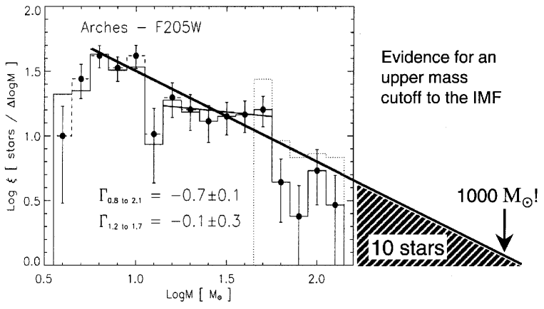
Figure 2: Stellar mass function in the Arches cluster. Taken from Figer (2002) with kind permission of the author. $\Gamma_{0.8\,{\rm to}\,2.1}=-(\alpha_{3}-1)$ for stars in the mass range log${}_{10}m\in(0.8,2.1)$.

1.4 OB associations & star clusters

Given the importance of knowing if a finite physical upper mass limit exists and how it varies with metallicity, Oey & Clarke (2005) studied the massive-star content in 9 clusters and OB associations in the MW, the LMC and the SMC. They predicted the expected masses of the most massive stars in these clusters for different upper mass limits ($120,150,200,1000\,{\rm and}\,10000\,M_{\odot}$). For all populations they found that the observed number of massive stars supports with high statistical significance the existence of a general upper mass cutoff in the range $m_{\rm max*}\in(120,\,200\,M_{\odot})$,

1.5 Concluding remarks

The general indication thus is that a physical stellar mass limit near $150\,M_{\odot}$ seems to exist. While biases due to unresolved multiples that may steepen the IMF and/or reduce the true maximal mass need to be studied further, the absence of variations of $m_{\rm max*}$ with metallicity poses a problem. A constant $m_{\rm max*}$ would only be apparent for a true variation as proposed by the theoretical models, if metal-poor environments have a larger stellar multiplicity, the effects of which would have to compensate the true increase of $m_{\rm max*}$ with metallicity.

2 Maximal stellar mass in clusters

Above we have seen that there seems to exist a universal physical stellar mass limit. However, an elementary argument suggests that star-clusters must also limit the masses of their constituent stars: A pre-star-cluster gas core with a mass $M_{\rm core}$ can, obviously, not form stars with masses $m>\epsilon\,M_{\rm core}$, where $\epsilon\approx 0.33$ is the star-formation efficiency (Lada & Lada 2003). Thus, given a freshly hatched cluster with stellar mass $M_{\rm ecl}$, stars in that cluster cannot surpass masses $m_{\rm max}=M_{\rm ecl}$, which is the identity relation corresponding to a “cluster” consisting of one massive star. Assuming the stellar IMF is a continuous density distribution function and that clusters are filled with stars distributed according to the stellar IMF, this can be generalised by stating that each cluster can have only one most massive star,

$$1=\int_{m_{\rm max}}^{m_{\rm max*}}\xi(m^{\prime})\,dm^{\prime},$$ (4)

with

$$M_{\rm ecl}(m_{\rm max})=\int_{m_{\rm low}}^{m_{\rm max}}m^{\prime}\,\xi(m^{\prime})\,dm^{\prime}$$ (5)

as a further condition, as above. These two equations need to be solved numerically and give the semi-analytical relation $m_{\rm max}\,=\,{\cal F}(M_{\rm ecl})$ (WK04). It is plotted in Fig. 3 as the thick-solid curve.

Figure 3: The thick solid line shows the dependence of the mass of the most-massive star in a cluster on the cluster mass according to the semi-analytical model. The thick dashed line shows the mean maximum stellar mass for sorted sampling (§ 2.3). The dot-dashed lines are mass-constrained random-sampling results (§ 2.2) with a physical upper mass limit of $m_{\rm max*}=150\,M_{\odot}$ (thick line) and $10^{6}\,M_{\odot}$ (thin line). Pure random sampling models (§ 2.1) are plotted as dotted lines. The thick one is sampled to $m_{\rm max*}\,=\,150\,M_{\odot}$ while the thin one up to $10^{6}\,M_{\odot}$. The thin solid line shows the identity relation, where a “cluster” consists only of one star. The dots with error bars are observed clusters, while the triangle is a result from a star-formation simulation with an SPH code (Bonnell et al. 2003). Taken from WK05a.

A literature study of clusters for which the cluster mass and the initial mass of the heaviest star can be estimated (Weidner & Kroupa 2005a, hereinafter WK05a) shows that the cluster mass indeed appears to have a limiting influence on the stellar mass within it. The observational data are plotted in Fig. 3, finding rather excellent agreement with the semi-analytical description above.

However, it would be undisputed that a stochastic sampling effect from the IMF must be present when stars form. This can be mimicked in the computer by performing various Monte-Carlo experiments (WK05a). The Monte-Carlo experiments are conducted in three different ways,

• pure random sampling (random sampling)

• mass constrained random sampling (constrained sampling)

• mass constrained random sampling with sorted adding (sorted sampling)

2.1 Random sampling

For the random sampling 10 million clusters are randomly taken from a cluster distribution with a power-law index of $\beta_{N}=2.35$ between 12 and $2.5\times 10^{7}$ stars. The relevant distribution function is the embedded-cluster star-number function (ECSNF),

$$dN_{\rm ecl}\propto N^{-\beta_{N}},$$ (6)

which is the number of clusters containing $N\in[N^{\prime},N^{\prime}+dN^{\prime})$ stars. Each cluster is then filled with $N$ stars randomly from the standard IMF (eq. 3) without a mass limit, or by imposing the physical stellar mass limit, $m\,\leq\,150\,M_{\odot}$. The stellar masses are added to get the cluster mass, $M_{\rm ecl}$. For each cluster the maximal stellar mass is searched for. For each cluster in a mass bin $M_{\rm ecl}-\Delta M_{\rm ecl}/2,M_{\rm ecl}+\Delta M_{\rm ecl}/2$ the average $m_{\rm max}$ is calculated, and the set of average $m_{\rm max}$ values define the relation

$$m_{\rm max}=m_{\rm max}^{\rm ran}(M_{\rm ecl}).$$ (7)

2.2 Constrained sampling

In this case $5\times 10^{7}$ clusters are randomly taken from the embedded-cluster mass function (ECMF),

$$\xi_{\rm ecl}(M_{\rm ecl})\propto M_{\rm ecl}^{-\beta},$$ (8)

between $5\,M_{\odot}$ (the minimal, Taurus-Auriga-type, star-forming “cluster” counting $\approx$ 15 stars) and $10^{7}\,M_{\odot}$ (an approximate maximum mass for a single stellar population that consists of one metallicity and age, Weidner, Kroupa & Larsen 2004) and again with $\beta=2.35$. Note that $\beta_{N}\approx\beta$ because the ECSNF and the ECMF only differ by a nearly-constant average stellar mass. Then stars are taken randomly from the standard IMF and added until they reach or surpass the respective cluster mass, $M_{\rm ecl}$. Afterwards the clusters are searched for their maximum stellar mass. For each cluster in a mass bin $M_{\rm ecl}-\Delta M_{\rm ecl}/2,M_{\rm ecl}+\Delta M_{\rm ecl}/2$ the average $m_{\rm max}$ is calculated, and the set of average $m_{\rm max}$ values define the relation

$$m_{\rm max}=m_{\rm max}^{\rm con}(M_{\rm ecl}).$$ (9)

2.3 Sorted sampling

For the third method again $5\times 10^{7}$ clusters are randomly sampled from the ECMF (eq. 8) between 5 $M_{\odot}$ and $10^{7}\,M_{\odot}$ and with $\beta=2.35$. However, this time the number $N$ of stars which are to populate the cluster is estimated from $N=M_{\rm ecl}/m_{\rm av}$, where $m_{\rm av}\,=\,0.36\,M_{\odot}$ is the average stellar mass for the standard IMF (eq. 3) between 0.01 $M_{\odot}$ and 150 $M_{\odot}$. These stars are added to give $M_{\rm ecl,ran}$,

$$M_{\rm ecl,ran}=\sum_{\rm N}m_{i},$$

such that $m_{i}\leq m_{i+1}$. If $M_{\rm ecl,ran}<M_{\rm ecl}$ in this first step, an additional number of stars, $\Delta N$, is picked randomly from the IMF, where $\Delta N=(M_{\rm ecl}-M_{\rm ran})/m_{\rm av}$ (we assume $m_{\rm av}=\;$constant). Again these stars are added to obtain an improved estimate of the desired cluster mass,

$${}^{2}M_{\rm ecl,ran}=\sum_{\rm N+\Delta N}m_{i},\quad m_{i}\leq m_{i+1}.$$

This is done such that ${}^{2}M_{\rm ecl,ran}\approx M_{\rm ecl}$ (details of the method will be available in WK05a). The procedure is repeated until all clusters from the ECMF are ’filled’. They are then also searched for the most massive star in each cluster, as above. For each cluster in a mass bin $M_{\rm ecl}-\Delta M_{\rm ecl}/2,M_{\rm ecl}+\Delta M_{\rm ecl}/2$ the average $m_{\rm max}$ is calculated, and the set of average $m_{\rm max}$ values define the relation

$$m_{\rm max}=m_{\rm max}^{\rm sort}(M_{\rm ecl}).$$ (10)

2.4 Comparison with observations

All three relations are plotted in Fig. 3. We noted already that the observations follow the semi-analytic relation remarkably well. Furthermore, Fig. 3 also suggests that the different Monte-Carlo schemes can be selected for. Thus, the sorted-sampling algorithm leads to virtually the same results as the semi-analytical relation, and it fits the data very well indeed. The correspondence of the sorted-sampling algorithm to the semi-analytical result is not really surprising, because the algorithm is Monte-Carlo integration of the same problem. The constrained-sampling and random-sampling algorithms, on the other hand, can be excluded with very high confidence by performing statistical tests on the observational data that are reported in detail in WK05a.

On a historical note, Larson (1982) had pointed out that more massive and dense clouds correlate with the mass of the most massive stars within them and he estimated that $m_{\rm max}=0.33\,M_{\rm cloud}^{0.43}$ (masses are in $M_{\odot}$). An updated relation was derived by Larson (2003) by comparing $m_{\rm max}$ with the stellar mass in a few clusters, $m_{\rm max}\approx 1.2\,M_{\rm cluster}^{0.45}$. Both are flatter than our semi-analytical relation, and therefore do not fit the data in Fig. 3 as well (WK05a). Elmegreen (1983) constructed a relation between cluster mass and its most massive star based on an assumed equivalence between the luminosity of the cluster population and its binding energy, for a Miller-Scalo IMF. This function is even shallower than Larson’s (2003) relation. Assuming $m_{\rm max*}=\infty$, Elmegreen (2000) solved eqs 4 above for a single Salpeter power-law stellar IMF finding a $m_{\rm max}(M_{\rm ecl})$ relation quite consistent with the data in Fig. 3 (WK05a).

3 Implications

3.1 Stellar astrophysics and the formation of star clusters

We are now in the happier situation that a physical stellar mass limit seems to have been found. But the absence of clear variation of this limit with metallicity poses a potential problem, although it may be too early to make definite statements. Further observational work on many more very young and massive clusters is needed to ascertain the findings reported here, and to quantify the multiplicity properties of massive stars, as noted above.

That our sorted-sampling algorithm for making star clusters fits the observational maximal-stellar-mass–star-cluster-mass data so well would appear to imply that clusters form in an organised fashion. The physical interpretation of the algorithm (i.e. of the Monte-Carlo integration) is that as a pre-cluster core contracts under self gravity the gas densities increase and local density fluctuations in the turbulent medium lead to low-mass star formation, perhaps similar to what is seen in Taurus-Aurigae. As the contraction proceeds and before feedback from young stars begins to disrupt the cloud, star-formation activity increases in further density fluctuations with larger amplitudes thereby forming more massive stars. The process stops when the most massive stars that have just formed supply sufficient feedback energy to disrupt the cloud. Thus, less-massive pre-cluster cloud-cores would die at a lower maximum stellar mass than more massive cores. But in all cases stellar masses are limited, $m\leq m_{\rm max}(M_{\rm ecl})\leq m_{\rm max*}$.

This scenario is nicely consistent with the hydrodynamic cluster formation calculations presented by Bonnell, Bate & Vine (2003) and Bonnell, Vine & Bate (2004), as is reported in more detail in WK05a. We note here that Bonnell et al. (2004) found their theoretical clusters to form hierarchically from smaller sub-clusters, and together with continued competitive accretion this leads to the relation $m_{\rm max}\propto M_{\rm ecl}^{2/3}$ in excellent agreement with our compilation of observational data. While this agreement is stunning, the detailed outcome of the currently available SPH modelling in terms of stellar multiplicities is not right (Goodwin & Kroupa 2005), and feedback that ultimately dominates the process of star-formation, given the generally low star-formation efficiencies observed in cluster-forming volumes, is not yet incorporated in the modelling.

3.2 Composite stellar population

The assumption has often been made that independent of the star-formation mode, the stellar distribution is sampled randomly from one invariant IMF (e.g. Elmegreen 2004). Thus, for example, $10^{5}$ clusters, each with $20$ stars, would have the same composite (i.e. combined) IMF as one cluster with $2\times 10^{6}$ stars.

However, the existence of the $m_{\rm max}(M_{\rm ecl})$ relation has profound consequences for composite populations. It immediately implies, for example, that $10^{5}$ clusters, each with $20$ stars, cannot have the same composite (i.e. combined) IMF as one cluster with $2\times 10^{6}$ stars, because the small clusters can never make stars more massive than about $1\,M_{\odot}$. Thus, galaxies, that are composite stellar populations consisting of many star clusters, most of which may be dissolved, would have steeper composite, or integrated galaxial IMFs (IGIMFs), than the stellar IMF in each individual cluster (Vanbeveren 1982; Kroupa & Weidner 2003).

The IGIMF is an integral over all star-formation events in a given star-formation “epoch” $t,t+\delta t$,

$$\xi_{\rm IGIMF}(m;t)=\int_{M_{\rm ecl,min}}^{M_{\rm ecl,max}(SFR(t))}\xi\left(m\leq m_{\rm max}\left(M_{\rm ecl}\right)\right)~{}\xi_{\rm ecl}(M_{\rm ecl})~{}dM_{\rm ecl}.$$ (11)

Thus $\xi(m\leq m_{\rm max})~{}\xi_{\rm ecl}(M_{\rm ecl})~{}dM_{\rm ecl}$ is the stellar IMF contributed by $\xi_{\rm ecl}~{}dM_{\rm ecl}$ clusters with mass near $M_{\rm ecl}$. $M_{\rm ecl,max}$ follows from the maximum star-cluster-mass vs global-star-formation-rate-of-the-galaxy relation, $M_{\rm ecl,max}={\rm fn}(SFR)$ (eq. 1 in Weidner & Kroupa 2005b, hereinafter WK05b) as derived by Weidner, Kroupa & Larsen (2004). $M_{\rm ecl,min}\,=\,5\,M_{\odot}$ is adopted in our standard modelling and corresponds to the smallest star-cluster units observed.

The “epoch” is found by WK04 to last about $\delta t=10$ Myr; in 10 Myr we find that the embedded cluster mass function is fully sampled, independent of the SFR. This time-scale compares very well indeed to the star-formation time-scale in normal galactic disks measured by Egusa, Sofue & Nakanishi (2004) using an entirely independent method, namely from the offset of HII regions from the molecular clouds in spiral-wave patterns. The time-integrated IGIMF then follows from

$$\xi_{\rm IGIMF}(m)=\int_{0}^{\tau_{\rm G}}\xi_{\rm IGIMF}(m;t)\,dt,$$ (12)

where $\tau_{\rm G}$ is the age of the galaxy under scrutiny.

Note that $\xi_{\rm IGIMF}(m)$ is the mass function of all stars ever to have formed in a galaxy, and can be used to estimate the total number of supernovae ever to have occurred, for example. $\xi_{\rm IGIMF}(m;t)$, on the other hand, includes the time-dependence through a dependency on $SFR(t)$ of a galaxy and allows one to compute the time-dependent evolution of a stellar population over the life-time of a galaxy.

Furthermore, because more-massive stellar clusters are observed to form for higher star-formation rates SFRs (Weidner, Kroupa & Larsen 2004), the ECMF is sampled to larger masses in galaxies that are experiencing high SFRs, leading to IGIMFs that are flatter than for low-mass galaxies that have had only a low-level of star-formation activity. WK05b show that the sensitivity of the IGIMF power-law index for $m\mbox{$\,\mathrel{\mathchoice{{\mbox{\lower 2.15277pt\vbox{\halign{$\mathsurround=0pt \displaystyle\hfil#\hfil$\cr>\crcr\sim\crcr}}}}}{{\mbox{\lower 2.15277pt\vbox{\halign{$\mathsurround=0pt \textstyle\hfil#\hfil$\cr>\crcr\sim\crcr}}}}}{{\mbox{\lower 2.15277pt\vbox{\halign{$\mathsurround=0pt \scriptstyle\hfil#\hfil$\cr>\crcr\sim\crcr}}}}}{{\mbox{\lower 2.15277pt\vbox{\halign{$\mathsurround=0pt \scriptscriptstyle\hfil#\hfil$\cr>\crcr\sim\crcr}}}}}}\,$}1\,M_{\odot}$ increases with decreasing $SFR$. Thus, galaxies with a small mass in stars can either form with a very low continuous SFR (appearing today as low-surface-brightness but gas-rich galaxies) or with a brief initial SF burst (dE or dSph galaxies), the IGIMF ought to vary significantly among such galaxies. Low-surface-brightness galaxies would therefore appear chemically young, while the dispersion in chemical properties ought to be larger for dwarf galaxies than for larger galaxies (WK05b). Another interesting implication is that the number of supernovae per star would be significantly smaller over cosmological times than predicted by an invariant Salpeter IMF.

As a general final comment, these new insights would imply that theoretical work on galaxy formation that relies on an invariant IMF would be wrong.

4 Further Questions

Unanswered questions regarding the formation and evolution of massive stars remain. There may be stars with $m\,\geq\,m_{\rm max*}$ which implode “invisibly” after 1 or 2 Myr. The explosion mechanism sensitively depends on the presently still rather uncertain mechanism for shock revival after core collapse (e.g. Janka 2001). Since such stars would not be apparent in massive clusters older than 2 Myr they would not affect the empirical maximal stellar mass, and $m_{\rm max*,true}$ would be unknown at present.

Furthermore, and as stated already above, stars are often in multiple systems. Especially massive stars seem to have a binary fraction of 80% or even larger (García & Mermilliod 2001) and apparently tend to be in binary systems with a preferred mass-ratio near unity. Thus, if all O stars would be in equal-mass binaries, then $m_{\rm max*\,true}\approx m_{\rm max*}/2$.

Finally, it is disconcerting that $m_{\rm max*}\,\approx\,150\,M_{\odot}$ appears to be the same for low-metallicity environments ([$\rm Fe/H$] = -0.5, R136) and metal-rich environments ([$\rm Fe/H$] = 0, Arches), in apparent contradiction to the theoretical values (Stothers 1992). Clearly, this issue needs further study.