Cosmological parameters from CMB measurements and the final 2dFGRS power spectrum

Abstract

We derive constraints on cosmological parameters using the power spectrum of galaxy clustering measured from the final two-degree field galaxy redshift survey (2dFGRS) and a compilation of measurements of the temperature power spectrum and temperature-polarization cross-correlation of the cosmic microwave background radiation. We analyse a range of parameter sets and priors, allowing for massive neutrinos, curvature, tensors and general dark energy models. In all cases, the combination of datasets tightens the constraints, with the most dramatic improvements found for the density of dark matter and the energy-density of dark energy. If we assume a flat universe, we find a matter density parameter of $\Omega_{\rm m}=0.237\pm 0.020$, a baryon density parameter of $\Omega_{\rm b}=0.041\pm 0.002$, a Hubble constant of $H_{0}=74\pm 2\;{\rm kms}^{-1}{\rm Mpc}^{-1}$, a linear theory matter fluctuation amplitude of $\sigma_{8}=0.77\pm 0.05$ and a scalar spectral index of $n_{\rm s}=0.954\pm 0.023$ (all errors show the 68% interval). Our estimate of $n_{\rm s}$ is only marginally consistent with the scale invariant value $n_{\rm s}=1$; this spectrum is formally excluded at the $95\%$ confidence level. However, the detection of a tilt in the spectrum is sensitive to the choice of parameter space. If we allow the equation of state of the dark energy to float, we find $w_{\rm DE}=-0.85_{-0.17}^{+0.18}$, consistent with a cosmological constant. We also place new limits on the mass fraction of massive neutrinos: $f_{\nu}<0.105$ at the 95% level, corresponding to $\sum m_{\nu}<1.2$ eV.

1 Introduction

Since the turn of the millennium, we have witnessed a dramatic improvement in the resolution and accuracy of measurements of fluctuations in the temperature of the cosmic microwave background radiation (CMB). The discovery of features in the power spectrum of the CMB temperature, the acoustic peaks, marked the start of a new, data-rich era in cosmology (de Bernardis et al. 2000; Hanany et al. 2000). The relative positions and heights of the acoustic peaks encode information about the values of the fundamental cosmological parameters, such as the curvature of the universe or the physical density in cold dark matter and baryons. Perhaps the most striking example of the progress achieved is the first year data from the WMAP satellite (Bennett et al. 2003; Hinshaw et al. 2003).

The CMB data alone, however, do not constrain all of the fundamental cosmological parameters to high precision. Degeneracies exist between certain combinations of parameters which lead to indistinguishable temperature fluctuation spectra (Efstathiou & Bond 1999). Some of these degeneracies can be broken by comparing theoretical models to a combination of the CMB data and other datasets, such as the power spectrum of galaxy clustering. At the same time as the new measurements of the CMB were obtained, two groundbreaking surveys of galaxies in the local Universe were being conducted. The two-degree field galaxy redshift survey (2dFGRS; Colless et al. 2001; 2003) and the Sloan Digital Sky Survey (SDSS; York et al. 2000; Abazajian et al. 2005) are substantially larger than previous redshift surveys and allow the clustering of galaxies to be measured accurately on all scales. On large scales, the connection to theoretical models is most straightforward.

Percival et al. (2001) used the power spectrum of galaxy clustering measured from the 2dFGRS to constrain the ratio of the baryon to matter density, $\Omega_{\rm b}/\Omega_{\rm m}$, and the matter density, $\Omega_{\rm m}h$. Efstathiou et al. (2002) used a compilation of pre-WMAP CMB data and the Percival et al. measurement of the galaxy power spectrum to find conclusive evidence for a non-zero cosmological constant, independent of the Hubble diagram of distant Type 1a supernovae. Percival et al. (2002) again used pre-WMAP CMB data and the early 2dFGRS power spectrum measurement to place constraints on cosmological parameters in flat models. The WMAP team also used the Percival et al. galaxy power spectrum in their estimation of cosmological parameters (Spergel et al. 2003). Other papers have also analyzed the information encoded in the 2dFGRS and SDSS power spectra (Tegmark, Zaldarriaga & Hamilton 2001; Pope et al. 2004; Tegmark et al. 2004b; Seljak et al. 2005). In view of the impact of this work, the recent completion by Cole et al. (2005) of the power-spectrum analysis of the final 2dFGRS dataset is an important development. The Cole et al. results are nearly twice as accurate as those obtained from the part-complete 2dFGRS in 2001, and a key aim of the current paper is to see how this affects the outcome of joint analyses including CMB data.

In view of these rapid improvements in our knowledge of the cosmological parameters, it is also important to take stock of precisely which parts of the model are actually being tested. Quite often, restrictive assumptions have been adopted for the background cosmology when claims are made about the constraints on a particular parameter. It is important to establish how robust the constraints really are when the data are compared with more general cosmological models.

Our goal is thus to establish firmly how well the latest CMB and large-scale structure (LSS) data determine a broad set of cosmological parameters, paying attention to how the choice of priors for parameter values and the combination of different parameters can influence the results. The outline of the paper is as follows. In Section 2, we describe the data used in our parameter estimation and set out the various parameter spaces studied. In Section 3, we present our main results for the parameter constraints obtained by comparing theoretical models to the CMB data and the galaxy power spectrum of the final 2dFGRS measured by Cole et al. (2005). We assess the impact of different choices for priors and parameter sets in Section 4. We explore the justification for using models with different numbers of free parameters in Section 5. In Section 6, we examine how the parameter constraints change when the SDSS galaxy power spectrum measured by Tegmark et al. (2004b) is used instead of the 2dFGRS power spectrum. Finally, we summarize our conclusions in Section 7.

2 The method

We now set out the approach we will take to constrain the values of the basic cosmological parameters. In Section 2.1, we list the CMB and LSS datasets that we compare against the theoretical models and explain how these datasets are modelled. The parameter sets that we will consider are defined in Section 2.2. The methodology for searching parameter space and placing constraints on parameters is set out in Section 2.3.

2.1 The datasets

In order to constrain the parameters in our cosmological model, we use a compilation of recent measurements of the CMB and the power spectrum of galaxy clustering in the local Universe:

• The WMAP first year temperature power spectrum for spherical harmonics $2\leq\ell\leq 900$ (Hinshaw et al. 2003).

• Observations of the temperature spectrum over the spherical harmonic range $900<\ell<1800$ made up to July 2002 using the Arcminute Cosmology Bolometer Array Receiver (ACBAR; Kuo et al. 2004).

• The temperature spectrum for $600<\ell<1500$ measured using the Very Small Array (VSA; Dickinson et al. 2004).

• Two years of temperature correlation data with $600<\ell<1600$ from the Cosmic Background Imager (CBI; Readhead et al. 2004).

• The WMAP first year temperature-polarization power spectrum for spherical harmonics $2\leq\ell\leq 450$ (Kogut et al. 2003).

• The power spectrum of galaxy clustering measured from the final 2dFGRS catalogue (Cole et al. 2005).

The four measurements (i-iv) of the power spectrum of temperature fluctuations in the CMB extend over the spherical harmonic range $2<\ell<1800$. Some of the available datasets extend to higher multipoles. However, we do not include these scales in our analysis, as the temperature fluctuations on such scales can be strongly affected by secondary sources. The WMAP team adopted a similar approach, augmenting the first year WMAP data with other experiments which have better angular resolution (Spergel et al. 2003). However, the VSA data were not available to the WMAP team at the time that the paper by Spergel et al. was written. Theoretical temperature-temperature and temperature-polarization spectra are computed for each model using CAMB (Lewis, Challinor & Lasenby 2000).

Cole et al. (2005) measured the power spectrum of galaxy clustering from the final 2dFGRS catalogue. The power spectrum measured for galaxies differs in a number of ways from the power spectrum for the mass predicted in linear perturbation theory: (i) Nonlinear evolution of density perturbations leads to coupling between Fourier modes, changing the shape of the power spectrum. (ii) The galaxy power spectrum is distorted by the gravitationally induced peculiar motions of galaxies when a redshift is used to infer the distance to each galaxy. (iii) The power spectrum of the galaxies could be a modified version of the power spectrum of the mass. This phenomenon is known as galaxy bias. The ratio between the galaxy and matter spectra could also change with scale. (However, we assume a constant bias over the scales considered in this paper). (iv) The power spectrum measured by Cole et al. from the 2dFGRS is the direct transform of the data, and is thus what CMB researchers would term a pseudo-spectrum. As such, it yields a convolution of the underlying galaxy power spectrum with the modulus squared of the Fourier transform of the window function of the survey.

In order to constrain cosmological parameters, these effects need to be modelled. The accuracy of the modelling requires that the comparison between theory and observation should be restricted to a limited range of scales. We use the 2dFGRS power spectrum data for $k<0.15\,h\mathrm{{Mpc^{-1}}}$ and discard measurements with $k<0.02\,h\mathrm{{Mpc^{-1}}}$ which could be affected by uncertainties in the mean density of galaxies within the survey. We follow the scheme used by Cole et al. who applied a correction for non-linearity and scale-dependent bias to the shape of $P(k)$ of the form

$$P_{\rm gal}(k)=b^{2}\frac{1+Qk^{2}}{1+Ak}\,P_{\rm lin}(k),$$ (1)

where $A=1.4$ and $Q=4.6$ are the preferred values and b is a constant bias factor. This formula is deduced by comparison with detailed numerical galaxy-formation models: these show that the value of $A$ is robust, but the exact value of $Q$ depends on galaxy type and also has some uncertainty depending on how the modelling is done. These results were used to determine a range of allowed values for $Q$, from which the value $Q=4.6$ is preferred; with this choice, robust parameter constraints are obtained if one considers maximum $k$ values beyond our limit of $0.15\,h\,{\rm Mpc}^{-1}$. For this limit, neglecting the correction entirely and simply fitting linear theory yields almost identical results to those presented here. In particular, it has no impact on the marginal indication of a deviation from $n_{\rm s}=1$.

2.2 The parameter space

In this paper, we make the basic assumption that the primordial density fluctuations were adiabatic, Gaussian and had a power law spectrum of Fourier amplitudes. As pointed out by Leach & Liddle (2003a), the CMB data prior to WMAP were of insufficient quality to justify the rejection of this simple hypothesis. Following the release of the WMAP first year results, which do have the precision required to test this model, our assumptions remain well motivated. Komatsu et al. (2003) found that the WMAP sky maps are consistent with Gaussian primordial fluctuations to a much higher precision than was attainable with COBE. Peiris et al. (2003) found that models with a spectral index varying slowly with wavenumber give slightly better fits to the WMAP data, particularly when combined with estimates of the power spectrum of the Lyman-$\alpha$ forest. However, the evidence for a running spectral index is weak and has been disputed by other groups (e.g. Bridle et al. 2003b; Slosar, Seljak & Makarov 2003; Seljak et al. 2005). Bennett et al. (2003) and Spergel et al. (2003) point out that, on large scales, a few modes of the CMB temperature power spectrum measured by WMAP lie below the predictions of the standard $\Lambda$CDM model. One interpretation of this apparent discrepancy is that new physics may be needed (e.g. Bridle et al. 2003a; Efstathiou 2003). However, several studies have argued that the disagreement is actually less significant than was first claimed (Gaztañaga et al. 2003; de Oliveira-Costa et al. 2003; Efstathiou 2004).

¿From the above starting point, the cosmological model we consider is defined by eleven parameters:

$$\mathbf{P\equiv(}\Omega_{k},\omega_{\rm dm},\omega_{\rm b},f_{\rm\nu},w_{\rm DE},\tau,n_{\rm s},A_{\rm s},r,b,\Theta).$$ (2)

There are eight further basic quantities whose values can be derived given the above set:

$$\mathbf{P_{\rm derived}\equiv(}\Omega_{\rm DE},h,\Omega_{\rm m},\sigma_{8},z_{\rm re},t_{0},\sum m_{\nu},n_{\rm t}).$$ (3)

We now go through the parameters in these lists, defining each one and explaining how the values of the derived parameters are obtained.

The are five quantities that describe the homogeneous background cosmology through various contributions to the mass-energy density. These are, in units of the critical density: $\Omega_{k}$, which describes the curvature of the universe; $\Omega_{\rm DE}$, the energy-density of the dark energy; $\omega_{\rm dm}\equiv\Omega_{\rm dm}h^{2}$, the density of the dark matter (where $\Omega_{\rm dm}=\Omega_{\rm cdm}+\Omega_{\nu}$ is the sum of the cold and hot dark matter components and $h$ is Hubble’s constant in units of $100\,{\rm kms}^{-1}{\rm Mpc}^{-1}$); $\omega_{\rm b}\equiv\Omega_{\rm b}h^{2}$, the baryon density; and $f_{\rm\nu}=\Omega_{\rm\nu}/\Omega_{\rm dm},$ the fraction of the dark matter in the form of massive neutrinos. The sum of neutrino masses is given by $\sum m_{\nu}$. The matter density parameter is given by $\Omega_{\rm m}=\Omega_{\rm dm}+\Omega_{\rm b}$. The value of the Hubble constant is derived from $h=\sqrt{(\omega_{\rm dm}+\omega_{\rm b})/\Omega_{\rm m}}$. The energy density of the dark energy is set by $\Omega_{\rm DE}=1-\Omega_{\rm m}-\Omega_{k}$. The dark energy component is assumed to have an equation of state that is independent of redshift, with the ratio of pressure to density given by $w_{\rm DE}$.

There are four quantities that describe the form of the initial fluctuations; the spectral indices, $n_{\rm s}$ and $n_{\rm t}$, and the primordial amplitudes, $A_{\rm s}$ and $rA_{\rm s}$, of scalar and tensor fluctuations respectively. These parameter values are quoted at the ‘pivot’ scale wavenumber of $k=0.05\,{\rm Mpc}^{-1}$. We can translate the results obtained for $A_{\rm s}$ into a constraint on the more familiar parameter $\sigma_{8}$, the rms linear perturbation theory variance in spheres of radius $8~{}h^{-1}$Mpc, using the matter fluctuation transfer function. Note that when we consider tensor modes, we make the slow-roll assumption that $n_{\rm t}=-r/8$.

The bias factor, $b\equiv\sqrt{P_{\rm gal}(k)/P_{\rm DM}(k)}$, describes the difference in amplitude between the galaxy power spectrum and that of the underlying dark matter. The value of $b$ is marginalized over, using the analytic expression given in Appendix F of Lewis & Bridle (2002). We assume that the reionization of the neutral intergalactic medium occurred instantaneously, with an optical depth given by $\tau$; the redshift of reionization, $z_{\rm re}$, depends upon a combination of parameters (see Table 1 of Tegmark et al. 2004b). The age of the universe is $t_{0}$.

Finally, $\Theta$ gives the ratio of the sound horizon scale at the epoch of decoupling to the angular diameter distance to the corresponding redshift and replaces the Hubble constant as a base parameter (Kosowsky, Milosavljevic & Jimenez 2002). We have chosen to use this parameter, rather than, for example, the energy density in dark energy, since it has a posterior distribution that is close to Gaussian. This reduces degeneracies between parameters and results in a faster convergence of our search of parameter space (see Section 2.3), compared with studies in which parameters such as $\Omega_{\rm DE}$, which does not have a Gaussian posterior distribution, are allowed to vary. This approach is a standard practice even though, usually, the final results are expressed in terms of more familiar parameters such as $\Omega_{\rm DE}$ or $h$. However, care must be taken when comparing our results with those from studies which have assumed flat priors on different parameters in their Bayesian analysis. Such choices may affect the final results in a way that is difficult to quantify.

We do not attempt to vary all eleven parameters of the model at once. Such an approach would lead to a mixture of poor estimates of the values of individual parameters and constraints on various combinations of parameters. As we are primarily interested in deriving the best possible constraints on individual parameters, we instead consider subsets of parameter space, varying five, six or seven parameters at a time. Of the remaining parameters, some are held at fixed values and the others are referred to as derived parameters. The values of the derived parameters follow from the values of other parameters, once the assumptions made in each parameter space have been taken into account. We will now set out each of our parameter spaces in turn, stating which parameters are varied and which are held fixed. In all cases, the bias parameter, $b$, is marginalized over, so we do not include this in the list of parameters whose values are constrained.

In the simplest case, we vary five parameters which we refer to as the ‘basic-five’ (b5) parameter set. The following parameters are allowed to float:

$$\mathbf{P^{5}_{\rm varied}\equiv(}\omega_{\rm dm},\omega_{\rm b},\tau,A_{\rm s},\Theta).$$ (4)

The values of the fixed parameters in the basic-five model are:

$$\mathbf{P^{5}_{\rm fixed}\equiv(}\Omega_{\rm k}=0,f_{\rm\nu}=0,w_{\rm DE}=-1,n_{\rm s}=1,r=0).$$ (5)

The results of this model are discussed in Section 3.2.

The basic-five set is expanded to allow the value of the scalar spectral index to float, giving the basic-six (b6) model (see Section 3.3):

$$\mathbf{P^{6}_{\rm varied}\equiv(}\omega_{\rm dm},\omega_{\rm b},\tau,n_{\rm s},A_{\rm s},\Theta).$$ (6)

The fixed parameters in the basic-six model are:

$$\mathbf{P^{6}_{\rm fixed}\equiv(}\Omega_{\rm k}=0,f_{\rm\nu}=0,w_{\rm DE}=-1,r=0).$$ (7)

Table 1: The parameter space probed in our analysis. We assume a flat prior in each case. We do not vary the values of all parameters at the same time; the parameter spaces that we consider are set out in Section 2.2.

Parameter	Allowed range
$\Omega_{k}$	$-$0.3 – 0.3
$\omega_{\rm dm}$	0.01 – 0.99
$\omega_{\rm b}$	0.005 – 0.1
$f_{\rm\nu}$	0 – 0.5
$w_{\rm DE}$	$-$2. – 0
$\tau$	0 – 0.8
$n_{\rm s}$	0.5 – 1.5
$\log_{10}(10^{10}A_{\rm s})$	2.7 – 4.0
$r$	0 – 1
$\Theta$	0.5 – 10

We also consider four parameter spaces in which one additional parameter is constrained along with the basic-six set. In Section 3.3, the additional parameter is the mass fraction of massive neutrinos, $f_{\nu}$:

$$\mathbf{P^{6+f_{\nu}}_{\rm varied}\equiv(}\omega_{\rm dm},\omega_{\rm b},f_{\nu},\tau,n_{\rm s},A_{\rm s},\Theta).$$ (8)

The fixed parameters in this case are:

$$\mathbf{P^{6+f_{\nu}}_{\rm fixed}\equiv(}\Omega_{\rm k}=0,w_{\rm DE}=-1,r=0).$$ (9)

In Section 3.4, the curvature of the universe, $\Omega_{k}$ is allowed to float and the fraction of massive neutrinos is once again held fixed:

$$\mathbf{P^{6+\Omega_{k}}_{\rm varied}\equiv(}\Omega_{k},\omega_{\rm dm},\omega_{\rm b},\tau,n_{\rm s},A_{\rm s},\Theta).$$ (10)

$$\mathbf{P^{6+\Omega_{k}}_{\rm fixed}\equiv(}f_{\nu}=0,w_{\rm DE}=-1,r=0).$$ (11)

In Section 3.5, the equation of state of the dark energy is varied:

$$\mathbf{P^{6+w_{\rm DE}}_{\rm varied}\equiv(}\omega_{\rm dm},\omega_{\rm b},w_{\rm DE},\tau,n_{\rm s},A_{\rm s},\Theta).$$ (12)

In this case, the fixed parameters are:

$$\mathbf{P^{6+w_{\rm DE}}_{\rm fixed}\equiv(}\Omega_{\rm k}=0,f_{\nu}=0,r=0).$$ (13)

Finally, in Section 3.6, the constraints on tensor modes are investigated:

$$\mathbf{P^{6+r}_{\rm varied}\equiv(}\omega_{\rm dm},\omega_{\rm b},\tau,n_{\rm s},A_{\rm s},r,\Theta),$$ (14)

with the fixed parameters given by:

$$\mathbf{P^{6+r}_{\rm fixed}\equiv(}\Omega_{\rm k}=0,f_{\nu}=0,w_{\rm DE}=-1).$$ (15)

Table 1 summarizes the ranges considered for different cosmological parameters when their values are allowed to vary.

2.3 Constraining parameters

The prohibitive computational cost of generating CMB power spectra and matter transfer functions for all the grid points in a multidimensional parameter space has driven the development of codes that sample the space selectively, guided by the shape of the likelihood surface. We use a Markov Chain Monte Carlo (MCMC) approach to search the parameter space of the cosmological model (for a recent example of the application of the MCMC algorithm to cosmological applications, see Percival 2004). In brief, this algorithm involves conducting a series of searches of parameter space called chains. The chains are started at widely separated locations within the space. The next link in a chain is made in a randomly chosen direction in the parameter space. The new link becomes part of the chain if it passes a test devised by Metropolis et al. (1953); in summary, links for which the likelihood increases are always retained, otherwise acceptance occurs with a probability that is the ratio of likelihoods between the new and old links. If a link is rejected, a new randomly generated step is taken in the parameter space. This rate of hopping between pairs of points in parameter space satisfies the principle of detailed balance, so that the chains should asymptotically take up a stationary probability distribution that follows the likelihood surface. The advantage of this method is that marginalization (i.e. integration of the posterior distribution over uninteresting parameters) is extremely easy: one simply adds up the number of links that fall within binned intervals of the interesting parameter values (see the appendices in Lewis & Bridle 2002).

The results presented in this paper were generated with the publicly available CosmoMC code of Lewis & Bridle (2002). We have compared the parameter constraints obtained with this code with those from an independent code written by one of us (WJP), and find excellent agreement between the two sets of results. CosmoMC uses the CAMB package to compute power spectra for the CMB and matter fluctuations (Lewis, Challinor & Lasenby 2000). Our analysis was carried out in parallel on the Cosmology Machine at Durham University. For each parameter set considered, we ran twenty separate chains using the Message Passing Interface (MPI) convergence criterion to stop the chains when the Gelman and Rubin (1992) statistic $R<1.02$, which is a significantly more stringent criterion than is usually adopted (Verde et al. 2003; Seljak et al. 2005). The length of chain generated before the above convergence criterion is achieved depends upon the datasets used. For CMB data alone, the chains typically have on the order of 10,000 links; in the case of CMB plus the 2dFGRS $P(k)$, convergence can be reached more quickly. In total, our calculations have accounted for the equivalent of more than 30 CPU years on a single processor.

3 Results

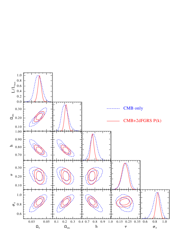
Figure 1: Marginalized posterior likelihoods for the cosmological parameters in the basic-five model determined from CMB information only (dashed lines) and CMB+2dFGRS $P(k)$ (solid lines). The diagonal shows the likelihood for individual parameters; the other panels show the likelihood contours for pairs of parameters, marginalizing over the other parameters. The contours show $-2\Delta\ln(L/L_{\rm max})=2.3$ and $6.17$.

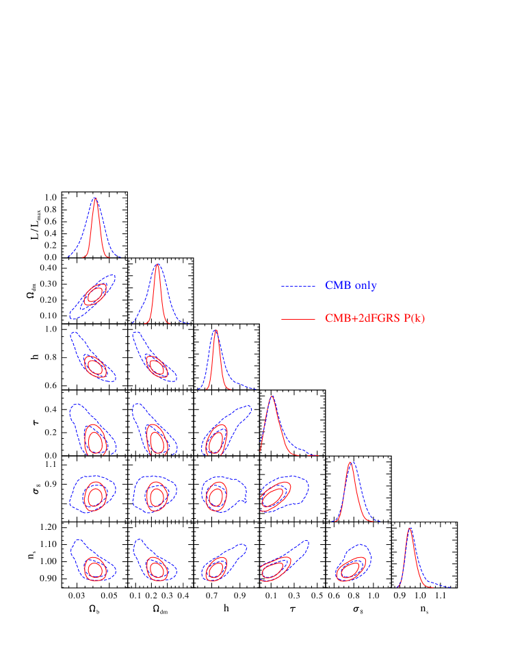
Figure 2: Marginalized posterior likelihoods for the cosmological parameters in the basic-six model determined from CMB information only (dashed lines) and CMB plus 2dFGRS $P(k)$ (solid lines).

In this Section, we carry out a systematic study of the constraints placed on the values of cosmological parameters by the CMB and LSS datasets listed in Section 2.1. We vary three aspects of the comparison: (i) The datasets used. We compare constraints obtained from the CMB data alone (Table 2) with those obtained from the CMB data in combination with the 2dFGRS power spectrum (Table 3). This allows us to see which parameters are constrained more strongly when the CMB data are combined with a measurement of the galaxy power spectrum. (ii) The number of parameters varied. We consider models in which 5, 6 or 7 parameters are allowed to float whilst the other parameters are held at fixed values (see Section 2.2 for the definition of our parameter spaces). (iii) The combination of parameters. In our 7 parameter models, we add one additional parameter to our basic-six set (Eq. 6) and explore how different choices for this additional parameter can affect the parameter constraints.

Our results are summarized in Tables 2 and 3. In the top half of each table, we show the values of the fundamental parameters. These are either the range of values derived by comparison with a particular dataset or the value that a parameter is fixed at in the analysis, as explained in Section 2.2. In the lower part of the tables, we quote the values of other useful parameters (as listed in Eq. 3). These parameters are not varied directly in our analysis. However, their values can be derived from the results in the upper half of the table, as explained in Section 2.2.

In Section 3.1, we present the results for a minimal cosmological model with five parameters, the basic-five set. In Section 3.2, we consider six parameters, the basic-six set, allowing the spectral index of scalar fluctuations to float. Sections 3.3 to 3.6 are devoted to seven parameter models, with different choices for the ‘final’ parameter that augments the basic-six set, as follows: Section 3.3 the mass fraction of massive neutrinos, $f_{\rm\nu}$, Section 3.4 non-flat models, Section 3.5 the dark energy equation of state, $w_{\rm DE}$, Section 3.6 the addition of tensor perturbations.

In the results tables, unless otherwise stated, we quote errors that enclose $68\%$ of the probability around the mean value of each parameter. In the subsequent figures showing the marginalized posterior likelihood surface for two parameters, the contours mark the locus where $-2\Delta\ln\left({\cal L}/{\cal L}_{\rm max}\right)=2.30$ and $6.17$, corresponding to the 68% and 95% limits respectively; for the case of a Gaussian likelihood, these contours correspond to the ‘1$\sigma$’ and ‘2$\sigma$’ limits for two degrees of freedom.

Table 2: Marginalized 68% interval constraints (unless stated otherwise) on cosmological parameters obtained using CMB information only for the different hypothesis and parameter sets analysed. The models are defined in Section 2.2.

	b5	b6	b6 + $f_{\nu}$	b6 + $\Omega_{k}$	b6 + $w_{\rm DE}$	b6 + $r$
$\Omega_{k}$	0	0	0	$-0.074^{+0.049}_{-0.052}$	0	0
$\Theta$	$1.0449^{+0.0041}_{-0.0042}$	$1.0420^{+0.0052}_{-0.0052}$	$1.0428^{+0.0059}_{-0.0058}$	$1.0427^{+0.0063}_{-0.0062}$	$1.0426^{+0.0052}_{-0.0052}$	$1.0433^{+0.0051}_{-0.0051}$
$\omega_{\rm dm}$	$0.101^{+0.011}_{-0.011}$	$0.105^{+0.013}_{-0.013}$	$0.113^{+0.014}_{-0.015}$	$0.095^{+0.019}_{-0.026}$	$0.105^{+0.013}_{-0.013}$	$0.099^{+0.010}_{-0.011}$
$\omega_{\rm b}$	$0.0239^{+0.0007}_{-0.0007}$	$0.0229^{+0.0012}_{-0.0013}$	$0.0226^{+0.0015}_{-0.0016}$	$0.0238^{+0.0032}_{-0.0022}$	$0.0231^{+0.0013}_{-0.0013}$	$0.0236^{+0.0013}_{-0.0013}$
$f_{\nu}$	0	0	$<0.182$ (95%)	0	0	0
$\tau$	$0.217^{+0.037}_{-0.036}$	$0.150^{+0.084}_{-0.078}$	$0.161^{+0.101}_{-0.091}$	$0.24^{+0.24}_{-0.16}$	$0.142^{+0.074}_{-0.073}$	$0.126^{+0.062}_{-0.062}$
$w_{\rm DE}$	$-1$	$-1$	$-1$	$-1$	$-0.93^{+0.49}_{-0.47}$	$-1$
$n_{\rm s}$	1	$0.970^{+0.033}_{-0.033}$	$0.957^{+0.045}_{-0.047}$	$1.00^{+0.11}_{-0.07}$	$0.974^{+0.038}_{-0.037}$	$0.994^{+0.033}_{-0.033}$
$\log_{10}(10^{10}A_{\rm s})$	$3.270^{+0.059}_{-0.058}$	$3.14^{+0.16}_{-0.15}$	$3.14^{+0.19}_{-0.18}$	$3.29^{+0.42}_{-0.28}$	$3.12^{+0.14}_{-0.14}$	$3.07^{+0.13}_{-0.13}$
$r$	0	0	0	0	0	$<0.52$ (95%)
$\Omega_{\rm DE}$	$0.793^{+0.039}_{-0.038}$	$0.762^{+0.056}_{-0.055}$	$0.68^{+0.10}_{-0.10}$	$0.63^{+0.18}_{-0.17}$	$0.71^{+0.12}_{-0.14}$	$0.798^{+0.041}_{-0.042}$
$t_{0}/{\rm Gyr}$	$13.38^{+0.12}_{-0.12}$	$13.58^{+0.26}_{-0.25}$	$14.03^{+0.47}_{-0.44}$	$16.3^{+1.4}_{-1.5}$	$13.79^{+0.50}_{-0.45}$	$13.43^{+0.25}_{-0.26}$
$\Omega_{\rm m}$	$0.207^{+0.038}_{-0.039}$	$0.237^{+0.055}_{-0.056}$	$0.32^{+0.10}_{-0.10}$	$0.44^{+0.21}_{-0.20}$	$0.28^{+0.14}_{-0.12}$	$0.202^{+0.041}_{-0.042}$
$\sigma_{8}$	$0.840^{+0.069}_{-0.069}$	$0.800^{+0.073}_{-0.072}$	$0.63^{+0.12}_{-0.12}$	$0.776^{+0.076}_{-0.072}$	$0.75^{+0.18}_{-0.18}$	$0.706^{+0.093}_{-0.097}$
$z_{\rm re}$	$19.6^{+2.1}_{-2.1}$	$15.0^{+5.6}_{-5.1}$	$15.9^{+6.8}_{-5.9}$	$18.6^{+9.7}_{-7.7}$	$14.5^{+5.1}_{-5.0}$	$15.4^{+5.3}_{-5.3}$
$h$	$0.783^{+0.040}_{-0.040}$	$0.747^{+0.055}_{-0.056}$	$0.674^{+0.078}_{-0.082}$	$0.54^{+0.11}_{-0.11}$	$0.72^{+0.18}_{-0.17}$	$0.786^{+0.053}_{-0.052}$
$\sum{m_{\nu}}/\rm{eV}$	0	0	$<2.09$	0	0	0

Table 3: Marginalized 68% interval constraints (unless stated otherwise) on cosmological parameters obtained using information from CMB and the 2dFGRS power spectrum for the different hypothesis and parameter sets analysed. The models are defined in Section 2.2.

	b5	b6	b6 + $f_{\nu}$	b6 + $\Omega_{k}$	b6 + $w_{\rm DE}$	b6 + $r$
$\Omega_{k}$	0	0	0	$-0.029^{+0.018}_{-0.018}$	0	0
$\Theta$	$1.0453^{+0.0038}_{-0.0037}$	$1.0403^{+0.0046}_{-0.0045}$	$1.0411^{+0.0050}_{-0.0046}$	$1.0458^{+0.0079}_{-0.0076}$	$1.0422^{+0.0055}_{-0.0055}$	$1.0425^{+0.0049}_{-0.0049}$
$\omega_{\rm dm}$	$0.1046^{+0.0055}_{-0.0053}$	$0.1051^{+0.0046}_{-0.0047}$	$0.1100^{+0.0062}_{-0.0067}$	$0.083^{+0.015}_{-0.015}$	$0.097^{+0.011}_{-0.011}$	$0.1037^{+0.0050}_{-0.0050}$
$\omega_{\rm b}$	$0.0240^{+0.0006}_{-0.0006}$	$0.0225^{+0.0010}_{-0.0010}$	$0.0224^{+0.0012}_{-0.0011}$	$0.0252^{+0.0033}_{-0.0030}$	$0.0233^{+0.0016}_{-0.0016}$	$0.0233^{+0.0011}_{-0.0011}$
$f_{\nu}$	0	0	$<0.105$ (95%)	0	0	0
$\tau$	$0.208^{+0.034}_{-0.034}$	$0.118^{+0.057}_{-0.056}$	$0.143^{+0.076}_{-0.071}$	$0.33^{+0.18}_{-0.19}$	$0.174^{+0.107}_{-0.095}$	$0.109^{+0.053}_{-0.053}$
$w_{\rm DE}$	$-1$	$-1$	$-1$	$-1$	$-0.85^{+0.18}_{-0.17}$	$-1$
$n_{\rm s}$	1	$0.954^{+0.023}_{-0.023}$	$0.957^{+0.031}_{-0.029}$	$1.05^{+0.10}_{-0.10}$	$0.985^{+0.053}_{-0.046}$	$0.979^{+0.028}_{-0.028}$
$\log_{10}(10^{10}A_{\rm s})$	$3.268^{+0.060}_{-0.060}$	$3.06^{+0.12}_{-0.12}$	$3.11^{+0.15}_{-0.14}$	$3.44^{+0.35}_{-0.37}$	$3.16^{+0.20}_{-0.18}$	$3.05^{+0.11}_{-0.11}$
$r$	0	0	0	0	0	$<0.41$ (95%)
$\Omega_{\rm DE}$	$0.781^{+0.019}_{-0.020}$	$0.763^{+0.020}_{-0.020}$	$0.718^{+0.042}_{-0.037}$	$0.796^{+0.040}_{-0.040}$	$0.759^{+0.024}_{-0.024}$	$0.778^{+0.021}_{-0.022}$
$t_{0}/{\rm Gyr}$	$13.39^{+0.11}_{-0.11}$	$13.69^{+0.19}_{-0.20}$	$13.94^{+0.26}_{-0.26}$	$14.97^{+0.77}_{-0.79}$	$13.70^{+0.26}_{-0.26}$	$13.54^{+0.23}_{-0.23}$
$\Omega_{\rm m}$	$0.219^{+0.020}_{-0.019}$	$0.237^{+0.020}_{-0.020}$	$0.282^{+0.037}_{-0.042}$	$0.234^{+0.028}_{-0.027}$	$0.241^{+0.024}_{-0.024}$	$0.224^{+0.022}_{-0.022}$
$\sigma_{8}$	$0.863^{+0.037}_{-0.037}$	$0.773^{+0.054}_{-0.053}$	$0.678^{+0.073}_{-0.072}$	$0.817^{+0.077}_{-0.079}$	$0.711^{+0.098}_{-0.099}$	$0.769^{+0.053}_{-0.062}$
$z_{\rm re}$	$19.2^{+2.1}_{-2.1}$	$13.1^{+4.3}_{-4.3}$	$15.1^{+5.2}_{-5.1}$	$22.6^{+6.2}_{-7.9}$	$16.1^{+6.2}_{-5.8}$	$12.1^{+4.1}_{-4.2}$
$h$	$0.776^{+0.020}_{-0.019}$	$0.735^{+0.022}_{-0.023}$	$0.691^{+0.038}_{-0.038}$	$0.684^{+0.035}_{-0.035}$	$0.708^{+0.062}_{-0.058}$	$0.755^{+0.028}_{-0.029}$
$\sum{m_{\nu}}/\rm{eV}$	0	0	$<1.16$ (95%)	0	0	0

3.1 The simplest case – five parameters

We first concentrate on the simplest possible model that gives an accurate description of the data sets, the basic-five parameter space defined by Eqs. 4 and 5. This model does a remarkably good job of reproducing the CMB data, with tight constraints obtained on the values of the subset of five cosmological parameters varied, as shown by the dashed lines in Fig. 1 and column 2 of Table 2. It is clear from Fig. 1 and Table 3, that, when the 2dFGRS $P(k)$ is included, the results show an impressive consistency with those obtained from the CMB data alone. For example, in the case of the physical density of dark matter, $w_{\rm dm}$, the central values derived when comparing to CMB data alone and to CMB plus 2dFGRS agree well within the uncertainties. However, in a number of cases, there is a significant improvement in the parameter constraints obtained when the 2dFGRS $P(k)$ data are included. For example, the range of $w_{\rm dm}$ values derived is narrower by a factor of 2 when the 2dFGRS $P(k)$ is included in the fit, as the LSS data breaks the horizon-angle degeneracy arising from CMB models with the same position of the first peak in the angular power spectrum (e.g. Percival et al. 2002). A similar reduction in uncertainty occurs for the derived parameters $\sigma_{8}$ and $h$. The CMB power spectrum is sensitive to the parameter $\omega_{\rm dm}=\Omega_{\rm dm}h^{2}$ whereas the matter $P(k)$ depends on the parameter combination $\Omega_{\rm dm}h$. The incorporation of $P(k)$ into the analysis helps to break the degeneracy between $\Omega_{\rm dm}$ and $h$ present in the theoretical predictions for the CMB, thus tightening the constraints on these parameters, as well as on $\omega_{\rm dm}$. Cole et al. (2005) used the 2dFGRS $P(k)$ to place constraints on the parameter combinations $\Omega_{\rm m}h$ and $\Omega_{\rm b}/\Omega_{\rm m}$, and, in conjunction with the WMAP temperature power spectrum, on $\Omega_{\rm m}$. The model that Cole et al. considered is a restricted version of our basic-five model (they assumed $h=0.72$). It is reassuring to note that our results are in excellent agreement with those obtained by Cole et al.; in particular, we confirm their finding of a matter density significantly below the canonical $\Lambda$CDM value of $\Omega_{\rm m}=0.3$. The success of this simple model in describing the current CMB and LSS data is remarkable. This ‘minimalist model’ does a perfectly good job of accounting for the form of the most precise probes of the cosmological world model that are available to us today.

3.2 Six parameters – including the scalar spectral index

We now expand our model to allow variations in the scalar spectral index, $n_{\rm s}$, which we call the ‘basic-six’ parameter space (defined by Eqs. 6 and 7). Fig. 2 shows the marginalized likelihoods for this parameter set (along the diagonal), together with the two dimensional likelihood contours for different combinations of parameters. The results are shown using the CMB data alone (dashed lines) and for CMB plus 2dFGRS $P(k)$ (solid lines). The additional degree of freedom gives rise to a well known degeneracy that involves all six parameters and which is seen most clearly in the optical depth to last scattering, $\tau$, and the spectral index and amplitude of scalar fluctuations, $n_{\rm s}$ and $A_{\rm s}$ respectively. This degeneracy leads to the production of similar power spectra as the parameter values, with the exception of $\omega_{\rm dm}$, are increased (see Tegmark et al. 2004b for a full description of how the degeneracy works in practice). Table 2 shows that in the case of the CMB data alone, the results for the best fitting parameters in the basic-six case are, for the most part, very similar to those obtained for the basic-five parameter set. The two exceptions are $\tau$ and $A_{\rm s}$, for which slightly lower values are obtained in the basic-six case. This is also a consequence of the above degeneracy, since, as the data prefer $n_{\rm s}<1$, the best fitting values for $\tau$ and $A_{\rm s}$ also decrease. Another consequence of the degeneracy is to broaden the allowed regions compared with those obtained for the basic-five parameter set. The 2dFGRS power spectrum helps to break this degeneracy, particularly by tightening the constraints on $w_{\rm dm}$. The results listed in column 3 of Table 3 show that the marginalized constraints obtained in this case are in complete agreement with those in the CMB only case, but with tighter allowed ranges. This reinforces the consistency of the results obtained from CMB alone and CMB plus 2dFGRS $P(k)$ that we found in the basic-five case.

One particularly remarkable result is the recovered value of the spectral index of scalar perturbations, $n_{\rm s}$. In the case of CMB data alone, we obtain $n_{\rm s}=0.970^{+0.033(0.110)}_{-0.033(0.052)}$ where the errors correspond to 68% (95%), fully consistent with $n_{\rm s}=1$. However, with the smaller errors afforded by combining the CMB data with the 2dFGRS $P(k)$ data, we obtain $n_{\rm s}=0.954^{+0.023(0.054)}_{-0.023(0.040)}$. This measurement of the scalar perturbation spectral index is consistent with scale invariant value $n_{\rm s}=1$ at the $95\%$ level. Any detection of a deviation from scale invariance would have strong implications for the inflationary paradigm, and we discuss this result in more detail below in Section 5.2.

3.3 Six parameters plus the mass fraction of massive neutrinos

Massive neutrinos were ruled out a generation ago as the sole constituent of the dark matter, on the basis of N-body simulations of the formation of large scale structure in hot dark matter universes (Frenk, White & Davis 1983). However, interest in massive neutrinos has been resurrected recently with the resolution of the solar neutrino problem and the advent of precision measurements of the galaxy power spectrum. The detection of other flavours of neutrino in addition to the electron neutrino in the flux of neutrinos from the Sun suggests that neutrinos can oscillate between flavours (Ahmad et al. 2001). This in turn implies that the three known types of neutrino have a non-zero mass, although measurements of the degree of flavour mixing set limits on the mass-squared differences between the neutrino flavours rather than on their absolute masses. The most extreme (and perhaps most plausible) case is where the lightest mass eigenvalue is negligibly small, in which case the sum of neutrino masses is dominated by the heaviest eigenvalue: $\sum{m_{\nu}}\simeq m_{3}\simeq 0.045$ eV (for a recent review see Barger et al. 2003). The only way in which $\sum{m_{\nu}}$ can greatly exceed this figure is if the mass hierarchy is almost degenerate; we therefore assume three species of equal mass in what follows. Absolute measurements of neutrino mass can be obtained from Tritium beta decay experiments. At present, such experiments provide a limit on the sum of the neutrino masses of $\sum{m_{\nu}}<6.6$ eV at the 2$\sigma$ level (Weinheimer 2002).

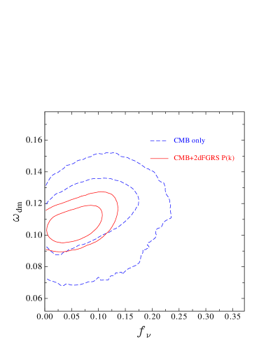
Figure 3: The marginalized posterior likelihood in the $f_{\nu}-\omega_{\rm dm}$ plane for the basic-six+$f_{\nu}$ parameter set. The dashed lines show the 68% and 95% contours obtained in the CMB only case. The solid contours show the corresponding results obtained in the CMB plus 2dFGRS $P(k)$ case.

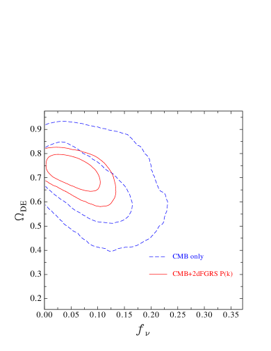
Figure 4: The marginalized posterior likelihood in the $f_{\nu}-\Omega_{\rm DE}$ plane for the basic-six+$f_{\nu}$ parameter set. The dashed lines show the 68% and 95% contours obtained in the CMB only case. The solid contours show the parameter constraints obtained for combined CMB and 2dFGRS $P(k)$ datasets.

Currently, the most competitive limits on neutrino masses are obtained through the comparison of CMB and LSS data with theoretical models (Hu et al. 1998; Elgaroy et al. 2002; Hannestad 2002). In the early universe, when neutrinos were still relativistic, they free-streamed out of density perturbations, damping overdensities in the baryons and cold dark matter. This smearing effect stops once neutrinos become non-relativistic; in this case, free-streaming only suppresses power on scales smaller than the horizon at this epoch, which depends on neutrino mass.

The CMB temperature power spectrum is only weakly dependent on the neutrino mass fraction, $f_{\nu}$, since at the epoch of last scattering neutrinos with eV masses behave in a similar fashion to cold dark matter. So, CMB data alone do a poor job of constraining the neutrino mass fraction. Moreover, the response of the CMB power spectrum to variations in $f_{\nu}$ is limited to the higher multipoles ($\ell\geq 700$) and so the first year WMAP data alone cannot give good constraints on this quantity (see the results of Tegmark et al. 2004b). Our constraints in the CMB only case arise mainly due to data other than WMAP which probe smaller angular scales and therefore higher multipoles. On the other hand, the impact of massive neutrinos on the shape of the matter power spectrum is much more pronounced. The combination of CMB data with a measurement of the mass power spectrum can therefore give a much tighter constraint on the mass fraction of neutrinos; the shape of $P(k)$ constrains the value of $f_{\nu}$ while the CMB data sets the values of the parameters that are degenerate with $f_{\nu}$.

Using CMB data only, we find $f_{\nu}<0.182$ at $95\%$. When the 2dFGRS $P(k)$ is included this becomes $f_{\nu}<0.105$ at $95\%$. Our results can be converted into constraints on the sum of the three neutrino masses using $\sum{m_{\nu}}=\omega_{\rm dm}f_{\nu}\,94.4\,\mathrm{eV}$ (assuming standard freezeout and that neutrinos are Majorana particles) to obtain the following limits: $\sum{m_{\nu}}<2.09\,$ eV at $95\%$ in the CMB only case, $\sum{m_{\nu}}<1.16\,\rm{eV}$ at $95\%$ for CMB data plus the 2dFGRS $P(k)$.

Elgaroy et al. (2002) used the Percival et al. (2001) measurement of the 2dFGRS power spectrum to constrain the neutrino mass and found $\sum m_{\nu}<2.2\,$ eV (95%), assuming $n_{s}=1$ and a restrictive prior on $\Omega_{\rm m}$. Our results also represent a substantial improvement over those reported by Tegmark et al. (2004b), who combined the first year WMAP data with the SDSS power spectrum to constrain a similar set of parameters to those we consider and found a $95\%$ limit of $\sum{m_{\nu}}\leq 1.7$ eV. Our results for $f_{\nu}$ provide an important illustration of the need to augment the WMAP data, which is the most accurate available for $\ell\leq 600$, with measurements conducted at higher angular resolution, allowing significant improvements in the constraints attainable on certain parameters.

It is possible to obtain a stronger limit from CMB+LSS studies if amplitude information is also used: a neutrino fraction reduces the overall growth rate as well as changing the shape of the matter power spectrum. This constraint was used in the year-1 WMAP analysis, and was important in reaching the tight constraint of $\sum m_{\nu}<0.7$ eV (Spergel et  al. 2003; Verde et al. 2003). This analysis required the use of the 2dFGRS bispectrum in addition to $P(k)$ (Verde et al. 2002; for a determination with the final 2dFGRS see Gaztañaga et al. 2005); we have preferred not to use this information at the present time, since it has not been subject to the same degree of detailed simulation as $P(k)$. The limit on the neutrino mass can also be tightened if a measurement of the linear theory matter power spectrum is available at higher wavenumbers than can be probed with the galaxy power spectrum. Seljak et al. (2005) used the power spectrum of the Ly-$\alpha$ forest and the SDSS $P(k)$, with a prior on the optical depth to last scattering of $\tau<0.3$ (see later), to obtain $\sum{m_{\nu}}<0.42$ eV. The extraction of the linear theory power spectrum of matter fluctuations from the Lyman-$\alpha$ forest remains controversial, so we do not address the use of this dataset here (Croft et al. 2002; Gnedin & Hamilton 2002; McDonald et al. 2005).

The only work to have reported a measurement of a non-zero neutrino mass rather than an upper limit is Allen et al. (2003). These authors combined galaxy cluster data with CMB data and an earlier version of the 2dFGRS $P(k)$ measured by Percival et al. (2001). The cluster data used by these authors was the gas fraction and the X-ray luminosity function; both quantities are much more difficult to model than the CMB and LSS data that we consider here. Although their results show a stronger signal upon the inclusion of the galaxy cluster data, there is still the suggestion of a non-zero neutrino mass fraction even with the CMB and 2dFGRS $P(k)$ data alone, showing that this conclusion is not due exclusively to the use of the X-ray data. The parameter space explored by Allen et al. differs from the one considered in this section, since it includes tensor modes. The tensor modes contribute to the low multipole part of the CMB spectrum and their inclusion can drive down the amplitude of the scalar perturbations on these scales. This in turn can lead to an increase in the recovered value of the scalar spectral index, $n_{\rm s}$, with the consequence that $f_{\nu}$ increases to compensate, thus maintaining the power in the mass distribution at high $k$. This degeneracy in the $f_{\nu}-r$ plane produces a higher one-dimensional marginalized constraint on the neutrino mass fraction.

Fig. 3 and Fig. 4 show the impact of including the 2dFGRS $P(k)$ data on the $f_{\nu}-\omega_{\rm dm}$ and $f_{\nu}-\Omega_{\rm DE}$ constraints. In the CMB only case, the incorporation of $f_{\nu}$ into the parameter space causes the uncertainty in all the parameters to grow. This is particularly noticeable for $\Omega_{\rm DE}$, for which the errors are twice as big as they were for the basic-six parameter set with $f_{\nu}=0$. When the 2dFGRS power spectrum is added to the analysis, the allowed ranges of these parameters are dramatically reduced, with particularly tight constraints resulting on $\omega_{\rm dm}$ and $\Omega_{\rm DE}$; this clearly demonstrates the importance of including LSS data to obtain precise constraints on these parameters.

3.4 Six parameters plus the curvature of the universe: non-flat models

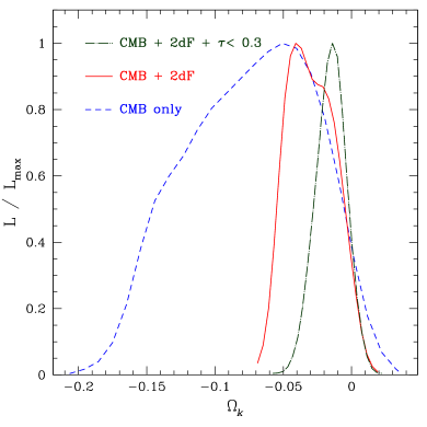
Figure 5: The one dimensional marginalized posterior likelihood for $\Omega_{k}$ for CMB data only (dashed line), CMB plus 2dFGRS $P(k)$ (solid line), and CMB plus 2dFGRS $P(k)$, with a prior on the optical depth of $\tau<0.3$ (dot-dashed line). Closed models have $\Omega_{k}<0$.

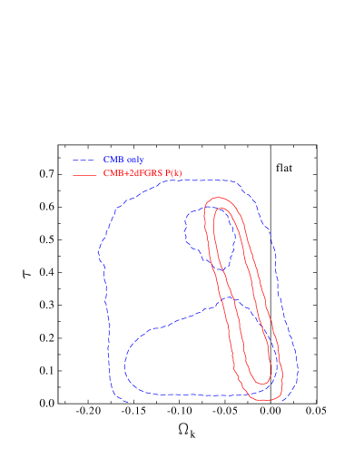
Figure 6: The marginalized posterior likelihood in the $\Omega_{k}-\tau$ plane for the basic-six plus $\Omega_{k}$ parameter set. The dashed lines show the 68% and 95% contours obtained in the CMB only case. The solid contours correspond to the constraints obtained in the CMB plus 2dFGRS $P(k)$ case.

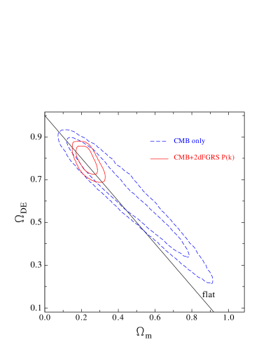
Figure 7: The marginalized posterior likelihood in the $\Omega_{\rm m}-\Omega_{\rm DE}$ plane for the basic-six plus $\Omega_{k}$ parameter set. The dashed lines show the 68% and 95% contours obtained in the CMB only case. The solid contours correspond to constraints in the CMB plus 2dFGRS $P(k)$ case.

There is a strong theoretical prejudice that we live in a flat universe with $\Omega_{k}=0$. The first detections of the acoustic peaks in the CMB temperature power spectrum, the location of which is a measure of the geometry of the universe, showed that the universe is close to being flat (de Bernardis et al. 2000). These results served to reinforce the prejudice that the curvature of the universe must be exactly zero – and it is true that, to date, no work has found any strong indication of a significant deviation from $\Omega_{k}=0$. However, as the flatness of the universe is one of the most important predictions of inflationary models, this assumption must be properly tested against new datasets. We must bear in mind, when comparing values reported for cosmological parameters, that many works simply assume $\Omega_{k}=0$. Other parameters, for example the scalar spectral index, are sensitive to the prior assumed for $\Omega_{k}$.

We plot the marginalized likelihood function for $\Omega_{k}$ in Fig. 5, for different datasets. The dashed curve shows the results for the CMB data alone, reminding us of the well-known (but frequently forgotten) result that the CMB data alone do not require a flat universe. Even though values of $\Omega_{k}>0$ (open models) are practically ruled out, a wide range of closed models is allowed, with the best fitting value given by $\Omega_{k}=-0.074_{-0.052\,(0.084)}^{+0.049\,(0.076)}$ at 68% (95%) confidence. The solid line in Fig. 5 shows how incorporating the 2dFGRS power spectrum helps to tighten the constraints on $\Omega_{k}$. The addition of power spectrum information helps to break the geometrical degeneracy between $\Omega_{\rm m}$ and $\Omega_{\rm DE}$ (see Fig. 7 and the final paragraph of this subsection). This is one of the most important effects of the incorporation of LSS information into the analysis. In the CMB plus 2dFGRS $P(k)$ case, we get $\Omega_{k}=-0.029^{+0.018\,(0.032)}_{-0.018\,(0.028)}$.

It is particularly important to note the effect that the prior on the optical depth to the last scattering surface, $\tau$, has on the inferred value of the curvature of the universe. Fig. 6 shows the constraints in the $\Omega_{k}-\tau$ plane. The addition of the 2dFGRS power spectrum shrinks the allowed region by tightening up the constraints on $\Omega_{k}$, but the resulting likelihood contours show a clear degeneracy between the two parameters, with the high values of $\tau$ preferring more negative values of $\Omega_{k}$. This degeneracy is responsible for the broad error bars on these parameters. If one adopts a restrictive prior on the optical depth of $\tau<0.3$, as recommended by the WMAP team based on the lack of a large signal in polarization autocorrelation, then the results for $\Omega_{k}$ are more in line with those in the literature, as shown by the dot-dashed line in Fig. 5. In this case we find $\Omega_{k}=-0.015_{-0.011\,(0.020)}^{+0.011\,(0.023)}$ for the combined CMB plus 2dFGRS datasets. We shall return to the issue of the choice of prior for the optical depth in Section 4.4.

Finally, we highlight the constraints on the densities of dark matter and dark energy obtained when the assumption of a flat universe is dropped. Fig. 7 shows the results for the case of CMB data alone (dashed lines) and for CMB data plus the 2dFGRS $P(k)$ (solid lines). As we have seen in several previous examples, there is a dramatic improvement in the quality of the constraints on these parameters once the galaxy clustering data is incorporated into the analysis. There is compelling evidence for a dark energy component in the universe.

3.5 Six parameters plus the dark energy equation of state

Over the past decade, mounting evidence has been presented for the accelerating expansion of the Universe, based on the interpretation of the Hubble diagram of Type-1a supernovae (Perlmutter et al. 1999; Riess et al 2004). Independent support for the presence of a dynamically dominant, negative pressure component in the energy-density budget of the Universe has also come from fitting cosmological models to CMB and LSS datasets (see Section 3.4 and Efstathiou et al. 2002). Although we can infer the presence of this component, dubbed dark energy, we know practically nothing about its nature. A plethora of theoretical models have been proposed for the dark energy (e.g. see the review by Sahni 2004). One of the key properties of the dark energy which can be used to pare down the market of possible models is the equation of state of the dark energy, that is the ratio of its pressure to density, $w_{\rm DE}$.

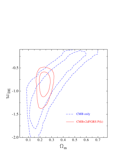
Figure 8: The marginalized posterior likelihood in the $\Omega_{\rm m}-w_{\rm DE}$ plane for the basic six plus $w_{\rm DE}$ parameter set. The dashed lines show the 68% and 95% contours obtained in the CMB only case. The solid contours show the corresponding constraints obtained in the CMB+2dFGRS $P(k)$ case.

Until now we have assumed that the dark energy component corresponds to the cosmological constant, with a fixed equation of state specified by $w_{\rm DE}=-1$. However, this is only one manifestation of the many possible forms that the dark energy could take. Any component with an equation of state $w_{\rm DE}<-1/3$ will result in an accelerating rate of expansion today. In this section, we explore dark energy models with a constant equation of state, allowing for variations in the redshift independent value of $w_{\rm DE}$. We also consider models with $w_{\rm DE}<-1$, sometimes referred to as ‘phantom energy’.

Fig. 8 shows the marginalized constraints in the $w_{\rm DE}-\Omega_{\rm m}$ plane. In the CMB only case, we find $w_{\rm DE}=-0.93_{-0.47}^{+0.49}$, consistent with a cosmological constant. When the 2dFGRS power spectrum is included in the analysis, the preferred value increases somewhat to $w_{\rm DE}=-0.85_{-0.17}^{+0.18}$. If we also include the supernova type Ia data from Riess et al. (2004), our result scarcely changes, with $w_{\rm DE}=-0.87_{-0.12}^{+0.12}$. Phantom energy models are permitted in the case of CMB data only, with the $95\%$ limit on the equation of state of $w_{\rm DE}>-1.66$. However, once the 2dFGRS $P(k)$ and supernovae type-Ia data are included, the allowed region shrinks to a smaller zone with $w_{\rm DE}>-1.19$ at $95\%$, showing that phantom energy models are disfavoured by the currently available data. These results show that the data prefers lower values of $w_{\rm DE}$ than suggested by previous work using the SDSS power spectrum (MacTavish et al. 2005). Our results are consistent with the dark energy taking the form of a cosmological constant. We will discuss this point further in Section 6.

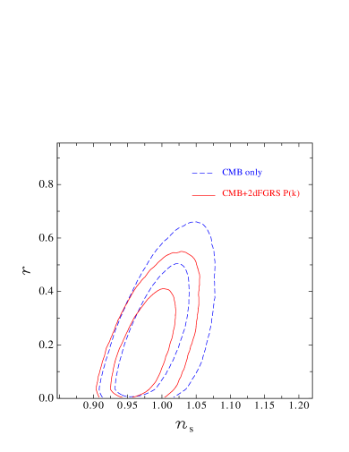
Figure 9: The marginalized posterior likelihood in the $n_{\rm s}-r$ plane for the basic-six plus $r$ parameter set. The dashed lines show the 68% and 95% contours obtained in the CMB only case. The solid contours show the corresponding results in the CMB plus 2dFGRS $P(k)$ case.

3.6 Six parameters plus non-zero tensor modes

We now add the ratio of the amplitude tensor to scalar perturbations, $r$, to the basic-six parameter set. This case is an important one to consider as tensor modes are predicted to be present in many inflationary models. Moreover, as we shall see, several cosmological parameters are degenerate with $r$ and in the literature tensor modes have often been ignored when presenting constraints on these parameters.

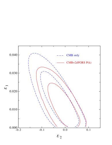
Figure 10: The marginalized posterior likelihood in the $\epsilon_{1}-\epsilon_{2}$ plane for the basic-six plus $r$ parameter set. The dashed lines show the 68% and 95% contours obtained in the CMB only case. The solid contours correspond to the results obtained in the CMB plus 2dFGRS $P(k)$ case.

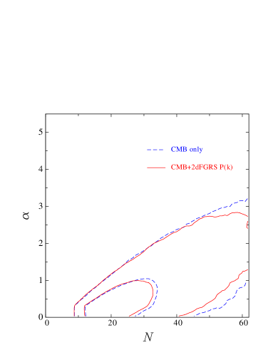
Figure 11: The marginalized posterior likelihood in the $\alpha-N$ plane for the basic-six plus $r$ parameter set. The dashed lines show the 68% and 95% contours obtained in the CMB only case. The solid contours show the results in the CMB plus 2dFGRS $P(k)$ case.

The constraints imposed on $r$ by CMB information alone are $r<0.52$ at $95\%$. Including the 2dFGRS $P(k)$ data reduces the importance of tensors slightly, yielding $r<0.41$ at $95\%$. Fig. 9 shows the two-dimensional marginalized likelihood contours in the $n_{\rm s}-r$ plane for the cases of CMB data only (dashed lines) and CMB plus the 2dFGRS $P(k)$ (solid lines). Tensor modes contribute to the CMB temperature power spectrum only on large angular scales, leading to a reduction in the scalar perturbations on these scales to match the observations. In order to maintain the amplitude of scalar perturbations on smaller angular scales, an increase in the scalar spectral index, $n_{\rm s}$, is required. This degeneracy results in a broader allowed range for $n_{\rm s}$ than in the case where only scalar modes are considered.

The constraints on $r$ and $n_{\rm s}$ can be translated into the horizon flow parameters, $\epsilon_{1}$ and $\epsilon_{2}$, using the relations given by Mukhanov et al. (1992):

$$1-n_{\rm s} = 2\epsilon_{1}+\epsilon_{2}$$ (16)

$$r = 16\epsilon_{1}.$$ (17)

The horizon flow parameters are related to derivatives of the Hubble parameter during inflation (Schwarz et al. 2001). Leach & Liddle (2003a) give equations relating the horizon flow parameters to the derivatives of the inflaton potential and discuss the motivation for the truncation of the slow-roll expansion after $\epsilon_{2}$. The constraints on the horizon flow parameters are shown in Fig. 10. The degeneracy between $r$ and $n_{s}$ translates into a degeneracy in $\epsilon_{1}$ and $\epsilon_{2}$.

If we restrict our attention to monomial inflation, i.e. potentials of the form $V\propto\phi^{\alpha}$, then the horizon flow parameters can be related to the power law index, $\alpha$, and the number of $e$-folds of inflation for the scale considered, $N$, by the simple relations (Leach & Liddle 2003b):

$$\epsilon_{2} = \frac{4\epsilon_{1}}{\alpha}$$ (18)

$$N = \frac{\alpha}{4}\left(\frac{1}{\epsilon_{1}}-1\right).$$ (19)

To obtain constraints on these new parameters, we have translated our results for $\epsilon_{1}$ and $\epsilon_{2}$ into the $\alpha-N$ plane. In doing so, we have restricted our attention to the region where $\epsilon_{2}>0$, following Liddle & Leach (2003b), who argue that this part of the horizon flow parameter space contains the most likely models in which inflation will end naturally with a violation of the slow-roll approximation. Our results are plotted in Fig. 11. We find that $\alpha<2.33$ at $95\%$ for CMB data alone and $\alpha<2.27$ (95%) for CMB plus the 2dFGRS $P(k)$. To obtain this result, we have followed Seljak et al. (2005) and take into account the maximum number of e-folds, $N_{\rm max}=60$, of slow-roll inflation experienced at the pivot scale $k=0.05\,\mathrm{{Mpc^{-1}}}$, thus further restricting the second horizon flow parameter, $\epsilon_{2}>0.0167$. (Note that Leach & Liddle 2003b use a different pivot scale to ours.) Our constraint on $\alpha$ implies that the $\lambda\phi^{4}$ inflation model is ruled out. This is the first time that the CMB data alone have been of sufficient quality to completely reject this model. Seljak et al. (2005) reached a similar conclusion using different datasets: the WMAP data, the SDSS galaxy power spectrum and either the power spectrum of the Ly-$\alpha$ forest or the amplitude of the matter power spectrum, as inferred from the bias of SDSS galaxies.

We now turn our attention to power-law inflationary models, in which the scale factor of the universe grows with time as $a\propto t^{p}$ with $p>1$. In such models, the horizon flow parameters are simply given by

$$\epsilon_{1} = \frac{1}{p}$$ (20)

$$\epsilon_{\rm i} = 0\,\,\,i\geq 2.$$ (21)

Substitution of these relations in Eq. 17 gives a relation between $n_{\rm s}$ and $r$:

$$r=8(1-n_{\rm s}).$$ (22)

To analyse this kind of model, we ran a new set of chains fixing the tensor to scalar ratio using Eq. 22. In this case we get $n_{s}=0.978^{+0.010}_{-0.010}$ for the CMB data alone and $n_{s}=0.9762^{+0.0094}_{-0.0092}$ in the CMB plus 2dFGRS case. The constraints on $r$ are also tighter, with $r<0.31$ at $95\%$. We note that the best fitting values for the horizon flow parameters of $\epsilon_{1}=0.0123^{+0.0080}_{-0.0082}$ (corresponding to $p=81^{+163}_{-32}$) and $\epsilon_{2}=-0.004^{+0.040}_{-0.040}$ are in complete agreement with the power law inflation picture.

4 The role of priors

It is often claimed that we have entered an era of precision cosmology, in which the values of the cosmological parameters are known with high accuracy. The CMB measurements alone go a long way towards realizing this ideal, but ultimately fall short due to the presence of well known degeneracies between the cosmological parameters (Efstathiou & Bond 1999). Some of these degeneracies can be broken with the incorporation of other information into the analysis (such as, for example, LSS, SN Ia or the power spectrum of the Ly-$\alpha$ forest). However, many degeneracies remain even after the addition of these datasets. Another way to break degeneracies is by imposing priors on parameters, which can have implications for the derived parameter constraints (see, for example, Bridle et al. 2003a). In this section we revisit the constraints obtained for the different parameter sets and priors and assess which of our results are the most robust.

4.1 The baryon density

One of the most important achievements of modern cosmology is the agreement between the value of the physical density of baryons determined from CMB data and that inferred from Big Bang Nucleosynthesis (BBN) arguments and distant quasar absorption spectra. In the present analysis, we obtain a value for the baryon density of $\omega_{\rm b}=0.0229^{+0.0012}_{-0.0013}$ from the CMB data alone that is consistent with the latest constraint from BBN: $\omega_{\rm b}=0.022\pm 0.002$ (Cuoco et al. 2004). This agreement is reinforced when the 2dFGRS $P(k)$ is added to the analysis, with $\omega_{\rm b}=0.0225^{+0.0010}_{-0.0010}$. The variation in the value of $\omega_{\rm b}$ obtained between the different parameter sets and priors that we have analysed is smaller than the 1$\sigma$ error bars, showing the robustness of this result. This level of agreement is all the more remarkable when one considers the quite different epochs to which the various datasets relate: BBN is a theory that describes processes occurring in the very early universe, just a few minutes after the Big Bang, while the CMB maps the universe as it was a few hundred thousand years after the Big Bang, and the galaxy power spectrum refers to the present day universe, over 13 billion years later. The fact that we can tell a coherent story over such a huge baseline in time and physical conditions provides an impressive verification of our cosmological model.

4.2 The dark matter density

A scan across the third rows of Tables 2 and 3 shows that the value of $\omega_{\rm dm}$ is largely insensitive to the priors applied to the other parameters. The one exception is when the flatness prior, $\Omega_{k}=0$, is relaxed, in which case we obtain a smaller value for $\omega_{\rm dm}$ with larger errors. The constraints obtained on $\omega_{\rm dm}$ in the CMB only and CMB plus 2dFGRS $P(k)$ cases are fully consistent.

The implications of the value of $\omega_{\rm dm}$ for the matter density $\Omega_{\rm m}$ do, however, depend on the priors implemented. In the basic-six plus $f_{\nu}$ parameter set, for the CMB plus 2dFGRS case we find $\Omega_{\rm m}=0.282\pm 0.040$, but it can be as low as $\Omega_{\rm m}=0.224\pm 0.022$ for the basic-six plus $r$ parameter set. With the exception of the case of non-zero neutrino mass, all our estimates of $\Omega_{\rm m}$ lie significantly below the standard choice of 0.3. Fig. 12 illustrates how the choice of parameter space affects the results obtained. The constraints in the $\Omega_{\rm m}-\sigma_{8}$ plane in the basic-six parameter set are tighter than those obtained when the neutrino fraction, $f_{\nu}$, is incorporated into the analysis; for the latter case, a bigger region with lower values of $\sigma_{8}$ is allowed by the data. A similar situation can be seen in Fig. 13 for the $\Omega_{\rm m}-h$ plane. The values of $h$ preferred by the data are lower when non-flat models are considered in the analysis. These discrepancies cause differences in the marginalized results obtained for these parameters. This situation occurs in many other cases and in general the influence of the parameter set is non-negligible. For this reason, constraints on a given parameter should always be quoted together with the parameter space explored in the analysis. Fig. 13 shows the 1$\sigma$ limits on the Hubble constant derived by the HST Key Project (Freedman et al. 2001). These constraints on $h$ are substantially broader than those obtained from the CMB plus 2dFGRS power spectrum, showing that including the Key Project measurement as a prior would have little impact on our results.

Figure 12: The marginalized posterior likelihood in the $\Omega_{\rm m}-\sigma_{8}$ plane obtained using CMB plus 2dFGRS information for different parameter sets. The solid lines correspond to the 68% and 95% contours obtained for the basic-six parameter set. The dashed lines correspond to the results obtained when the neutrino fraction $f_{\nu}$ is also allowed to vary. The dot-dashed lines show constraints from weak lensing measurements from Hoekstra et al. (2002).

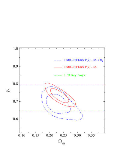
Figure 13: The marginalized posterior likelihood in the $\Omega_{\rm m}-h$ plane obtained using CMB plus 2dFGRS information for different parameter sets. The solid lines correspond to the 68% and 95% contours obtained for the basic-six parameter set. The dashed lines show the results obtained when non-flat models are considered (basic-six plus $\Omega_{k}$). The dot-dashed lines show the 1$\sigma$ constraint on $h$ from the HST Key Project (Freedman et al. 2001).

4.3 The amplitude of fluctuations

When constraining the values of the cosmological parameters, we only use information from the shape of the galaxy power spectrum and not from its amplitude. Therefore the constraints on the amplitude of density fluctuations come principally from the CMB data, with the LSS data playing an indirect role by tightening the constraints on parameters which yield degenerate predictions for the CMB. The recovered values of $\sigma_{8}$ range from $\sigma_{8}=0.678_{-0.072}^{+0.073}$ for the basic-six plus $f_{\nu}$ parameter space to $\sigma_{8}=0.817_{-0.079}^{+0.077}$ for non-flat models (basic-six plus $\Omega_{k}$). Adding more data sets, such as the X-ray cluster luminosity function, or other measurements of the amplitude of fluctuations may help to improve the constraint on $\sigma_{8}$, but the theoretical modelling of these observational datasets is less straightforward. In Fig. 12 we compare our results with constraints from measurements of weak lensing from Hoekstra et al. (2002). Henry (2004) used the temperature function of X-ray clusters to find $\sigma_{8}=0.66\pm{0.16}$, in good agreement with the basic-six plus neutrino mass fraction model. Similar constraints have been obtained by other groups (Bacon et al. 2003; Heymans et al. 2005).

4.4 The optical depth

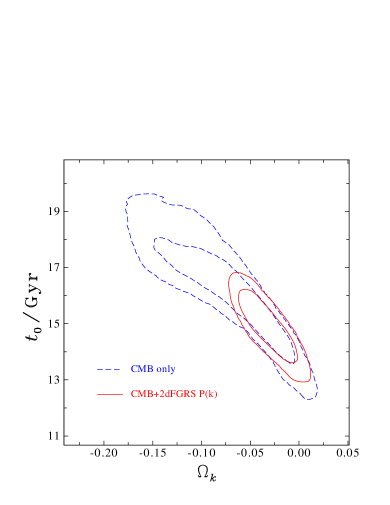
Figure 14: The marginalized posterior likelihood in the $\Omega_{k}-t_{0}$ plane for the basic-six plus $\Omega_{k}$ parameter set. The dashed lines show the 68% and 95% contours obtained in the CMB only case. The solid contours correspond to the constraints obtained in the CMB plus 2dFGRS case.

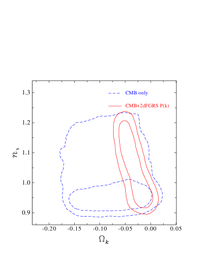
Figure 15: The marginalized posterior likelihood in the $\Omega_{k}-n_{\rm s}$ plane for the basic six plus $\Omega_{k}$ parameter set. The dashed lines show the 68% and 95% contours obtained in the CMB only case. The solid contours correspond to the constraints obtained in the CMB plus 2dFGRS case.

The optical depth to the last scattering surface has an important effect on nearly all other cosmological parameters. The signal for $\tau>0$ comes from the temperature-polarization cross-correlation on large angular scales. Intriguingly, Hansen et al. (2004) performed a temperature-polarization analysis of the first year WMAP data for the northern and southern hemispheres separately and found that, whereas the northern hemisphere points to $\tau=0$, the southern hemisphere prefers a value of $\tau=0.24_{-0.07}^{+0.06}$, inconsistent with $\tau=0$ at the 2$\sigma$ level, with the suggestion that the signal for $\tau>0$ may be due to foreground structures in the southern hemisphere.

In their analysis of the first year WMAP data Spergel et al. (2003) imposed a prior of $\tau<0.3$, justifying this by the need to avoid ‘unphysical’ regions of parameter space. In Section 3.4 we demonstrated, as previously pointed out by Tegmark et al. (2004b), the strong effect this prior has on our results. In particular, the $\tau<0.3$ prior is required to reconcile the constraints on $\Omega_{k}$ with the flatness prediction from inflation in the basic-six plus $\Omega_{k}$ parameter set, and to produce tight constraints on neutrino masses in the basic-six plus $f_{\nu}$ case. The situation should improve with the release of the second and subsequent years of data from WMAP, which will be able to produce improved polarization maps. In the meantime, the effect of this important prior must be borne in mind when interpreting the results from multi-parameter analyses.

4.5 The flatness prior

The prior of $\Omega_{k}=0$ is widely used when constraining cosmological parameters. It is important to remember that, if the assumption of flatness is relaxed, the preferred value is actually $\Omega_{k}<0$ and only marginally consistent with $\Omega_{k}=0$. The assumption of flatness has a major impact in the values of many cosmological parameters.

The value obtained for the age of the universe, $t_{0}$, shows an important change when $\Omega_{k}$ is allowed to float, and is only marginally consistent with the values found for $\Omega_{k}=0$. Fig. 14 shows the marginalized two-dimensional likelihood contours in the $\Omega_{k}-t_{0}$ plane. There is a clear degeneracy between these two parameters, with lower values of $\Omega_{k}$ preferring higher values of $t_{0}$; the incorporation of the 2dFGRS $P(k)$ data does not break this degeneracy completely. The same degeneracy can be seen in the $\Omega_{k}-h$ plane, which implies that a prior on the Hubble constant from the HST key project (Freedman et al. 2001) may improve the situation, but even then the constraints on these parameters are less robust than in the flat case.

The scalar spectral index, $n_{\rm s}$, also merits special attention. In Section 3.2, we pointed out that the constraint on $n_{\rm s}$ in the basic-six model is only marginally consistent with $n_{\rm s}=1$; this spectrum is formally excluded at the $95\%$ confidence level. Fig. 15 shows the marginalized two-dimensional likelihood contours in the $\Omega_{k}-n_{\rm s}$ plane. When CMB information alone is used, there is a wide allowed region that shrinks considerably when the 2dFGRS power spectrum is included. In the latter case, there is a correlation between the parameters which makes the constraints on $n_{\rm s}$ much broader than those obtained for the special case of $\Omega_{k}=0$. Taking into account that the evidence for $n_{\rm s}<1$ is weaker once more general parameter sets are considered (such as, for example, the basic-six plus $f_{\nu}$ set) and that the current data has a slight preference for closed models (even when the prior of $\tau<0.3$ is applied), we advocate caution before claiming a detection of a significant deviation from scale invariance.

4.6 Tensor modes

Another commonly applied prior is the assumption that tensor modes can be neglected. It is important to include the amplitude of tensor modes as a free parameter, not only because this has strong implications for inflationary models, but also because many other parameters are degenerate with the amplitude of tensors, resulting in the growth of the allowed regions for these parameters. The parameters that are most strongly influenced by the assumption about tensor modes are $n_{\rm s}$, $\Omega_{\rm m}$ and $h$.

5 Beyond the simplest model

5.1 How many parameters should float?

We have shown that a model in which five parameters are allowed to vary gives a good description of the CMB and LSS datasets. We then went on to explore six and seven parameter sets, finding that, in some cases, the results obtained for certain parameters depended upon the choice of parameters varied. But are we justified in adding extra free parameters to our basic-five set?

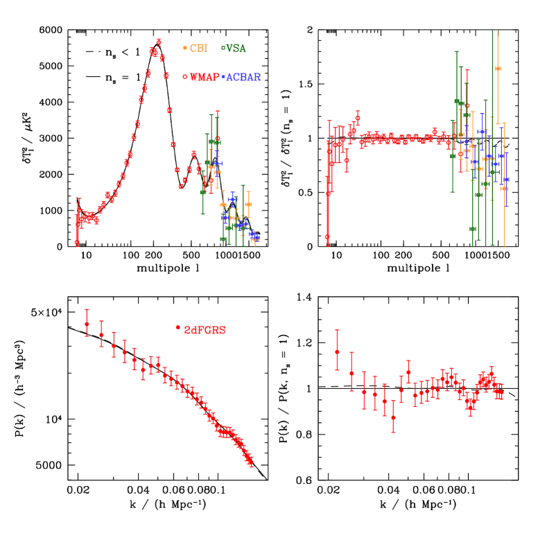
Figure 16: Model fits to the CMB datasets (top panels) and 2dFGRS $P(k)$ (bottom panels) in the cases of the basic-five (solid line) and basic-six (dashed line) models, with the best fitting parameter values listed in Table 3. The model $P(k)$ have been convolved with the window function of the 2dFGRS from Cole et al. (2005). In the right-hand panels, the model curves and datapoints have been divided by the best fitting basic-five model to expand the y-axis.

The simplest way to make an objective assessment of different models is to establish whether or not they afford a better description of the data, which is usually done by computing likelihood ratios. However, it is important to compensate for the fact that adding extra parameters should necessarily improve the fit to the data. Liddle (2004) has advocated the use of two simple statistics that quantify the level of improvement in the description of cosmological datasets as new free parameters are added to the theoretical models. These statistics allow us to ascertain whether the addition of a new parameter is justified, i.e. does it produce a better than expected enhancement in the accuracy with which the data is reproduced? The statistics, the Akaike Information Criterion (AIC; Akaike 1974) and the Bayesian Information Criterion (BIC; Schwarz 1978) have a long track record of application in other branches of physics, but have largely been ignored in cosmology. The definitions of the two statistics are straightforward:

$${\tt AIC} = -2\ln(\mathcal{L})+2N_{\rm par},$$ (23)

$${\tt BIC} = -2\ln(\mathcal{L})+N_{\rm par}\ln(N_{\rm data}),$$ (24)

where $\mathcal{L}$ is the maximum likelihood, $N_{\rm par}$ is the number of parameters varied in the model and $N_{\rm data}$ is the number of datapoints included in the analysis. The model that best describes the data with the most economical use of parameters is the one that minimizes these quantities. In both expressions, the first term favours models which provide better fits to the data, while the second penalizes large numbers of parameters. We note that, as the value of $\ln(N_{\rm data})>2$ in our analysis, the BIC actually gives a higher penalty to the number of free parameters than is the case for the AIC.

Table 4: The number of parameters, the likelihood and the values of the AIC and BIC statistics for the various models analysed in this paper. In all cases, $N_{\rm data}=1403$.

Model	$N_{\rm par}$	$-2\ln(\mathcal{L})$	AIC	BIC
b5	5	1495.8	1505.8	1532.1
b6	6	1492.1	1504.1	1535.6
b6 + $f_{\nu}$	7	1491.3	1505.3	1542.0
b6 + $\Omega_{k}$	7	1490.4	1504.4	1541.1
b6 + $w_{\rm DE}$	7	1491.5	1505.5	1542.2
b6 + $r$	7	1491.7	1505.7	1542.4

Table 4 provides a summary of the number of parameters, the likelihood and the values of the AIC and BIC statistics for the models considered in this paper. The addition of extra free parameters does of course lead to an increase in the likelihood of the description of the data by the model. The message conveyed by the value of the AIC statistic is less clear. All models show a slight decrease in the value of the AIC statistic compared with the basic-five set, but the BIC statistic paints a quite different picture. Liddle reports that a difference in the BIC of 2 should be regarded as ‘positive evidence’ and of 6 as ‘strong evidence’ in favour of the model with the smaller value of BIC. Therefore, there is apparently ‘positive evidence’ that we should not expand the basic-five model to allow the scalar spectral index to float and ‘strong evidence’ that we really should not have burdened the reader with the basic-six plus one more free parameter models.

This conclusion, and indeed the basic BIC formula itself, appears to disagree with the approach of this paper. For data with Gaussian errors, the addition of a further parameter would be expected to reduce $-2\ln{\cal L}$ by one via the usual ‘degree of freedom’ rule (although note that this strictly applies only to parameters linearly related to the data, such as polynomial expansion coefficients). Furthermore, the reduction in $-2\ln{\cal L}$ should be distributed as $\chi^{2}$ with 1 degree of freedom if the new parameter is not part of the true model, independent of the number of data points. A reduction in $-2\ln{\cal L}$ of 4 therefore amounts to rejection at 95% confidence of the hypothesis that a new parameter is not required. Thus, the fact that allowing deviations from scale invariance reduces $-2\ln{\cal L}$ by 3.7 amounts to marginal evidence for the reality of tilt. This reasoning matches the AIC approach quite well, as long as the coefficient 2 in the $2N_{\rm par}$ term is regarded as being adjustable according to the significance level of interest.

The BIC statistic is an approximate form of the ‘Bayesian evidence’ (Hobson, Bridle & Lahav 2002, Liddle 2004, Trotta 2005). One of the conditions that must be satisfied in order for the BIC to be a good approximation to the Bayesian evidence is the independence of the data points under consideration. By setting $N_{\rm data}=1403$ in the definition of the BIC in Eq. 24, we are effectively treating all of the data points used in our analysis as independent. Our calculation of the BIC therefore gives an overly pessimistic impression of the impact of adding of new parameters. If, for example, an eigenmode analysis or ‘radical’ data compression technique was applied to the full set of CMB data points used in our analysis, this would produce a much smaller set of genuinely independent data points which fully describe the CMB measurements (Bond, Jaffe & Knox 2000). The values of the AIC and BIC statistics would become closer if recomputed for this ‘reduced’ set of datapoints. One might argue that one should compute the Bayesian evidence rather than approximations such as the BIC. There are two reasons why we have not done this. Firstly, the Bayesian evidence is hard to compute accurately using MCMC techniques, although fast algorithms are under development (Mukherjee, Parkinson & Liddle 2005). Secondly, the definition of the prior on a parameter is part of the model tested in the Bayesian evidence approach and we believe that this is a weak point in the method for the following reason. Since the choice of prior is arbitrary to some extent, it is possible in principle to select a prior such that the Bayesian evidence increases upon the addition of new parameters. We prefer the effectively frequentist argument of simply requiring a reduction in $-2\ln{\cal L}$ of order unity in order to claim the detection of another degree of freedom.

5.2 Details of the evidence for tilt

Putting aside the caveat raised by the BIC statistic, it is important to look at the basic-five and basic-six model results for the scalar spectral index in more detail, as they have important implications for inflationary models. To recap, in Section 3.2 we set $n_{\rm s}=1$, i.e. the scale invariant value of the spectral index for primordial scalar fluctuations. In Section 3.3, we treated the spectral index as a free parameter and found that $n_{\rm s}=1$ was on the $95\%$ limit. Fig. 16 shows the best fitting models to the CMB temperature power spectrum data (upper panels) and the 2dFGRS $P(k)$ (lower panels) for the basic-five (solid lines) and basic-six (dashed lines) models. The difference between the two models is small and comes mostly from scales beyond those probed by WMAP; this is quantified in the right-hand panels in which the models and datapoints have been divided by the $n_{\rm s}=1$ model. Fig. 17 shows the likelihood quotients between the basic-five and basic-six models for each dataset separately. It is clear that the datasets primarily responsible for driving the scalar spectral index away from the scale invariant value are the CBI measurements and the 2dFGRS $P(k)$: the basic-six model represents only a modest improvement over the basic-five model in its description of the WMAP and VSA datasets, while the addition of an extra parameter makes very little difference to how well the ACBAR results are reproduced. Nevertheless, there is an impressive consistency between the various datasets: a systematic error in a single one of these might have resulted in an improved overall likelihood on the introduction of tilt, but at the price of a poorer fit to some of the correct datasets. This is not what we see: addition of the 2dFGRS strengthens a weak trend already present in the CMB data. Even so, the overall result remains tantalisingly placed in terms of its statistical significance: 95% confidence is not sufficient to claim firm detection of an effect of this importance. The best that can be said is that even a modest amount of extra data could easily move things into the territory of firm detection. The largest predicted deviations from $n_{\rm s}=1$ occur around the third CMB peak, at $\ell\simeq 800$, and the data here may be expected to improve rapidly.

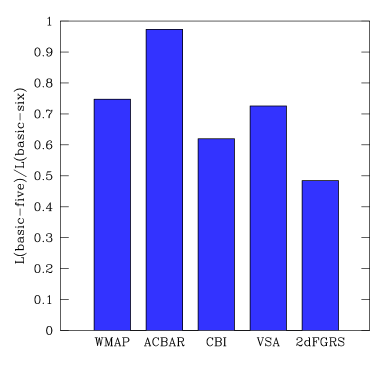
Figure 17: The likelihood ratios of the basic-five model to the basic-six model plotted in Fig.16 for the individual datasets used in our analysis.

6 Comparison with constraints obtained using the CMB data and the SDSS power spectrum

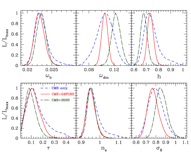
Figure 18: The marginalized one-dimensional posterior likelihood in the basic-six parameter space obtained for CMB information only (dashed lines), CMB plus the 2dFGRS $P(k)$ (solid lines) and CMB plus the SDSS (dot-dashed lines).

Table 5: The marginalized 68% interval constraints (unless otherwise stated) on cosmological parameters obtained using CMB data and the SDSS galaxy power spectrum for different parameter sets.

	b5	b6	b6 + $f_{\nu}$	b6 + $\Omega_{k}$	b6 + $w_{\rm DE}$	b6 + $r$
$\Omega_{k}$	0	0	0	$-0.070^{+0.037}_{-0.039}$	0	0
$\Theta$	$1.0493^{+0.0036}_{-0.0036}$	$1.0436^{+0.0048}_{-0.0047}$	$1.0436^{+0.0047}_{-0.0048}$	$1.0408^{+0.0051}_{-0.0052}$	$1.0440^{+0.0048}_{-0.0049}$	$1.0452^{+0.0047}_{-0.0047}$
$\omega_{dm}$	$0.1227^{+0.0074}_{-0.0073}$	$0.1234^{+0.0070}_{-0.0071}$	$0.1304^{+0.0094}_{-0.0094}$	$0.106^{+0.010}_{-0.010}$	$0.104^{+0.012}_{-0.012}$	$0.1203^{+0.0069}_{-0.0069}$
$\omega_{b}$	$0.0242^{+0.0006}_{-0.0006}$	$0.0228^{+0.0009}_{-0.0009}$	$0.0225^{+0.0009}_{-0.0009}$	$0.0224^{+0.0011}_{-0.0012}$	$0.0235^{+0.0013}_{-0.0013}$	$0.0234^{+0.0010}_{-0.0010}$
$f_{\nu}$	0	0	$<0.104$ (95%)	0	0	0
$\tau$	$0.173^{+0.034}_{-0.036}$	$0.097^{+0.046}_{-0.045}$	$0.098^{+0.043}_{-0.044}$	$0.147^{+0.071}_{-0.077}$	$0.124^{+0.065}_{-0.064}$	$0.099^{+0.046}_{-0.046}$
$w_{\rm DE}$	$-1$	$-1$	$-1$	$-1$	$-0.45^{+0.23}_{-0.23}$	$-1$
$n_{s}$	1	$0.956^{+0.020}_{-0.020}$	$0.947^{+0.022}_{-0.022}$	$0.958^{+0.026}_{-0.032}$	$0.988^{+0.040}_{-0.039}$	$0.974^{+0.024}_{-0.025}$
$\log_{10}(10^{10}A_{s})$	$3.273^{+0.057}_{-0.061}$	$3.100^{+0.098}_{-0.098}$	$3.097^{+0.094}_{-0.095}$	$3.12^{+0.14}_{-0.15}$	$3.10^{+0.13}_{-0.13}$	$3.100^{+0.097}_{-0.098}$
$r$	0	0	0	0	0	$<0.31$ (95%)
$\Omega_{\rm DE}$	$0.710^{+0.030}_{-0.030}$	$0.682^{+0.035}_{-0.035}$	$0.603^{+0.070}_{-0.073}$	$0.577^{+0.083}_{-0.088}$	$0.557^{+0.085}_{-0.085}$	$0.706^{+0.034}_{-0.034}$
$t_{0}/{\rm Gyr}$	$13.35^{+0.12}_{-0.12}$	$13.65^{+0.20}_{-0.20}$	$13.97^{+0.26}_{-0.27}$	$16.2^{+1.2}_{-1.1}$	$14.35^{+0.56}_{-0.50}$	$13.54^{+0.21}_{-0.21}$
$\Omega_{\rm m}$	$0.289^{+0.030}_{-0.030}$	$0.317^{+0.035}_{-0.035}$	$0.397^{+0.073}_{-0.070}$	$0.49^{+0.12}_{-0.11}$	$0.443^{+0.084}_{-0.085}$	$0.294^{+0.034}_{-0.034}$
$\sigma_{8}$	$0.947^{+0.039}_{-0.040}$	$0.858^{+0.054}_{-0.054}$	$0.732^{+0.084}_{-0.083}$	$0.773^{+0.071}_{-0.071}$	$0.57^{+0.15}_{-0.16}$	$0.853^{+0.055}_{-0.055}$
$z_{re}$	$17.5^{+2.3}_{-2.4}$	$11.9^{+3.9}_{-3.9}$	$12.2^{+3.8}_{-3.9}$	$14.8^{+7.1}_{-7.1}$	$13.4^{+4.7}_{-4.9}$	$11.8^{+3.8}_{-3.9}$
$h$	$0.714^{+0.021}_{-0.021}$	$0.681^{+0.026}_{-0.026}$	$0.626^{+0.040}_{-0.042}$	$0.519^{+0.064}_{-0.067}$	$0.544^{+0.047}_{-0.047}$	$0.701^{+0.028}_{-0.029}$
$\sum{m_{\nu}}/\rm{eV}$	0	0	$<1.27$ (95%)	0	0	0

In this section, we replace the 2dFGRS $P(k)$ measured by Cole et al. (2005) with the power spectrum of SDSS galaxies estimated by Tegmark et al. (2004a) and examine the impact that this change has upon the values of the recovered cosmological parameters. There are a number of differences between the two measurements of the galaxy power spectrum. Firstly, the SDSS is a red-selected survey, while the 2dFGRS is blue-selected. Secondly, Tegmark et al. used a sophisticated eigenmode deconvolution apparatus to attempt to remove the effects of the survey window and redshift-space distortions; in contrast, Cole et al. used a simpler Fourier approach that compares to window-convolved models and quantifies redshift-space effects directly by comparison with realistic simulations.

Tegmark et al. (2004b) used the WMAP first year data and the SDSS galaxy power spectrum to constrain cosmological parameters. These authors modelled the galaxy power spectrum with a non-linear model for the matter fluctuations multiplied by a scale independent bias factor. The power spectrum data were used on scales larger than $k<0.20\,h\,\mathrm{{Mpc^{-1}}}$. It is not clear that a constant bias is a good approximation on scales for which the density fluctuations have become non-linear. We adopt a simpler approach and assume that the galaxy power spectrum can be related to the linear perturbation theory power spectrum of the mass through a constant shift in amplitude. As discussed earlier, the simulations used by Cole et al. indicate that redshift-space effects and other nonlinearities are unimportant for the 2dFGRS to our imposed limit of $k_{\rm max}=0.15\,h\,{\rm Mpc}^{-1}$.

We repeat the study of parameter space previously carried out using the CMB data plus the 2dFGRS $P(k)$ and present our results using the SDSS $P(k)$ instead in Table 5. For the most part, the results obtained with the SDSS $P(k)$ are compatible with those found using the 2dFGRS $P(k)$. There are, however, some cases in which the results are quite different. This point is illustrated using the results of the basic-six model in Fig. 18. In this plot, we compare the parameter constraints obtained using CMB data alone (dashed line) with the results for CMB data plus the 2dFGRS $P(k)$ (solid line) and for CMB data plus the SDSS $P(k)$ (dot-dashed line). For three out of the six parameters presented, $\omega_{\rm b}$, $\tau$ and $n_{\rm s}$, there is impressive agreement between the sets of results; the peaks in the likelihood distributions coincide in the CMB only and CMB plus $P(k)$ cases, and the results are consistent to better than the 68% confidence intervals. The agreement between the sets of results for the scalar spectral index in particular is excellent. However, for the other three parameters plotted, $\omega_{\rm dm}$, $h$ and $\sigma_{8}$, the agreement is less impressive; the differences in the recovered values of $h$ and $\sigma_{8}$ are driven by the change in $\omega_{\rm dm}$. The peak in the likelihood distributions for the CMB only and CMB plus 2dFGRS $P(k)$ cases are in good agreement, as remarked upon in Section 3. There is a clear discrepancy, however, with the preferred parameter values when using CMB data plus the SDSS $P(k)$. This is most marked for the physical density of dark matter, $\omega_{\rm dm}$. Cole et al. (2005) noted that the SDSS $P(k)$ has a slightly bluer slope than that of the 2dFGRS, favouring higher values of $\Omega_{\rm m}$.

There are two other notable discrepancies between the results obtained with the SDSS and 2dFGRS $P(k)$ in our basic-six plus one additional free parameter models. When the assumption of a flat universe is relaxed, we find that the constraints on $\Omega_{k}$ are weaker in the SDSS case, $\Omega_{k}=-0.070_{-0.039(0.079)}^{+0.037(0.058)}$; the allowed range is nearly twice as broad as in the case of the 2dFGRS $P(k)$. This is because on the scales used in our analysis, the SDSS power spectrum does a poorer job of constraining $\Omega_{\rm m}$ compared with the 2dFGRS $P(k)$, and hence is not as effective at breaking the geometrical degeneracy. In the basic-six plus dark energy equation of state parameter set, we find $w_{\rm DE}=-0.45_{-0.23}^{+0.23}$ using the SDSS $P(k)$, much higher than we found in the case of the 2dFGRS $P(k)$ and inconsistent with a cosmological constant. If we also include the SNIa data from Riess et al. (2004), then we obtain a value for the equation of state that is consistent with our previous results: $w_{\rm DE}=-0.89_{-0.18}^{+0.19}$. Again, the discrepancy in the result for the equation of state can be traced back to the preferred values of $\omega_{\rm dm}$. We note that MacTavish et al. (2005) find similar results to ours for the equation of state of the dark energy using the SDSS galaxy power spectrum. Fig. 8 shows the degeneracy in the $\Omega_{\rm m}-w_{\rm DE}$ plane for CMB data alone. Adding information from the galaxy power spectrum breaks this degeneracy. If the galaxy $P(k)$ data prefer a high value of $\Omega_{\rm m}$, as is the case for the SDSS data, then a high value of $w_{\rm DE}$ will result.

It may be that these differences between 2dFGRS and SDSS amount to no more than an unlucky amount of cosmic variance, but clearly it would be more reassuring if the results showed greater consistency. It will therefore be important to see each dataset subjected to analysis by a variety of algorithms and codes, as happened following the Percival et al. (2001) 2dFGRS power-spectrum analysis (Tegmark, Zaldarriaga & Hamilton 2001). This older comparison found consistent results, but the comparison will now be more demanding, given the smaller errors arising from current datasets.

7 Summary

We have placed new constraints on the values of the basic cosmological parameters, using an up-to-date compilation of CMB data and the galaxy power spectrum measured from the final 2dFGRS by Cole et al. (2005). We have carried out a comprehensive exploration of parameter space, considering five, six and seven parameter models, making different assumptions about the priors used for certain parameters.

Our main results can be summarized as follows:

• A model in which five parameters are allowed to vary does a remarkably good job of describing the currently available CMB and LSS data.

• There is an impressive level of agreement between the results obtained for CMB data alone and for CMB data plus the 2dFGRS power spectrum data. If the 2dFGRS $P(k)$ is replaced by the SDSS $P(k)$, there is some tension between the parameter values preferred by the CMB and SDSS datasets.

• For some parameters, for example the physical density of dark matter, Hubble’s constant and the amplitude of density fluctuations, there is a significant tightening of the allowed range of parameter space when the 2dFGRS $P(k)$ is included in the analysis. In particular, we infer a density significantly below $\Omega_{\rm m}=0.3$.

• We find some evidence for a departure from a scale invariant primordial spectrum of scalar fluctuations. Our results for the scalar perturbation spectral index are only marginally consistent with the scale invariant value $n_{\rm s}=1$; this spectrum is formally excluded at the $95\%$ confidence level. However, this conclusion is weakened if we drop the assumption that the universe is flat or allow neutrinos to have a mass.

• We place new limits on the mass fraction of massive neutrinos: $f_{\nu}<0.105$ and $\sum m_{\nu}<1.2$ eV at the 95% level.

• Several parameters are sensitive to the choice of prior for the optical depth to the last scattering surface, $\tau$.

• We find that a wide range of closed universes are consistent with the CMB data. This range is restricted if we also consider the 2dFGRS $P(k)$ data. If we further assume a prior of $\tau<0.3$, then the preferred spatial curvature is close to flat.

• We confirm the evidence previously reported by Efstathiou et al. (2002) for a non-zero dark energy contribution to the energy-density of the universe.

• We find a redshift-independent equation of state for the dark energy of $w_{\rm DE}=-0.85_{-0.17}^{+0.18}$, consistent with a cosmological constant.

• Inflationary models with a scalar field potential with a $V(\phi)\propto\phi^{4}$ term are ruled out by our analysis.

The final message of this analysis is that meaningful comparison of the parameter constraints from different studies requires a clear listing of the free parameters and their prior distributions. Although current datasets measure many parameter combinations extremely well, important degeneracies remain. As we have discussed, there is a good chance that current measurements may be poised on the brink of rejecting the simplest 5-parameter model in favour of something more complicated. However, even if this step is taken, it will require much work before any such deviation from the standard model could have a unique interpretation.

References

Abazajian K. et al., 2005, AJ, 129, 1755

Ahmad Q.R., Allen R.C., Andersen T.C., 2001, Phys. Rev. Letters, 87, 071301

Allen S.W., Schmidt R.W., Bridle S.L., 2003, MNRAS, 346, 593

Akaike H., 1074, IEEE Trans. Auto. Control, 19, 716

Bacon D.J., Massey R.J., Refregier A.R., Ellis R.S., 2003, MNRAS, 344, 673

Barger V., Marfatia D., Whisnant K., 2003, Int. J. Mod. Phys., E12, 569

Bennett C.L., et al. , 2003, ApJS, 148, 1

de Bernardis P., et al., 2000, Nature, 404, 955

Bond J.R., Jaffe A.H., Knox, L., 2000, ApJ, 533, 19

Bridle S.L., Lahav O., Ostriker J.P., Steinhardt P.J., 2003a, Science, 299, 1532

Bridle S.L., Lewis A.M., Weller J., Efstathiou G., 2003b, MNRAS, 342, L72.

Cole S., et al. 2005, MNRAS, 362, 505

Colless M., et al., 2001, MNRAS, 328, 1039

Colless M., et al., 2003, astro-ph/0306581

Cuoco A., Iocco F., Magnano G., Miele G., Pisanti O., Serpico P.D., 2004, Int. J. Mod. Phys., A19, 4431

Croft R.A.C., Weinberg D.H., Bolte M., Burles S., Hernquist L. Katz N., Kirkman D., Tytler D., 2002, ApJ, 581, 20

de Oliveira-Costa A., Tegmark M., Zaldarriaga M., Hamilton A., 2004, Phys. Rev. D., 69, 063516

Dickinson C., et al. , 2004, MNRAS, 353, 732

Efstathiou G., 2003, MNRAS, 343, L95

Efstathiou G., 2004, MNRAS, 348, 885

Efstathiou G., Bond J.R., 1999, MNRAS, 304, 75

Efstathiou G., et al. 2002, MNRAS, 330, L29

Elgaroy O., et al., 2002, Phys. Rev. Letters, 89, 061301

Freedman W.L., et al., 2001, ApJ, 553, 47

Frenk C.S., White S.D.M., Davis M., 1983, ApJ, 271, 417

Gaztañaga E., Wagg J., Multamaki T., Montana A., Hughes D.H., 2003, MNRAS, 346, 47

Gaztañaga E., Norberg P., Baugh C.M., Croton D.J., 2005, MNRAS, 364, 620

Gelman A., Rubin D., 1992, Statistical Science, 7, 457

Gnedin N.Y., Hamilton A.J.S., 2002, MNRAS, 334, 107.

Hanany S., et al., 2000, 545, L5.

Hannestad S., 2002, Phys. Rev. D., 66, 125011

Hansen F.K., Balbi A., Banday A.J., Gorski K.M., 2004, MNRAS, 354, 905

Henry J.P., 2004, ApJ, 609, 603

Heymans C. et al., 2005, MNRAS, 361, 160

Hinshaw G., et al., 2003, ApJS, 148, 135

Hobson M.P., Bridle S.L., Lahav O., 2002, MNRAS, 335, 377

Hoekstra H., Yee H.K., Gladders M.D., 2002, ApJ, 577, 595

Hu W., Eisenstein D.J., Tegmark M., 1998, Phys. Rev. Letters, 80, 5255

Kogut A., et al., 2003, ApJS, 148, 161

Komatsu E., et al. 2003, ApJS, 148, 119

Kosowsky A., Milosavljevic M., Jimenez R., 2002, Phys. Rev. D., 66, 063007

Kuo C.L., et al., 2004, ApJ, 600, 32

Leach S.M., Liddle A.R., 2003a, MNRAS, 341, 1151

Leach S.M., Liddle A.R., 2003b, Phys. Rev. D., 68, 123508

Lewis A., Bridle S., 2002, Phys. Rev. D, 66, 103511

Lewis A., Challinor A., Lasenby A., 2000, Apj 538, 473

Liddle A.R., 2004, MNRAS, 351, L49

MacTavish C.J. et al., 2005, ApJ submitted, astro-ph/0507503

McDonald P., Seljak U., Cen R., Bode P., Ostriker J.P., 2005, MNRAS, 360, 147.

Metropolis N., Rosenbluth A., Rosenbluth R., Teller A., Teller E., 1953, J. Chem. Phys., 21, 1087

Mukhanov V.J., Feldman H.A., Brandenberger R.H., 1992, Phys. Rep., 215, 203

Mukherjee P, Parkinson D, Liddle A.R., 2005, MNRAS, submitted. (astro-ph/0508461)

Percival W.J., et al., 2001, MNRAS, 327, 1297

Percival W.J., et al., 2002, MNRAS, 337, 1068

Percival W.J., et al., 2004, MNRAS, 353, 1201

Perlmutter S., et al., 1999, ApJ, 517, 565

Peiris H.V., et al., 2003, ApJS, 148, 213

Pope A.C. et al., ApJ, 607, 655

Readhead A.C.S. et al., 2004, ApJ, 609, 498

Riess A.G., et al., 2004, ApJ, 607, 665

Sahni V., 2005, in Papantonopoulos E. ed., The Physics of the Early Universe. Springer, Berlin, p. 141

Schwarz D. J., Terrero-Escalante C. A., Garcia A. A., 2001, Phys. Let. B., 517, 243

Schwartz G., 1978, Annals of Statistics, 5, 461

Seljak U. et al., 2005, Phys. Rev. D, 71, 103515

Slosar A., Seljak U., Makarov A., 2003, Phys. Rev. D., 69, 123003

Spergel D.N., et al., 2003, ApJS, 148, 175

Tegmark M., Zaldarriaga M., Hamilton A.J.S., 2001, MNRAS,335, 887

Tegmark M. et al., 2004a, ApJ 606, 702

Tegmark M. et al., 2004b, Phys. Rev. D, 69, 103501

Trotta R, 2005, MNRAS, submitted. (astro-ph/0504022)

Verde L., et al., 2002, MNRAS, 335, 432

Verde L., et al., 2003, ApJS, 148, 195

Weinheimer C., 2003, Nucl. Phys. B (Proc. Suppl.), 118, 279

York D., et al., 2000, AJ, 120, 1579