A FUSE SURVEY OF INTERSTELLAR MOLECULAR HYDROGEN TOWARD HIGH-LATITUDE AGN

Abstract

We report results from a Far Ultraviolet Spectroscopic Explorer (FUSE) survey of interstellar molecular hydrogen (H₂) along 45 sight lines to AGN at high Galactic latitudes ($|b|>20^{\circ}$). Most (39 of 45) of the sight lines show detectable Galactic H₂ absorption from Lyman and Werner bands between 1000 and 1126 Å, with column densities ranging from N_H2 $=10^{14.17-19.82}$ cm^-2. In the northern Galactic hemisphere, we identify many regions of low N_H2 ($\leq 10^{15}$ cm^-2) between $\ell=60^{\circ}-180^{\circ}$ and at $b>54^{\circ}$. These “H₂ holes” provide valuable, uncontaminated sight lines for extragalactic UV spectroscopy, and a few may be related to the “Northern Chimney” (low Na I absorption) and “Lockman Hole” (low N_HI). A comparison of high-latitude H₂ with 139 OB-star sight lines surveyed in the Galactic disk suggests that high-latitude and disk H₂ clouds may have different rates of heating, cooling, and UV excitation. For rotational states $J=0$ and 1, the mean excitation temperature at high latitude, $\langle T_{01}^{\rm hl}\rangle=124\pm 8$ K, is somewhat higher than in the Galactic disk, $\langle T_{01}^{\rm disk}\rangle=86\pm 20$ K. For $J\geq 2$, the mean $\langle T_{\rm exc}\rangle=498\pm 28$ K, and the column-density ratios, N(3)/N(1), N(4)/N(0), and N(4)/N(2), indicate a comparable degree of UV excitation in the disk and low halo for sight lines with N_H2 $\geq 10^{18}$ cm^-2. The distribution of molecular fractions at high latitude shows a transition at lower total hydrogen column density (log N${}_{\rm H}^{\rm hl}\approx 20.38\pm 0.13$) than in the Galactic disk (log N${}_{\rm H}^{\rm disk}\approx 20.7$). If the UV radiation fields are similar in disk and low halo, this suggests an enhanced H₂ (dust-catalyzed) formation rate in higher-density, compressed clouds, which could be detectable as high-latitude, sheetlike infrared cirrus.

1 INTRODUCTION

Molecular hydrogen (H₂) is the most abundant molecule in the universe, comprising the majority of mass in interstellar molecular clouds that eventually form stars. In the diffuse interstellar medium, with visual extinctions $A_{V}\leq 1$ mag, the absorbing clouds exhibit detectable H₂ lines with molecular fractions, $f_{\rm H2}$, ranging from $10^{-6}$ at low H I column density up to $\sim$40% (Savage et al. 1977; Spitzer & Jenkins 1975; Shull et al. 2005). In sight lines with even greater extinction, the so-called translucent sight lines with $A_{V}=1-5$ mag (van Dishoeck & Black 1986), the molecular fraction can be as high as 70% (Rachford et al. 2002). Even though H₂ plays an important role in interstellar chemistry, many questions remain about its distribution, formation, and destruction in protostellar clouds. With the 1999 launch of the Far Ultraviolet Spectroscopic Explorer (FUSE) satellite, astronomers regained access to far ultraviolet (FUV) wavelengths below 1126 Å, needed to study H₂ via resonance absorption lines from its ground electronic state, X ${}^{1}\Sigma^{+}_{g}$, to the excited states, B ${}^{1}\Sigma_{u}^{+}$ (Lyman bands) and C ${}^{1}\Pi_{u}$ (Werner bands). In absorption by the cold clouds, the observed transitions originate in the ground ($v=0$) vibrational state from a range of rotational states, primarily $J=0$ (para-H₂ with total nuclear spin $S=0$) and $J=1$ (ortho-H₂ with nuclear spin $S=1$). Weaker absorption lines from excited states, $J\geq 2$, are also detected, which are produced by UV fluorescence and cascade following photoabsorption in the Lyman and Werner bands; see reviews by Spitzer & Jenkins (1975) and Shull & Beckwith (1982).

From the FUSE mission inception, H₂ studies have been an integral part of the science plan. The FUSE satellite, its mission, and its on-orbit performance are described in Moos et al. (2000) and Sahnow et al. (2000). The initial FUSE studies of H₂ appeared among the Early Release Observations (Shull et al. 2000; Snow et al. 2000). More recent observations include FUSE surveys of H₂ abundance in translucent clouds (Rachford et al. 2002) and diffuse clouds (Shull et al. 2005) throughout the Milky Way disk, in interstellar gas toward selected quasars (Sembach et al. 2001a, 2004), in intermediate velocity clouds (IVCs) and high velocity clouds (HVCs) (Sembach et al. 2001b; Richter et al. 2001, 2003); in the Monoceros Loop supernova remnant (Welsh, Rachford, & Tumlinson 2002), and in gas throughout the Large and Small Magellanic Clouds (Tumlinson et al. 2002).

Sightlines toward active galactic nuclei (AGN) through the Galactic halo provide special probes of diffuse interstellar gas, including large-scale gaseous structures, IVCs, and HVCs. In contrast, surveys of OB stars in the Galactic disk typically have much higher column densities, N_H2 $>10^{18}$ cm^-2, except toward nearby stars too bright to be observable with the FUSE detectors. Therefore, the AGN halo survey is able to probe fundamental properties of H₂ physics, tied to observable quantities such as metal abundances, H I, and IR cirrus. The halo survey also probes H₂ in a new, optically thin regime (N_H2 $<10^{17}$ cm^-2) inaccessible to FUSE in the Galactic disk. These low-column clouds can provide important tests of models of H₂ formation, destruction, and excitation in optically-thin environments where FUV radiation dominates the $J$-level populations. The targets in this survey were typically not observed for the primary purpose of detecting H₂. Rather, these high-latitude AGN were observed to study Galactic O VI, for the Galactic D/H survey, as probes of the interstellar medium (ISM) and intergalactic medium (IGM), and for their intrinsic interest in AGN studies. The relatively smooth AGN continua allow us to obtain clean measurements of interstellar absorption.

Molecular hydrogen often contaminates the UV spectra of extragalactic sources, even when they are used for other purposes, such as studies of intervening interstellar and intergalactic gas. Because H₂ has such a rich band structure between 912–1126 Å, one must remove H₂ Lyman and Werner band absorption by using a model for the column densities, N($J$), in H₂ rotational states $J=0-5$ and occasionally even higher. This H₂ spectral contamination becomes detectable at log N_H2 $\geq 14$. It becomes serious at log N_H2 $\geq 16$, when the resonance lines from $J=0$ and $J=1$ become strong and selected lines from higher rotational states blend with lines from the ISM and IGM. A few H₂ absorption lines blend with key diagnostic lines (O VI $\lambda\lambda 1031.926,1037.617$) and occasionally with redshifted IGM absorbers. Our AGN sample is useful for another reason: we are able to assess the range of H₂ column densities and corrections to FUV spectra taken to study the ISM and IGM. This subtraction was performed in studies of intergalactic O VI (Savage et al. 2002; Danforth & Shull 2005), of high-latitude Galactic O VI (Wakker et al. 2003; Sembach et al. 2003; Collins, Shull, & Giroux 2004), and of D/H in high velocity cloud Complex C (Sembach et al. 2004).

Observations of the hydrogen molecule, its abundance fraction in diffuse clouds, and its rotational excitation provide important physical diagnostics of diffuse interstellar gas (Shull & Beckwith 1982). For example, the rotational temperature, $T_{01}$, of the lowest two rotational states, $J=0$ and $J=1$, is an approximate measure of the gas kinetic temperature in cases where collisions with H⁺ or H^∘ are sufficiently rapid to mix the two states. In diffuse clouds, the H₂ rotational temperature, $\langle T_{01}\rangle=77\pm 17$ K, measured by Copernicus (Savage et al. 1977) provides one of the best indicators of the heating and cooling processes in the diffuse ISM within 1 kpc of the Sun. Our FUSE survey (Shull et al. 2005) extends this study to more distant OB stars in the Galactic disk and finds similar temperatures $\langle T_{01}\rangle=86\pm 20$ K.

For higher rotational states, the level populations are characterized by an excitation temperature, $T_{\rm exc}$, that reflects the FUV radiation field between 912–1126 Å, which excites and photodissociates H₂. Populations of the $J\geq 2$ rotational levels in the ground vibrational and ground electronic state are governed by absorption in the H₂ Lyman and Werner bands. These electronic excitations are followed by UV fluorescence to the ground electronic state and infrared radiative cascade through excited vibrational and rotational states, often interrupted by rotational de-excitation by H^∘–H₂ collisions. In approximately 11% of the line photoabsorptions, for a typical ultraviolet continuum, H₂ decays to the vibrational continuum and is dissociated. This peculiarity of H₂ allows the molecule to “self-shield” against dissociating FUV radiation, as the Lyman and Werner absorption lines become optically thick. Detailed models of these processes (Black & Dalgarno 1973, 1976; Browning, Tumlinson, & Shull 2003) can be used to estimate the FUV radiation field and gas density.

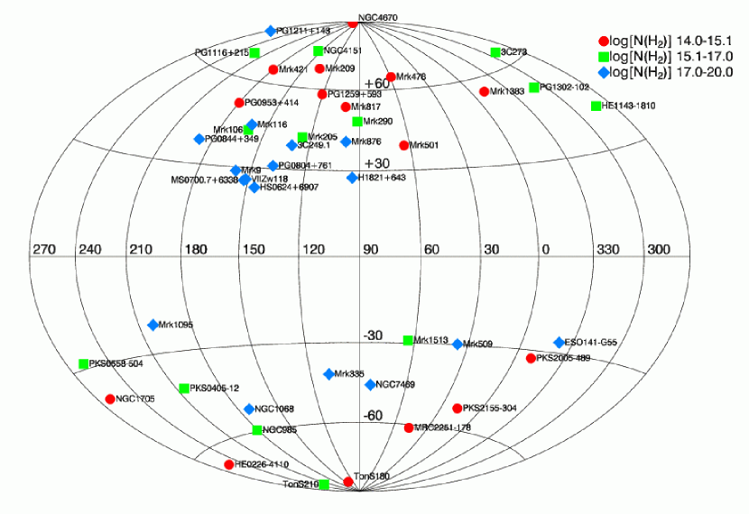
Figure 1: Aitoff projection showing locations of 45 AGN targets from our high-latitude H₂ survey. In the northern Galactic hemisphere, we identified 8 high-latitude ($b>54^{\circ}$) sight lines with low N_H2 $\leq 10^{15.1}$ cm^-2, color-coded in red. These targets suggest a widespread H₂ hole ($60^{\circ}<\ell<180^{\circ}$ and $b>54^{\circ}$). Sightlines with higher N_H2 are labeled in green and blue. We sampled targets with Galactic latitude $|b|>20^{\circ}$ to minimize absorption by interstellar gas in the Galactic disk. The low column density “H₂ Holes” at $|b|>54^{\circ}$ may be related to the “Northern Chimney” (region of low Na I absorption, Lallement et al. 2003) and the “Lockman Hole” (region near of low N_HI near $\ell=135^{\circ}-175^{\circ}$ and $b=46^{\circ}-60^{\circ}$, Lockman et al. 1986, see also Figure 10). These “H₂-clean” sight lines are ideal for FUV studies of the IGM and HVCs.

In this paper, we present a survey of H₂ toward 45 AGN at Galactic latitudes $|b|>20^{\circ}$ (see Figure 1). To produce detectable H₂, with $f_{\rm H2}>10^{-5}$, these clouds typically need hydrogen gas densities $n_{H}>$ 10 cm^-3, so that the H₂ formation rates are sufficient to offset UV photodissociation. At column densities N_H2 $>10^{15}$ cm^-2, the molecules begin to self-shield from UV photodestruction. The selection of high-latitude AGN background targets allows us to minimize the amount of H₂ from the Galactic disk, although we cannot exclude it altogether. Our high-latitude survey accompanies a larger survey (Shull et al. 2005) of H₂ toward 139 OB-type stars in the Galactic disk. These OB stars at $|b|\leq 10^{\circ}$ typically show larger H₂ column densities and greater molecular abundances than the AGN sight lines. Consequently, the AGN sight lines provide a better sample of diffuse H₂-bearing clouds above the disk, and perhaps into the low halo. Various properties of the gas, including molecular fraction, rotational temperature, and connections with infrared cirrus clouds (Gillmon & Shull 2005), suggest that the high-latitude sight lines sample a different population of diffuse absorbers than the disk survey. The halo H₂ survey may also be representative of sight lines that pass outside the inner disks of external galaxies.

The organization of this paper begins with a description of the AGN sample and our data acquisition, reduction, and analysis (§ 2). This is followed in § 3 by discussion of the results on H₂ abundances, molecular fractions, and rotational excitation. We examine both the rotational temperature, $T_{01}$, for $J=0$ and $J=1$, and the excitation temperature, $T_{\rm exc}$, for higher rotational levels. We also show the distribution of H₂ in column density and the spatial distribution throughout the northern Galactic hemisphere, particularly the conspicuous “H₂ holes” with N_H2 $\leq 10^{15}$ cm^-2 at $b>54^{\circ}$. We conclude in § 4 with a comparison of these high-latitude results to those from Galactic disk surveys by Copernicus (Savage et al. 1977) and FUSE (Shull et al. 2005).

2 DATA ACQUISITION AND REDUCTION

2.1 FUSE Observations

Table 1 lists our target names and their Galactic coordinates, source type, B magnitude, color excess E(B-V), and observational parameters. We chose our targets based on their signal-to-noise ratio (S/N), source type, and Galactic latitude. All 45 of our targets are at $|b|>20^{\circ}$, a subset of the 219 targets selected in Wakker et al. (2003) as candidates for the analysis of Galactic O VI. Of the 219 targets, Wakker et al. found 102 appropriate for O VI analysis, for which they binned the data by 5–15 pixels (the FUSE resolution element is 8–10 pixels or about 20 km s^-1) in order to meet an imposed requirement of $\rm{(S/N)_{bin}>4}$. We set a similar S/N requirement for our H₂ analysis. However, we exclude those targets that required binning by more than 8 pixels, because the loss of resolution caused by overbinning becomes problematic for the analysis of relatively narrow H₂ lines, in comparison with the typically broad ($\geq 50$ km s^-1) O VI profiles. Of the 219 targets, 55 met our requirement of $\rm{(S/N)_{bin}>4}$ or $\rm{(S/N)_{pix}>2}$ with 4-pixel binning. We excluded halo stars and restrict our sample targets to AGN plus a few starburst galaxies in order to minimize the difficulties presented by stellar continua. We checked all targets that were excluded for low S/N to see whether additional FUSE data had been acquired since the Wakker et al. (2003) survey. The additional data increased the S/N for seven of these targets sufficiently to include them in our sample.

All observations were obtained in time-tag (TTAG) mode, using the $30^{\prime\prime}\times 30^{\prime\prime}$ LWRS aperture. The resolution of FUSE varies from $R=\lambda/\Delta\lambda=15,000-20,000$ across the far-UV band, and it can also vary between observations. However, our results rely on measured equivalent widths that are effectively independent of instrumental resolution. Data were retrieved from the archive and reduced locally using CalFUSE v2.4. The CalFUSE processing is described in the FUSE Observers Guide (http://fuse.pha.jhu.edu). Raw exposures within a single FUSE observation were coadded by channel mid-way through the pipeline. This can produce a significant improvement in data quality for faint sources (such as AGN) since the combined pixel file has higher S/N than the individual exposures, and consequently the extraction apertures are more likely to be placed correctly. Combining exposures also speeds up the data reduction time substantially.

Because FUSE has no internal wavelength calibration source, all data are calibrated using a wavelength solution derived from in-orbit observations of sources with well-studied interstellar components (Sahnow et al. 2000). This process leads to relative wavelength errors of up to 20 km s^-1 across the band, in addition to a wavelength zero point that varies between observations. For targets with data from multiple observations, the spectra from separate observations were coaligned and coadded to generate a final spectrum for data channels LiF1a and LiF2a (the other six data channels were not used in our analysis). The coalignment was performed on one single line per channel: Ar I at 1048.22 Å for LiF1a, and Lyman (1-0) P(3) at 1099.79 Å for LiF2a. Since we did not correct for possible relative wavelength errors across the wavelength range before coadding, our method of using a single line to perform the alignment may blur out weak lines at wavelengths well away from 1048.22 Å (LiF1a) and 1099.79 Å (LiF2a).

Once the final coadded spectra have been obtained, there may still be errors in the wavelength solution. Because the 21 cm spectra are acquired with ground-based telescopes, their wavelength solution is more accurate than that of FUSE data. We attempted to correct the FUSE wavelength solution by plotting the 21 cm emission line and Ar I 1048.22 Å absorption line in velocity space and shifting the FUSE spectra to align the centroids. Although it is not necessarily the case that the neutral gas (H I) must align in velocity with low-ionization metals (Ar I, Si II, Fe II) or with H₂, it is a plausible assumption that provides a standard technique for assigning the FUSE wavelength scale. Although relative wavelength errors may exist across the full wavelength range, we place our trust in the wavelength solution near 1048 Å and use H₂ lines in the (4-0) and (5-0) Lyman bands between 1036–1062 Å to determine the velocity of the H₂ clouds (see § 2.2). The S/N of the co-added data ranges from 2–11 per pixel, and it also varies with spectral resolution, which is not fixed in our survey. Most of the data were binned by 4 pixels before analysis, with the rare case of binning by 2 or 8 pixels.

2.2 Data Analysis

In our analysis of H₂, we use the signature absorption bands in the FUSE LiF channels between 1000 and 1126 Å. These bands arise from the Lyman and Werner electronic transitions from the ground ($v=0$) vibrational state and rotational states $J=0-7$. Wavelengths, oscillator strengths ($f$), and damping constants for these lines were taken from Abgrall et al. (1993a,b). Because of the rapid decrease in FUSE sensitivity and decreased S/N in the SiC channels at wavelengths less than 1000 Å, we restrict our analysis to ten vibrational-rotational bands, Lyman (0-0) to (8-0) and Werner (0-0). Additional information can be gleaned from higher vibrational bands ($\lambda<1000$ Å) in the SiC channels, but we do not present this data here. To maximize efficiency, we restricted our analysis to the LiF1a and LiF2a channels, which provide the best combination of wavelength coverage and sensitivity. These channels provide higher S/N than the SiC channels in this wavelength range and include the Lyman (2-0) and (1-0) bands.

Seven AGN sight lines show H₂ absorption in $J=4$, and absorption lines from $J=5$ were detected toward one target (HS 0624+6907). Approximately one-third (15) of the sight lines show substantial H₂ column densities, ranging from log N_H2 = 18.0 – 19.8, with damping wings in the $J=0$ and $J=1$ lines. Half the AGN spectra show weaker H₂ absorption with log N_H2 $\approx$ 14 – 17. A summary of our results appears in Table 2, where we list H₂ column densities in each rotational state ($J=0-5$) and the doppler parameter ($b$) from the CoG.

Our analysis routines are adapted from Tumlinson et al. (2002), who developed our standard software for analyzing H₂. These routines allow us to determine equivalent widths for as many H₂ lines as possible, and then to apply a curve of growth (CoG) to arrive at column densities in individual rotational states, $N(J)$. From this information, we can infer various properties of the gas. We fitted all detected H₂ lines between 1000 and 1126 Å that are not visibly compromised by continuum problems or line blending, using either a Gaussian or Voigt profile in order to measure the equivalent width, $W_{\lambda}$. For most sight lines, the fits to the absorption lines are carefully tailored on a line-by-line basis to choose the correct continuum and adjust for any line blending. When a proper fit to a line or group of lines has been obtained, the equivalent width $W_{\lambda}$, uncertainty in $W_{\lambda}$, and central wavelength are stored in an electronic table for use by the CoG fitting routines. In select cases, we fitted the $J\geq 2$ lines with a more automated routine, also described in Tumlinson et al. (2002), which queries the user at each wavelength corresponding to an H₂ line and allows it to be fitted with a single Gaussian component. This routine is useful for targets with relatively flat continua and minimal line blending. The automated routine also stores $W_{\lambda}$, uncertainty in $W_{\lambda}$, and central wavelength in a table. The $J=0$ and 1 lines are fitted by hand with a Voigt profile since they may be strong enough to have non-Gaussian profiles. For lines between 1036–1062 Å in the Lyman (5-0) and (4-0) bands, with well-determined centroids, we converted the central wavelength to a velocity using the Doppler formula and then averaged the velocities. We list these H₂ cloud velocities (LSR) in Table 3, together with velocities of the various 21-cm emission components (Wakker et al. 2003).

A single sight line is likely to intercept many clouds containing H₂, that may or may not be offset in velocity. One of the potential sources of systematic uncertainty is our inability to resolve components of H₂ absorption by different clouds along the line of sight. At the FUSE resolution of 20 km s^-1, we typically cannot separate absorption components in the “LSR core”, from $-20$ to $+20$ km s^-1. Components separated by $\geq$ 30 km s^-1 can sometimes be resolved, depending on the line strengths and widths. We have 24 targets in common with Richter et al. (2003), who focused on H₂ in intermediate velocity clouds with $|v|=30-90$ km s^-1. They report the existence of an IVC in 7 of our sight lines and cite a possible IVC in 6 others. Because we focus on low-velocity H₂, we generally avoid IVCs in our line fitting. We have determined the column density for an IVC in three cases: 3C 273, Mrk 876, and NGC 4151. For 3C 273, we measured H₂ at +25 km s^-1, which we do not consider a true IVC. For Mrk 876, we fitted the IVC lines along with the LSR core lines (double component fits). For NGC 4151, the H₂ lines arise mainly from IVC gas, but they may have contributions from an LSR component. Out of the 7 targets with confirmed IVCs, it is possible in one case that the IVC contributed to our measured LSR H₂ lines. For the 6 targets with possible IVCs, it is possible in four cases that an IVC contributed to our fitted LSR H₂ lines. We also note 4 targets where Richter et al. (2003) claim “no evidence” for an IVC, but we believe an IVC contributed to our measured H₂ lines. Our comments on velocity components and IVCs are summarized in Table 3. Multiple unresolved components in the LSR core, as well as possible contributions from IVCs, may produce a composite CoG [$b$ and $N(J)]$ that reflects the properties of the different velocity components.

Once the line fitting is complete, the software described in Tumlinson et al. (2002) produces an automated least-squares fit to a CoG with a single doppler $b$ parameter for all $J$ levels. For the two sight lines noted above (3C 273 and Mrk 876), we make a two-component fit for the LSR core and IVC. Table 2 gives the best-fit values of $N(J)$ and single-$b$, with 1 $\sigma$ confidence intervals. For low-S/N sight lines or those with low column densities, it is sometimes difficult to measure enough lines to constrain the CoG. This results in large error bars on $N(J)$ and $b$. In some cases, model spectra of varying $N(J)$ and $b$ are overlaid on the spectrum to narrow the range of reasonable values. In many cases, the Lyman (1-0) and (0-0) $J=3$ lines are crucial in constraining the $b$ value. Large error bars on $N(J)$ and $b$ often result when these lines are absent.

For sight lines with no discernable H₂ lines, our methodology is as follows. We place upper limits on the equivalent widths of the strong Lyman (7-0) R(0) and R(1) lines and convert these limits to column density limits assuming a linear CoG. For the (4 $\sigma$) limiting equivalent width of an unresolved line at wavelength $\lambda_{0}$, we use the following expression:

$$W_{\lambda}^{\rm lim}=\frac{4\lambda_{0}}{(\lambda/\Delta\lambda)(\rm{S/N})}\;.$$ (1)

Since the resolution of FUSE varies across the band, we conservatively assume $R=\lambda/\Delta\lambda\approx 15,000$ for all upper limits. The limiting equivalent widths range from 8 mÅ for high-S/N data to 43 mÅ for low-S/N data. This corresponds to a limiting column density range of log N_H2 $>13.8-14.6$. The upper limits are included in Table 2.

2.3 H I COLUMN DENSITIES

In order to fully interpret our observations of interstellar H₂, we obtain supplementary data on the atomic hydrogen (H I) column densities associated with the observed H₂. Since our sample of 45 sight lines is a subset of that in Wakker et al. (2003), we use their compilation of the 21-cm spectrum, as well as the component structure and N(H I) determined by fits to the data. They collected 21-cm spectra from the following sources: Leiden-Dwingeloo Survey ($35^{\prime}$ beam), Villa Elisa telescope ($34^{\prime}$ beam), Green Bank 140-ft telescope ($1^{\prime}$ beam), and the Effelsberg telescope ($9.^{\prime}7$ beam). Wakker et al. (2003) provide the 21-cm spectrum, as well as the component structure and N(H I) determined by fits to the data.

To derive N_HI, we must determine which of the H I components are physically associated with the observed H₂. This assignment can be uncertain and somewhat subjective, so we take care to choose a “best value” and a range of H I column densities, from N_min to N_max. Figure 2 illustrates our technique for Mrk 509, with the 21-cm emission line, H₂ Lyman (4-0) R(0) absorption line, and Ar I 1048.22 Å absorption line aligned in velocity space. We shift the FUSE data with respect to the 21-cm data in order to align the H I emission and Ar I absorption as described in § 2.1. We then select as N_best the sum of column densities in the H I components that are associated with H₂ absorption, based on the coincidence of the radial velocities. Of these selected components, at the 20 km s^-1 resolution of FUSE, there remains some uncertainty about which are actually associated with H₂. In order to reflect this systematic uncertainty and to be conservative with errors, we adopt a range for the H I column density, including a floor of systematic uncertainty of $\pm 0.03$ in log N_HI. For the lower limit, N_min, we use the smallest individual column density that could be responsible for the H₂ absorption within the velocity range of the R(0) or R(1) line widths. For the upper limit, N_max, we use the sum of all the H I column densities that can associated kinematically with the H₂. For sight lines with no discernable H₂ lines, we adopt a lower limit on N_HI as the smallest of the components that is not classified as an IVC or HVC and that satisfies the condition N_HI $\geq 10^{19}$ cm^-2.

Further systematic uncertainty arises from the larger beam size of the 21-cm data compared with the pencil-beam sight lines of the H₂ data. It has been shown that a smaller beam gives a better approximation to the H I column density in the pencil beam (Wakker & Schwarz 1991; Wakker et al. 2001, 2002). On the other hand, Lockman & Condon (2005), using the $9^{\prime}.8$ Green Bank telescope, find that N_HI is highly correlated spatially. In Table 4, we provide various information on H₂ and H I, as well as the 21-cm beam size.

3 RESULTS

3.1 General Results

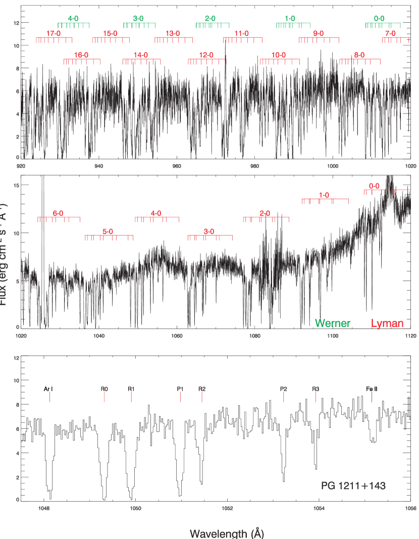
Figure 3: Upper two panels: FUSE spectrum of PG 1211+143, showing expected locations of (0-0) through (17-0) H₂ Lyman bands (red) and (0-0) through (4-0) Werner bands (green). This sight line has log N_H2 = $18.38^{+0.15}_{-0.14}$ in $J=0-3$. Lower panel: Blowup of the (4-0) Lyman band of H₂, showing R(0), R(1), P(1), R(2), P(2), and R(3) absorption lines from $J$ = 0, 1, 2, and 3 together with interstellar lines of Ar I $\lambda 1048.220$ and Fe II $\lambda 1055.262$.

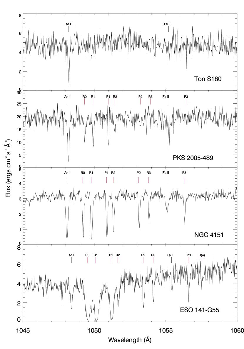
Figure 4: Examples of FUSE spectra of four AGN, showing increasing H₂ column densities from the Lyman (4–0) band. First panel: Ton S180 shows no detectable to a limit log N_H2 $<14.37$ ($<13.98$ in $J=0$ and $<14.14$ in $J=1$). Second panel: PKS 2005-489 with log N_H2 = $15.07^{+0.10}_{-0.10}$. Third panel: NGC 4151 with log N_H2 = $16.70^{+0.93}_{-0.31}$. Fourth panel: ESO 141-G55 with log N_H2 = $19.32^{+0.07}_{-0.07}$.

As noted earlier, H₂ absorption is present in most of the high-latitude sight lines. Figure 3 shows a sample FUSE spectrum of PG 1211+143, an AGN sight line that has been studied extensively with both FUSE and Hubble Space Telescope (HST) by Penton, Stocke, & Shull (2004) and Tumlinson et al. (2005). This sight line has a substantial column density, log N_H2$=18.38^{+0.15}_{-0.14}$, producing a clear H₂ band structure throughout the FUV. The lines are saturated, but strong damping wings are not yet present. Figure 4 shows a sequence of four FUSE spectra of AGN, in order of increasing H₂ column density. These range from Ton S180, where we detect no H₂ to a ($4\sigma$) limit log N_H2 $<14.37$ ($<13.98$ in $J=0$ and $<14.14$ in $J=1$), to ESO 141-G55, in which log N_H2 = $19.32\pm 0.07$ with prominent damping wings in the R(0) and R(1) lines arising from $J=0$ and $J=1$. This montage shows a number of H₂ absorption lines from $J=0-4$ in the important Lyman (4-0) band, along with interstellar lines of Ar I and Fe II, the former of which is used to define the LSR velocity scale.

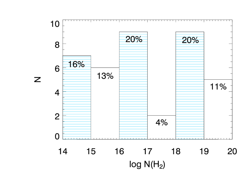
Figure 5: Distribution of N_H2 (the LSR absorption only) for 38 of our 45 AGN sight lines. An additional 7 sight lines (16% of the sample) showed no detectable low-velocity H₂ above a threshold, log N_H2 = 13.8–14.6, depending on the S/N (2-11 per pixel) and resolution ($R=15,000-20,000$ for FUSE). The dip in numbers between log N_H2 = 17 – 18 may divide two populations (see also Fig. 9), although this column density bin is sensitive to CoG uncertainties and is based on small numbers of sight lines.

Table 2 lists the H₂ column densities in individual rotational states, $J=0-5$ and the doppler ($b$) parameters from the CoGs. Figure 5 displays the distribution of H₂ column densities, from the detectable limit, log N_H2 $\approx 14.2$, up to the maximum observed value log N_H2 $\approx 19.8$. Except for the dip at log N_H2 = 17–18, the distribution is fairly flat in column density. Small-number statistics preclude any firm conclusion about whether this dip is real, but it does suggest two populations of H₂ absorbers. For each sight line, Table 4 lists the total H₂ and H I column densities, molecular fraction ($f_{\rm H2}$), rotational temperature, $T_{01}$, of $J=0$ and $J=1$ states, and the excitation temperature, $T_{\rm exc}$, that characterizes the higher-$J$ states. These temperatures were derived by least-squares fits of the column densities, $N(J)$, to the form,

$$\frac{N(J)}{Z_{\rm H2}}=g_{J}\exp\left(-\frac{E_{J}}{kT}\right)\;.$$ (2)

Here, $g_{J}=g_{S}(2J+1)$ is the statistical weight of rotational level $J$, with spin factor $g_{S}=1$ or 3 for para- or ortho-H₂, respectively, $E_{J}$ is the excitation energy of level $J$, $Z_{\rm H2}$ is the H₂ rotational partition function, and $T$ denotes $T_{01}$ for rotational states $J$ = 0 and 1 or $T_{\rm exc}$ for excited states $J\geq 2$.

3.2 Molecular Fraction

Among the parameters listed in Table 4 is the average molecular fraction,

$$f_{\rm H2}=\frac{\rm{2N(H_{2})}}{\rm{N(H~{}I)+2N(H_{2})}}\;,$$ (3)

which expresses the fraction of all hydrogen atoms bound into H₂ molecules. We define the total column density of hydrogen as N${}_{\rm H}\equiv$ N_HI + 2N_H2, derived from N_H2, the H₂ column density in all rotational states, and N_HI, the neutral hydrogen column density derived from 21-cm emission (§ 2.3). Error bars on log N_H2 are found by propagating the uncertainties on log N(0) and log N(1), which dominate the H₂ column density.

In optically thin clouds, the density of molecules can be approximated by the equilibrium between formation and destruction,

$$f_{\rm H2}\approx\frac{2n_{H}R(T_{\rm gas},T_{\rm gr},Z)}{\beta\;\langle f_{\rm diss}\rangle}\approx(10^{-5})R_{-17}\;n_{30}\left(\frac{\beta_{0}}{\beta}\right)\;.$$ (4)

In this formula, the numerical value for $f_{\rm H2}$ is scaled to fiducial values of hydrogen density, $n_{H}$ (30 cm^-3), H₂ formation rate coefficient, $R$ ($10^{-17}$ cm³ s^-1), and mean H₂ pumping rate in the FUV Lyman and Werner bands, $\beta_{0}=5\times 10^{-10}$ s^-1. The H₂ photodissociation rate is written as $\langle f_{\rm diss}\rangle\beta$, where the coefficient $\langle f_{\rm diss}\rangle\approx 0.11$ is the average fraction of FUV excitations of H₂ that result in decays to the dissociating continuum. The H₂ formation rate per unit volume is written as $n_{H}n_{\rm HI}R$, where $R$ depends on the gas temperature, grain surface temperature, and gas metallicity ($Z$). The metallicity dependence comes from the assumed scaling of grain-surface catalysis sites with the grain/gas ratio. For sight lines in the local Galactic disk, this rate coefficient has been estimated (Jura 1974) to range from $R=(1-3)\times 10^{-17}$ cm³ s^-1 for solar metallicity. This standard value for $R$ is expected to apply when H I can stick to grain surfaces at suitably low temperatures of gas ($T_{\rm gas}\leq 300$ K) and grains ($T_{\rm gr}\leq 100$ K) as discussed by Shull & Beckwith (1982) and Hollenbach & McKee (1979). Although some infalling halo gas may have metallicities as low as 10–25% solar, as in HVC Complex C (Collins et al. 2003), we expect that most of the H₂-bearing clouds in the low halo will have near-solar abundances and grain/gas ratios.

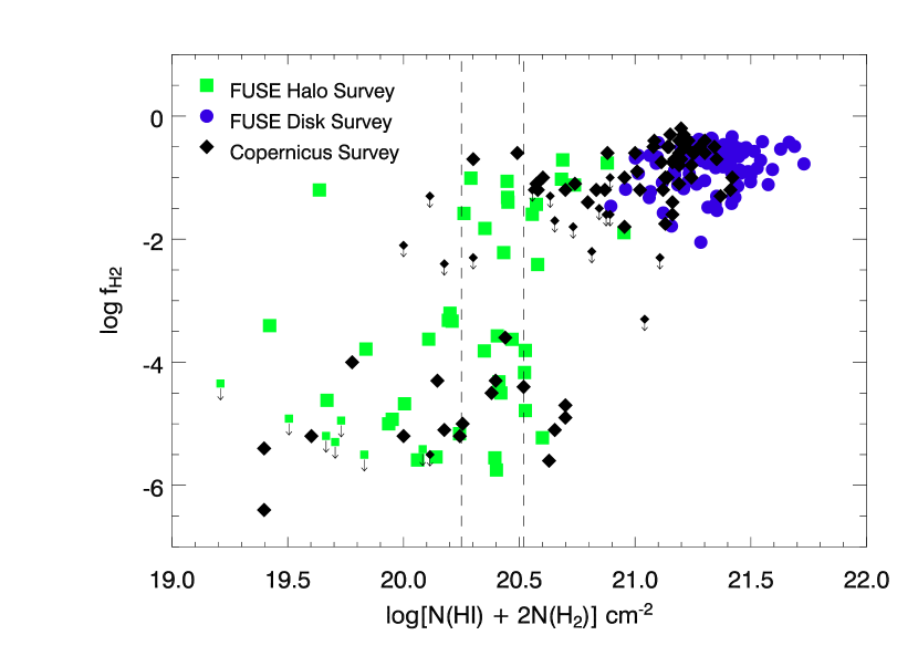
Figure 6: Transitions in molecular fraction, $f_{\rm H2}$, with total hydrogen column density, N_H = (N_HI + 2N_H2). In our FUSE survey of 45 high-latitude sight lines, the transition occurs at log N${}_{\rm H}\approx 20.38\pm 0.13$, approximately a factor of two below the transition (log N_H = 20.7) in the Copernicus survey (Savage et al. 1977). This shift to lower N_H could arise from reduced photodissociation (lower UV field), from enhanced H₂ formation rates (higher $n_{H}$ in compressed cirrus clouds) or both.

Once sufficient column density of H₂ builds up, with N_H2 $\geq 10^{15}$ cm^-2, the cloud becomes optically thick in individual Lyman and Werner lines, and the dissociation rate begins to drop, owing to self-shielding in the lines. The molecular fraction rises and makes an abrupt transition to much higher values, $f_{\rm H2}\geq 10^{-2}$, when the strong R(0) and R(1) lines develop damping wings at N_H2 $\geq 10^{18}$ cm^-2. For our halo survey, Figure 6 shows the molecular fractions, $f_{\rm H2}$, vs. total H column density. The molecular fraction rises from low values, $f_{\rm H2}\approx 10^{-5.5\pm 0.5}$, to values above $10^{-2}$, typical of sight lines in the disk. The transition for halo sight lines occurs over a range log N${}_{\rm H}\approx 20.2-20.5$ (we quote a transition at log N${}_{\rm H}=20.38\pm 0.13$), approximately a factor of two below the similar transition in the Milky Way disk at log N${}_{\rm H}=20.7$ (Savage et al. 1977; Shull et al. 2005). The precise location of the halo transition is not well determined from just 45 sight lines. Some broadening of the distribution is expected, since these sight lines may sample a mixture of gas in the low halo (low $f_{\rm H2}$) and denser clouds in the disk (higher $f_{\rm H2}$).

The large observed fluctuations in H₂ column density require a very patchy ISM in the halo. For 25 sight lines in the northern Galactic hemisphere at latitude $|b|\geq 20^{\circ}$, the mean total H₂ column density is $\langle{\rm N}_{\rm H2}\sin(b)\rangle=16.80$, with a range from $10^{14}$ to $10^{19.8}$ cm^-2. In the Copernicus H₂ survey, Savage et al. (1977) found an average mid-plane density $n_{0}$(H₂) = 0.036 cm^-3 for 76 stars, which they increased to 0.143 cm^-3 after correction for sampling biases due to reddening. If the H₂ absorption was distributed smoothly in an exponential layer, $n(z)=n_{0}\exp(-z/h)$, with scale height $h$, the integrated column density toward a quasar at latitude $b$ would be N_H2 $=n_{0}h/\sin(b)$. For $h\approx 100$ pc, the column density would exceed N_H2 = $10^{19}$ cm^-2, even at high latitude. Obviously, a smooth distribution of H₂ is in disagreement with our observations.

The obvious explanation for the wide variations in N_H2 is a clumpy medium. However, the observed range (and fluctuations) in N_H2 constrain the geometry and hydrogen density of the H₂-bearing “clouds”. For example, consider an ensemble of spherical clouds of radius $r_{\rm cl}=(3~{}{\rm pc})r_{3}$ and density $n_{H}=(30~{}{\rm cm}^{-3})n_{30}$. If H₂ is in formation-destruction equilibrium with the mean FUV radiation field, the molecular density inside the cloud is:

$$n_{\rm H2}\approx\frac{n_{H}^{2}\;R}{0.11\beta}\approx(1.64\times 10^{-4}~{}{\rm cm}^{-3})n_{30}^{2}R_{-17}\left(\frac{\beta_{0}}{\beta}\right)\;,$$ (5)

where, as before, we have scaled the H₂ formation rate coefficient $R$ to $10^{-17}$ cm³ s^-1. The typical H₂ column density through one such cloud would be

$$N({\rm H}_{2})=\frac{4n_{\rm H2}r_{\rm cl}}{3}\approx(2\times 10^{15}~{}{\rm cm}^{-2})n_{30}^{2}R_{-17}\left(\frac{\beta_{0}}{\beta}\right)~{}r_{3}\;.$$ (6)

In order to explain the total H₂ column density, a sight line to an AGN would have to intercept hundreds of such absorbers. The fluctuations in the number of clouds along different sight lines would then be quite small, certainly much less than the range observed. On the other hand, a smaller number of dense, sheetlike clouds, with a patchy distribution like the infrared cirrus, would be consistent with the data. These clouds would each have more N_H2, so the required number of interceptions would be smaller. Some high-latitude sight lines would have very large column densities, while others would be quite low, as in the “H₂ Holes” that we discuss in § 3.5. We return to the cirrus model in § 3.4.

3.3 Rotational Temperature

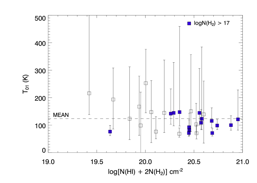
Figure 7: Mean rotational temperature in our Galactic high-latitude survey is $\langle T_{01}\rangle=124\pm 8$ K (median 121 K). For 15 sight lines with log N_H2 $\geq 17$ (solid squares), we find $\langle T_{01}\rangle=109\pm 7$ K. These temperatures are somewhat higher than those found in the Copernicus H₂ survey ($77\pm 17$ K, Savage et al. 1977) and in our FUSE Galactic disk survey ($86\pm 20$ K, Shull et al. 2005). The range of $T_{01}$ is 68–252 K, consistently higher than the Galactic disk values, all but two of which lie between 55–120 K.

Figure 7 shows the $J$ = 0–1 rotational excitation temperature, $T_{01}$, which can measure the kinetic temperature in dense clouds, where H⁰–H₂ and H⁺–H₂ collisions dominate the mixing of the $J=0$ and $J=1$ rotational levels. The solid squares indicate high-N_H2 sight lines, where models suggest that the rotational temperature should be close to the gas kinetic temperature. The quantity $T_{01}$ is obtained from the expression

$$T_{01}=\frac{\Delta E_{01}/k}{\ln[(g_{1}/g_{0})N(0)/N(1)]}\;,$$ (7)

where $g_{1}/g_{0}=9$ is the ratio of the statistical weights of the $J=1$ and $J=0$ rotational levels, and $\Delta E_{01}/k=170.5$ K is the excitation temperature of the $J=1$ level.

To assess the statistical properties of the H₂ rotational temperature in the halo, we selected 29 sight lines with sufficiently small error bars on N(0) and N(1) to provide useful information on $T_{01}$. The halo rotational temperatures range from $T_{01}$ = 68–252 K, with a median of 139 K, a range that extends higher than the FUSE Galactic disk values, all but two of which lie between 55–120 K (Shull et al. 2005). For these 29 sight lines, the mean rotational temperature, $\langle T_{01}\rangle=124\pm 8$ K, is larger than the values found in the Copernicus H₂ survey ($77\pm 17$ K, Savage et al. 1977) and in our FUSE Galactic disk survey ($86\pm 20$ K, Shull et al. 2005). For the 15 sight lines with log N_H2 $\geq 17$, we find $\langle T_{01}\rangle=109\pm 7$ K.

An elevated kinetic temperature in the low halo could signal a shift in thermal balance between UV photoelectric heating by dust grains and radiative cooling, primarily by the [C II] 158 $\mu$m fine structure line. Both the heating and cooling rates should depend on the gas-phase metallicity, if the grain abundance scales with metallicity. In the low halo, we expect $0.1<(Z/Z_{\odot})<1.0$, with most clouds showing 30%–100% solar metallicities. Even though the abundances for these clouds might differ, the equilibrium gas temperature should be nearly independent of metallicity (Shull & Woods 1985), owing to cancelling dependences of heating and cooling on $Z$. The distribution of measured $T_{01}$ is broad, and some of the sight lines have large error bars. The median temperature is 121 K, although a minimum-$\chi^{2}$ fit gives $83\pm 6$ K. Therefore, it may be premature to quote a higher temperature of these clouds. Additional studies of high-latitude sight lines would be most helpful.

3.4 Excitation Temperature

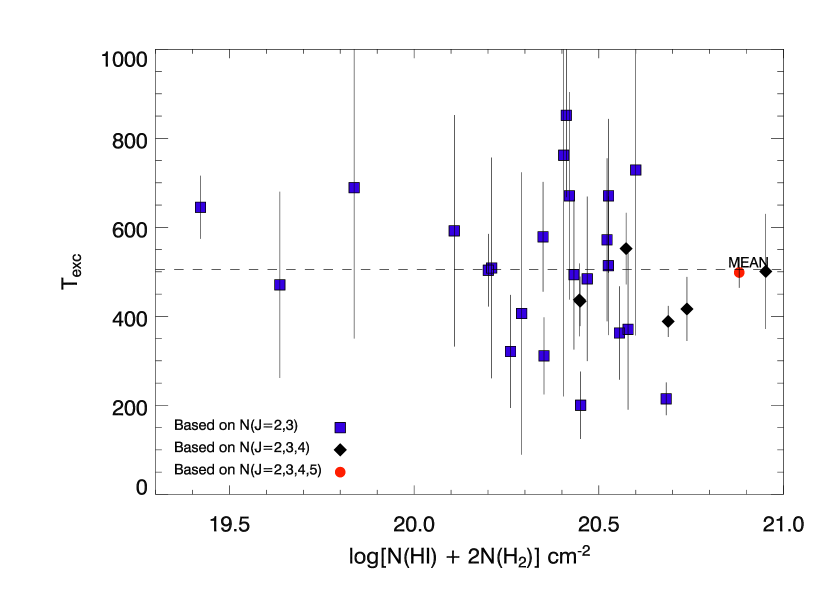
Figure 8: The mean excitation temperature for $J\geq 2$ is $\langle T_{\rm exc}\rangle=505\pm{28}$ K (median 501 K), based on 30 sight lines with detectable $J=3$ lines (in some cases $J=4$ and $J=5$). This value is slightly larger than the mean, $326\pm 125$ K, seen in the FUSE disk H₂ survey (Shull et al. 2005). The distribution of $T_{\rm exc}$ is a measure of non-thermal excitation by UV pumping and perhaps H₂ formation on grain surfaces (Browning et al. 2003).

Figure 8 shows the higher-$J$ excitation temperature, $T_{\rm exc}$, which reflects non-thermal UV fluorescent pumping of the high-$J$ levels. The mean excitation temperature in the Galactic halo survey is $\langle T_{\rm exc}\rangle=505\pm 28$ K, with a range from 200–852 K. The median value is 501 K, while a $\chi^{2}$ fit to a constant temperature gives $416\pm 15$ K. These values are similar to those seen by the Copernicus survey (Spitzer & Jenkins 1975; Shull & Beckwith 1982), but slightly higher than that ($326\pm 125$ K) found in our FUSE disk survey (Shull et al. 2005).

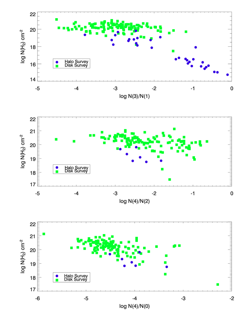
Figure 9: Ratios of rotational-state column densities for $J=3/1$, $J=4/2$, $J=4/0$ vs. N_H2 for sight lines in our surveys in the Galactic halo (blue) and Galactic disk (green). Of the 45 halo sight lines, 8 have measured column densities for both $J=3$ and $J=4$, while 32 have $J=3$ but lack detectable $J=4$ because of insufficient total N_H2. For all sight lines with log N_H2 $\geq 18$, the degree of rotational excitation is comparable (Shull et al. 2005), except for a population of 16 halo sight lines with low N_H2 and highly excited $J=3$ [log N(3)/N(1) $\geq-1.5$]. A comparison of the high-N_H2 data with models of H₂ formation and rotational excitation (Browning et al. 2003) suggests that the UV radiation fields in the low Galactic halo and disk are similar. To produce the observed shift to lower N_H in the transition of $f_{\rm H2}$, the H₂ formation rate may be enhanced in the halo absorbers, because of higher $n_{H}$ in compressed cirrus clouds.

Figure 9 shows three ratios of high-$J$ rotational states: N(3)/N(1), N(4)/N(2), and N(4)/N(0) versus log N_H2 in both low-latitude and high-latitude H₂ surveys. The high-latitude survey contains 32 sight lines with $J=3$ measurements. Of these, only 8 sight lines have measured values of both N(3) and N(4), and all have substantial column densities, log N_H2 $\geq 18$. The $J$-ratios in these absorbers reflect the relative effects of UV excitation and collisional de-excitation for para-H₂ ($J=0$ and 2) and ortho-H₂ ($J=1$ and 3), respectively. For the N(4)/N(2) ratio, the approximate ranges for the surveys are:

• High-Latitude: log N(4)/N(2) = $-2.8$ to $-1.8$ and log N_H2 = 18.5–20.0

• Low-Latitude: log N(4)/N(2) = $-4.0$ to $-1.0$ and log N_H2 = 19.5–21.0

In general, these two distributions appear to cover similar ranges, particularly for absorbers with log N_H2 $\geq 18$. The greatest distinction between these populations occurs for the ratio N(3)/N(1) in a subset of 16 high-latitude sight lines with low H₂ column density, log N_H2 = 14–17, and have ratios log N(3)/N(1) = $-1.5$ to $-0.5$, well above the mean value in the disk ($-3.0$). These clouds are more optically thin in the dissociating FUV radiation, and thus have not built up large column densities in $J=0$ or 1. For the 8 sight lines with data for both $J=3$ and $J=4$, the degree of UV excitation appears similar in both latitude regimes. This result is consistent with models of the Galactic radiation field above the disk (Wolfire et al. 1995; Bland-Hawthorn & Maloney 1999), which suggest that the FUV radiation field drops by only $\sim 50$% at elevation $z\approx 1$ kpc.

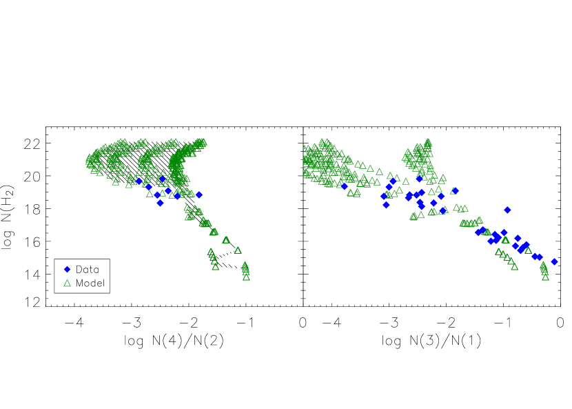
Figure 10: Models of H₂ rotational excitation ratios, $N(J)$, using the code of Browning, Tumlinson, & Shull (2003). Plots show ratios, $N(4)/N(2)$ and $N(3)/N(1)$, versus N_H2, for data (blue points, same as in Fig. 9) and for a grid of models (green points). Models assume the mean Galactic H₂ formation rate ($R=3\times 10^{-17}$ cm³ s^-1), and a range of parameters, FUV radiation fields, varying by a factor of two above and below the mean ISM value ($I_{\rm FUV}=2\times 10^{-8}$ photons cm^-2 s^-1 Hz^-1 between 912–1120 Å). The model grid ponts include variations in cloud temperatures ($T=$ 20–150 K) and density ($n_{H}$ = 5–800 cm^-3). Note the good agreement between data and models, which show increasing excitation, $N(3)/N(1)$, for “thinner” clouds, log N_H2 $\leq 18$.

The high-latitude sight lines typically have a factor of 30 lower H₂ column densities than those in the disk. For the disk absorbers, the highly excited $J$ populations probably reside in surface layers surrounding a core with greater column densities in N(0) and N(1). Our recent models of H₂ formation and excitation processes (Browning et al. 2003) can be used to estimate the effects UV radiation field and gas density from ratios such as N(4)/N(2) or N(3)/N(1). Figure 10 shows models that confirm these predictions in our high-latitude data.

Taken together, these ratio distributions suggest that the degree of rotational excitation in the high-latitude sight lines is comparable to that in our disk survey (Shull et al. 2005) for high-N_H2 sight lines. At first glance, this conclusion may seem inconsistent with the observed distribution of molecular fractions, $f_{\rm H2}$, with column density, N_H. For the halo sight lines, the transition in $f_{\rm H2}$ occurs at 50% lower N_H. As shown in equation (4), the molecular fraction scales as $f_{\rm H2}\propto(n_{H}R/\beta)$. Thus, a shift in the distribution could arise either from a reduced rate of H₂ dissociation (low $\beta$) or an increased rate of H₂ formation, $n_{H}R$, on grain surfaces. The formation rate could be increased by a higher grain abundance or surface area (unlikely at the metallicities of halo clouds) or by a higher density $n_{H}$ resulting from cloud compression. Because we cannot supply clear evidence for an anomalously efficient population of dust grains in these high-latitude clouds, we favor the high-$n_{H}$ explanation. However, additional studies of the dust properties of these absorbers would be useful.

Therefore, our best explanation of the observed $J$-ratios and the shift in the $f_{\rm H2}(N_{H})$ transition is that comparable UV dissociation rates in the halo and disk are offset by enhanced grain formation of H₂ arising from halo clouds with higher density than in the disk. For example, these halo H₂ absorbers may be compressed sheets associated with the IR cirrus, as suggested for the strong H₂ toward ESO 141-G55 (Shull et al. 2000). We have followed up this idea (Gillmon & Shull 2005), where we find a clear association between H₂ and IR cirrus clouds. Specifically, we see the same self-shielding transition of $f_{\rm H2}$ versus 100 $\mu$m cirrus intensity as seen with N_H. This suggests that the cirrus clouds with N_H2$\geq 10^{18.5}$ cm^-2 have a substantial molecular content, ranging from 1–30%.

3.5 Holes in the H₂ Distribution

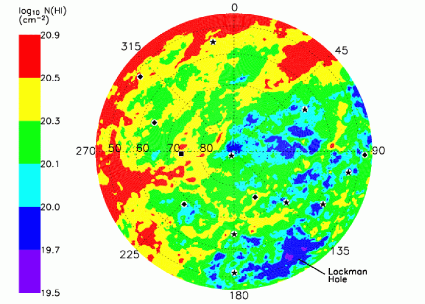
Figure 11: Locations in northern Galactic hemisphere ($b>45^{\circ}$) of 14 high-latitude AGN sight lines (white circles). The symbols inside white circles indicate log N_H2 in the ranges: 14.0–15.1 (Star); 15.1–17.0 (Diamond); 17.0–20.0 (Square). The targets sample the distribution of N_HI in the Leiden Dwingeloo Survey (Hartmann & Burton 1997), colored as deep-blue (log N_HI = 19.7–20.0) or light-blue (20.0–20.1). Gas at higher N_HI is shown in green, yellow, or red. The extended Lockman Hole (log N_HI $\approx$ 19.5–20.0) is seen in blue/purple ($\ell=135^{\circ}-175^{\circ}$ and $b=46^{\circ}-60^{\circ}$) at lower right.

Many of our high-latitude AGN targets lie behind regions of low H₂ column density. As noted earlier, most of our sight lines show Galactic H₂ absorption with detected column densities ranging from N_H2 $=10^{14.17-19.67}$ cm^-2. In the northern Galactic hemisphere, 8 sight lines have weak H₂ absorption (N_H2 $\leq 10^{15}$ cm^-2) located between $l=60^{\circ}-180^{\circ}$ at $b>54^{\circ}$. We have identified these high-latitude regions as “H₂ holes”, a patchy network of interstellar gas with both low 21-cm emission and low H₂ absorption (Figure 11).

The 8 sight lines through the H₂ holes provide special locations to probe diffuse halo gas, including large-scale halo structures, IVCs, and HVCs. The structure of these holes may have been shaped by infalling H I clouds, as well as by outflowing gas from the “Northern Chimney”, an interstellar cavity inferred from low Na I absorption at $z\leq 300$ pc (Lallement et al. 2003). Large portions of the holes have N_H2 $\leq 10^{15}$ cm^-2. These regions of low N_H2 are analogous to the “Lockman Hole” of low N_HI (Lockman et al. 1986), but they have much greater extent. Figure 11 compares our H₂ survey with the distribution of N_HI in the northern Galactic hemisphere at $b\geq 45^{\circ}$.

4 DISCUSSION AND SUMMARY

Our FUSE high-latitude survey was able to probe molecular fractions below and above the transition value at log N${}_{\rm H}\approx 20.38\pm 0.13$. We compared this transition to that seen in the Galactic disk surveys (Savage et al. 1977; Shull et al. 2005). Our sample, and possibly an enlarged future survey, can be used to examine fundamental properties of H₂, tied to O VI, H I, and IR cirrus, in an optically thin regime (log N_H2 $<17$) inaccessible to FUSE in the Galactic disk. These low-column clouds provide important tests of our theoretical models of H₂ formation, destruction, and excitation in optically-thin environments, where FUV radiation dominates the $J$-level populations.

These high-latitude sight lines are also relevant for far-UV studies of interstellar gas, intergalactic gas, and HVCs, since they provide “H₂-clean” sight lines with minimal contamination. In the future, with FUSE or a next-generation satellite with FUV capability, these high-latitude sight lines through the H₂ holes should be prime targets for studies of HVCs, gas at the disk-halo interface, and the IGM. They can be used to address several important astronomical issues: (1) A possible correlation of H₂ holes with enhanced O VI absorption; (2) The correlation of H₂ with H I and infrared cirrus structures; (3) High-latitude probes of HVCs, IVCs, and Galactic fountain gas.

As discussed in § 3.4, the distribution of molecular fractions, $f_{\rm H2}$, and the level of rotational excitation to levels $J\geq 2$, can be used to infer the FUV radiation field (H₂ pumping rate $\beta$) and gas density in the absorbers. Because $f_{\rm H2}\propto(n_{H}R/\beta)$ in formation-destruction equilibrium, the high-latitude sight lines with high $f_{\rm H2}$ require either reduced $\beta$ or an enhanced formation rate, $n_{H}R$. The magnitude of the H₂ pumping rate ($\beta$) was assessed independently by examining populations of the high-$J$ rotational states. Figures 9 and 10 show that the ratios, N(3)/N(1), N(4)/N(0), and N(4)/N(2), for high-latitude sight lines with N_H2 $\geq 10^{18}$ cm^-2 are not greatly different from those in the Galactic disk. Thus, it is difficult to argue that the FUV radiation field at $z\leq 200$ pc is significantly lower than in the disk. Within a factor of two, the absorbers probed in this survey seem to have $\beta\approx\beta_{0}$, the mean value in the Galactic disk. More distant clouds ($z\geq 1$ kpc) may experience a lower FUV radiation field, as they are farther from OB stars in the Galactic disk.

Higher H₂ formation rates could arise from more efficient grain catalysis (higher $R$ arising from increased grain/gas ratio) or from denser gas (higher $n_{H}$). At $z<200$ pc, the dust/gas ratio probably tracks the metallicity and is unlikely to differ much from that in the disk. It is more plausible that clouds at the disk-halo interface have been compressed dynamically and have densities larger, on average, than quiescent diffuse clouds in the disk. We therefore favor a model in which the observed shift in the distribution of $f_{\rm H2}$ with N_H arises from more efficient H₂ formation rate in high-density cirrus clouds.

In a separate paper (Gillmon & Shull 2005) we identified a correlation between high-latitude H₂ and infrared cirrus. This correlation means that 100 $\mu$m cirrus maps (Schlegel, Finkbeiner, & Davis 1998) can be used to identify the best regions to explore low-N_H2 sight lines in future FUV studies. This technique also allows us to characterize the physical properties and total molecular mass of the halo clouds. Models of the rotational excitation can be used to estimate the FUV radiation field and gas densities, while the IR cirrus can be used to constrain grain temperatures (60/100 $\mu$m ratios), define the cloud spatial extent, and characterize the differences from clouds in the Galactic disk. By measuring the gas metallicity and dust depletion from UV resonance lines, one may even be able to draw connections between the H₂, gas metallicity, and dust heating rate.

Table 1: GALACTIC HALO TARGET LIST

Name	$l$	$b$	Type	B	$E(B-V)$	Observation ID	$t_{\rm exp}$	S/N
	(deg)	(deg)					(ks)	($\rm{pixel^{-1}}$)
3C 249.1	130.39	38.55	QSO	15.70	0.034	P1071601	11.4	2
						P1071602	9.5
						P1071603	80.9
						D1170101	(20.8)
						S6010901	30.7
3C 273	289.95	64.36	QSO	13.05	0.021	P1013501	43.2	10
ESO 141$-$G55	338.18	-26.71	Sey1	13.83	0.111	I9040104	(40.4)	3
H 1821+643	94.00	27.42	QSO	14.23	0.043	P1016402	62.6	4
						P1016405	23.1
HE 0226$-$4110	253.94	-65.77	QSO	14.30	0.016	P2071301	11.0	4
						P1019101	64.3
						P1019104	18.1
						D0270101	(23.9)
						D0270102	(39.9)
						D0270103	(17.2)
HE 1143$-$1810	281.85	41.71	Sey1	14.63	0.039	P1071901	7.3	2
HS 0624+6907	145.71	23.35	QSO	14.64	0.098	P1071001	13.9	2
						P1071002	13.6
						S6011201	43.8
						S6011202	40.6
MRC 2251$-$178	46.20	-61.33	QSO	14.99	0.039	P1111010	54.1	3
Mrk9	158.36	28.75	Sey1.5	14.77	0.059	P1071101	11.7	2
						P1071102	14.2
						P1071103	2.6
						S6011601	23.9
Mrk106	161.14	42.88	Sey1	16.54	0.028	C1490501	(117.1)	3
Mrk 116	160.53	44.84	BCG	15.50	0.032	P1080901	58.4	7
						P1980102	31.6
Mrk205	125.45	41.67	Sey1	15.64	0.042	D0540101	(20.7)	3
						D0540102	(112.4)
						D0540103	(20.9)
Mrk 209	134.15	68.08	BCD	15.22	0.015	Q2240101	19.2	3
						P1072201	6.3
Mrk 290	91.49	47.95	Sey1	15.56	0.015	P1072901	12.7	2
						D0760101	(9.3)
Mrk 335	108.76	-41.42	Sey1.2	14.19	0.035	P1010203	31.7	11
						P1010204	53.2
Mrk 421	179.83	65.03	BLLac	13.50	0.015	P1012901	21.8	8
						Z0100101	(26.5)
						Z0100102	(23.4)
						Z0100103	(12.1)
Mrk 478	59.24	65.03	Sey1	14.91	0.014	P1110909	14.2	2
Mrk 501	63.60	38.86	BLLac	14.14	0.019	C0810101	(18.4)	2
						P1073301	11.4
Mrk 509	35.97	-29.86	Sey1.2	13.35	0.057	P1080601	62.3	6
Mrk 817	100.30	53.48	Sey1.5	14.19	0.007	P1080401	12.1	7
						P1080402	12.8
						P1080403	71.0
						P1080404	86.8
Mrk 876	98.27	40.38	Sey1	16.03	0.027	P1073101	49.4	6
Mrk 1095	201.69	-21.13	Sey1	14.30	0.128	P1011201	8.5	3
						P1011202	20.8
						P1011203	26.8
Mrk 1383	349.22	55.12	Sey1	15.21	0.032	P1014801	24.8	6
						P2670101	38.7
Mrk 1513	63.67	-29.07	Sey1	14.92	0.044	P1018301	22.6	2
MS 0700.7+6338	152.47	25.63	Sey1	14.51	0.051	P2072701	7.4	2
						S6011501	16.9
NGC 985	180.84	-59.49	Sey1	14.64	0.033	P1010903	50.6	4
NGC 1068	172.10	-51.93	Sey1	11.70	0.034	P1110202	22.6	5
NGC 1705	261.08	-38.74	GAL	11.50	0.008	A0460102	(8.6)	9
						A0460103	(15.4)
NGC 4151	155.08	75.06	Sey1.5	12.56	0.028	C0920101	(54.3)	9
NGC 4670	212.69	88.63	BCD	14.10	0.015	B0220301	(8.7)	5
						B0220302	(16.0)
						B0220303	(10.7)
NGC 7469	83.10	-45.47	Sey1.2	13.42	0.069	P1018703	37.3	6
PG 0804+761	138.28	31.03	QSO	15.03	0.035	P1011901	39.3	8
						P1011903	20.8
						S6011001	58.5
						S6011002	36.9
PG 0844+349	188.56	37.97	Sey1	14.83	0.037	P1012002	31.7	4
PG 0953+414	179.79	51.71	QSO	15.29	0.013	P1012201	36.2	5
						P1012202	38.1
PG 1116+215	223.36	68.21	QSO	14.85	0.023	P1013101	11.0	6
						P1013102	10.8
						P1013103	8.0
						P1013104	10.9
						P1013105	33.5
PG 1211+143	267.55	74.32	Sey1	14.46	0.035	P1072001	52.3	5
PG 1259+593	120.56	58.05	QSO	15.84	0.008	P1080101	52.3	7
						P1080102	48.2
						P1080103	51.8
						P1080104	106.3
						P1080105	104.4
						P1080106	62.9
						P1080107	95.1
						P1080108	32.6
						P1080109	29.8
PG 1302$-$102	308.59	52.16	QSO	15.18	0.043	P1080201	31.9	4
						P1080202	32.3
						P1080203	81.9
PKS 0405$-$12	204.93	-41.76	QSO	15.09	0.058	B0870101	(71.1)	4
PKS 0558$-$504	257.96	-28.57	QSO	15.18	0.044	P1011504	45.1	5
						C1490601	(48.0)
PKS 2005$-$489	350.37	-32.60	BLLac	13.40	0.056	P1073801	12.3	5
						C1490301	(22.5)
						C1490302	(13.3)
PKS 2155$-$304	17.73	-52.25	BLLac	13.36	0.022	P1080701	19.2	10
						P1080703	65.4
						P1080705	38.6
Ton S180	139.00	-85.07	Sey1.2	14.60	0.014	P1010502	16.9	4
Ton S210	224.97	-83.16	QSO	15.38	0.017	P1070302	41.0	5
VII Zw 118	151.36	25.99	Sey1	15.29	0.038	P1011604	67.2	4
						P1011605	25.9
						S6011301	49.9

Table 2: ROTATIONAL LEVEL POPULATIONS

Name	log N(0)	log N(1)	log N(2)	log N(3)	log N(4)	log N(5)	$b_{\rm{dopp}}$
	(cm-2)	(cm-2)	(cm-2)	(cm-2)	(cm-2)	(cm-2)	(km s-1)
3C 249.1	18.40 $\pm^{0.22}_{0.28}$	18.84 $\pm^{0.14}_{0.17}$	17.03 $\pm^{0.80}_{0.98}$	16.41 $\pm^{1.19}_{0.55}$	–	–	6.1 $\pm^{2.0}_{2.3}$
3C 273 ($v=-5$)	$\leq$13.51	14.30 $\pm^{0.05}_{0.05}$	–	–	–	–	linear
($v=26$)	14.89 $\pm^{0.12}_{0.09}$	15.50 $\pm^{0.21}_{0.14}$	14.87 $\pm^{0.10}_{0.07}$	14.71 $\pm^{0.07}_{0.05}$	–	–	4.9 $\pm^{0.9}_{0.6}$
ESO 141$-$G55	18.90 $\pm^{0.11}_{0.11}$	19.10 $\pm^{0.08}_{0.08}$	17.34 $\pm^{0.44}_{0.79}$	16.10 $\pm^{1.26}_{0.52}$	14.64 $\pm^{1.56}_{0.25}$	–	3.8 $\pm^{1.4}_{2.4}$
H 1821+643	16.97 $\pm^{0.26}_{0.40}$	17.71 $\pm^{0.09}_{0.09}$	17.18 $\pm^{0.16}_{0.23}$	16.78 $\pm^{0.31}_{0.61}$	–	–	1.7 $\pm^{0.8}_{0.7}$
HE 0226$-$4110	$\leq$13.90	$\leq$14.06	–	–	–	–	–
HE 1143$-$1810	15.91 $\pm^{1.53}_{0.80}$	16.37 $\pm^{1.30}_{0.80}$	15.35 $\pm^{1.34}_{0.31}$	14.93 $\pm^{0.97}_{0.25}$	–	–	7.0 $\pm^{3.6}_{3.2}$
HS 0624+6907	19.39 $\pm^{0.13}_{0.14}$	19.60 $\pm^{0.12}_{0.12}$	17.95 $\pm^{0.31}_{1.56}$	17.13 $\pm^{0.57}_{1.13}$	15.49 $\pm^{0.33}_{0.37}$	14.63 $\pm^{0.05}_{0.09}$	6.5 $\pm^{4.2}_{1.0}$
MRC 2251$-$178	$\leq$14.12	14.54 $\pm^{0.23}_{0.17}$	–	–	–	–	linear
Mrk 9	18.87 $\pm^{0.15}_{0.14}$	19.18 $\pm^{0.11}_{0.11}$	17.13 $\pm^{0.35}_{0.46}$	15.40 $\pm^{0.20}_{0.20}$	–	–	5.4 $\pm^{0.6}_{0.4}$
Mrk 106	15.95 $\pm^{0.28}_{0.20}$	15.82 $\pm^{0.22}_{0.18}$	14.98 $\pm^{0.14}_{0.11}$	14.73 $\pm^{0.16}_{0.15}$	–	–	14.9 $\pm^{3.5}_{2.6}$
Mrk 116	18.82 $\pm^{0.13}_{0.13}$	18.73 $\pm^{0.09}_{0.11}$	17.12 $\pm^{0.47}_{0.85}$	16.89 $\pm^{0.58}_{0.71}$	14.76 $\pm^{0.40}_{0.24}$	–	4.5 $\pm^{1.6}_{1.5}$
Mrk 205	15.63 $\pm^{0.00}_{0.29}$	16.39 $\pm^{0.00}_{0.45}$	15.44 $\pm^{0.00}_{0.28}$	15.40 $\pm^{0.00}_{0.38}$	–	–	7.0 $\pm^{1.8}_{0.0}$
Mrk 209	$\leq$14.10	$\leq$14.25	–	–	–	–	–
Mrk 290	15.80 $\pm^{1.96}_{0.61}$	15.78 $\pm^{2.03}_{0.39}$	15.26 $\pm^{2.21}_{0.27}$	15.03 $\pm^{2.28}_{0.26}$	–	–	8.7 $\pm^{3.7}_{6.0}$
Mrk 335	18.44 $\pm^{0.11}_{0.12}$	18.59 $\pm^{0.06}_{0.07}$	16.78 $\pm^{0.50}_{0.44}$	16.07 $\pm^{0.51}_{0.24}$	14.23 $\pm^{0.15}_{0.12}$	–	5.8 $\pm^{0.9}_{1.0}$
Mrk 421	13.89 $\pm^{0.25}_{0.25}$	14.40 $\pm^{0.13}_{0.09}$	14.01 $\pm^{0.25}_{0.25}$	–	–	–	linear
Mrk 478	$\leq$14.18	$\leq$14.33	–	–	–	–	–
Mrk 501	$\leq$14.20	14.78 $\pm^{0.18}_{0.10}$	–	–	–	–	linear
Mrk 509	17.34 $\pm^{0.34}_{0.83}$	17.69 $\pm^{0.24}_{0.70}$	16.37 $\pm^{0.62}_{0.61}$	15.63 $\pm^{0.38}_{0.26}$	–	–	5.8 $\pm^{1.9}_{1.0}$
Mrk 817	$\leq$13.64	$\leq$13.80	–	–	–	–	–
Mrk 876 ($v=-33$)	15.18 $\pm^{2.18}_{0.48}$	15.53 $\pm^{2.22}_{0.35}$	14.61 $\pm^{2.22}_{0.26}$	14.50 $\pm^{2.15}_{0.25}$	–	–	5.7 $\pm^{10.4}_{4.7}$
($v=-3$)	15.81 $\pm^{2.08}_{0.50}$	16.41 $\pm^{1.96}_{0.46}$	15.59 $\pm^{2.11}_{0.38}$	15.22 $\pm^{2.23}_{0.30}$	–	–	7.3 $\pm^{3.3}_{5.4}$
Mrk 1095	18.24 $\pm^{0.25}_{0.38}$	18.58 $\pm^{0.20}_{0.32}$	17.10 $\pm^{0.77}_{0.72}$	16.49 $\pm^{0.92}_{0.50}$	14.90 $\pm^{0.22}_{0.18}$	–	9.2 $\pm^{2.1}_{2.1}$
Mrk 1383	$\leq$13.77	14.35 $\pm^{0.13}_{0.10}$	–	–	–	–	linear
Mrk 1513	16.12 $\pm^{1.22}_{0.33}$	16.02 $\pm^{1.06}_{0.28}$	15.23 $\pm^{0.54}_{0.23}$	14.87 $\pm^{0.27}_{0.19}$	–	–	11.7 $\pm^{3.6}_{4.1}$
MS 0700.7+6338	18.41 $\pm^{0.29}_{0.80}$	18.46 $\pm^{0.25}_{0.65}$	17.27 $\pm^{0.86}_{1.57}$	15.37 $\pm^{1.75}_{0.41}$	–	–	7.6 $\pm^{4.5}_{3.6}$
NGC 985	15.57 $\pm^{2.04}_{0.46}$	15.80 $\pm^{1.98}_{0.38}$	14.93 $\pm^{1.86}_{0.20}$	14.67 $\pm^{1.06}_{0.20}$	–	–	8.1 $\pm^{3.0}_{5.0}$
NGC 1068	17.84 $\pm^{0.08}_{0.09}$	17.82 $\pm^{0.08}_{0.11}$	15.84 $\pm^{0.66}_{0.40}$	15.39 $\pm^{0.60}_{0.26}$	–	–	3.4 $\pm^{0.8}_{0.8}$
NGC 1705	$\leq$13.78	$\leq$13.94	–	–	–	–	–
NGC 4151	15.95 $\pm^{0.72}_{0.17}$	16.55 $\pm^{0.93}_{0.34}$	15.57 $\pm^{0.57}_{0.12}$	15.19 $\pm^{0.26}_{0.11}$	–	–	7.2 $\pm^{1.1}_{1.9}$
NGC 4670	14.31 $\pm^{0.25}_{0.24}$	14.51 $\pm^{0.18}_{0.15}$	–	–	–	–	linear
NGC 7469	19.41 $\pm^{0.10}_{0.09}$	19.32 $\pm^{0.08}_{0.08}$	17.77 $\pm^{0.24}_{0.35}$	16.39 $\pm^{0.75}_{0.35}$	14.90 $\pm^{0.27}_{0.14}$	–	5.5 $\pm^{1.1}_{1.3}$
PG 0804+761	18.08 $\pm^{0.16}_{0.20}$	18.52 $\pm^{0.08}_{0.11}$	16.63 $\pm^{0.54}_{0.37}$	15.86 $\pm^{0.32}_{0.16}$	–	–	8.7 $\pm^{1.2}_{1.2}$
PG 0844+349	17.64 $\pm^{0.21}_{0.29}$	18.09 $\pm^{0.11}_{0.16}$	16.04 $\pm^{0.78}_{0.40}$	15.04 $\pm^{0.26}_{0.21}$	–	–	4.7 $\pm^{1.2}_{1.0}$
PG 0953+414	14.10 $\pm^{0.25}_{0.25}$	14.76 $\pm^{0.19}_{0.11}$	14.09 $\pm^{0.25}_{0.25}$	14.39 $\pm^{0.23}_{0.20}$	–	–	linear
PG 1116+215	$\leq$13.78	$\leq$13.93	–	–	–	–	–
PG 1211+143	17.80 $\pm^{0.13}_{0.16}$	18.23 $\pm^{0.08}_{0.08}$	16.72 $\pm^{0.57}_{0.59}$	15.77 $\pm^{0.81}_{0.25}$	–	–	4.3 $\pm^{1.0}_{1.0}$
PG 1259+593	13.77 $\pm^{0.25}_{0.25}$	14.34 $\pm^{0.15}_{0.11}$	14.06 $\pm^{0.25}_{0.25}$	14.23 $\pm^{0.25}_{0.25}$	–	–	linear
PG 1302$-$102	14.79 $\pm^{0.86}_{0.21}$	15.37 $\pm^{1.64}_{0.23}$	14.84 $\pm^{0.50}_{0.19}$	14.71 $\pm^{0.43}_{0.18}$	–	–	11.0 $\pm^{3.0}_{6.0}$
PKS 0405$-$12	14.91 $\pm^{0.17}_{0.15}$	15.56 $\pm^{0.27}_{0.14}$	14.93 $\pm^{0.10}_{0.08}$	14.96 $\pm^{0.13}_{0.10}$	–	–	11.8 $\pm^{3.1}_{2.6}$
PKS 0558$-$504	14.51 $\pm^{0.16}_{0.14}$	15.22 $\pm^{0.19}_{0.14}$	14.65 $\pm^{0.12}_{0.11}$	14.52 $\pm^{0.16}_{0.16}$	–	–	10.5 $\pm^{5.4}_{2.7}$
PKS 2005$-$489	14.32 $\pm^{0.25}_{0.25}$	14.74 $\pm^{0.18}_{0.09}$	14.36 $\pm^{0.25}_{0.25}$	14.29 $\pm^{0.25}_{0.25}$	–	–	linear
PKS 2155$-$304	13.59 $\pm^{0.25}_{0.25}$	14.04 $\pm^{0.15}_{0.13}$	–	–	–	–	linear
Ton S180	$\leq$13.98	$\leq$14.14	–	–	–	–	–
Ton S210	16.00 $\pm^{1.21}_{1.18}$	16.44 $\pm^{1.01}_{1.34}$	–	–	–	–	4.4 $\pm^{5.6}_{3.4}$
VII Zw 118	18.38 $\pm^{0.11}_{0.13}$	18.65 $\pm^{0.07}_{0.08}$	16.22 $\pm^{0.59}_{0.34}$	16.01 $\pm^{0.31}_{0.18}$	14.40 $\pm^{0.16}_{0.15}$	–	6.5 $\pm^{1.2}_{1.1}$

Table 3: H₂ and H I Velocity Components (LSR)

Name	$v$(H I)	$v_{\rm min}$(H I)	$v_{\rm max}$(H I)	$v$(H2)	IVC, H2 status	IVC
	(km s-1)	(km s-1)	(km s-1)	(km s-1)	(km s-1)	Notes
3C 249.1	$-50,-20,(1,9)$	9	$-50,-20,1,9$	12	$-50$,Possibly	2
3C 273	$(-13,-6),0,25$	$-6$	$-13,-6,0$	$-5$	25,Yes	1
	$-13,-6,0,(25)$	25	25	26	25,Yes	3
ESO 141$-$G55	$-45,-23,(-1,2),30$	$-1$	$-45,-23,-1,2,30$	$-3$	$-45$,None	2
H 1821+643	$-87,-23,(-10,-3)$	$-3$	$-23,-10,-3$	$-3$	–	–
HE 0226$-$4110	–	–	–	–	–	–
HE 1143$-$1810	$(-6,-5,4),13,56$	4	$-6,-5,4,13$	3	–	–
HS 0624+6907	$-27,(-10,-3,0,10)$	10	$-27,-10,-3,0,10$	6	–	–
MRC 2251$-$178	$-8,(0),59$	$-8$	$-8,0$	$-8$	–	–
Mrk 9	$-40,(-8,-3,-1,4)$	$-8$	$-40,-8,-3,-1,4$	$-2$	$-40$,Possibly	2
Mrk 106	$-40,(-6,-2,-2)$	$-6$	$-6,-2,-2$	$-6$	$-40$,Possibly	1
Mrk 116	$-39,-16,(1,7)$	7	$-39,-16,1,7$	4	$-39$,Possibly	2
Mrk 205	$-48,(-4,2)$	2	$-4,2$	3	$-48$,Possibly	1
Mrk 209	–	–	–	–	$-55$,None	–
					$-100$,None	–
Mrk 290	$(-6,-5_{n},-5_{b})$	$-5_{n}$	$-6,-5_{n},-5_{b}$	$-8$	–	–
Mrk 335	$-27,(-9,-3,-2)$	$-2$	$-27,-9,-3,-2$	$-1$	$-27$,Possibly	2
Mrk 421	$-61,(-23,-11,-8)$	$-23$	$-23,-11,-8$	$-15$	$-61$,None	1
Mrk 478	–	–	–	–	–	–
Mrk 501	$-83,-38,(-3,-1,2)$	2	$-3,-1,2$	$-1$	$-38$,None	1
Mrk 509	$(-7,6),60$	$-7$	$-7,6$	2	60,Yes	1
Mrk 817	–	–	–	–	$-40$,None	–
Mrk 876	$-52,(-30),-7$	$-30$	$-30$	$-33$	$-30$,Yes	3
	$-52,-30,(-7)$	$-7$	$-7$	$-3$	$-30$,Yes	1
Mrk 1095	$-13,(4,9)$	9	$-13,4,9$	16	–	–
Mrk 1383	$(-7,-2)$	$-2$	$-7,-2$	0	–	–
Mrk 1513	$-29,(1,5,10)$	10	$-29,1,5,10$	6	$-29$,None	2
MS 0700.7+6338	$-11,(-6,-1,6)$	$-6$	$-11,-6,-1,6$	6	–	–
NGC 985	$(-8,2)$	2	$-8,2$	$-7$	–	–
NGC 1068	$-58,-6,(5)$	5	$-6,5$	16	$-58$,None	1
NGC 1705	–	–	–	–	87,None	–
NGC 4151	$(-41,-29),-24,-21,0$	$-41$	$-41,-29,-24,-21$	$-35$	$-29$,Yes	3
NGC 4670	$-28,(-19,-8)$	$-8$	$-19,-8$	$-11$	–	–
NGC 7469	$-13,(-3,0)$	0	$-13,-3,0$	$-1$	–	–
PG 0804+761	$-58,(-10,-5,6)$	$-5$	$-58,-10,-5,6$	4	$-58$,Yes	2
PG 0844+349	$-12,(1,6)$	6	1,6	8	–	–
PG 0953+414	$-49,(-4)$	$-4$	$-4$	3	$-49$,None	1
PG 1116+215	–	–	–	–	$-42$,Yes	–
PG 1211+143	$-35,(-20,-9)$	$-20$	$-35,-20,-9$	$-12$	$-35$,None	2
PG 1259+593	$-54,(-6)$	$-6$	$-6$	$-5$	$-54$,Yes	1
PG 1302$-$102	$-53,(-22,-3,-1),14$	$-1$	$-22,-3,-1,14$	$-8$	–	–
PKS 0405$-$12	$(-13,1,4),18$	1	$-13,1,4,18$	0	–	–
PKS 0558$-$504	(4,6),26,27,71	6	4,6,26,27	10	26,None	2
					71,None	1
PKS 2005$-$489	$-26,(2)$	2	2	$-1$	–	–
PKS 2155$-$304	$(-4),14$	$-4$	$-4$	$-8$	–	–
Ton S180	–	–	–	–	–	–
Ton S210	$-30,(-10,-6)$	$-6$	$-30,-10,-6$	$-10$	–	–
VII Zw 118	$(-7,-3,7)$	7	$-7,-3,7$	$-2$	–	–

Table 4: H₂ SIGHTLINE SUMMARY

Name	log NH2	log NHI	beam	$\rm{log~{}f_{H2}}$	$T_{\rm{01}}$	$T_{\rm{exc}}$
	(cm-2)	(cm-2)	size		(K)	(K)
3C 249.1	18.98 $\pm^{0.14}_{0.16}$	20.25 $\pm^{0.20}_{0.44}$	3	$-1.01$	144 $\pm^{184}_{47}$	406 $\pm{317}$
3C 273 ($v=-5$)	14.30 $\pm^{0.05}_{0.05}$	20.14 $\pm^{0.01}_{0.37}$	3	$-5.54$	–	–
($v=26$)	15.72 $\pm^{0.24}_{0.13}$	19.42 $\pm^{0.03}_{0.03}$	3	$-3.40$	216 $\pm^{624}_{77}$	645 $\pm{71}$
ESO 141$-$G55	19.32 $\pm^{0.07}_{0.07}$	20.70 $\pm^{0.08}_{0.67}$	2	$-1.12$	98 $\pm^{22}_{15}$	416 $\pm{72}$
H 1821+643	17.91 $\pm^{0.13}_{0.20}$	20.43 $\pm^{0.14}_{0.57}$	4	$-2.22$	–	494 $\pm{168}$
HE 0226$-$4110	$\leq$14.29	$\geq$19.50	2	$\leq$$-4.92$	–	–
HE 1143$-$1810	16.54 $\pm^{1.32}_{0.68}$	20.47 $\pm^{0.03}_{1.19}$	3	$-3.63$	150 $\pm^{206}_{74}$	484 $\pm{185}$
HS 0624+6907	19.82 $\pm^{0.10}_{0.10}$	20.80 $\pm^{0.09}_{1.06}$	4	$-0.76$	100 $\pm^{34}_{18}$	498 $\pm{34}$
MRC 2251$-$178	14.54 $\pm^{0.23}_{0.17}$	20.39 $\pm^{0.01}_{1.55}$	3	$-5.55$	–	- -
Mrk 9	19.36 $\pm^{0.09}_{0.08}$	20.64 $\pm^{0.04}_{1.14}$	3	$-1.02$	115 $\pm^{48}_{25}$	215 $\pm{37}$
Mrk 106	16.23 $\pm^{0.21}_{0.15}$	20.35 $\pm^{0.03}_{0.83}$	4	$-3.82$	68 $\pm^{21}_{12}$	578 $\pm{123}$
Mrk 116	19.08 $\pm^{0.13}_{0.13}$	20.41 $\pm^{0.07}_{0.42}$	4	$-1.06$	71 $\pm^{16}_{12}$	437 $\pm{82}$
Mrk 205	16.53 $\pm^{0.13}_{0.37}$	20.40 $\pm^{0.03}_{0.39}$	4	$-3.57$	–	762 $\pm{542}$
Mrk 209	$\leq$14.48	$\geq$19.73	3	$\leq$$-4.95$	–	–
Mrk 290	16.18 $\pm^{2.01}_{0.39}$	20.11 $\pm^{0.03}_{0.93}$	4	$-3.62$	76 $\pm^{54}_{26}$	592 $\pm{260}$
Mrk 335	18.83 $\pm^{0.08}_{0.08}$	20.43 $\pm^{0.14}_{1.30}$	3	$-1.32$	92 $\pm^{27}_{14}$	434 $\pm{56}$
Mrk 421	14.63 $\pm^{0.09}_{0.10}$	19.94 $\pm^{0.03}_{1.16}$	3	$-5.00$	167 $\pm^{111}_{105}$	–
Mrk 478	$\leq$14.56	$\geq$19.21	3	$\leq$$-4.35$	–	–
Mrk 501	14.78 $\pm^{0.18}_{0.10}$	20.24 $\pm^{0.03}_{1.01}$	4	$-5.16$	–	–
Mrk 509	17.87 $\pm^{0.31}_{0.78}$	20.58 $\pm^{0.03}_{0.58}$	3	$-2.41$	123 $\pm^{262}_{40}$	371 $\pm{180}$
Mrk 817	$\leq$14.03	$\geq$19.83	4	$\leq$$-5.50$	–	–
Mrk 876 ($v=-33$)	15.75 $\pm^{2.19}_{0.32}$	19.84 $\pm^{0.03}_{0.03}$	4	$-3.79$	123 $\pm^{189}_{76}$	689 $\pm{339}$
($v=-3$)	16.58 $\pm^{1.96}_{0.42}$	20.21 $\pm^{0.03}_{0.03}$	4	$-3.33$	–	509 $\pm{248}$
Mrk 1095	18.76 $\pm^{0.21}_{0.31}$	20.95 $\pm^{0.02}_{1.04}$	1	$-1.90$	121 $\pm^{107}_{39}$	501 $\pm{129}$
Mrk 1383	14.35 $\pm^{0.13}_{0.10}$	20.40 $\pm^{0.03}_{0.34}$	3	$-5.75$	–	–
Mrk 1513	16.42 $\pm^{1.08}_{0.26}$	20.52 $\pm^{0.03}_{0.99}$	3	$-3.81$	70 $\pm^{30}_{21}$	514 $\pm{156}$
MS 0700.7+6338	18.75 $\pm^{0.27}_{0.68}$	20.43 $\pm^{0.18}_{0.50}$	1	$-1.40$	82 $\pm^{61}_{21}$	200 $\pm{76}$
NGC 985	16.05 $\pm^{1.95}_{0.33}$	20.52 $\pm^{0.03}_{1.16}$	3	$-4.17$	102 $\pm^{76}_{32}$	572 $\pm{183}$
NGC 1068	18.13 $\pm^{0.13}_{0.17}$	19.61 $\pm^{0.81}_{0.03}$	3	$-1.20$	76 $\pm^{23}_{14}$	471 $\pm{209}$
NGC 1705	$\leq$14.17	$\geq$19.66	2	$\leq$$-5.20$	–	–
NGC 4151	16.70 $\pm^{0.93}_{0.31}$	20.20 $\pm^{0.10}_{0.95}$	3	$-3.20$	–	504 $\pm{82}$
NGC 4670	14.72 $\pm^{0.13}_{0.16}$	19.95 $\pm^{0.03}_{0.48}$	1	$-4.93$	98 $\pm^{121}_{115}$	–
NGC 7469	19.67 $\pm^{0.10}_{0.10}$	20.59 $\pm^{0.05}_{1.46}$	4	$-0.71$	71 $\pm^{16}_{11}$	389 $\pm{35}$
PG 0804+761	18.66 $\pm^{0.14}_{0.19}$	20.54 $\pm^{0.04}_{1.00}$	4	$-1.60$	144 $\pm^{162}_{44}$	363 $\pm{105}$
PG 0844+349	18.22 $\pm^{0.18}_{0.28}$	20.34 $\pm^{0.03}_{0.68}$	3	$-1.82$	147 $\pm^{312}_{50}$	311 $\pm{87}$
PG 0953+414	15.03 $\pm^{0.11}_{0.10}$	20.00 $\pm^{0.03}_{0.03}$	4	$-4.67$	252 $\pm^{124}_{108}$	–
PG 1116+215	$\leq$14.16	$\geq$19.70	4	$\leq$$-5.30$	–	–
PG 1211+143	18.38 $\pm^{0.15}_{0.14}$	20.25 $\pm^{0.17}_{1.03}$	3	$-1.58$	142 $\pm^{90}_{38}$	321 $\pm{127}$
PG 1259+593	14.75 $\pm^{0.10}_{0.12}$	19.67 $\pm^{0.03}_{0.03}$	4	$-4.62$	193 $\pm^{115}_{108}$	–
PG 1302$-$102	15.62 $\pm^{1.41}_{0.16}$	20.42 $\pm^{0.08}_{1.26}$	3	$-4.50$	–	671 $\pm{233}$
PKS 0405$-$12	15.79 $\pm^{0.25}_{0.12}$	20.41 $\pm^{0.13}_{0.89}$	3	$-4.32$	–	852 $\pm{184}$
PKS 0558$-$504	15.44 $\pm^{0.18}_{0.12}$	20.53 $\pm^{0.11}_{0.46}$	2	$-4.78$	–	671 $\pm{173}$
PKS 2005$-$489	15.07 $\pm^{0.10}_{0.10}$	20.60 $\pm^{0.03}_{0.03}$	2	$-5.23$	139 $\pm^{121}_{105}$	729 $\pm{372}$
PKS 2155$-$304	14.17 $\pm^{0.11}_{0.14}$	20.06 $\pm^{0.03}_{0.03}$	4	$-5.59$	147 $\pm^{115}_{111}$	–
Ton S180	$\leq$14.37	$\geq$20.08	3	$\leq$$-5.41$	–	–
Ton S210	16.57 $\pm^{1.18}_{1.38}$	20.19 $\pm^{0.01}_{1.11}$	4	$-3.32$	144 $\pm^{192}_{72}$	–
VII Zw 118	18.84 $\pm^{0.10}_{0.12}$	20.56 $\pm^{0.03}_{0.80}$	3	$-1.43$	108 $\pm^{48}_{24}$	552 $\pm{80}$

Figure 2: Top Panel: 21 cm spectrum of Mrk 509 from Leiden-Dwingeloo Survey. Middle and bottom panels: FUSE spectra binned by 4 pixels. Dotted lines indicate the three H I components identified by Wakker et al. (2003) listed in top panel. FUSE data have been shifted to align the H I emission and Ar I absorption. A comparison of H I and H₂ shows that either the $-7$ km s^-1 H I component or the 6 km s^-1 H I component, or both, could be associated with the H₂ absorption. We adopt the sum of the two column densities, log N_H2 = 20.58, for N_HI. Since either component could be solely responsible for the H₂ absorption, we choose the lower column density, log N_H2 =20.00, for our lower limit on N_HI. Richter et al. (2003) detect H₂ in the 60 km s^-1 component, but this absorption does not contribute to our fitted H₂ lines. Since no other H I components can contribute to the H₂ absorption, we adopt the sum of the $-7$ km s^-1 component and 6 km s^-1 component (plus a systematic uncertainty, $\Delta$ log N_HI = 0.03) for the upper limit on N_HI.

i

References

- (1) Abgrall, H., Roueff, E., Launay, F., Roncin, J. Y., & Subtil, J. L. 1993a, A&AS, 101, 273
- (2) Abgrall, H., Roueff, E., Launay, F., Roncin, J. Y., & Subtil, J. L. 1993b, A&AS, 101, 323
- Black & Dalgarno (1973) Black, J. H., & Dalgarno, A. 1973, ApJ, 184, L101
- Black & Dalgarno (1976) Black, J. H., & Dalgarno, A. 1976, ApJ, 203, 132
- Bland-Hawthorn & Maloney (1999) Bland-Hawthorn, J., & Maloney, P. R. 1999, ApJ, 510, L33
- Blitz et al. (1984) Blitz, L., Magnani, L., & Mundy, L. 1984, ApJ, 282, L9
- Browning, Tumlinson, Shull (2002) Browning, M. K., Tumlinson, J., & Shull, J. M. 2003, ApJ, 582, 810
- Collins et al. (2003) Collins, J. A., Shull, J. M., & Giroux, M. L. 2003, ApJ, 585, 336
- Collins et al. (2004) Collins, J. A., Shull, J. M., & Giroux, M. L. 2004, ApJ, 605, 216
- Danforth & Shull (2005) Danforth, C. W., & Shull, J. M. 2005, ApJ, 624, 555
- Draine & Anderson (1985) Draine, B. D., & Anderson, N. 1985, ApJ, 292, 494
- Gillmon & Shull (2005) Gillmon, K., & Shull, J. M. 2005, ApJ, submitted
- Hartmann & Burton (1997) Hartmann, D., & Burton, W. B. 1997, Atlas of Galactic Neutral Hydrogen, (Cambridge: Cambridge Univ. Press)
- Hollenbach et al. (1972) Hollenbach, D. J., Werner, M. W., & Salpeter, E. E. 1971, ApJ, 163, 165
- Hollenbach & McKee (1979) Hollenbach, D. J., & McKee, C. F. 1979, ApJS, 41, 555
- Jura (1974) Jura, M. 1974, ApJ, 191, 375
- Lallement et al. (2003) Lallement, R., Welsh, B.Y., et al. 2003, ApJ, 411, 447
- Lockman et al. (1986) Lockman, F. J., Jahoda, K., & McCammon, D. 1986, ApJ, 302, 432
- Lockman & Condon (2005) Lockman, F. J., & Condon, J. J. 2005, AJ, 129, 1968
- Low et al. (1984) Low, F. J., et al. 1984, ApJ, 278, L19
- Moos et al. (2000) Moos, H. W., et al. 2000, ApJ, 538, L1
- Penton et al. (2000) Penton, S. V., Stocke, J. T., & Shull, J. M. 2004, ApJS, 152, 29
- Rachford (2002) Rachford, B., et al. 2002, ApJ, 577, 221
- Richter et al. (2001) Richter, P., Sembach, K. R., Wakker, B. P., & Savage, B. D. 2001, ApJ, 562, L181
- Richter et al. (2003) Richter, P., Wakker, B. P., Savage, B. D., Sembach, K. R. 2003, ApJ, 586, 230
- Sahnow et al. (2000) Sahnow, D. J., et al. 2000, ApJ, 538, L7
- Savage, Bohlin, Drake, & Budich (1977) Savage, B. D., Bohlin, R. C., Drake, J. F., Budich, W. 1977, ApJ, 216, 291
- Savage et al. (2002) Savage, B. D., Sembach, K. R., Tripp, T. M., & Richter, P. 2002, ApJ, 564, 631
- Savage et al. (2003) Savage, B. D., et al. 2003, ApJS, 146, 125
- Schlegel et al. (1998) Schlegel, D. J., Finkbeiner, D. P., & Davis, M. 1998, ApJ, 500, 525
- Sembach, K. R. et al. (2001b) Sembach, K., Howk, J. C., Savage, B. D., Shull, J. M., Oegerle, W. D. 2001a, ApJ, 561, 573
- Sembach, K. R. et al. (2001b) Sembach, K., Howk, J. C., Savage, B. D., Shull, J. M. 2001b, AJ, 121, 992
- Sembach, K. R. et al. (2003) Sembach, K. R., et al. 2003, ApJS, 146, 165
- Sembach, K. R. et al. (2003) Sembach, K. R., et al. 2003, ApJS, 150, 287
- Shull, et al. (2000) Shull, J. M., et al. 2000, ApJ, 538, L73
- Shull, et al. (2004) Shull, J. M., Anderson, K. L., Tumlinson, J., et al. 2005, ApJ, submitted
- Shull, Beckwith (1982) Shull, J. M., & Beckwith, S. V. W. 1982, ARA&A, 20, 163
- Shull, Woods (1986) Shull, J. M., & Woods, D. T. 1985, ApJ, 280, 465
- Snow, et al. (2000) Snow, T. P., et al. 2000, ApJ, 538, L65
- Spitzer, Jenkins (1975) Spitzer, L., & Jenkins, E. B. 1975, ARA&A, 13, 133
- Tumlinson et al. (2002) Tumlinson, J., et al. 2002, ApJ, 566, 857
- Tumlinson et al. (2004) Tumlinson, J., Shull, J. M., Giroux, M. L., & Stocke, J. T. 2005, ApJ, 620, 95
- van Dishoeck & Black (1986) van Dishoeck, E. F., & Black, J. H. 1986, ApJS, 62, 109
- Wakker & Schwarz (1991) Wakker, B. P., & Schwarz, U. J. 1991, A&A, 250, 484
- Wakker, et al. (2001) Wakker, B. P., et al. 2001, ApJS, 136, 537
- Wakker, et al. (2002) Wakker, B. P., Oosterloo, T. A., & Putman, M. E. 2002, AJ, 123, 1953
- Wakker, et al. (2003) Wakker, B. P., et al. 2003, ApJS, 146, 1
- Weiland, et. al. (1986) Weiland, J. L., Blitz, L., Dwek, E., Hauser, M. H., Magnani, L., & Rickard, L. J. 1986, ApJ, 306, L101
- Welsh et al. (2002) Welsh, B. Y., Rachford, B. L., & Tumlinson, J. 2002, A&A, 381, 566
- Wolfire et al. (1995) Wolfire, M. G., McKee, C. F., Hollenbach, D. J., & Tielens, A. G. G. M. 1995, ApJ, 463, 673