Neural network correction of astrometric chromaticity

Abstract

In this paper we deal with the problem of chromaticity, i.e. apparent position variation of stellar images with their spectral distribution, using neural networks to analyse and process astronomical images. The goal is to remove this relevant source of systematic error in the data reduction of high precision astrometric experiments, like Gaia. This task can be accomplished thanks to the capability of neural networks to solve a nonlinear approximation problem, i.e. to construct an hypersurface that approximates a given set of scattered data couples. Images are encoded associating each of them with conveniently chosen moments, evaluated along the $y$ axis. The technique proposed, in the current framework, reduces the initial chromaticity of few milliarcseconds to values of few microarcseconds.

1 Introduction

The location of the position of a stellar image is possible with accuracy well below its characteristic size, when the signal to noise ratio ($SNR$) is sufficiently high. The location uncertainty is $\sigma=\alpha\cdot L/SNR$, where $\alpha$ is a factor keeping into account geometric factors and the centring algorithm, and $L$ is the root mean square width of the image gai2 . The best estimate of image position is obtained by a least square approach, evaluating the discrepancy between the data and the template describing the reference image. The location algorithm is therefore very sensitive to any variation of the actual image with respect to the selected template.

It is necessary to check the compatibility between the real image and the reference profile; also important is the capability of extracting from the data a set of parameters suitable for a new definition of the template, in order to improve its consistency with the data. Self-calibration of the data, by deduction of the parameters for optimisation of the image template, is a key element in the control of the systematic effects in the position measurement.

In particular, the individual spectral distribution of each object results in a signature on the image profile, due to diffraction, above all in presence of aberrations. Because of these reasons, our target is the implementation of a tool for analysis of realistic images.

Attempts to use neural networks (NN) in astronomy have been performed in the past, mainly in the field of adaptive optics: details can be found e.g. in Loyd and Wizin .

In Section 2 we discuss the image characterisation problem addressed in the present work; in Section 3 we resume the main features of sigmoidal NN and backpropagation algorithm, with a brief reminder of the specific definitions, and in Section 4 we describe the generation of the data set, its processing and the current results.

2 Diffraction imaging

The image of a star, considered as a point-like source at infinity, and produced by an ideal telescope, is derived in basic textbooks on optics. For an unobstructed circular pupil of diameter $D$, at wavelength $\lambda$, it has radial symmetry and is described by the squared Airy function 1 (see born for notation).

$$I\left(r\right)=k\left[{2\,J_{1}\left(r\right)}\,/\,r\right]^{2}\,.$$ (1)

Here $J_{1}$ is the Bessel function of the first kind, order one, $k$ a normalisation constant, and $r=D/2$ the aperture radius. The Airy diameter, between the first two minima, is $2.44\lambda/D$ in angular units; the linear scale is defined by the focal length.

The diffraction image on the focal plane of any real telescope, described by a set of aberration values, for a given pupil geometry, is deduced by the square modulus of the Fourier transform of the pupil function $e^{i\Phi}$:

$$I\left(r,\phi\right)=\frac{k}{\pi^{2}}\left|\int d\rho\int d\theta\,\rho\,e^{i\Phi\left(\rho,\theta\right)}e^{-i\pi r\rho\,\cos\left(\theta-\phi\right)}\right|^{2}$$ (2)

where $\left\{r,\ \phi\right\}$ and $\left\{\rho,\ \theta\right\}$ are the radial coordinates, respectively on image and pupil plane, and the integration domain corresponds to the pupil: for the circular case, $0\leq\rho\leq 1;\,0\leq\theta\leq 2\pi$. In case of a rectangular pupil, it is more convenient to use cartesian coordinates on both image and pupil plane, e.g. $\left\{x,\,y\right\}$ and $\left\{\xi,\,\eta\right\}$, respectively, integrating between the appropriate boundaries $\left[\xi_{1},\,\xi_{2}\right];\,\left[\eta_{1},\,\eta_{2}\right]$.
The phase aberration $\Phi$ describes for the real case the deviation from the ideal flat wavefront, i.e. the wavefront error (WFE), and is usually decomposed by means of a set of functions (e.g. the five Seidel classical aberrations or Zernike functions, whose first 21 terms are listed in Tab. 1):

$$\Phi\left(\rho,\theta\right)=\frac{2\pi}{\lambda}WFE=\frac{2\pi}{\lambda}\sum_{n=1}^{21}A_{n}\phi_{n}(\rho,\theta)\ .$$ (3)

If $\Phi=0$ (non-aberrated case, $\{A_{n}\}=0$), we obtain a flat wavefront, i.e. $WFE=0$, and Eq. (1) is retrieved for the circular pupil.

The nonlinear relation between the set of aberration coefficients $A_{n}$ and the image is put in evidence by replacement of Eq. (3) in Eq. (2). In particular, the WFE is independent from wavelength, and wavelength dependence in the pupil function is shown by the $2\pi/\lambda$ factor.
The real polychromatic image of an unresolved stellar source is produced by integration over the appropriate bandwidth of the monochromatic PSF above, weighed by the combination of source spectral distribution, instrument transmission and detector response. Thus, objects with different spectral distributions have different image profiles, and the position estimate produced by any location algorithm (e.g. the centre of gravity, COG, or barycentre) is affected by discrepancy with respect to the nominal position from the image generated by an ideal optical system.

The variation of apparent position with source spectral distribution is what we call chromaticity, and it is relevant to high precision astrometry because in normal telescope configurations it can amount to several milliarcseconds, inducing severe limitations with respect to the measurement goal. For example, in the Gaia mission Gaia , the individual exposure precision for bright objects is of order of few ten microarcseconds. It is possible to use different position estimators (e.g. least square methods rather than COG), and each procedure is affected by a specific spectral sensitivity.

1	1	12	$(4\rho^{4}-3\rho^{2})cos(2\theta)$
2	$\rho cos(\theta)$	13	$(6\rho^{4}-6\rho^{2}+1)$
3	$\rho sin(\theta)$	14	$(4\rho^{4}-3\rho^{2})sin(2\theta)$
4	$\rho^{2}cos(2\theta)$	15	$\rho^{4}sin(4\theta)$
5	$2\rho^{2}-1$	16	$\rho^{5}cos(5\theta)$
6	$\rho^{2}sin(2\theta)$	17	$(5\rho^{5}-4\rho^{3})cos(3\theta)$
7	$\rho^{3}cos(3\theta)$	18	$(10\rho^{5}-12\rho^{3}+3\rho)cos(\theta)$
8	$(3\rho^{3}-2\rho)cos(\theta)$	19	$(10\rho^{5}-12\rho^{3}+3\rho)sin(\theta)$
9	$(3\rho^{3}-2\rho)sin(\theta)$	20	$(5\rho^{5}-4\rho^{3})sin(3\theta)$
10	$\rho^{3}sin(3\theta)$	21	$5\rho^{5}sin(5\theta)$
11	$\rho^{4}cos(4\theta)$

Table 1: The 21 lowest order Zernike polynomials

The common misconception that reflective optics is “achromatic” is true in the sense that it is not affected by classical chromatic aberration, typical of refractive systems. However, chromaticity in the above sense is critical. Also, not all aberrations are relevant to chromaticity, but the relationship is not mathematically trivial; the critical terms introduce an asymmetry in the image, along the measurement direction, and are associated to odd parity functions. An analysis of chromaticity versus aberrations, optical design aspects, and optical engineering issues, are discussed in a separate paper, in preparation, which also deals with design optimisation guidelines. After minimisation of the chromaticity by design and construction, the residual chromaticity must be taken into account in the data reduction phase.

The aberration components are not easily measured during operation. In principle, it is possible to use techniques developed in past works canc2 for aberration reconstruction from the focal plane images. This may be considered for future work, but given the number of aberrations terms and quickly increasing size of the data set of examples required for proper training, the computational load becomes quite large.

Instead, in the current paper we are interested in the classification capability of a NN to implement identification of the chromatic effect from the image profile itself, and subsequent correction in the data reduction. The goal is a tool for chromaticity self-calibration throughout the mission, crucial with respect to high precision astrometry. We find that the image moments are convenient description parameters, as discussed below.

The chromaticity is estimated as difference between the COG of a blue (B3V) and red (M8V) stars, modelled as black bodies, with effective wavelengths 628 nm and 756 nm respectively, deduced by taking into account also the telescope transmission and detector quantum efficiency. A set of aberration cases is generated for the basic telescope geometry of Gaia (i.e. $0.49~{}m$ off-axis, $1.4\times 0.5~{}m$ aperture), under the assumption of small image degradation, i.e. of reasonably good imaging performance, as desired for large field astronomical telescopes. The aberration coefficients are generated with a uniform random distribution with peak value 50 nm for each component, using the Zernike formulation. The coefficient range is not specific of a given configuration, but represents all mathematically possible cases, i.e. a superset of the optically feasible systems.

2.1 Image encoding

To maximise the field of view, i.e. observe simultaneously a large area, typical astronomical images are sampled over a small number of pixels.

The minimum sampling requirements, related to the Nyquist-Shannon criterion, are of order of two pixels over the full width at half maximum, or about five pixels within the central diffraction peak. The signal detected in each pixel is then affected by strong variations depending on the initial phase (or relative position) of the parent intensity distribution (the continuous image) with respect to the pixel array, even in a noiseless case. The pixel intensity distribution of the measured images, then, is not convenient for evaluating the discrepancy of the effective image with respect to the nominal image.

It may be possible to add a sort of magnifying device, providing good sampling for the images in a small region: in this case, the resolution is adequate to minimise the effects of the finite pixel size gai . In Gaia this would have an heavy impact on the payload, so that we focus on methods applicable directly to the science data. Even in case of well sampled images, we have to face some problems: assuming a sampling of 20 pixels per Airy diameter, and reading up to the third diffraction lobe, the image size is $60\times 60=3600$ pixels. Direct usage of such images as input data to the NN is impractical, because of the large computational load involved, and identification of a more compact encoding, using the science data rather than additional custom hardware, appears to be appealing.

Since the Gaia measurement is one-dimensional, and most images are integrated in the across scan direction, the problem (and the signals considered) is also reduced to one dimension, conventionally labelled $y$: the one-dimensional image is $I\left(y\right)$. The encoding scheme we adopt for the images allows extraction of the desired information for classification; each input image is described by the centre of gravity and the first central moments as follow:

$$\begin{array}[]{l}\mu_{y}=\int dy\,y\cdot I\left(y\right)\ \left/\right.I_{int}\\[8.53581pt] \sigma_{y}^{2}=\int dy\,\left(y-\mu_{y}\right)^{2}\cdot I\left(y\right)\ \left/\right.I_{int}\\[8.53581pt] M(j)=\int dy\,\left(\frac{y-\mu_{y}}{\sigma_{y}}\right)^{j}\cdot I\left(y\right)\ \left/\right.I_{int},\ \ \ j>2\end{array}$$ (4)

where $I_{int}=\int dy\,I\left(y\right)$ is the integrated photometric level of the measurement.

One-dimensional encoding is a further change with respect to previous problems, in which we took advantage of the full two-dimensional image structure to deduce the different aberration terms.
The central moments are much less sensitive than the pixel intensity values to the effects related to the finite pixel size and the position of the image peak with respect to the pixel borders, i.e. the relative phase between optical image and pixel array. Thus, central moments can be deduced conveniently also on the detected low resolution images, without the need for high resolution detectors. The encoding technique based on using moments as image description parameters for neural processing was first introduced in canc , where more details are available.

3 Sigmoidal Neural Networks

Neural networks learn from examples that is, given the training set of $N$ multi-dimensional data pairs $\{\left(x_{i},F\left(x_{i}\right)\right)/x_{i}\in\mathbb{R}^{P},F\left(x_{i}\right)\in\mathbb{R}^{Q}\},\ i=1,\dots,N,\$ after the training if $x_{i}$ is the input to the network, the output is close to, or coincident with, the desired answer $F\left(x_{i}\right)$ and the network has generalization properties too, that is it gives as output $F\left(x_{i}\right)$ even if the input is only “close to” $x_{i}$, for instance a noisy or distorted or incomplete version of $x_{i}$; a comprehensive review on NN properties and applications can be found in hay .

In our work we use the multilayer perceptron, first introduced in 1986 (see rum ), as an extension of the perceptron model min .

The multilayer perceptron, with sigmoidal units in the hidden layers, is one of the most known and used NN model: it computes distances in the input space (i.e. among patterns $x_{i}\in\mathbb{R}^{P}$) using a metric based on inner products and it is usually trained by the backpropagation algorithm. The architecture of a sigmoidal NN is schematically shown in Fig. 1, in which we find the most common three-layers case. The network is described by Eqs. 5:

$$\begin{array}[]{l}a^{k+1}_{j}=\sum\limits_{j^{\prime}}w_{jj^{\prime}}o^{k}_{j^{\prime}}+bias_{j}\\[11.38109pt] o^{k+1}_{j}=\sigma(a^{k+1}_{j})\equiv\frac{1}{1+e^{-a^{k+1}_{j}}}\\[11.38109pt] o^{out}_{m}\equiv\sum\limits_{j}w_{mj}o^{out-1}_{j}\end{array}$$ (5)

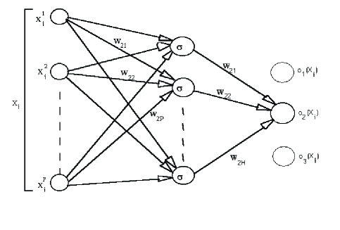
Figure 1: A multilayer perceptron with one hidden layer

Here $a$ is the input to each unit, $o$ is its output and $w_{ij}$ is the weight associated to the connection between units $i$ and $j;$ each unit is defined by two indexes, a superscript specifying its layer (i.e. input, hidden or output layer) and a subscript labelling each unit in a layer.
The training procedure is finalized to find the best set of weights $\{w_{ij}\}$ solving the approximation problem $o\left(x_{i}\right)\approx F\left(x_{i}\right)$ and this is usually reached by the iterative process corresponding to the standard backpropagation algorithm.

At each step, each weight is modified accordingly to the gradient descent rule (a more detailed description can be found in rum ), completed with the momentum term, $w_{ij}=w_{ij}+\Delta w_{ij}$, $\Delta w_{ij}=-\eta\frac{\partial E}{\partial w_{ij}}$ where $E$ is the error functional defined above.
This procedure is iterated many times over the complete set of examples $\{x_{i},F\left(x_{i}\right)\}$ (the training set), and under appropriate conditions it converges to a suitable set of weights defining the desired approximating function. Convergence is usually defined in terms of the error functional, evaluated over the whole training set; when a pre-selected threshold $E_{T}$ is reached, the NN can be tested using a different set of data $\{x_{i}^{\prime},F\left(x_{i}^{\prime}\right)\}$, the so called test set.

4 Data processing and results

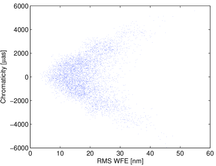
Figure 2: Distribution of chromaticity vs. RMS WFE over the test set.

In this section we describe the identification of the most convenient image parameters, the generation of the training and test sets, and the results from the NN processing. The sources are represented by the monochromatic PSF at the wavelength of respectively 628 nm (B3V) and 756 nm (M8V), deduced from the blackbody spectrum associated to the effective temperature of each star, and the expected spectral distributions of instrument transmission and quantum efficiency.

4.1 Aberration sample

In order to investigate the relationship among image moments and chromaticity, we start from a reasonable sampling of the aberration space, using a uniform random distribution of the 21 lowest order Zernike coefficients (Tab 1), within the range $\pm 50$ nm on each term.
For each aberration case, defined by the set of 21 Zernike coefficient values, we evaluate the RMS WFE for verification purposes and we build the PSF for the two source cases; on the PSF, the photo-centre position is evaluated as the COG, and the moments up to order five are computed accordingly to the definitions in Eq. (4), after across scan integration to replicate the Gaia measurement process. The chromaticity is directly derived as COG difference.
In Fig.2 we show the distribution of chromaticity vs. RMS WFE over the test set (5821 instances). At increasing values of the aberration RMS WFE, the chromaticity has usually larger absolute value, but the relationship is not simple; the same consideration holds for the relationship between chromaticity and any other image moment, due to diffraction non-linearity. Some statistical parameters of the distribution of chromaticity and WFE values in the training data set are listed in Tab. 2.

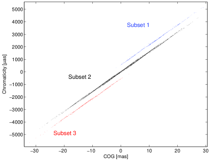
Figure 3: Distribution of chromaticity vs. image COG over the test set.

The average RMS WFE corresponds to an overall optical quality of about $\lambda$/30 at 600 nm, i.e. a comparably good performance; some of the optical designs considered for Gaia provide a RMS WFE of about 40 nm, or $\lambda$/15 at 600 nm. The chromaticity evaluated on the proposed designs has peak values of $\sim 2-3$ mas, localised in specific field positions, and symmetric distribution for the nominal aligned configuration. The random data set considered is thus reasonably representative of a range of realistic optical configurations.

	Chromaticity	RMS WFE
	[$\mu$as]	[nm]
Min.	-5289.3	2.99
Mean	6.1	18.71
Max.	5365.9	46.26
RMS	1648.2	6.81

Table 2: Statistics over the training data set of chromaticity and RMS WFE.

4.2 Neural network input

We verify that the across scan moments ($x$ in the Gaia reference frame) are all irrelevant, i.e. their effect on chromaticity is negligible. Usage of the standard one-dimensional science data is therefore appropriate, without operation changes. The moments are all computed with straightforward operations from the measured data, as well as the variation with respect to the nominal moment values of a selected reference spectral type.
Some of the along scan ($y$) moments do not show an apparent signature associated to chromaticity. A few of them are still required to provide an acceptable description of the image profile: the moment selection was verified on the NN, removing some of them until reaching the minimum number of parameters compatible with good convergence of the training.

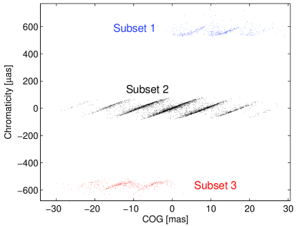
Figure 4: Distribution of residual chromaticity vs. image COG, after slope subtraction.

From the data distribution, it appears that some pre-processing is recommended, in order to ease the subsequent neural processing. This is most apparent in the distribution of chromaticity with respect to the nominal image COG, shown in Fig.3 for the test set. The data points are distributed in three well-defined regions following parallel straight lines, shown in figure by different colours.
The chromaticity / COG structure is shown with even more clarity by subtracting the average slope, derived by linear fit on the central peak of the distribution. The fit parameters are: 157.83 $\mu as/mas$ (slope); 0.06 $\mu as$ (offset). In Fig.4 we show the distribution of the chromaticity residuals after subtraction of the above straight line. The number of data instances in each side peak is about 9% of the sample. The peaks are quite symmetric and corresponding to $\pm 600\ \mu$as. From the residuals, a finer structure appears, which is not currently used in pre-processing.

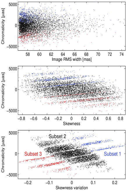
Figure 5: Distribution of chromaticity vs. image RMS width (top), skewness (centre) and skewness variation (bottom).

The classification of data instances in the chromaticity/COG groups (subsets 1, 2 and 3) is taken into account in evaluating the distribution of chromaticity vs. other moments. In some of the plots, the groups are clearly localised in specific parameter regions. Besides, the structure is more complex.

Taking advantage of the structure identified on the COG distribution, we show in Fig. 5 the distribution of chromaticity vs. image RMS width (top panel), skewness (central panel), and skewness variation (bottom panel) between the selected blue and red stars. The subsets are shown here with the same colours as in Fig. 3 and 4, i.e. blue for subset 1, black for subset 2 and red for subset 3.
The RMS width (top panel) and other even order moments do not show an apparent structure, and most of them are not used in the neural processing.
Odd order moments do not evidence directly the subset structure, as for the skewness, in the central panel of Fig. 5. Besides, the distribution of chromaticity vs. skewness variation with spectral type (bottom panel) clearly shows clustering of the three subsets. This appears a convenient choice for NN input, as it carries significant information. Similar effects are shown by other odd order moments.

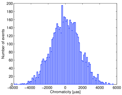
Figure 6: Input chromaticity distribution.

The NN input can therefore be defined in terms of the local instrument response, encoded in the nominal moments for a reference star, and the individual measurement moments. The COG of the reference object is the deviation of the image position with respect to an ideal system, and it is associated to the classical distortion. The other reference object inputs are the image RMS width, the third and fifth order moments. The inputs associated to the measured signal, from an unknown type star, is a simple pair of values, i.e. the variation in the third and fifth order moments with respect to the known reference case.
Also, taking advantage of the data structure discussed above, we subtract the linear trend to the target (the chromaticity) in the training set. This pre-processing is supposed to ease the NN computational load. The inverse transformation is applied to the output data on the test set.
The training and test sets include respectively the data of 20000 and 5820 aberration instances, built accordingly to the above process. The histogram of input chromaticity distribution in the test set (Fig. 6) is approximately Gaussian.

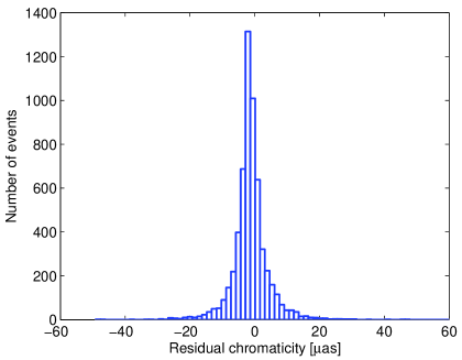
Figure 7: Residual chromaticity distribution.

4.3 Neural processing

We use a sigmoidal NN with six inputs (four nominal and two measured values), one output (the chromaticity), and a single hidden layer with 300 units. The NN is optimised on the training set, and its performance is verified on the test set, as described in Sect. 3.

Chromaticity	Input	Residual
Min. [$\mu$as]	-5975.4	-49.1
Mean [$\mu$as]	19.0	-1.3
Max. [$\mu$as]	5590.8	100.1
RMS [$\mu$as]	1641.8	5.7
Fraction in $\pm 3\sigma[\%]$	99.8	98.0

Table 3: Statistics over the test set of input and residual chromaticity, and fraction of instances within $\pm 3\sigma$.

We use an incremental training, i.e. we split the training set in four subsets of 5000 examples. In the first training phase, the NN is trained by 1000 iterations on the first subset, then we add the second data subset for additional 1000 iterations on the new compound set of 10000 examples, and so on until including the whole training set. The NN training on the complete data set is carried on for a total of 8000 iterations, with monotonic decrease of the internal overall RMS error on the training set.

The NN performance is evaluated on the test set; in particular, the discrepancy between the NN output (estimated chromaticity) and target (actual chromaticity for the test set data instances) can be considered as the residual chromaticity after correction based on the NN results. The residual chromaticity distribution (Fig. 7) is quite symmetric vs. zero, and the main statistical parameters are listed in Tab. 3, compared with the corresponding values in the input test set. We remark that 98% of the output data are within the $\pm 3\sigma$ interval, vs. a corresponding fraction of 99.8% on the input.

Since the goal is the computation of output values coincident with the pre-defined target values, the characteristics, i.e. the relationship between input and output (plot shown in Fig. 8) is ideally a straight line ($y=a+bx$) at angle $\pi/4$, passing for the origin, i.e. with parameters $\{a=0,\ b=1\}$. We compute the best fit parameters of the NN output vs. target distribution and their standard deviation; the results, shown in Tab. 4, are quite consistent with the expectations.

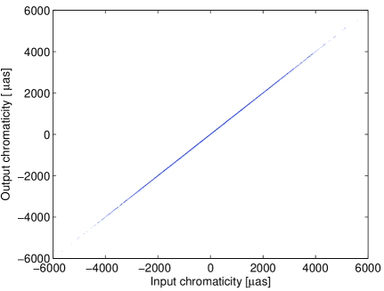
Figure 8: NN performance: input/output characteristics.

Offset	$a=1.30\pm 0.07$
Slope	$b=1.0002\pm 0.5e-4$

Table 4: Linear fit of NN output vs. input chromaticity.

5 Conclusions

In this paper we use a neural network to diagnose and correct the chromaticity on astrometric measurements, in a framework consistent with the mission Gaia. The science data are efficiently encoded in a set of low order image moments. The NN, with 300 internal nodes, is trained on a set of 20,000 data instances, and evaluated on a test set of 5820 cases.

The NN diagnostics on the test set appears to be quite effective, as the RMS residual chromaticity, after correction based on NN results, is reduced by more than two orders of magnitude (factor $\sim 280$) with respect to the initial RMS value (Tab. 3).

Applying the network output for correction of the chromaticity on the elementary Gaia measurements, therefore, we may expect a significant reduction of this source of systematic error; in particular, the residual chromaticity can be expected to be random, and possibly subject to further statistical averaging in subsequent measurements. A word of caution is in order, however, due to the 1.3 $\mu as$ residual offset. This may not be reduced as easily by simple measurements statistics, and it would be desirable that this was close to zero. Besides, it appears that the residual offset is related to the limited size of the training set, and the number of internal nodes, with respect to the large input chromaticity range. Also, it may be related to the mean chromaticity of the training set, close to $6\mu as$ rather than zero.
We expect that, increasing the training set and the number of nodes, the residual chromaticity offset will decrease. This will be part of the future developments. Also, the sensitivity to measurement noise, as propagated to the image moments, will be subject of further investigations.

From the current results, neural network diagnostics for suppression of the chromatic errors on astrometric measurements appears to be a highly promising tool.

References

- (1) [1] Born M., Wolf E., 1985, Principles of optics, Pergamon, New York.
- (2) [2] Cancelliere R., Gai M., 2003, A Comparative Analysis of Neural Network Performances in Astronomy Imaging, Applied Numerical Mathematics, vol. 45, n. 1, p. 87.
- (3) [3] Cancelliere R., Gai M., Neural Network Performances in Astronomical Image Processing, Proceedings of the 11th European Symposium on Artificial Neural Networks ESANN’2003, Bruges (Belgium), 23-25/4/2003, p.515.
- (4) [4] Gai M., Casertano S., Carollo D., Lattanzi M.G., 1998, Location estimators for interferometric fringe, Publ. Astron. Soc. Pac., 110, p. 848.
- (5) [5] Gai M., Carollo D., Delbó M., Lattanzi M.G., Massone G., Bertinetto F., Mana G., Cesare S., 2001, Location accuracy limitations for CCD cameras, A&A 367, p. 362.
- (6) [6] Haykin S., 1994, Neural Networks, a Comprehensive Foundation, IEEE Computer Society Press.
- (7) [7] Loyd-Hart M. et al., 1992, First Results of an On-line Adaptive Optics System with Atmospheric Wavefront Sensing by an Artificial Neural Network, ApJ, vol. 390, p. L41.
- (8) [8] Minsky M., Papert S., 1969, Perceptrons, Cambridge, MA:MIT Press.
- (9) [9] Perryman M.A.C. et al., GAIA - Composition, formation and evolution of the galaxy. Concept and technology study, Rep. and Exec. Summary, ESA-SCI(2000)4, European Space Agency, Munich, Germany, 2000.
- (10) [10] Rumelhart D., Hinton G.E., Williams R.J., 1986, Learning internal representation by error propagation, in Parallel Distribuited Processing (PDP): Exploration in the Microstructure of Cognition, MIT Press, Cambridge, Massachussetts, vol. 1, p. 318.
- (11) [11] Wizinowich P., Loyd-Hart M., Angel R., 1991, Adaptive Optics for Array Telescopes Using Neural Networks Techniques on Transputers, Transputing ’91, IOS Press, Washington D.C., vol. 1, p. 170.