Stochastical distributions of lens and source properties for observed galactic microlensing events

Abstract

A comprehensive new approach is presented for deriving probability densities of physical properties characterizing the lens and source that constitute an observed galactic microlensing event. While previously encountered problems are overcome, constraints from event anomalies and model parameter uncertainties can be incorporated into the estimates. Probability densities for given events need to be carefully distinguished from the statistical distribution of the same parameters among the underlying population from which the actual lenses and sources are drawn. Using given model distributions of the mass spectrum, the mass density, and the velocity distribution of Galactic disk and bulge constituents, probability densities of lens mass, distance, and the effective lens-source velocities are derived, where the effect on the distribution that arises from additional observations of annual parallax or finite-source effects, or the absence of significant effects, is shown. The presented formalism can also be used to calculate probabilities for the lens to belong to one or another population and to estimate parameters that characterize anomalies. Finally, it is shown how detection efficiency maps for binary-lens companions in the physical parameters companion mass and orbital semi-major axis arise from values determined for the mass ratio and dimensionless projected separation parameter, including the deprojection of the orbital motion for elliptical orbits. Compared to the naive estimate based on ’typical values’, the detection efficiency for low-mass companions is increased by mixing in higher detection efficiencies for smaller mass ratios (i.e smaller masses of the primary).

1 Introduction

During the recent years, more than 2000 microlensing events have been observed and corresponding model parameters have been published. However, these model parameters in general do not coincide with the underlying physical characteristics of lens and source star, which are their distances from the observer, $D_{\mathrm{L}}$ and $D_{\mathrm{S}}$, respectively, the mass $M$ of the lens, and the relative proper motion $\mu_{\mathrm{LS}}$ between lens and source. For ’ordinary’ events, compatible with rectilinear motion between point-like sources and lenses, the only parameter related to these characteristics is the event time-scale $t_{\mathrm{E}}=\theta_{\mathrm{E}}/\mu_{\mathrm{LS}}$, which corresponds to the time in which the source moves by the angular Einstein radius

$$\theta_{\mathrm{E}}=\sqrt{\frac{4GM}{c^{2}}\,\frac{D_{\mathrm{S}}-D_{\mathrm{L}}}{D_{\mathrm{L}}\,D_{\mathrm{S}}}}=\sqrt{\frac{4GM}{c^{2}}\,\frac{\pi_{\mathrm{LS}}}{1~{}\mathrm{AU}}}$$ (1)

relative to the lens, where $\pi_{\mathrm{LS}}=1~{}\mathrm{AU}\,(D_{\mathrm{L}}^{-1}-D_{\mathrm{S}}^{-1})$ denotes the relative lens-source parallax.

With the physical lens characteristics being statistically distributed according to the mass density and velocity distribution of lenses and sources as well as the mass spectrum of the lenses, the distribution of observed parameters in the ensemble of galactic microlensing events can be used to measure these distributions. De Rùjula, Jetzer & Massó (1991) have shown explicitly how statistical moments of the observed time-scale distributions translate into moments of the underlying mass spectrum of the lenses.

A different question is posed by asking for the stochastical distribution of physical lens and source properties given the observed model parameters for a single realized event. In the literature, this distinction has frequently not been made strictly enough, leading to some confusion. In particular, the probability density of the lens mass averaged over all observed events does not converge to the underlying mass spectrum. By quoting a probability for the lens mass in a given event to assume a specific value, De Rùjula et al. (1991) did not produce a meaningful result, since the probability for any random variable to assume a specific value is zero. Further common misconceptions exist around a ’relative probability’, which is not defined, and a ’most-probable value’, which does not exist either. A finite probability can only be attached to a finite interval of values, given as the integral over the probability density of the considered quantity. Dominik (1998a) realized that in order to derive information about the lens mass and other properties for a given event, one is dealing with a probability density, which carries the inverse dimension of the quantity it refers to, rather than a likelihood (e.g. Alcock et al., 1995). In fact, likelihood functions and probability densities are different entities, which can be seen explicitly from the following property: If a likelihood for a quantity $a$ has a maximum at some value $a_{0}$, the likelihood for any function $f(a)$ of the quantity $a$ has a maximum at $f(a_{0})$, whereas such a property does not hold for probability densities, i.e. $\left\langle f(a)\right\rangle\neq f(\left\langle a\right\rangle)$ may occur, where $\left\langle a\right\rangle$ denotes the expectation value of $a$. However, like De Rùjula et al. (1991) before, Dominik (1998a) still failed to realize that a statistical mass spectrum of the lens population needs to be assumed along with the space- and velocity-distributions of lenses and sources. Moreover, confusions around the ill assumption of a fixed-mass spectrum $\propto\delta(M-M_{\mathrm{fixed}})$ led to incorrect results for power-law mass spectra, where the power-law index would have to be shifted by unity in order to obtain correct expressions. For determining the event characteristics of MACHO 1997-BLG-41, Albrow et al. (2000a) used a discretization of the statistical distributions of the basic lens and source properties in the form of a Monte-Carlo simulation, which is a variant of the approach of Dominik (1998a). Some of the related ideas have been further developed into a related formalism arguing on the basis of Bayesian statistics used in the analysis of OGLE 2003-BLG-423 (Yoo et al., 2004), where the Galaxy model is used as the prior for the model parameters.

In this paper, a revised comprehensive framework is presented for combining the model parameters as determined from the observations with Galaxy models in order to estimate physical lens and source properties for a given event. This refined approach overcomes the previously encountered problems and allows the inclusion of model constraints from event anomalies as well as model parameter uncertainties. Moreover, by considering different lens populations, a probability that the observed event with its parameters results from one or the other is obtained, which is taken into account for deriving the probability densities of the event characteristics. Rather than having to rely on Monte-Carlo simulations, all results are obtained in the form of closed expressions by means of integrals over the statistical distributions of the lens and source properties.

In Sect. 2, the role of the event rate for deriving the desired probability densities of lens and source properties is discussed, while Sect. 3 looks at the global properties of the ensemble of microlensing events such as the distribution of the event time-scale and the contribution arising from different lens populations. The probability densities of key properties of the lens, namely its mass, distance, and relative velocity with regard to a source at rest, that follow from a measurement of the event time-scale and the Galaxy model are derived and discussed in Sect. 4, whereas Sect. 5 focusses on the implications if further constraints arise either from the measurement or from upper limits on additional model parameters, where the two cases of annual parallax and finite source size are considered explicitly in detail. Sect. 6 then discusses probability densities of further quantities such as the parallax and finite-source parameters as well as the orbital semi-major axis and orbital period for binary lenses, before Sect. 7 shows how the presented approach can be used to determine the detection efficiency for companions (such as planets) to the lens star as function of the physical properties of the system. Sect. 8 finally provides a summary. The underlying probabilistic approach is presented in Appendix A, details of the adopted Galaxy model can be found in Appendix B, and Appendix C discusses the statistics of the orbits of binary systems and in particular the projection factor between the actual angular separation and the semi-major axis.

2 Properties determining microlensing events

Microlensing relies on the chance alignment of observed source stars with intervening massive objects acting as lenses, where the degree of alignment is characterized by the angular Einstein radius as defined by Eq. (1), which depends on the lens mass $M$ as well as on the source distance $D_{\mathrm{S}}$ and the lens distance $D_{\mathrm{L}}$. With a two-dimensional angular separation $\mn@boldsymbol{\theta}$ between lens and source, the magnification of the source star caused by the gravitational field of the lens in general depends only on $\mn@boldsymbol{u}=\mn@boldsymbol{\theta}/\theta_{\mathrm{E}}$, while for a point source it even depends on its absolute value $u=|\mn@boldsymbol{u}|$ only, taking the analytical form (e.g. Paczyński, 1986)

$$A(u)=\frac{u^{2}+2}{u\,\sqrt{u^{2}+4}}\,.$$ (2)

The basic properties of point-like lenses and sources that affect the microlensing light curve are the source magnitude $m_{\mathrm{S}}$, the source distance $D_{\mathrm{S}}$, the lens mass $M$, the lens distance $D_{\mathrm{L}}$, the relative proper motion between lens and source $\mu_{\mathrm{LS}}$, taking into account the motion of the observer, and the blend magnitude $m_{\mathrm{B}}$. If one considers the source distance $D_{\mathrm{S}}$ as well-constrained (there is no problem of including an uncertainty on this parameter as well), and uses the fact that there is no correlation between lens properties and the source or the blend magnitude, it is sufficient to consider lens mass $M$, lens distance $D_{\mathrm{L}}$ and proper motion $\mu_{\mathrm{LS}}$ as the descriptive properties for a given microlensing event. A binary lens involves further characteristics, namely its mass ratio $q$ and 6 orbital elements that can be chosen as the semi-major axis $a$, the eccentricity $e$, three parameters describing the orientation of the orbit (such as the inclination, the longitude of the ascending node, and the argument of perihelion), and finally an orbital phase (such as the mean anomaly at a given epoch). Distributions of the mass ratio $q$, the semi-major axis $a$, and the eccentricity $e$ are pairwise correlated and also depend on the total mass $M$ of the system and the actual types of stars involved, where our current knowledge on these is rather limited.

Let $v=D_{\mathrm{L}}\,\mu_{\mathrm{LS}}$ denote the effective velocity at the lens distance that corresponds to the proper motion $\mu_{\mathrm{LS}}$, while the Einstein radius $r_{\mathrm{E}}=D_{\mathrm{L}}\,\theta_{\mathrm{E}}$ is the physical size of the angular Einstein radius $\theta_{\mathrm{E}}$ at this distance. With the mass spectrum $\Phi_{M}(M)$ and the effective transverse velocity $v$ being distributed as $\Phi_{v}(v)$, the contribution to the event rate by lenses in an infinitely thin sheet at distance $D_{\mathrm{L}}$ with masses in the range $[M,M+dM]$ and velocities in the range $[v,v+dv]$ is given by

$$\mathrm{d}\Gamma=w_{0}\,\frac{\rho(D_{\mathrm{L}})}{M}\,\Phi_{M}(M)\,v\,\Phi_{v}(v)\,r_{\mathrm{E}}\,\mathrm{d}M\,\mathrm{d}v\,\mathrm{d}D_{\mathrm{L}}\,,$$ (3)

where $\rho(D_{\mathrm{L}})$ is the volume mass density, so that the differential area number density reads

$$\mathrm{d}n=\frac{\rho(D_{\mathrm{L}})}{M}\,\Phi_{M}(M)\,\mathrm{d}M\,\mathrm{d}D_{\mathrm{L}}\,,$$ (4)

and $w_{0}$ is a dimensionless factor representing a characteristic width that defines the range of impact parameters for which a microlensing event is considered to occur. Commonly, an ’event’ is defined to take place if the source happens to be magnified by more than an adopted threshold value $A_{\mathrm{T}}$, i.e. $A\geq A_{\mathrm{T}}$, where the choice $A_{\mathrm{T}}=3/\sqrt{5}\approx 1.34$ corresponds to $u_{\mathrm{T}}=1$, according to Eq. (2), which means that the source passes within the angular Einstein radius of the lens, and therefore $w_{0}=2$.

Instead of $D_{\mathrm{L}}$, let us use the dimensionless fractional distance $x\equiv D_{\mathrm{L}}/D_{\mathrm{S}}$, which is distributed as $\Phi_{x}(x)=D_{\mathrm{S}}\,\rho(xD_{\mathrm{S}})/\Sigma$, with $\Sigma=\int_{0}^{D_{\mathrm{S}}}\rho(D_{\mathrm{L}})\,\mathrm{d}D_{\mathrm{L}}$ being the total surface mass density. Let us further assume that the mass spectrum $\Phi_{M}(M)$ is not spatially-dependent and involves a minimal mass $M_{\mathrm{min}}$ and a maximal mass $M_{\mathrm{max}}$, while the velocity distribution $\Phi_{v}(v,x)$ depends on the lens (and source) distance. With these definitions and assumptions, the event rate reads

$$\Gamma=w_{0}\,\sqrt{\frac{4G}{c^{2}}}\,D_{\mathrm{S}}^{1/2}\,\Sigma\,\left(\int\limits_{M_{\mathrm{min}}}^{M_{\mathrm{max}}}\frac{\Phi_{M}(M)}{\sqrt{M}}\,\mathrm{d}M\right)\;\times$$

$$\times\;\left(\int\limits_{0}^{1}\int\limits_{0}^{\infty}v\,\Phi_{v}(v,x)\,\mathrm{d}v\,\sqrt{x(1-x)}\,\Phi_{x}(x)\,\mathrm{d}x\right)\,.$$ (5)

As discussed in detail in Appendix A, the corresponding weight function

$$\Omega(M,v,x) = w_{0}\,\frac{\Sigma}{M}\,v\,r_{\mathrm{E}}(D_{\mathrm{S}},M,x)$$ (6)

$$= w_{0}\,\sqrt{\frac{4G}{c^{2}}}\,D_{\mathrm{S}}^{1/2}\,\frac{\Sigma}{\sqrt{M}}\,v\,\sqrt{x(1-x)}$$

for the basic system properties $\mn@boldsymbol{a}=(M,v,x)$ provides probability densities for any lens property that can be expressed as function of the basic properties by means of Bayes’ theorem.

By introducing a dimensionless velocity parameter $\zeta=v/v_{\mathrm{c}}$, where $v_{\mathrm{c}}$ denotes a characteristic velocity, and with

$$r_{\mathrm{E},\sun}=\sqrt{\frac{GM_{\sun}}{c^{2}}\,D_{\mathrm{S}}}$$ (7)

being the Einstein radius of a solar-mass lens located half-way between observer and source ($x=0.5$), the event rate can be written as

$$\Gamma=\Gamma_{0}\,\left(\int\limits_{M_{\mathrm{min}}/M_{\sun}}^{M_{\mathrm{max}}/M_{\sun}}\frac{\Phi_{M/M_{\sun}}(M/M_{\sun})}{\sqrt{M/M_{\sun}}}\,\mathrm{d}(M/M_{\sun})\right)\;\times$$

$$\times\;\left(\int\limits_{0}^{1}\int\limits_{0}^{\infty}\zeta\,\Phi_{\zeta}(\zeta,x)\,\mathrm{d}\zeta\,\sqrt{x(1-x)}\,\Phi_{x}(x)\,\mathrm{d}x\right)\,,$$ (8)

with $\Gamma_{0}=2\,w_{0}\,r_{\mathrm{E},\sun}\,v_{\mathrm{c}}\,\Sigma$ and the dimensionless distributions $\Phi_{\zeta}(\zeta)=v_{\mathrm{c}}\,\Phi_{v}(v_{\mathrm{c}}\,\zeta)$ and $\Phi_{M/M_{\sun}}(M/M_{\sun})=M_{\sun}\,\Phi_{M}(M)$. With the definition of $\Gamma_{0}$, the weight function takes the form

$$\Omega(M,\zeta,x)=\Gamma_{0}\,\left(M/M_{\sun}\right)^{-1/2}\,\zeta\,\sqrt{x(1-x)}\,.$$ (9)

3 Distribution of properties for the ensemble of events

For ordinary microlensing light curves, i.e. those that can be approximated by lensing of a point-like source star by a single point-mass lens and uniform motion of the lens relative to the line-of-sight from the observer to the source, the only observable that is related to the physical parameters of the system is the time-scale

$$t_{\mathrm{E}}=\theta_{\mathrm{E}}/\mu_{\mathrm{LS}}=\frac{1}{v}\,\sqrt{\frac{4GM}{c^{2}}\,D_{\mathrm{S}}\,x(1-x)}\,,$$ (10)

which thus involves all the basic properties $M$, $v$, and $x$.

For an obtained best-fit estimate $t_{\mathrm{E}}^{(0)}$, let us define

$$\eta_{t_{\mathrm{E}}}^{(0)}=\frac{t_{\mathrm{E}}^{(0)}\,v_{\mathrm{c}}}{r_{\mathrm{E},\sun}}\,,$$ (11)

where $r_{\mathrm{E},\sun}$ is given by Eq. (7). With $\eta_{t_{\mathrm{E}}}^{(0)}$ depending on the basic system properties as $\eta_{t_{\mathrm{E}}}^{(0)}=2\,\sqrt{M/M_{\sun}}\,\sqrt{x(1-x)}/\zeta$, Eq. (76) applied to the expression for the event rate $\Gamma$ as given by Eq. (8) yields the corresponding event rate density as

$$\gamma_{\eta_{t_{\mathrm{E}}}}(\eta_{t_{\mathrm{E}}}^{(0)})=\frac{4\,\Gamma_{0}}{[\eta_{t_{\mathrm{E}}}^{(0)}]^{3}}\,\int\limits_{M_{\mathrm{min}}/M_{\sun}}^{M_{\mathrm{max}}/M_{\sun}}\sqrt{M/M_{\sun}}\;\times$$

$$\times\;\Phi_{M/M_{\sun}}\left(M/M_{\sun}\right)\;\times$$

$$\times\;\int\limits_{0}^{1}\Phi_{\zeta}\left(2\,\sqrt{M/M_{\sun}}\,\sqrt{x(1-x)}/\eta_{t_{\mathrm{E}}}^{(0)},x\right)\;\times$$

$$\times\;[x(1-x)]^{3/2}\,\Phi_{x}(x)\,\mathrm{d}x\,\mathrm{d}(M/M_{\sun})\,,$$ (12)

while $\gamma_{t_{\mathrm{E}}}(t_{\mathrm{E}})=(v_{\mathrm{c}}/r_{\mathrm{E},\sun})\,\gamma_{\eta_{t_{\mathrm{E}}}}[(t_{\mathrm{E}}\,v_{\mathrm{c}})/r_{\mathrm{E},\sun}]$ is the corresponding density of $t_{\mathrm{E}}$, and ${\hat{\gamma}}_{t_{\mathrm{E}}}=\gamma_{t_{\mathrm{E}}}/\Gamma$ gives the distribution of event time-scales arising from the lens population.

If the lens may belong to one or another population with different mass spectra, mass densities, and velocity distributions, the event rate density $\gamma_{t_{\mathrm{E}}}(t_{\mathrm{E}}^{(0)})$ for the observed event time-scale $t_{\mathrm{E}}^{(0)}$ provides a means to decide to which population the lens objects belongs. Namely, the probability for the lens to be drawn from each of the populations is proportional to the corresponding event rate density. Since the event rate density is proportional to the surface mass density along the line-of-sight, conclusions about the latter can be drawn, e.g. a likelihood for a certain surface mass density can be obtained on the assumption that the lens in the considered event with time-scale $t_{\mathrm{E}}^{(0)}$ (or possible additional observables) belongs to a chosen population. Such considerations are of special interest with regard to the mass content of the Galactic halo and the still open question what fraction of the observed microlensing events in the direction of the Magellanic Clouds is caused by lenses in the Magellanic Clouds themselves (e.g Sahu & Sahu, 1998; Gyuk et al., 2000; Mancini et al., 2004).

For a source located in the Galactic bulge, namely in the direction of Baade’s window with $(l,b)=(1\degr,-3.9\degr)$ at a distance of $D_{\mathrm{S}}=8.5~{}\mathrm{kpc}$ and the lens residing in the Galactic disk or bulge, Fig. 1 shows the distribution of time-scales and lens masses including the contributions of the individual lens populations, while Fig. 2 shows the fractional contributions $\kappa_{t_{\mathrm{E}}}(t_{\mathrm{E}})$ of disk or bulge lenses as function of the observed event time-scale $t_{\mathrm{E}}^{(0)}$, where $\kappa_{t_{\mathrm{E}}}^{\mathrm{disk}}=\gamma_{t_{\mathrm{E}}}^{\mathrm{disk}}/(\gamma_{t_{\mathrm{E}}}^{\mathrm{disk}}+\gamma_{t_{\mathrm{E}}}^{\mathrm{bulge}})$, $\kappa_{t_{\mathrm{E}}}^{\mathrm{bulge}}=\gamma_{t_{\mathrm{E}}}^{\mathrm{bulge}}/(\gamma_{t_{\mathrm{E}}}^{\mathrm{disk}}+\gamma_{t_{\mathrm{E}}}^{\mathrm{bulge}})$, and $\gamma_{t_{\mathrm{E}}}(t_{\mathrm{E}})$ is given by Eq. (76). Table 1 lists the fractional contributions $\kappa_{t_{\mathrm{E}}}^{\mathrm{disk}}$ and $\kappa_{t_{\mathrm{E}}}^{\mathrm{bulge}}$ for selected time-scales. All details of the assumed mass spectra, mass densities, and velocity distributions for the underlying populations can be found in Appendix B. Among all created events, 35 per cent are caused by lenses in the Galactic disk and 65 per cent by lenses in the Galactic bulge. Only for timescales $t_{\mathrm{E}}\la 2~{}\mathrm{d}$, disk lenses provide a significantly larger contribution than bulge lenses, whereas the latter dominate for $2~{}\mathrm{d}\la t_{\mathrm{E}}\la 40~{}\mathrm{d}$ and for $t_{\mathrm{E}}\ga 100~{}\mathrm{d}$. For $40~{}\mathrm{d}\la t_{\mathrm{E}}\la 100~{}\mathrm{d}$, both populations yield comparable contributions. One finds a median time-scale $t_{\mathrm{E}}\sim 18~{}\mathrm{d}$, or $t_{\mathrm{E}}\sim 17~{}\mathrm{d}$ for bulge and $t_{\mathrm{E}}\sim 24~{}\mathrm{d}$ for disk lenses. The distribution of ${\hat{\gamma}}_{t_{\mathrm{E}}}$ does not properly reflect that of the time-scales observed by the experiments, since their sensitivity for detecting an event depends on the event duration. In particular, a significant fraction of events with short time-scales is missed with a roughly daily sampling. The median mass is $0.32~{}M_{\sun}$, with about 1/3 of the events caused by lenses more massive than $0.5~{}M_{\sun}$, and about 1/5 by lenses heavier than $0.8~{}M_{\sun}$.

Figure 1: Distribution of event time-scales $t_{\mathrm{E}}$ and lens masses among all created microlensing events for a source located in the Galactic bulge at $D_{\mathrm{S}}=8.5~{}\mathrm{kpc}$ in the direction of Baade’s window $(l,b)=(1\degr,-3.9\degr)$ with the individual contributions of disk and bulge lenses. Details of the adopted Galaxy model can be found in Appendix B.

Figure 2: Fractional contributions $\kappa_{t_{\mathrm{E}}}^{\mathrm{disk}}$ and $\kappa_{t_{\mathrm{E}}}^{\mathrm{bulge}}$ to the event rate density $\gamma_{t_{\mathrm{E}}}(t_{\mathrm{E}})$ as a function of the time-scale $t_{\mathrm{E}}$ of an observed event. For a few specific $t_{\mathrm{E}}$, the resulting values of $\kappa_{t_{\mathrm{E}}}^{\mathrm{disk}}$ and $\kappa_{t_{\mathrm{E}}}^{\mathrm{bulge}}$ are listed in Table 1. The source is located in the Galactic bulge at $D_{\mathrm{S}}=8.5~{}\mathrm{kpc}$ in the direction of Baade’s window $(l,b)=(1\degr,-3.9\degr)$.

Table 1: Fractional contributions $\kappa_{t_{\mathrm{E}}}^{\mathrm{disk}}$ and $\kappa_{t_{\mathrm{E}}}^{\mathrm{bulge}}$ of disk or bulge lenses to the event rate density $\gamma_{t_{\mathrm{E}}}(t_{\mathrm{E}})$ of a Galactic bulge source at $D_{\mathrm{S}}=8.5~{}\mathrm{kpc}$ in the direction of Baade’s window by lenses in the Galactic disk or bulge, respectively, for selected event time-scales $t_{\mathrm{E}}$.

$t_{\mathrm{E}}/(1~{}\mathrm{d})$	$\kappa_{t_{\mathrm{E}}}^{\mathrm{disk}}$	$\kappa_{t_{\mathrm{E}}}^{\mathrm{bulge}}$
5	0.25	0.75
10	0.24	0.76
20	0.35	0.65
40	0.50	0.50
80	0.52	0.48

$\kappa_{t_{\mathrm{E}}}^{\mathrm{disk}}=\gamma_{t_{\mathrm{E}}}^{\mathrm{disk}}/(\gamma_{t_{\mathrm{E}}}^{\mathrm{disk}}+\gamma_{t_{\mathrm{E}}}^{\mathrm{bulge}})$ and $\kappa_{t_{\mathrm{E}}}^{\mathrm{bulge}}=\gamma_{t_{\mathrm{E}}}^{\mathrm{bulge}}/(\gamma_{t_{\mathrm{E}}}^{\mathrm{disk}}+\gamma_{t_{\mathrm{E}}}^{\mathrm{bulge}})$, where $\gamma_{t_{\mathrm{E}}}$ is defined by Eq. (76) and can be calculated by means of Eq. (12).

4 Probability densities of system properties for ordinary events

4.1 Lens mass

Let us define $\mu_{0}=M/M_{0}$, where the characteristic mass $M_{0}$ is assumed for the velocity $v_{\mathrm{c}}$ and the lens being located half-way between observer and source ($x=0.5$). Hence, with $\eta_{t_{\mathrm{E}}}^{(0)}$ as defined by Eq. (11), $M_{0}=[\eta_{t_{\mathrm{E}}}^{(0)}]^{2}\,M_{\sun}$, while $\mu_{0}^{\mathrm{min}}=[\eta_{t_{\mathrm{E}}}^{(0)}]^{-2}M_{\mathrm{min}}/M_{\sun}$ and $\mu_{0}^{\mathrm{max}}=[\eta_{t_{\mathrm{E}}}^{(0)}]^{-2}M_{\mathrm{max}}/M_{\sun}$.

With $\mu_{0}$ being related to the basic properties as $\mu_{0}=[\eta_{t_{\mathrm{E}}}^{(0)}]^{-2}(M/M_{\sun})$, one easily finds with Eqs. (86) and (12) the probability density of $\mu_{0}$ for an event with measured $t_{\mathrm{E}}^{(0)}$ to be

$$p_{\mu_{0}}^{(0)}(\mu_{0};\eta_{t_{\mathrm{E}}}^{(0)})=\frac{4\,\Gamma_{0}}{\gamma_{\eta_{t_{\mathrm{E}}}}(\eta_{t_{\mathrm{E}}}^{(0)})}\,\sqrt{\mu_{0}}\;\Phi_{M/M_{\sun}}\left(\mu_{0}\left[\eta_{t_{\mathrm{E}}}^{(0)}\right]^{2}\right)\;\times$$

$$\times\;\int\limits_{0}^{1}\Phi_{\zeta}\left(2\,\sqrt{\mu_{0}\,x(1-x)},x\right)\,[x(1-x)]^{3/2}\,\Phi_{x}(x)\,\mathrm{d}x\,.$$ (13)

Figure 3: Probability density of the lens mass $M$ for selected observed event time-scales $t_{\mathrm{E}}$. With the event rate density $\gamma_{t_{\mathrm{E}}}(t_{\mathrm{E}})$, the relative contributions by disk or bulge lenses are $\kappa_{t_{\mathrm{E}}}^{\mathrm{disk}}=\gamma_{t_{\mathrm{E}}}^{\mathrm{disk}}/(\gamma_{t_{\mathrm{E}}}^{\mathrm{disk}}+\gamma_{t_{\mathrm{E}}}^{\mathrm{bulge}})$ or $\kappa_{t_{\mathrm{E}}}^{\mathrm{bulge}}=\gamma_{t_{\mathrm{E}}}^{\mathrm{bulge}}/(\gamma_{t_{\mathrm{E}}}^{\mathrm{disk}}+\gamma_{t_{\mathrm{E}}}^{\mathrm{bulge}})$, respectively. The figures show the contributions $\kappa_{t_{\mathrm{E}}}\;p_{\lg(M/M_{\sun})}$ of each population along with the total probability density $p_{\lg(M/M_{\sun})}$ of $\lg(M/M_{\sun})$. For the chosen values of $t_{\mathrm{E}}$, the corresponding fractional contributions $\kappa_{t_{\mathrm{E}}}(t_{\mathrm{E}})$ are listed in Table 1.

By means of Eq. (87), the distribution for a fuzzy value of $t_{\mathrm{E}}^{(0)}$ then follows with $p_{\mu_{0}}(\mu_{0};\eta_{t_{\mathrm{E}}}^{(0)})$ being evaluated for every corresponding $\eta_{t_{\mathrm{E}}}^{(0)}$. Frequently, it is more adequate to represent the lens mass on a logarithmic scale. The probability density of $\lg(M/M_{\sun})$ simply follows as

$$p_{\lg(M/M_{\sun})}(\lg(M/M_{\sun}),\eta_{t_{\mathrm{E}}}^{(0)})$$

$$=\;\left[\eta_{t_{\mathrm{E}}}^{(0)}\right]^{-2}\,\frac{M}{M_{\sun}}\,\ln 10\;p_{\mu_{0}}\left(\left[\eta_{t_{\mathrm{E}}}^{(0)}\right]^{-2}\,\frac{M}{M_{\sun}}\right)\,.$$ (14)

For a source located at $D_{\mathrm{S}}=8.5~{}\mathrm{kpc}$ in the direction of Baade’s window with $(l,b)=(1\degr,-3.9\degr)$ as used in the previous section and the lens residing in the Galactic disk or bulge with the Galaxy model described in Appendix B, Fig. 3 shows the mass probability density $p_{\lg(M/M_{\sun})}$ of $\lg(M/M_{\sun})$ for selected values of the observed event time-scale $t_{\mathrm{E}}^{(0)}$. In addition to the resulting $p_{\lg(M/M_{\sun})}$ from both possible lens populations, their individual contributions $\kappa_{t_{\mathrm{E}}}^{\mathrm{disk}}\;p^{\mathrm{disk}}_{\lg(M/M_{\sun})}$ and $\kappa_{t_{\mathrm{E}}}^{\mathrm{bulge}}\;p^{\mathrm{bulge}}_{\lg(M/M_{\sun})}$ are shown, where the factors are determined by the event rate density $\gamma_{t_{\mathrm{E}}}(t_{\mathrm{E}})$ as $\kappa_{t_{\mathrm{E}}}^{\mathrm{disk}}=\gamma_{t_{\mathrm{E}}}^{\mathrm{disk}}/(\gamma_{t_{\mathrm{E}}}^{\mathrm{disk}}+\gamma_{t_{\mathrm{E}}}^{\mathrm{bulge}})$ and $\kappa_{t_{\mathrm{E}}}^{\mathrm{bulge}}=\gamma_{t_{\mathrm{E}}}^{\mathrm{bulge}}/(\gamma_{t_{\mathrm{E}}}^{\mathrm{disk}}+\gamma_{t_{\mathrm{E}}}^{\mathrm{bulge}})$. The fractional contributions $\kappa_{t_{\mathrm{E}}}(t_{\mathrm{E}}^{(0)})$ for the chosen values of $t_{\mathrm{E}}^{(0)}$ are also listed in Table 1. If the uncertainty in $t_{\mathrm{E}}$ is less than 20 per cent, it does not have a significant effect on the probability density.

Table 2: Expectation value and standard deviation for $\lg(M/M_{\sun})$, $x$, and $\lg\zeta$ for selected values of the event time-scale $t_{\mathrm{E}}$.

$t_{\mathrm{E}}/(1~{}\mathrm{d})$	$\left\langle\lg(M/M_{\sun})\right\rangle$	$\sigma_{\lg(M/M_{\sun})}$	${\hat{M}}/M_{\sun}$	$\varsigma_{M/{\hat{M}}}$	$\left\langle x\right\rangle$	$\sigma_{x}$	$\left\langle\lg\zeta\right\rangle$	$\sigma_{\lg\zeta}$	${\hat{v}}/(100~{}\mathrm{km}\,\mathrm{s}^{-1})$	$\varsigma_{v/{\hat{v}}}$
5	-0.95	0.39	0.11	2.4	0.88	0.10	0.42	0.15	260	1.4
10	-0.70	0.37	0.20	2.3	0.83	0.12	0.33	0.16	216	1.4
20	-0.45	0.39	0.36	2.5	0.77	0.15	0.21	0.17	161	1.5
40	-0.18	0.46	0.65	2.9	0.69	0.20	0.07	0.21	117	1.6
80	-0.12	0.58	1.31	3.8	0.63	0.23	-0.07	0.26	84	1.8

In addition to the expectation value $\left\langle\lg(M/M_{\sun})\right\rangle$ and the standard deviation $\sigma_{\lg(M/M_{\sun})}$, the corresponding exponentiated values ${\hat{M}}/M_{\sun}=\exp_{10}[\left\langle\lg(M/M_{\sun})\right\rangle]$ and $\varsigma_{M/{\hat{M}}}=\exp_{10}[\sigma_{\lg(M/M_{\sun})}]$ are listed. Similarly, ${\hat{v}}=\exp_{10}[\left\langle\lg\zeta\right\rangle]\,v_{\mathrm{c}}$ and $\varsigma_{v/{\hat{v}}}=\exp_{10}[\sigma_{\lg\zeta}]$ are given. The source has been assumed to reside in the Galactic bulge at a distance $D_{\mathrm{S}}=8.5~{}\mathrm{kpc}$ in the direction of Baade’s window $(l,b)=(1\degr,-3.9\degr)$ and the Galaxy model described in Appendix B has been adopted. None of the listed values changes significantly if a 20 per cent uncertainty in $t_{\mathrm{E}}$ is considered, where the distributions widen by less than 2 per cent, while mass and velocity estimate shift by less than 0.7 per cent, and the fractional distance $x$ shifts by less than $0.002$.

For the previously chosen selected values of $t_{\mathrm{E}}^{(0)}$, $\left\langle\lg(M/M_{\sun})\right\rangle$ and $\sigma_{\lg(M/M_{\sun})}$ and as well as their exponentiated values are listed in Table 2, while the top panel of Fig. 5 shows these values as a function of $t_{\mathrm{E}}$. While a mass $M\sim 0.36~{}M_{\sun}$ for $t_{\mathrm{E}}^{(0)}=20~{}\mathrm{d}$ is in rough agreement with estimates using a ’typical’ fractional lens distance $x$ and transverse velocity $v$, the assumed mass spectrum with a low abundance for $M\ga 1~{}M_{\sun}$ forces the expected mass to be more narrowly distributed with $t_{\mathrm{E}}$ rather than to follow the naive $M\propto t_{\mathrm{E}}^{2}$ law. In particular, the mass ${\hat{M}}=\exp_{10}[\left\langle\lg(M/M_{\sun})\right\rangle]~{}M_{\sun}$ spans only 1.5 decades between $0.09~{}M_{\sun}$ and $3~{}M_{\sun}$ for time-scales $3~{}\mathrm{d}\leq t_{\mathrm{E}}\leq 150~{}\mathrm{d}$, where the inclusion of one standard deviation extends this range to $0.03~{}M_{\sun}\ldots 15~{}M_{\sun}$.

4.2 Lens distance

Similarly to the treatment of the lens mass, one finds the probability density of the fractional lens distance $x$ for an event with observed $t_{\mathrm{E}}^{(0)}$ (and related $\eta_{t_{\mathrm{E}}}^{(0)}$) with Eqs. (86) and (12) as

$$p_{x}^{(0)}(x;\eta_{t_{\mathrm{E}}}^{(0)})=\frac{4\,\Gamma_{0}}{\gamma_{\eta_{t_{\mathrm{E}}}}(\eta_{t_{\mathrm{E}}}^{(0)})}\,[x(1-x)]^{3/2}\,\Phi_{x}(x)\;\times$$

$$\times\;\int\limits_{\mu_{0}^{\mathrm{min}}}^{\mu_{0}^{\mathrm{max}}}\sqrt{\mu_{0}}\,\Phi_{M/M_{\sun}}\left(\mu_{0}\left[\eta_{t_{\mathrm{E}}}^{(0)}\right]^{2}\right)\;\times$$

$$\times\;\Phi_{\zeta}\left(2\,\sqrt{\mu_{0}\,x(1-x)},x\right)\,\mathrm{d}\mu_{0}$$ (15)

or

$$p_{x}^{(0)}(x;\eta_{t_{\mathrm{E}}}^{(0)})=\frac{4\,\Gamma_{0}}{\gamma_{\eta_{t_{\mathrm{E}}}}(\eta_{t_{\mathrm{E}}}^{(0)})\,[\eta_{t_{\mathrm{E}}}^{(0)}]^{3}}\,[x(1-x)]^{3/2}\,\Phi_{x}(x)\;\times$$

$$\times\;\int\limits_{\lg(M_{\mathrm{min}}/M_{\sun})}^{\lg(M_{\mathrm{max}}/M_{\sun})}(M/M_{\sun})^{3/2}\,\Phi_{M/M_{\sun}}\left(M/M_{\sun}\right)\;\times$$

$$\times\;\Phi_{\zeta}\left(2\,\sqrt{M/M_{\sun}}\,\sqrt{x(1-x)}/\eta_{t_{\mathrm{E}}}^{(0)},x\right)\,\mathrm{d}[\lg(M/M_{\sun})]\,.$$ (16)

Figure 4: Probability density of the fractional lens distance $x$ for selected values of the observed event time-scale $t_{\mathrm{E}}$. Similar to Fig. (3), the individual contributions $\kappa_{t_{\mathrm{E}}}\;p_{x}$ of disk and bulge lenses are shown together with the total probability density $p_{x}$, where the relative weight of the two lens populations is listed in Table 1 for the chosen values of $t_{\mathrm{E}}$.

Figure 5: Expectation value and standard deviation for the logarithmic lens mass $\lg(M/M_{\sun})$, the fractional lens distance $x$ and the logarithmic velocity $\lg\zeta$ as function of the event time-scale $t_{\mathrm{E}}$. While the solid lines mark the expectation values, the dashed lines limit intervals corresponding to the standard deviation.

Fig. 4 shows the probability density $p_{x}$ of the fractional lens distance for selected time-scales, while the expectation value $\left\langle x\right\rangle$ and the standard deviation $\sigma_{x}$ for different $t_{\mathrm{E}}^{(0)}$ are shown in the middle panel of Fig. 5 as well as in Table 2. As before, the source is assumed to be located in the Galactic bulge at $D_{\mathrm{S}}=8.5~{}\mathrm{kpc}$ in the direction of Baade’s window, and the Galaxy model described in Appendix B has been adopted. Shorter time-scales favour larger fractional lens distances, while longer time-scales prefer the lenses to be closer to the observer, in accordance with the disk population yielding the slightly larger contribution to the event rate density for $40~{}\mathrm{d}\la t_{\mathrm{E}}\la 100~{}\mathrm{d}$, whereas the disk dominates for smaller time-scales unless $t_{\mathrm{E}}\la 2~{}\mathrm{d}$.

4.3 Effective velocity and Einstein radius

Figure 6: Probability density of the velocity for selected values of the observed event time-scale $t_{\mathrm{E}}$. As for Figs. 3 and 4, the individual contributions $\kappa_{t_{\mathrm{E}}}\;p_{\lg\zeta}$ of disk and bulge lenses, with the corresponding weight factors listed in Table 1, are shown together with the total probability density $p_{\lg\zeta}$ of $\lg\zeta$, where $\zeta=v/v_{\mathrm{c}}$ is the dimensionless velocity parameter and $v_{\mathrm{c}}=100~{}\mathrm{km}\,\mathrm{s}^{-1}$ has been adopted.

By eliminating $x$ by means of the delta-function, Eq. (86) yields for the probability density of the velocity parameter $\zeta$ for a fixed $\eta_{t_{\mathrm{E}}}^{(0)}$

$$p_{\zeta}^{(0)}(\zeta;\eta_{t_{\mathrm{E}}}^{(0)})=\frac{\Gamma_{0}}{4\,\gamma_{\eta_{t_{\mathrm{E}}}}(\eta_{t_{\mathrm{E}}}^{(0)})}\;\zeta^{4}\;\times$$

$$\times\;\int\limits_{\mu_{0}^{\mathrm{min}}}^{\mu_{0}^{\mathrm{max}}}\frac{\Theta(\mu_{0}-\zeta^{2})}{\mu_{0}^{2}\,\sqrt{1-\zeta^{2}/\mu_{0}}}\;\Phi_{M/M_{\sun}}\left(\mu_{0}\left[\eta_{t_{\mathrm{E}}}^{(0)}\right]^{2}\right)\;\times$$

$$\times\;\sum\limits_{\pm}\Phi_{\zeta}\left(\zeta,\frac{1}{2}\left(1\pm\sqrt{1-\zeta^{2}/\mu_{0}}\right)\right)\;\times$$

$$\times\;\Phi_{x}\left(\frac{1}{2}\left(1\pm\sqrt{1-\zeta^{2}/\mu_{0}}\right)\right)\,\mathrm{d}\mu_{0}\,.$$ (17)

With ${\hat{x}}=\sqrt{1-\zeta^{2}/\mu_{0}}$, one also finds equivalently

$$p_{\zeta}^{(0)}(\zeta;\eta_{t_{\mathrm{E}}}^{(0)})=\frac{\Gamma_{0}}{2\,\gamma_{\eta_{t_{\mathrm{E}}}}(\eta_{t_{\mathrm{E}}}^{(0)})}\;\zeta^{2}\,\Theta(\mu_{0}^{\mathrm{max}}-\zeta^{2})\;\times$$

$$\times\;\int\limits_{{\hat{x}}^{\mathrm{min}}}^{{\hat{x}}^{\mathrm{max}}}\Phi_{M/M_{\sun}}\left(\frac{\zeta^{2}}{1-{\hat{x}}^{2}}\,\left[\eta_{t_{\mathrm{E}}}^{(0)}\right]^{2}\right)\;\times$$

$$\times\;\sum\limits_{\pm}\Phi_{\zeta}\left(\zeta,\frac{1}{2}\left(1\pm\hat{x}\right)\right)\,\Phi_{x}\left(\frac{1}{2}\left(1\pm\hat{x}\right)\right)\,\mathrm{d}{\hat{x}}\,,$$ (18)

where the integration limits are given by

$${\hat{x}}^{\mathrm{min}} = \left\{\begin{array}[]{lcl}\sqrt{1-\zeta^{2}/\mu_{0}^{\mathrm{min}}}&\mathrm{for}&\zeta<\mu_{0}^{\mathrm{min}}\\ 0&\mathrm{for}&\zeta\geq\mu_{0}^{\mathrm{min}}\end{array}\right.\,,$$ (21)

$${\hat{x}}^{\mathrm{max}} = \left\{\begin{array}[]{lcl}\sqrt{1-\zeta^{2}/\mu_{0}^{\mathrm{max}}}&\mathrm{for}&\zeta<\mu_{0}^{\mathrm{max}}\\ 0&\mathrm{for}&\zeta\geq\mu_{0}^{\mathrm{max}}\end{array}\right.\,.$$ (24)

Since $r_{\mathrm{E}}=t_{\mathrm{E}}\,v$, the distribution of the Einstein radius $r_{\mathrm{E}}$ follows that of the velocity $v$ for any value of the event time-scale $t_{\mathrm{E}}$. More precisely, if one defines $r_{\mathrm{E},0}=\eta_{t_{\mathrm{E}}}^{(0)}\,r_{\mathrm{E},\sun}$ as the Einstein radius of the ’typical’ mass $M_{0}$, corresponding to $v=v_{\mathrm{c}}$ and $x=0.5$, one finds that $\rho_{\mathrm{E}}\equiv r_{\mathrm{E}}/r_{\mathrm{E},0}=\zeta$, so that $p_{\rho_{\mathrm{E}}}(\rho_{\mathrm{E}})=p_{\zeta}(\zeta)$.

As for the lens mass $M$ and the fractional lens distance $x\equiv D_{\mathrm{L}}/D_{\mathrm{S}}$, expectation values and standard deviations for the transverse velocity $v=D_{\mathrm{L}}\,\mu=\zeta\,v_{\mathrm{c}}$ at the lens distance are shown in Table 2 for selected time-scales $t_{\mathrm{E}}$, whereas Fig. 6 shows the corresponding probability densities. As before, the source has been assumed to be located in the direction of Baade’s window, at a distance $D_{\mathrm{S}}=8.5~{}\mathrm{kpc}$. The expectation value of $\lg\zeta$ as well as its uncertainty as function of the time-scale $t_{\mathrm{E}}$ is also displayed in the lower panel of Fig. 5.

5 Constraints from parallax and finite-source effects

5.1 Model parameters providing further information

Further information about the lens mass $M$, the fractional lens distance $x$, and the effective velocity parameter $\zeta$ exceeding that provided by the event time-scale $t_{\mathrm{E}}$ can be obtained from events whose light curves are significantly affected by either the annual Earth’s motion around the Sun or the finite size of the observed source star or even both of these effects. Either of these provides an additional relation between $(M,x,\zeta)$ from a model parameter that relates the Einstein radius $r_{\mathrm{E}}(M,x,\zeta)$ to a physical scale which is either the Earth’s orbital radius of $1~{}\mathrm{AU}$ or the radius $R_{\star}$ of the source star.

Moreover, for a binary lens, the total mass arises from the period $P$ and the semi-major axis $a$, so that, as discussed by Dominik (1998b), further information about the lens properties arises from the lens orbital motion. However, it is quite difficult to obtain reliable measurements of the full set of orbital elements in order to determine the period $P$ and the parameter $\rho=a/r_{\mathrm{E}}$, which would provide a relation between $M$, $x$, and $\zeta$. As pointed out in the discussion of the event MACHO 1997-BLG-41 by Albrow et al. (2000a), the lowest-order effects can be attributed to the actual projected differential velocity between the components, which restricts only a subspace with two measured model parameters, while leaving another three undetermined. This strongly limits the power to constrain the lens and source properties. A proper discussion would be quite sophisticated and needs to be tailored to specific cases, so that it exceeds the scope of this paper.

If the light curve is significantly affected by annual parallax resulting from the revolution of the Earth around the Sun, one can determine $\pi_{\mathrm{E}}=\pi_{\mathrm{LS}}/\theta_{\mathrm{E}}$ as a model parameter. In analogy to the definition of $\eta_{t_{\mathrm{E}}}^{(0)}$ by Eq. (11), a corresponding dimensionless parameter reads

$$\eta_{\pi_{\mathrm{E}}^{(0)}} = \frac{2\,\pi_{\mathrm{E}}^{(0)}\,r_{\mathrm{E},\sun}}{1~{}\mathrm{AU}}$$ (25)

$$\approx 2.85\,\pi_{\mathrm{E}}^{(0)}\,\left(\frac{D_{\mathrm{S}}}{1~{}\mathrm{kpc}}\right)^{1/2}\,.$$

Similarly, if the finite size of the source star has a significant effect on the microlensing light curve, the time-scale $t_{\star}=t_{\mathrm{E}}\,[R_{\star}/(D_{\mathrm{S}}\,\theta_{\mathrm{E}})]$, in which the source moves by its own angular radius relative to the lens, can be determined as additional model parameter. Alternatively, one might use a source size parameter $\rho_{\star}=t_{\star}/t_{\mathrm{E}}$ instead. A corresponding dimensionless parameter can be defined as

$$\eta_{t_{\star}^{(0)}} = \frac{2\,t_{\star}^{(0)}\,r_{\mathrm{E},\sun}}{t_{\mathrm{E}}^{(0)}\,R_{\star}}$$ (26)

$$\approx 613\,{\hat{\rho}}_{\star,\sun}\,\left(\frac{D_{\mathrm{S}}}{1~{}\mathrm{kpc}}\right)^{1/2}\,,$$

with the convenient abbreviation ${\hat{\rho}}_{\star,\sun}=(t_{\star}/t_{\mathrm{E}})\,(R_{\star}/R_{\sun})^{-1}$, where $R_{\sun}\approx 6.96\times 10^{5}~{}\mathrm{km}$ denotes the solar radius.

5.2 Parallax

From the expression for the event rate density for an observed $t_{\mathrm{E}}^{(0)}$ and the related $\eta_{t_{\mathrm{E}}}^{(0)}$ as given by Eq. (12), one finds with the additional constraint $\delta[\eta_{\pi_{\mathrm{E}}}^{(0)}-\sqrt{(1-x)/x}\,(M/M_{\sun})^{-1/2}]$ the event rate density in both $\eta_{t_{\mathrm{E}}}^{(0)}$ and $\eta_{\pi_{\mathrm{E}}}^{(0)}$ to be

$$\gamma_{\eta_{t_{\mathrm{E}}},\eta_{\pi_{\mathrm{E}}}}(\eta_{t_{\mathrm{E}}}^{(0)},\eta_{\pi_{\mathrm{E}}}^{(0)})=8\,\Gamma_{0}\,\frac{[\eta_{\pi_{\mathrm{E}}}^{(0)}]^{4}}{[\eta_{t_{\mathrm{E}}}^{(0)}]^{3}}\;\times$$

$$\times\;\int\limits_{M_{\mathrm{min}}/M_{\sun}}^{M_{\mathrm{max}}/M_{\sun}}\frac{(M/M_{\sun})^{3}}{\left\{1+[\eta_{\pi_{\mathrm{E}}}^{(0)}]^{2}\,(M/M_{\sun})\right\}^{5}}\;\times$$

$$\times\;\Phi_{M/M_{\sun}}\left(\mu_{0}\left[\eta_{t_{\mathrm{E}}}^{(0)}\right]^{2}\right)\;\times$$

$$\times\;\Phi_{\zeta}\left(\frac{2\,(\eta_{\pi_{\mathrm{E}}}^{(0)}/\eta_{t_{\mathrm{E}}}^{(0)})\,(M/M_{\sun})}{1+[\eta_{\pi_{\mathrm{E}}}^{(0)}]^{2}\,(M/M_{\sun})},\frac{1}{1+[\eta_{\pi_{\mathrm{E}}}^{(0)}]^{2}\,(M/M_{\sun})}\right)\;\times$$

$$\times\;\Phi_{x}\left(\frac{1}{1+[\eta_{\pi_{\mathrm{E}}}^{(0)}]^{2}\,(M/M_{\sun})}\right)\,\mathrm{d}(M/M_{\sun})\,,$$ (27)

while

$$\gamma_{t_{\mathrm{E}},\pi_{\mathrm{E}}}(t_{\mathrm{E}}^{(0)},\pi_{\mathrm{E}}^{(0)})$$

$$=\frac{2\,v_{\mathrm{c}}}{1~{}\mathrm{AU}}\;\gamma_{\eta_{t_{\mathrm{E}}},\eta_{\pi_{\mathrm{E}}}}\left(\frac{v_{\mathrm{c}}}{r_{\mathrm{E},\sun}}\,t_{\mathrm{E}}^{(0)},2\,\frac{r_{\mathrm{E}},\sun}{1~{}\mathrm{AU}}\,\pi_{\mathrm{E}}^{(0)}\right)\,.$$ (28)

Hence, the bivariate distribution of the time-scale $t_{\mathrm{E}}$ and the parallax parameter $\pi_{\mathrm{E}}$ is given by ${\hat{\gamma}}_{t_{\mathrm{E}},\pi_{\mathrm{E}}}=\gamma_{t_{\mathrm{E}},\pi_{\mathrm{E}}}/\Gamma$, which is shown in Fig. 7.

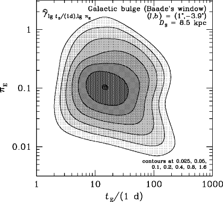
Figure 7: Bivariate distribution of the event rate with the time-scale $t_{\mathrm{E}}$ and the parallax parameter $\pi_{\mathrm{E}}=\pi_{\mathrm{LS}}/\theta_{\mathrm{E}}$. For a bulge source at $D_{\mathrm{S}}=8.5~{}\mathrm{kpc}$ in the direction of Baade’s window $(l,b)=(1\degr,-3.9\degr)$ and the Galaxy model described in Appendix B, contours of ${\hat{\gamma}}_{\lg[t_{\mathrm{E}}/(1d)],\lg\pi_{\mathrm{E}}}$ are shown at the levels $0.025$, $0.05$, $0.1$, $0.2$, $0.4$, $0.8$, and $1.6$.

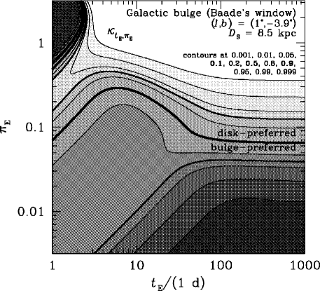
Figure 8: Fractional contribution $\kappa_{t_{\mathrm{E}},\pi_{\mathrm{E}}}^{\mathrm{disk}}$ of disk lenses and $\kappa_{t_{\mathrm{E}},\pi_{\mathrm{E}}}^{\mathrm{bulge}}$ of bulge lenses to the total event rate density $\gamma_{t_{\mathrm{E}},\pi_{\mathrm{E}}}$ as a function of the time-scale $t_{\mathrm{E}}$ and the parallax parameter $\pi_{\mathrm{E}}$ for a Galactic bulge source at $D_{\mathrm{S}}=8.5~{}\mathrm{kpc}$ towards Baade’s window. The set of contour levels at 0.001, 0.01, 0.05, 0.1, 0.2, 0.5, 0.8, 0.9, 0.95, 0.99, and 0.999 corresponds to both quantities, since $\kappa_{t_{\mathrm{E}},\pi_{\mathrm{E}}}^{\mathrm{disk}}+\kappa_{t_{\mathrm{E}},\pi_{\mathrm{E}}}^{\mathrm{bulge}}=1$. The contour at 0.5 is shown in bold, while the contours at 0.1 and 0.9 are shown in light bold.

Table 3: Fractional contributions $\kappa_{t_{\mathrm{E}},\pi_{\mathrm{E}}}^{\mathrm{disk}}$ and $\kappa_{t_{\mathrm{E}},\pi_{\mathrm{E}}}^{\mathrm{bulge}}$ of disk or bulge lenses to the event rate density $\gamma_{t_{\mathrm{E}},\pi_{\mathrm{E}}}(t_{\mathrm{E}},\pi_{\mathrm{E}})$ for a Galactic bulge source by lenses in the Galactic disk or bulge, respectively, for a typical $t_{\mathrm{E}}$ and selected $\pi_{\mathrm{E}}$.

$t_{\mathrm{E}}/(1~{}\mathrm{d})$	$\pi_{\mathrm{E}}$	$\kappa_{t_{\mathrm{E}},\pi_{\mathrm{E}}}^{\mathrm{disk}}$	$\kappa_{t_{\mathrm{E}},\pi_{\mathrm{E}}}^{\mathrm{bulge}}$
20	—	0.35	0.65
	0.015	0.05	0.95
	0.06	0.19	0.81
	0.25	0.80	0.20
	1	1.0	$3\times 10^{-6}$

With the event rate density ${\gamma}_{t_{\mathrm{E}},\pi_{\mathrm{E}}}$ given by Eq. (28), $\kappa_{t_{\mathrm{E}},\pi_{\mathrm{E}}}^{\mathrm{disk}}={\gamma}_{t_{\mathrm{E}},\pi_{\mathrm{E}}}^{\mathrm{disk}}/({\gamma}_{t_{\mathrm{E}},\pi_{\mathrm{E}}}^{\mathrm{disk}}+{\gamma}_{t_{\mathrm{E}},\pi_{\mathrm{E}}}^{\mathrm{bulge}})$ and $\kappa_{t_{\mathrm{E}},\pi_{\mathrm{E}}}^{\mathrm{bulge}}={\gamma}_{t_{\mathrm{E}},\pi_{\mathrm{E}}}^{\mathrm{bulge}}/({\gamma}_{t_{\mathrm{E}},\pi_{\mathrm{E}}}^{\mathrm{disk}}+{\gamma}_{t_{\mathrm{E}},\pi_{\mathrm{E}}}^{\mathrm{bulge}})$.

The measurement of the parallax parameter $\pi_{\mathrm{E}}^{(0)}$ in addition to the event time-scale $t_{\mathrm{E}}^{(0)}$ alters the fractional contributions of the individual lens populations to the event rate density for these values. The contributions of the Galactic disk given by $\kappa_{t_{\mathrm{E}},\pi_{\mathrm{E}}}^{\mathrm{disk}}={\gamma}_{t_{\mathrm{E}},\pi_{\mathrm{E}}}^{\mathrm{disk}}/({\gamma}_{t_{\mathrm{E}},\pi_{\mathrm{E}}}^{\mathrm{disk}}+{\gamma}_{t_{\mathrm{E}},\pi_{\mathrm{E}}}^{\mathrm{bulge}})$, while bulge lenses contribute the fraction $\kappa_{t_{\mathrm{E}},\pi_{\mathrm{E}}}^{\mathrm{bulge}}={\gamma}_{t_{\mathrm{E}},\pi_{\mathrm{E}}}^{\mathrm{bulge}}/({\gamma}_{t_{\mathrm{E}},\pi_{\mathrm{E}}}^{\mathrm{disk}}+{\gamma}_{t_{\mathrm{E}},\pi_{\mathrm{E}}}^{\mathrm{bulge}})$, are shown in Fig. 8. The corresponding values for the typical time-scale $t_{\mathrm{E}}^{(0)}=20~{}\mathrm{d}$ and a few different $\pi_{\mathrm{E}}^{(0)}$ are also listed in Table 3. Again, a bulge source at $D_{\mathrm{S}}=8.5~{}\mathrm{kpc}$ in the direction of Baade’s window has been assumed. By considering the contours at 0.1 and 0.9 together with the distribution of $t_{\mathrm{E}}$ and $\pi_{\mathrm{E}}$ as shown in Fig. 7, one sees that strong preferences for one of the populations are not unlikely to be provided, whereas Fig. 2 shows that from $t_{\mathrm{E}}$ the maximal preference for any time-scale is $\sim 0.8$ in favour of the bulge, achieved for $t_{\mathrm{E}}\sim 8~{}\mathrm{d}$. For $t_{\mathrm{E}}\ga 2.5~{}\mathrm{d}$, smaller values of $\pi_{\mathrm{E}}$ favour the lens to reside in the Galactic bulge, while larger $\pi_{\mathrm{E}}$ favour the disk as lens population. For smaller time-scales, there is an intermediate region where this order is reversed.

From the expression for the event rate density $\gamma_{\eta_{t_{\mathrm{E}}},\eta_{\pi_{\mathrm{E}}}}$ for an event with given $t_{\mathrm{E}}^{(0)}$ and $\pi_{\mathrm{E}}^{(0)}$, given by Eq. (27), one immediately finds the corresponding probability density of $\mu_{0}=M/M_{0}$ as

$$p_{\mu_{0}}^{(0)}(\mu_{0};\eta_{t_{\mathrm{E}}}^{(0)},\eta_{\pi_{\mathrm{E}}}^{(0)})=\frac{8\,\Gamma_{0}}{\gamma_{\eta_{t_{\mathrm{E}}},\eta_{\pi_{\mathrm{E}}}}(\eta_{t_{\mathrm{E}}}^{(0)},\eta_{\pi_{\mathrm{E}}}^{(0)})}\,[\eta_{t_{\mathrm{E}}}^{(0)}]^{5}\,[\eta_{\pi_{\mathrm{E}}}^{(0)}]^{4}\;\times$$

$$\times\;\frac{\mu_{0}^{3}}{\left\{1+\mu_{0}\,\left[\eta_{t_{\mathrm{E}}}^{(0)}\,\eta_{\pi_{\mathrm{E}}}^{(0)}\right]^{2}\right\}^{5}}\;\Phi_{M/M_{\sun}}\left(\mu_{0}\left[\eta_{t_{\mathrm{E}}}^{(0)}\right]^{2}\right)\;\times$$

$$\times\;\Phi_{\zeta}\left(\frac{2\,\mu_{0}\,\eta_{t_{\mathrm{E}}}^{(0)}\,\eta_{\pi_{\mathrm{E}}}^{(0)}}{1+\mu_{0}\,\left[\eta_{t_{\mathrm{E}}}^{(0)}\,\eta_{\pi_{\mathrm{E}}}^{(0)}\right]^{2}},\frac{1}{1+\mu_{0}\,\left[\eta_{t_{\mathrm{E}}}^{(0)}\,\eta_{\pi_{\mathrm{E}}}^{(0)}\right]^{2}}\right)\;\times$$

$$\times\;\Phi_{x}\left(\frac{1}{1+\mu_{0}\,\left[\eta_{t_{\mathrm{E}}}^{(0)}\,\eta_{\pi_{\mathrm{E}}}^{(0)}\right]^{2}}\right)\,.$$ (29)

The probability density of the fractional lens distance $x$ for observed $t_{\mathrm{E}}^{(0)}$ and $\pi_{\mathrm{E}}^{(0)}$ can be obtained with Eq. (15) by applying the parallax constraint in the form $\delta[\eta_{\pi_{\mathrm{E}}}^{(0)}-\sqrt{(1-x)/(\mu_{0}\,x)}/\eta_{t_{\mathrm{E}}}^{(0)}]$, yielding

$$p_{x}^{(0)}(x;\eta_{t_{\mathrm{E}}}^{(0)},\eta_{\pi_{\mathrm{E}}}^{(0)})=\frac{8\,\Gamma_{0}}{\gamma_{\eta_{t_{\mathrm{E}}},\eta_{\pi_{\mathrm{E}}}}(\eta_{t_{\mathrm{E}}}^{(0)},\eta_{\pi_{\mathrm{E}}}^{(0)})}\,\frac{1}{[\eta_{t_{\mathrm{E}}}^{(0)}]^{3}\,[\eta_{\pi_{\mathrm{E}}}^{(0)}]^{4}}\;\times$$

$$\times\;(1-x)^{3}\;\Phi_{M/M_{\sun}}\left(\left[\eta_{\pi_{\mathrm{E}}}^{(0)}\right]^{-2}\,\frac{1-x}{x}\right)\;\times$$

$$\times\;\Phi_{\zeta}\left(\frac{2\,(1-x)}{\eta_{t_{\mathrm{E}}}^{(0)}\eta_{\pi_{\mathrm{E}}}^{(0)}},x\right)\,\Phi_{x}(x)\,.$$ (30)

For deriving $p_{\zeta}^{(0)}(\zeta;\eta_{t_{\mathrm{E}}}^{(0)},\eta_{\pi_{\mathrm{E}}}^{(0)})$, one can first eliminate $x$ with the time-scale constraint in Eq. (86) in order to obtain Eq. (17) and then use the parallax constraint in the form $\delta[\eta_{\pi_{\mathrm{E}}}^{(0)}-(1\mp\sqrt{1-\zeta^{2}/\mu_{0}})/(\eta_{t_{\mathrm{E}}}^{(0)}\,\zeta)]$, or alternatively first eliminate $\mu_{0}$ and then use $\delta[\eta_{\pi_{\mathrm{E}}}^{(0)}-2\,(1-x)/(\zeta\,\eta_{t_{\mathrm{E}}}^{(0)})]$ as parallax constraint. Regardless of the way of approach, one obtains

$$p_{\zeta}^{(0)}(\zeta;\eta_{t_{\mathrm{E}}}^{(0)},\eta_{\pi_{\mathrm{E}}}^{(0)})=\frac{\Gamma_{0}}{2\,\gamma_{\eta_{t_{\mathrm{E}}},\eta_{\pi_{\mathrm{E}}}}(\eta_{t_{\mathrm{E}}}^{(0)},\eta_{\pi_{\mathrm{E}}}^{(0)})}\,\eta_{t_{\mathrm{E}}}^{(0)}\;\times$$

$$\times\;\zeta^{3}\;\Theta\left(1-\frac{\zeta\,\eta_{t_{\mathrm{E}}}^{(0)}\eta_{\pi_{\mathrm{E}}}^{(0)}}{2}\right)\;\times$$

$$\times\;\Phi_{M/M_{\sun}}\left(\frac{\zeta\,\eta_{t_{\mathrm{E}}}^{(0)}}{\eta_{\pi_{\mathrm{E}}}^{(0)}\,\left(2-\zeta\,\eta_{t_{\mathrm{E}}}^{(0)}\eta_{\pi_{\mathrm{E}}}^{(0)}\right)}\right)\;\times$$

$$\times\;\Phi_{\zeta}\left(\zeta,1-\frac{\zeta\,\eta_{t_{\mathrm{E}}}^{(0)}\eta_{\pi_{\mathrm{E}}}^{(0)}}{2}\right)\,\Phi_{x}\left(1-\frac{\zeta\,\eta_{t_{\mathrm{E}}}^{(0)}\eta_{\pi_{\mathrm{E}}}^{(0)}}{2}\right)\,.$$ (31)

Figure 9: Probability densities of $\lg(M/M_{\sun})$, the fractional lens distance $x$ and $\lg\zeta$, where $\zeta=v/v_{\mathrm{c}}$ and $v_{\mathrm{c}}=100~{}\mathrm{km}\,\mathrm{s}^{-1}$, for $t_{\mathrm{E}}=20~{}\mathrm{d}$ and $\pi_{\mathrm{E}}=0.015,0.06,0.25,\mathrm{or}~{}1.0$ (solid lines) as well as that for an uncertain $\pi_{\mathrm{E}}$, i.e. based solely on the time-scale $t_{\mathrm{E}}$ (dotted line). The source is thereby located in the Galactic bulge at $D_{\mathrm{S}}=8.5~{}\mathrm{kpc}$ in the direction of Baade’s window $(l,b)=(1\degr,-3.9\degr)$.

Table 4: Expectation value and standard deviation for the lens properties $\lg(M/M_{\sun})$, $x$, and $\lg\zeta$ for an event with time-scale $t_{\mathrm{E}}$ and parallax parameter $\pi_{\mathrm{E}}$.

$t_{\mathrm{E}}/(1~{}\mathrm{d})$	$\pi_{\mathrm{E}}$	$\left\langle\lg(M/M_{\sun})\right\rangle$	$\sigma_{\lg(M/M_{\sun})}$	${\hat{M}}/M_{\sun}$	$\varsigma_{M/{\hat{M}}}$	$\left\langle x\right\rangle$	$\sigma_{x}$	$\left\langle\lg\zeta\right\rangle$	$\sigma_{\lg\zeta}$	${\hat{v}}/(100~{}\mathrm{km}\,\mathrm{s}^{-1})$	$\varsigma_{v/{\hat{v}}}$
20	—	-0.45	0.39	0.36	2.5	0.77	0.15	0.21	0.17	161	1.5
	0.015	0.41	0.20	2.55	1.6	0.96	0.02	0.34	0.20	219	1.6
	0.06	-0.21	0.18	0.62	1.5	0.86	0.05	0.28	0.16	190	1.4
	0.25	-0.85	0.18	0.14	1.5	0.62	0.09	0.11	0.12	129	1.3
	1	-1.29	0.34	0.05	2.2	0.25	0.01	-0.19	0.08	64	1.2

The row with $\pi_{\mathrm{E}}$ marked ’—’ corresponds to an uncertain parallax parameter, i.e. the estimate is based solely on $t_{\mathrm{E}}$. Also listed are the exponentiated values ${\hat{M}}/M_{\sun}=\exp_{10}[\left\langle\lg(M/M_{\sun})\right\rangle]$ and $\varsigma_{M/{\hat{M}}}=\exp_{10}[\sigma_{\lg(M/M_{\sun})}]$ as well as ${\hat{v}}=\exp_{10}[\left\langle\lg\zeta\right\rangle]\,v_{\mathrm{c}}$ and $\varsigma_{v/{\hat{v}}}=\exp_{10}[\sigma_{\lg\zeta}]$. The source is located in the Galactic bulge at $D_{\mathrm{S}}=8.5~{}\mathrm{kpc}$ in the direction of Baade’s window $(l,b)=(1\degr,-3.9\degr)$, and the Galaxy model described in Appendix B has been adopted.

For a typical time-scale $t_{\mathrm{E}}^{(0)}=20~{}\mathrm{d}$ and different values for the parallax parameter $\pi_{\mathrm{E}}^{(0)}$, the probability densities $p_{\lg(M/M_{\sun})}$, $p_{x}$, and $p_{\lg\zeta}$ are shown in Fig. 9, whereas expectation values and standard deviations for the related quantities are listed in Table 4. For comparison, the previously obtained results for an uncertain $\pi_{\mathrm{E}}$, i.e. based solely on the measured time-scale $t_{\mathrm{E}}^{(0)}$ are also shown. In most cases, the measurement of the parallax parameter results in a significant reduction of the width of the distribution, equivalent to a reduction of the uncertainty of the considered lens property, where the mass estimate improves most significantly. If, however, the parallax constraint forces the lens properties to fall into an a-priori disfavoured region, the expectation value is strongly shifted and the distribution may widen. The uncertainty is still dominated by the mass spectrum, mass density and velocity distributions as compared to the contribution arising from the finite width of the time-scale distribution. As a result of the finite limits on the lens mass from the spectrum $\Phi_{M/M_{\sun}}$ and the condition $0\leq x\leq 1$, the probability densities of the lens properties may face sudden cut-offs.

5.3 Finite source size

For a finite-source event with observed $t_{\mathrm{E}}^{(0)}$ and $t_{\star}^{(0)}$ and the related $\eta_{t_{\mathrm{E}}}^{(0)}$ and $\eta_{t_{\star}}^{(0)}$ as given by Eqs. (11) and (26), the event rate density $\gamma_{\eta_{t_{\mathrm{E}}},\eta_{t_{\star}}}(\eta_{t_{\mathrm{E}}}^{(0)},\eta_{t_{\star}}^{(0)})$ results from Eq. (12) by applying the additional constraint $\delta[\eta_{t_{\star}}^{(0)}-\sqrt{x/(1-x)}\,(M/M_{\sun})^{-1/2}]$. If one compares this with the case of parallax effects, one finds that $\eta_{\pi_{\mathrm{E}}}^{(0)}$ assumes the role of $\eta_{t_{\star}}^{(0)}$ while $x$ and $1-x$ are interchanged, which is reflected in the result

$$\gamma_{\eta_{t_{\mathrm{E}}},\eta_{t_{\star}}}(\eta_{t_{\mathrm{E}}}^{(0)},\eta_{t_{\star}}^{(0)})=8\,\Gamma_{0}\,\frac{[\eta_{t_{\star}}^{(0)}]^{4}}{[\eta_{t_{\mathrm{E}}}^{(0)}]^{3}}\;\times$$

$$\times\;\int\limits_{M_{\mathrm{min}}/M_{\sun}}^{M_{\mathrm{max}}/M_{\sun}}\frac{(M/M_{\sun})^{3}}{\left\{1+[\eta_{t_{\star}}^{(0)}]^{2}\,(M/M_{\sun})\right\}^{5}}\;\times$$

$$\times\;\Phi_{M/M_{\sun}}\left(\mu_{0}\left[\eta_{t_{\mathrm{E}}}^{(0)}\right]^{2}\right)\;\times$$

$$\times\;\Phi_{\zeta}\left(\frac{2\,(\eta_{t_{\star}}^{(0)}/\eta_{t_{\mathrm{E}}}^{(0)})\,(M/M_{\sun})}{1+[\eta_{t_{\star}}^{(0)}]^{2}\,(M/M_{\sun})},\frac{[\eta_{t_{\star}}^{(0)}]^{2}\,(M/M_{\sun})}{1+[\eta_{t_{\star}}^{(0)}]^{2}\,(M/M_{\sun})}\right)\;\times$$

$$\times\;\Phi_{x}\left(\frac{[\eta_{t_{\star}}^{(0)}]^{2}\,(M/M_{\sun})}{1+[\eta_{t_{\star}}^{(0)}]^{2}\,(M/M_{\sun})}\right)\,\mathrm{d}(M/M_{\sun})\,.$$ (32)

The event rate density in $(t_{\mathrm{E}},t_{\star})$ follows directly as

$$\gamma_{t_{\mathrm{E}},t_{\star}}(t_{\mathrm{E}}^{(0)},t_{\star}^{(0)})$$

$$=\frac{2\,v_{\mathrm{c}}}{R_{\star}\,t_{\mathrm{E}}^{(0)}}\;\gamma_{\eta_{t_{\mathrm{E}}},\eta_{\pi_{\mathrm{E}}}}\left(\frac{v_{\mathrm{c}}}{r_{\mathrm{E},\sun}}\,t_{\mathrm{E}}^{(0)},2\,\frac{r_{\mathrm{E},\sun}}{R_{\star}}\,\frac{t_{\star}^{(0)}}{t_{\mathrm{E}}^{(0)}}\right)\,,$$ (33)

so that with ${\hat{\rho}}_{\star,\sun}=(t_{\star}/t_{\mathrm{E}})\,(R_{\star}/R_{\sun})^{-1}$, one finds $(t_{\mathrm{E}},{\hat{\rho}}_{\star,\sun})$ to follow the distribution

$${\hat{\gamma}}_{t_{\mathrm{E}},{\hat{\rho}}_{\star,\sun}}(t_{\mathrm{E}}^{(0)},{\hat{\rho}}_{\star,\sun}^{(0)})$$

$$=\frac{2}{\Gamma}\,\frac{v_{\mathrm{c}}}{R_{\star}}\;\gamma_{\eta_{t_{\mathrm{E}}},\eta_{\pi_{\mathrm{E}}}}\left(\frac{v_{\mathrm{c}}}{r_{\mathrm{E},\sun}}\,t_{\mathrm{E}}^{(0)},2\,\frac{r_{\mathrm{E}},\sun}{R_{\star}}\,{\hat{\rho}}_{\star,\sun}^{(0)}\right)\,.$$ (34)

Fig. 11 shows the fractional contribution $\kappa_{t_{\mathrm{E}},t_{\star}}$ to the event rate density for a given $t_{\mathrm{E}}$ and $t_{\star}$ for the lens residing in either the Galactic bulge or disk. The measurement of finite-source effects turns out to be less powerful than that of parallax with most of the likely values not providing strong preference for either of the lens populations. However, small $t_{\star}/t_{\mathrm{E}}$ Bulge lenses are preferred for intermediate values $0.0015\la(t_{\star}/t_{\mathrm{E}})(R_{\star}/R_{\sun})^{-1}\la 0.007$, where a strong preference however can only arise for $t_{\mathrm{E}}\la 10~{}\mathrm{d}$. Measurements of a small $t_{\star}/t_{\mathrm{E}}$ can provide a very strong preference for the lens to reside in the disk.

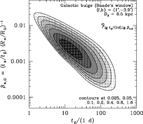
Figure 10: Bivariate distribution of the event rate with the time-scale $t_{\mathrm{E}}$ and the finite-source parameter ${\hat{\rho}}_{\star,\sun}=(t_{\star}/t_{\mathrm{E}})\,(R_{\star}/R_{\sun})^{-1}$. The source is located in the Galactic bulge at $D_{\mathrm{S}}=8.5~{}\mathrm{kpc}$ in the direction of Baade’s window $(l,b)=(1\degr,-3.9\degr)$. The plot shows contours of ${\hat{\gamma}}_{\lg[t_{\mathrm{E}}/(1d)],\lg\pi_{\mathrm{E}}}$ correspond to the levels $0.025$, $0.05$, $0.1$, $0.2$, $0.4$, $0.8$, and $1.6$.

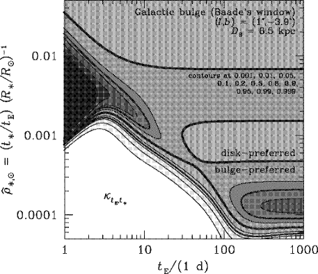
Figure 11: Fractional contribution $\kappa_{t_{\mathrm{E}},t_{\star}}^{\mathrm{disk}}$ of disk lenses and $\kappa_{t_{\mathrm{E}},\star}^{\mathrm{bulge}}$ of bulge lenses to the total event rate density $\gamma_{t_{\mathrm{E}},t_{\star}}$ as a function of the time-scale $t_{\mathrm{E}}$ and the finite-source time-scale $t_{\star}=t_{\mathrm{E}}\,[R_{\star}/(D_{\mathrm{S}}\,\theta_{\mathrm{E}})]$ for a Galactic bulge source at $D_{\mathrm{S}}=8.5~{}\mathrm{kpc}$ towards Baade’s window. With $\kappa_{t_{\mathrm{E}},\pi_{\mathrm{E}}}^{\mathrm{disk}}+\kappa_{t_{\mathrm{E}},\pi_{\mathrm{E}}}^{\mathrm{bulge}}=1$, the set of contour levels at 0.001, 0.01, 0.05, 0.1, 0.2, 0.5, 0.8, 0.9, 0.95, 0.99, and 0.999 corresponds to both quantities. The contour at the level 0.5 is shown in bold, while light bold has been used for the contours at 0.1 and 0.9.

Table 5: Fractional contributions $\kappa_{t_{\mathrm{E}},t_{\star}}^{\mathrm{disk}}$ and $\kappa_{t_{\mathrm{E}},t_{\star}}^{\mathrm{bulge}}$ of disk or bulge lenses to the event rate density $\gamma_{t_{\mathrm{E}},t_{\star}}(t_{\mathrm{E}},t_{\star})$ for a Galactic bulge source by lenses in the Galactic disk or bulge, respectively, for a typical $t_{\mathrm{E}}$ and selected ${\hat{\rho}}_{\star,\sun}=(t_{\star}/t_{\mathrm{E}})\,(R_{\star}/R_{\sun})^{-1}$.

$t_{\mathrm{E}}/(1~{}\mathrm{d})$	${\hat{\rho}}_{\star,\sun}$	$\kappa_{t_{\mathrm{E}},t_{\star}}^{\mathrm{disk}}$	$\kappa_{t_{\mathrm{E}},t_{\star}}^{\mathrm{bulge}}$
20	—	0.35	0.65
	0.0005	0.83	0.17
	0.00125	0.35	0.65
	0.003	0.34	0.66
	0.0075	0.52	0.48

With the event rate density ${\gamma}_{t_{\mathrm{E}},t_{\star}}$ given by Eq. (33), $\kappa_{t_{\mathrm{E}},t_{\star}}^{\mathrm{disk}}={\gamma}_{t_{\mathrm{E}},t_{\star}}^{\mathrm{disk}}/({\gamma}_{t_{\mathrm{E}},t_{\star}}^{\mathrm{disk}}+{\gamma}_{t_{\mathrm{E}},t_{\star}}^{\mathrm{bulge}})$ and $\kappa_{t_{\mathrm{E}},t_{\star}}^{\mathrm{bulge}}={\gamma}_{t_{\mathrm{E}},t_{\star}}^{\mathrm{bulge}}/({\gamma}_{t_{\mathrm{E}},t_{\star}}^{\mathrm{disk}}+{\gamma}_{t_{\mathrm{E}},t_{\star}}^{\mathrm{bulge}})$.

From Eq. (32), the probability density of $\mu_{0}$ follows as

$$p_{\mu_{0}}^{(0)}(\mu_{0};\eta_{t_{\mathrm{E}}}^{(0)},\eta_{t_{\star}}^{(0)})=\frac{8\,\Gamma_{0}}{\gamma_{\eta_{t_{\mathrm{E}}},\eta_{t_{\star}}}(\eta_{t_{\mathrm{E}}}^{(0)},\eta_{t_{\star}}^{(0)})}\,[\eta_{t_{\mathrm{E}}}^{(0)}]^{5}\,[\eta_{t_{\star}}^{(0)}]^{4}\;\times$$

$$\times\;\frac{\mu_{0}^{3}}{\left\{1+\mu_{0}\,\left[\eta_{t_{\mathrm{E}}}^{(0)}\,\eta_{t_{\star}}^{(0)}\right]^{2}\right\}^{5}}\;\Phi_{M/M_{\sun}}\left(\mu_{0}\left[\eta_{t_{\mathrm{E}}}^{(0)}\right]^{2}\right)\;\times$$

$$\times\;\Phi_{\zeta}\left(\frac{2\,\mu_{0}\,\eta_{t_{\mathrm{E}}}^{(0)}\,\eta_{t_{\star}}^{(0)}}{1+\mu_{0}\,\left[\eta_{t_{\mathrm{E}}}^{(0)}\,\eta_{t_{\star}}^{(0)}\right]^{2}},\frac{\mu_{0}\,\left[\eta_{t_{\mathrm{E}}}^{(0)}\,\eta_{t_{\star}}^{(0)}\right]^{2}}{1+\mu_{0}\,\left[\eta_{t_{\mathrm{E}}}^{(0)}\,\eta_{t_{\star}}^{(0)}\right]^{2}}\right)\;\times$$

$$\times\;\Phi_{x}\left(\frac{\mu_{0}\,\left[\eta_{t_{\mathrm{E}}}^{(0)}\,\eta_{t_{\star}}^{(0)}\right]^{2}}{1+\mu_{0}\,\left[\eta_{t_{\mathrm{E}}}^{(0)}\,\eta_{t_{\star}}^{(0)}\right]^{2}}\right)\,,$$ (35)

while for the probability density of $x$, one finds

$$p_{x}^{(0)}(x;\eta_{t_{\mathrm{E}}}^{(0)},\eta_{t_{\star}}^{(0)})=\frac{8\,\Gamma_{0}}{\gamma_{\eta_{t_{\mathrm{E}}},\eta_{t_{\star}}}(\eta_{t_{\mathrm{E}}}^{(0)},\eta_{t_{\star}}^{(0)})}\,\frac{1}{[\eta_{t_{\mathrm{E}}}^{(0)}]^{3}\,[\eta_{t_{\star}}^{(0)}]^{4}}\;\times$$

$$\times\;x^{3}\;\Phi_{M/M_{\sun}}\left(\left[\eta_{t_{\star}}^{(0)}\right]^{-2}\,\frac{x}{1-x}\right)\;\times$$

$$\times\;\Phi_{\zeta}\left(\frac{2\,x}{\eta_{t_{\mathrm{E}}}^{(0)}\eta_{t_{\star}}^{(0)}},x\right)\,\Phi_{x}(x)\,.$$ (36)

After elimination of $\mu_{0}$ using the constraint provided by $t_{\mathrm{E}}^{(0)}$, the finite-source constraint becomes $\delta[\eta_{t_{\star}}^{(0)}-2\,x/(\zeta\,\eta_{t_{\mathrm{E}}}^{(0)})]$, while the elimination of $x$ yields the constraint $\delta[\eta_{t_{\star}}^{(0)}-(1\pm\sqrt{1-\zeta^{2}/\mu_{0}})/(\eta_{t_{\mathrm{E}}}^{(0)}\,\zeta)]$, so that either with Eq. (17) or directly from Eq. (86), one obtains the probability density of $\zeta$ for measured $t_{\mathrm{E}}^{(0)}$ and $t_{\star}^{(0)}$ as

$$p_{\zeta}^{(0)}(\zeta;\eta_{t_{\mathrm{E}}}^{(0)},\eta_{t_{\star}}^{(0)})=\frac{\Gamma_{0}}{2\,\gamma_{\eta_{t_{\mathrm{E}}},\eta_{t_{\star}}}(\eta_{t_{\mathrm{E}}}^{(0)},\eta_{t_{\star}}^{(0)})}\,\eta_{t_{\mathrm{E}}}^{(0)}\;\times$$

$$\times\;\zeta^{3}\;\Theta\left(\frac{\zeta\,\eta_{t_{\mathrm{E}}}^{(0)}\eta_{t_{\star}}^{(0)}}{2}\right)\times\;$$

$$\times\;\Phi_{M/M_{\sun}}\left(\frac{\zeta\,\eta_{t_{\mathrm{E}}}^{(0)}}{\eta_{t_{\star}}^{(0)}\,\left(2-\zeta\,\eta_{t_{\mathrm{E}}}^{(0)}\eta_{t_{\star}}^{(0)}\right)}\right)\;\times$$

$$\times\;\Phi_{\zeta}\left(\zeta,\frac{\zeta\,\eta_{t_{\mathrm{E}}}^{(0)}\eta_{t_{\star}}^{(0)}}{2}\right)\,\Phi_{x}\left(\frac{\zeta\,\eta_{t_{\mathrm{E}}}^{(0)}\eta_{t_{\star}}^{(0)}}{2}\right)\,.$$ (37)

Figure 12: Probability densities of $\lg(M/M_{\sun})$, the fractional lens distance $x$ and $\lg\zeta$, where $\zeta=v/v_{\mathrm{c}}$ and $v_{\mathrm{c}}=100~{}\mathrm{km}\,\mathrm{s}^{-1}$, for $t_{\mathrm{E}}=20~{}\mathrm{d}$ and ${\hat{\rho}}_{\star,\sun}=(t_{\star}/t_{\mathrm{E}})\,(R_{\star}/R_{\sun})^{-1}=0.0005,0.00125,0.003,\mathrm{or}~{}0.0075$ (solid lines) as well as that for an uncertain $t_{\star}$, i.e. based solely on the time-scale $t_{\mathrm{E}}$ (dotted line). The source is located in the Galactic bulge at $D_{\mathrm{S}}=8.5~{}\mathrm{kpc}$ in the direction of Baade’s window $(l,b)=(1\degr,-3.9\degr)$.

Table 6: Expectation value and standard deviation for the lens properties $\lg(M/M_{\sun})$, $x$, and $\lg\zeta$ for an event with time-scale $t_{\mathrm{E}}$ and finite-source parameter ${\hat{\rho}}_{\star,\sun}=(t_{\star}/t_{\mathrm{E}})\,(R_{\star}/R_{\sun})^{-1}$.

$t_{\mathrm{E}}/(1~{}\mathrm{d})$	${\hat{\rho}}_{\star,\sun}$	$\left\langle\lg(M/M_{\sun})\right\rangle$	$\sigma_{\lg(M/M_{\sun})}$	${\hat{M}}/M_{\sun}$	$\varsigma_{M/{\hat{M}}}$	$\left\langle x\right\rangle$	$\sigma_{x}$	$\left\langle\lg\zeta\right\rangle$	$\sigma_{\lg\zeta}$	${\hat{v}}/(100~{}\mathrm{km}\,\mathrm{s}^{-1})$	$\varsigma_{v/{\hat{v}}}$
20	—	-0.45	0.39	0.36	2.5	0.77	0.15	0.21	0.17	161	1.5
	0.0005	-0.71	0.46	0.19	2.9	0.18	0.18	0.00	0.33	99	2.2
	0.00125	-0.26	0.36	0.56	2.3	0.71	0.16	0.35	0.12	222	1.3
	0.003	-0.67	0.33	0.22	2.1	0.84	0.11	0.04	0.07	111	1.2
	0.0075	-1.05	0.43	0.09	2.7	0.92	0.08	-0.31	0.04	49	1.1

For the row with the entry ’—’ for ${\hat{\rho}}_{\star,\sun}$, the estimate is based solely on $t_{\mathrm{E}}$, while the finite-source parameter has been considered as uncertain. In addition to the basic estimates, the exponentiated values ${\hat{M}}/M_{\sun}=\exp_{10}[\left\langle\lg(M/M_{\sun})\right\rangle]$ and $\varsigma_{M/{\hat{M}}}=\exp_{10}[\sigma_{\lg(M/M_{\sun})}]$ as well as ${\hat{v}}=\exp_{10}[\left\langle\lg\zeta\right\rangle]\,v_{\mathrm{c}}$ and $\varsigma_{v/{\hat{v}}}=\exp_{10}[\sigma_{\lg\zeta}]$ are listed. The source is located in the Galactic bulge at $D_{\mathrm{S}}=8.5~{}\mathrm{kpc}$ in the direction of Baade’s window $(l,b)=(1\degr,-3.9\degr)$, and the Galaxy model described in Appendix B has been adopted.

Fig. 12 shows the probability densities of $\lg(M/M_{\sun})$, the fractional lens distance $x$, and $\lg\zeta$ for a microlensing event on a bulge source at $D_{\mathrm{S}}=8.5~{}\mathrm{kpc}$ in the direction of Baade’s window for which $t_{\mathrm{E}}$ and $t_{\star}$ have been determined, where a typical time-scale $t_{\mathrm{E}}^{(0)}=20~{}\mathrm{d}$ has been assumed, whereas a few different values for ${\hat{\rho}}_{\star,\sun}^{(0)}$ have been chosen. For the same values, Table 5 shows the fractional contributions of the bulge and disk lenses to the event rate density $\gamma_{t_{\mathrm{E}},t_{\star}}(t_{\mathrm{E}}^{(0)},t_{\star}^{(0)})$. While the parallax measurement has been found to provide the most effective reduction of uncertainty for the lens mass, one finds that the finite-source parameter ${\hat{\rho}}_{\star,\sun}$ or the related time-scale $t_{\star}$ most significantly affects the uncertainty in the effective transverse velocity $v=v_{\mathrm{c}}\,\zeta$ or the related Einstein radius $r_{\mathrm{E}}=t_{\mathrm{E}}\,v$. Some distributions show two peaks corresponding to the bulge and disk population.

5.4 Combination of parallax and finite-source effects

If both $\pi_{\mathrm{E}}$ and $t_{\star}$ are measured, the lens mass $M$, its fractional distance $x$, and the effective velocity $v$ are determined, so that

$$p_{\mu_{0}}^{(0)}(\mu_{0};\eta_{t_{\mathrm{E}}}^{(0)},\eta_{\pi_{\mathrm{E}}}^{(0)},\eta_{t_{\star}}^{(0)})=\delta\left(\mu_{0}-\frac{1}{\left[\eta_{t_{\mathrm{E}}}^{(0)}\right]^{2}\,\eta_{\pi_{\mathrm{E}}}^{(0)}\,\eta_{t_{\star}}^{(0)}}\right)\,,$$ (38)

and the uncertainty in these quantities is solely given by the distributions of the model parameters $t_{\mathrm{E}}$, $\pi_{\mathrm{E}}$, and $t_{\star}$ or the related dimensionless $\eta_{t_{\mathrm{E}}}$, $\eta_{\pi_{\mathrm{E}}}$, and $\eta_{t_{\star}}$, respectively.

As result of a fundamental property of logarithms and the linearity of the expectation value, the expectation value of the logarithm of a product of arbitrary powers of quantities $\xi_{i}$ separates into the sum of multiples of the expectation values of the logarithms of the individual quantities, i.e.

$$\left\langle\lg\prod\limits_{i=1}^{k}\xi_{i}^{\beta_{i}}\right\rangle=\left\langle\sum\limits_{i=1}^{k}\beta_{i}\,\lg\xi_{i}\right\rangle=\sum\limits_{i=1}^{k}\beta_{i}\,\left\langle\lg\xi_{i}\right\rangle\,.$$ (39)

Similarly, one finds for the variances

$$\mathrm{Var}\left(\lg\prod\limits_{i=1}^{k}\xi_{i}^{\beta_{i}}\right)=\sum\limits_{i=1}^{k}\sum\limits_{j=1}^{k}\beta_{i}\beta_{j}\,\mathrm{Cov}\left(\lg\xi_{i},\lg\xi_{j}\right)\,,$$ (40)

where $\mathrm{Cov}(x_{i},x_{j})=\mathrm{Cov}(x_{j},x_{i})$ denotes the covariance of the quantities $x_{i}$ and $x_{j}$, and $\mathrm{Cov}(x_{i},x_{i})=\mathrm{Var}(x_{i})$.

While one naively finds the lens mass as

$$M=\frac{c^{2}}{4G}\,\frac{1~{}\mathrm{AU}}{\pi_{\mathrm{E}}}\,\frac{t_{\mathrm{E}}}{t_{\star}}\,\theta_{\star}\,,$$ (41)

taking into account the finite uncertainties yields

$$\left\langle\lg\frac{M}{M_{\sun}}\right\rangle=\lg\left[\frac{c^{2}}{4GM_{\sun}}\,(1~{}\mathrm{AU})\right]+\left\langle\lg\frac{t_{\mathrm{E}}}{1~{}\mathrm{d}}\right\rangle-\left\langle\lg\frac{t_{\star}}{1~{}\mathrm{d}}\right\rangle\;-$$

$$-\;\left\langle\lg\pi_{\mathrm{E}}\right\rangle+\left\langle\lg\theta_{\star}\right\rangle\,,$$ (42)

and with $\theta_{\star}=R_{\star}/D_{\mathrm{S}}$ not being correlated with the model parameters $t_{\mathrm{E}}$, $t_{\star}$, and $\pi_{\mathrm{E}}$, one obtains

$$\mathrm{Var}\left(\lg\frac{M}{M_{\sun}}\right)=\mathrm{Var}\left(\lg\frac{t_{\mathrm{E}}}{1~{}\mathrm{d}}\right)+\mathrm{Var}\left(\lg\frac{t_{\star}}{1~{}\mathrm{d}}\right)\;+$$

$$+\;\mathrm{Var}\left(\lg\pi_{\mathrm{E}}\right)+\mathrm{Var}\left(\lg\frac{R_{\star}}{1~{}\mathrm{d}}\right)+\mathrm{Cov}\left(\lg\frac{t_{\mathrm{E}}}{1~{}\mathrm{d}},\lg\frac{t_{\star}}{1~{}\mathrm{d}}\right)\;+$$

$$+\;\mathrm{Cov}\left(\lg\frac{t_{\mathrm{E}}}{1~{}\mathrm{d}},\lg\pi_{\mathrm{E}}\right)+\mathrm{Cov}\left(\lg\frac{t_{\star}}{1~{}\mathrm{d}},\lg\pi_{\mathrm{E}}\right)\,.$$ (43)

5.5 Limits arising from the absence of anomalous effects

Table 7: Constraint on the fractional lens distance $x\equiv D_{\mathrm{L}}/D_{\mathrm{S}}$ arising from upper limits on the annual parallax or the source size.

		${\tilde{x}}^{\mathrm{min}}$
$\pi_{\mathrm{E}}$	$\eta_{\pi_{\mathrm{E}}}$	0.1 $M_{\sun}$	0.2 $M_{\sun}$	0.4 $M_{\sun}$	0.8 $M_{\sun}$
0.015	0.12	0.998	0.997	0.994	0.988
0.06	0.50	0.98	0.95	0.91	0.83
0.25	2.1	0.70	0.54	0.37	0.22
1	8.3	0.13	0.07	0.03	0.02

		${\tilde{x}}^{\mathrm{max}}$
${\hat{\rho}}_{\star,\sun}$	$\eta_{t_{\star}}$	0.1 $M_{\sun}$	0.2 $M_{\sun}$	0.4 $M_{\sun}$	0.8 $M_{\sun}$
0.0005	0.89	0.07	0.14	0.24	0.39
0.00125	2.2	0.33	0.50	0.67	0.80
0.003	5.4	0.74	0.85	0.92	0.96
0.0075	13	0.95	0.97	0.986	0.993

The source star has been assumed to be located at a distance $D_{\mathrm{S}}=8.5~{}\mathrm{kpc}$ in the direction of Baade’s window. $\eta_{\pi_{\mathrm{E}}}=2[r_{\mathrm{E},\sun}/(1~{}\mathrm{AU})]\pi_{\mathrm{E}}$, $\eta_{t_{\star}}=2(r_{\mathrm{E},\sun}/R_{\sun}){\hat{\rho}}_{\star,\sun}$.

Frequently, anomalous effects such as those caused by the annual parallax or the finite source size escape detection from the photometric data taken over the course of the microlensing event. However, the absence of significant deviations from a lightcurve that is compatible with an ordinary event places upper limits on the model parameters $\pi_{\mathrm{E}}$ or $t_{\star}$. Rather than ”defining” a certain value by means of $\delta$-functions, these constraints can be incorporated by including $\Theta$-functions in the respective expressions for the probability and event rate densities. With $\eta_{\pi_{\mathrm{E}}}=[(1-x)/x]^{1/2}\,(M/M_{\sun})^{-1/2}$ and $\eta_{\pi_{\mathrm{E}}}\leq\eta_{\pi_{\mathrm{E}}}^{\mathrm{max}}$, one finds a lower limit on the fractional lens distance

$$x\geq{\tilde{x}}^{\mathrm{min}}=\frac{1}{1+\left(\eta_{\pi_{\mathrm{E}}}^{\mathrm{max}}\right)^{2}\,(M/M_{\sun})}$$ (44)

for a given mass $M$. In analogy, for the finite source size, one finds with $\eta_{t_{\star}}=[x/(1-x)]^{1/2}\,(M/M_{\sun})^{-1/2}$ and $\eta_{t_{\star}}\leq\eta_{t_{\star}}^{\mathrm{max}}$ an upper limit

$$x\leq{\tilde{x}}^{\mathrm{max}}=\frac{\left(\eta_{t_{\star}}^{\mathrm{max}}\right)^{2}\,(M/M_{\sun})}{1+\left(\eta_{t_{\star}}^{\mathrm{max}}\right)^{2}\,(M/M_{\sun})}\,.$$ (45)

Taking into account these limits yields e.g. the probability density of the lens mass $\mu_{0}=M/M_{0}$ in generalization of Eq. (13) as

$$p_{\mu_{0}}^{(0)}(\mu_{0};\eta_{t_{\mathrm{E}}}^{(0)})=\frac{4\,\Gamma_{0}}{\gamma_{\eta_{t_{\mathrm{E}}}}(\eta_{t_{\mathrm{E}}}^{(0)})}\,\sqrt{\mu_{0}}\;\Phi_{M/M_{\sun}}\left(\mu_{0}\left[\eta_{t_{\mathrm{E}}}^{(0)}\right]^{2}\right)\;\times$$

$$\times\;\int\limits_{{\tilde{x}}^{\mathrm{min}}(\mu_{0})}^{{\tilde{x}}^{\mathrm{max}}(\mu_{0})}\Phi_{\zeta}\left(2\,\sqrt{\mu_{0}\,x(1-x)},x\right)\;\times$$

$$\times\;[x(1-x)]^{3/2}\,\Phi_{x}(x)\,\mathrm{d}x\,.$$ (46)

Figure 13: Probability densities of $\lg(M/M_{\sun})$ for an event with time-scale $t_{\mathrm{E}}=20~{}\mathrm{d}$ for a source located at $D_{\mathrm{S}}=8.5~{}\mathrm{kpc}$ in the direction of Baade’s window $(l,b)=(1\degr,-3.9\degr)$, where an upper limit for the parallax $\pi_{\mathrm{E}}$ or the source size parameter ${\hat{\rho}}_{\star,\sun}=(t_{\star}/t_{\mathrm{E}})\,(R_{\star}/R_{\sun})^{-1}$ applies. The curves shown as dashed lines correspond to the limit-free case. In the lower panel, this curve practically coincides with that for ${\hat{\rho}}_{\star,\sun}=0.0075$.

For a few selected masses, the resulting constraint on the fractional lens distance $x\equiv D_{\mathrm{L}}/D_{\mathrm{S}}$ that arises for selected limits for the parallax or the source size is shown in Table 7, where the ’standard’ source at $D_{\mathrm{S}}=8.5~{}\mathrm{kpc}$ in the direction of Baade’s window has been assumed. Both the parallax and the finite-source constraint more strongly restrict smaller lens masses, while larger masses remain possible at small distances with the parallax limit and at large distances with the finite-source limit. For the same parallax and source-size limits as listed in Table 7, Fig. 13 shows the resulting probability density of the lens mass assuming an event with time-scale $t_{\mathrm{E}}=20~{}\mathrm{d}$ for a source located at $D_{\mathrm{S}}=8.5~{}\mathrm{kpc}$ in the direction of Baade’s window $(l,b)=(1\degr,-3.9\degr)$. Significant differences arise for $\pi_{\mathrm{E}}\la 0.8$ or ${\hat{\rho}}_{\star,\sun}\la 0.005$.

For the annual parallax, the transition between a geocentric and a heliocentric coordinate system does not influence the light curve and the orbital velocity is effectively absorbed into the event time-scale $t_{\mathrm{E}}$ by contributing to the effective absolute perpendicular velocity. Therefore, it is the acceleration of the Earth’s orbit that produces the lowest-order deviation (e.g. Smith et al., 2003). Within $t_{\mathrm{E}}$, this acceleration induces an angular positional shift of $2\pi^{2}\pi_{\mathrm{LS}}\,[t_{\mathrm{E}}/(1~{}\mathrm{yr})]^{2}$, so that $\kappa_{\pi}=2\pi^{2}\pi_{\mathrm{E}}\,[t_{\mathrm{E}}/(1~{}\mathrm{yr})]^{2}$ is a suitable indicator for the prominence of parallax effects. For an event time-scale $t_{\mathrm{E}}=20~{}\mathrm{d}$, a limit $\pi_{\mathrm{E}}\leq 0.8$ can be detected with a sensitivity to $\kappa_{\pi}\sim 0.05$, whereas $\kappa_{\pi}=1$ is reached for $t_{\mathrm{E}}\sim 90~{}\mathrm{d}$, so that much smaller parallax limits can be obtained from such long events. If lens binarity can be neglected, finite-source effects become apparent if the angular source size $\theta_{\star}$ becomes a fair fraction of the angular impact $u_{0}\,\theta_{\mathrm{E}}$ between lens and source. By requiring $u_{0}\la 2\,(\theta_{\star}/\theta_{\mathrm{E}})=2\,{\hat{\rho}}_{\star,\sun}\,(R_{\star}/R_{\sun})$, a limit ${\hat{\rho}}_{\star,\sun}\leq 0.005$ for $R_{\star}=R_{\sun}$ is detected if $u_{0}\la 0.01$, corresponding to a peak magnification $A_{0}\ga 100$, whereas an impact parameter $u_{0}\la 0.1$, corresponding to $A_{0}\ga 10$, is sufficient for $R_{\star}=10~{}R_{\sun}$.

6 Estimating anomaly model parameters

In order to judge whether any anomaly is likely to have a significant effect on the light curve, it is useful to estimate the value of parameters that quantify the considered anomaly. As already pointed out in Sect. 5, the size of parallax effects arising from the orbital motion of the Earth can be modelled by the parameter $\pi_{\mathrm{E}}=\pi_{\mathrm{LS}}/\theta_{\mathrm{E}}$. With

$$\pi_{\mathrm{E},{\sun}}=\frac{1~{}\mathrm{AU}}{2\,r_{\mathrm{E},{\sun}}}$$ (47)

being the value that corresponds to a solar-mass lens at $x=0.5$, one can define a ’typical’ parallax parameter $\pi_{\mathrm{E},0}=[\eta_{t_{\mathrm{E}}}^{(0)}]^{-1}\,\pi_{\mathrm{E},{\sun}}$ for a given $t_{\mathrm{E}}^{(0)}$ and the chosen $v_{\mathrm{c}}$, where $\eta_{t_{\mathrm{E}}}^{(0)}$ is defined by Eq. (11).

The corresponding ratio ${\hat{\eta}}_{\pi_{\mathrm{E}}}=\pi_{\mathrm{E}}/\pi_{\mathrm{E},0}$ is related to the basic properties as ${\hat{\eta}}_{\pi_{\mathrm{E}}}=[(1-x)/x]^{1/2}\,\mu_{0}^{-1/2}$, so that Eq. (86) yields the probability density of ${\hat{\eta}}_{\pi_{\mathrm{E}}}$ as

$$p^{(0)}_{{\hat{\eta}}_{\pi_{\mathrm{E}}}}({\hat{\eta}}_{\pi_{\mathrm{E}}};\eta_{t_{\mathrm{E}}}^{(0)})=\frac{8\Gamma_{0}}{\gamma_{\eta_{t_{\mathrm{E}}}}(\eta_{t_{\mathrm{E}}}^{(0)})}\,{\hat{\eta}}_{\pi_{\mathrm{E}}}^{4}\,\int\limits_{\mu_{0}^{\mathrm{min}}}^{\mu_{0}^{\mathrm{max}}}\frac{\mu_{0}^{3}}{\left(1+\mu_{0}\,{\hat{\eta}}_{\pi_{\mathrm{E}}}^{2}\right)^{5}}\;\times$$

$$\times\;\Phi_{M/M_{\sun}}\left(\mu_{0}\left[\eta_{t_{\mathrm{E}}}^{(0)}\right]^{2}\right)\;\times$$

$$\times\;\Phi_{\zeta}\left(\frac{2\,\mu_{0}\,{\hat{\eta}}_{\pi_{\mathrm{E}}}}{1+\mu_{0}\,{\hat{\eta}}_{\pi_{\mathrm{E}}}^{2}},\frac{1}{1+\mu_{0}\,{\hat{\eta}}_{\pi_{\mathrm{E}}}^{2}}\right)\;\times$$

$$\times\;\Phi_{x}\left(\frac{1}{1+\mu_{0}\,{\hat{\eta}}_{\pi_{\mathrm{E}}}^{2}}\right)\,\mathrm{d}\mu_{0}\,.$$ (48)

From the respective definitions, one finds that $p_{{\hat{\eta}}_{\pi_{\mathrm{E}}}}({\hat{\eta}}_{\pi_{\mathrm{E}}};\eta_{t_{\mathrm{E}}}^{(0)})=\gamma_{\eta_{t_{\mathrm{E}}},\eta_{\pi_{\mathrm{E}}}}(\eta_{t_{\mathrm{E}}}^{(0)},{\hat{\eta}}_{\pi_{\mathrm{E}}}/\eta_{t_{\mathrm{E}}}^{(0)})/[\eta_{t_{\mathrm{E}}}^{(0)}\gamma_{\eta_{t_{\mathrm{E}}}}(\eta_{t_{\mathrm{E}}}^{(0)})]$, with $\gamma_{\eta_{t_{\mathrm{E}}}}$ given by Eq. (12) and $\gamma_{\eta_{t_{\mathrm{E}}},\eta_{\pi_{\mathrm{E}}}}$ given by Eq. (27).

The top panel of Figure 14 shows the expectation value of $\lg\pi_{\mathrm{E}}$ along with its standard deviation as a function of the event time-scale $t_{\mathrm{E}}$. Since the variations in the basic system properties counterbalance each other with respect to the parallax parameter $\pi_{\mathrm{E}}$, its expectation value shows only a slight variation with the event time-scale $t_{\mathrm{E}}$, while its variance is quite substantial. With $\kappa_{\pi}=2\pi^{2}\pi_{\mathrm{E}}\,[t_{\mathrm{E}}/(1~{}\mathrm{yr})]^{2}$ being the angular positional shift in units of the angular Einstein radius $\theta_{\mathrm{E}}$ induced by the acceleration of the Earth’s orbit, which is a suitable indicator for the prominence of parallax effects, and $\pi_{\mathrm{E}}\sim 0.1$ only weakly depending on the event time-scale, one approximately finds $\kappa_{\pi}\propto t_{\mathrm{E}}^{2}$, where $\kappa_{\pi}\sim 6\times 10^{-3}$ for $t_{\mathrm{E}}=20~{}\mathrm{d}$, while $\kappa_{\pi}\sim 0.1$ for $t_{\mathrm{E}}\sim 80~{}\mathrm{d}$.

Figure 14: Expectation values (solid lines) of $\lg\pi_{\mathrm{E}}$ (top panel) and $\lg{\hat{\rho}}_{\star,\sun}=\lg[(t_{\star}/t_{\mathrm{E}})\,(R_{\star}/R_{\sun})^{-1}]$ as a function of the event time-scale $t_{\mathrm{E}}$ for a source in the direction of Baade’s window located at $D_{\mathrm{S}}=8.5~{}\mathrm{kpc}$. The dashed lines indicate limits defined by the standard deviation.

Finite-source effects can be studied in analogy to the parallax case. With the definition ${\hat{\eta}}_{t_{\star}}=\eta_{t_{\star}}\,\eta_{t_{\mathrm{E}}}^{(0)}$, so that ${\hat{\eta}}_{\pi_{\mathrm{E}}}=[x/(1-x)]^{1/2}\,\mu_{0}^{-1/2}$, Eq. (86) yields the corresponding probability density as

$$p^{(0)}_{{\hat{\eta}}_{t_{\star}}}({\hat{\eta}}_{t_{\star}};\eta_{t_{\mathrm{E}}}^{(0)})=\frac{8\Gamma_{0}}{\gamma_{\eta_{t_{\mathrm{E}}}}(\eta_{t_{\mathrm{E}}}^{(0)})}\,{\hat{\eta}}_{t_{\star}}^{4}\,\int\limits_{\mu_{0}^{\mathrm{min}}}^{\mu_{0}^{\mathrm{max}}}\frac{\mu_{0}^{3}}{\left(1+\mu_{0}\,{\hat{\eta}}_{t_{\star}}^{2}\right)^{5}}\;\times$$

$$\times\;\Phi_{M/M_{\sun}}\left(\mu_{0}\left[\eta_{t_{\mathrm{E}}}^{(0)}\right]^{2}\right)\;\times$$

$$\times\;\Phi_{\zeta}\left(\frac{2\,\mu_{0}\,{\hat{\eta}}_{t_{\star}}}{1+\mu_{0}\,{\hat{\eta}}_{t_{\star}}^{2}},\frac{\mu_{0}\,{\hat{\eta}}_{t_{\star}}^{2}}{1+\mu_{0}\,{\hat{\eta}}_{t_{\star}}^{2}}\right)\;\times$$

$$\times\;\Phi_{x}\left(\frac{\mu_{0}\,{\hat{\eta}}_{t_{\star}}^{2}}{1+\mu_{0}\,{\hat{\eta}}_{t_{\star}}^{2}}\right)\,\mathrm{d}\mu_{0}\,,$$ (49)

where $p_{{\hat{\eta}}_{t_{\star}}}({\hat{\eta}}_{t_{\star}};\eta_{t_{\mathrm{E}}}^{(0)})=\gamma_{\eta_{t_{\mathrm{E}}},\eta_{t_{\star}}}(\eta_{t_{\mathrm{E}}}^{(0)},{\hat{\eta}}_{t_{\star}}/\eta_{t_{\mathrm{E}}}^{(0)})/[\eta_{t_{\mathrm{E}}}^{(0)}\gamma_{\eta_{t_{\mathrm{E}}}}(\eta_{t_{\mathrm{E}}}^{(0)})]$, with $\gamma_{\eta_{t_{\mathrm{E}}}}$ given by Eq. (12) and $\gamma_{\eta_{t_{\mathrm{E}}},\eta_{t_{\star}}}$ given by Eq. (32). As the bottom panel of Figure 14 shows, events with smaller time-scales are more likely to show prominent finite-source effects, where for a (giant) star with $R\sim 10~{}R_{\sun}$, one finds $\rho_{\star}=t_{\star}/t_{\mathrm{E}}\sim 0.02$ for $t_{\mathrm{E}}=20~{}\mathrm{d}$, whereas $\rho_{\star}\sim 0.007$ for $t_{\mathrm{E}}=80~{}\mathrm{d}$.

If the lens that caused the microlensing event is a binary object and its orbital motion is neglected, its effects on the light curve are completely characterized by the mass ratio $q$, the separation parameter $d$, where $d\,\theta_{\mathrm{E}}$ is the angular instantaneous separation of its constituents (considered being constant during the duration of the event), and an angle describing the direction of the proper motion with respect to their angular separation vector. The probability densities of the masses of the components $M_{1}=M/(1+q)$ and $M_{2}=M\,[q/(1+q)]$ simply follow from the mass ratio $q$ and the probability density of the total mass $M$ as given by Eq. (14) or by the corresponding relation given in Sect. 5 if parallax or finite-source effects are significant. An estimate for the instantaneous projected physical separation $\hat{r}=d\,r_{\mathrm{E}}$ between the lens components can be obtained by multiplying the obtained $d$ with the corresponding statistic for the Einstein radius $r_{\mathrm{E}}=D_{\mathrm{L}}\,\theta_{\mathrm{E}}$, so that

$$p_{{\hat{r}}/r_{\mathrm{E},0}}^{(0)}({\hat{r}}/r_{\mathrm{E},0};\eta_{t_{\mathrm{E}}}^{(0)},d^{(0)})=\frac{1}{d^{(0)}}\;p_{\rho_{\mathrm{E}}}^{(0)}\left(\frac{\hat{r}}{d^{(0)}\,r_{\mathrm{E},0}};\eta_{t_{\mathrm{E}}}^{(0)}\right)$$ (50)

with $\rho_{\mathrm{E}}=r_{\mathrm{E}}/r_{\mathrm{E},0}$, where $r_{\mathrm{E},0}$ is given by Eq. (7), and $p_{\rho_{\mathrm{E}}}^{(0)}=p_{\zeta}^{(0)}$ defined by Eq. (17). Beyond considering a fixed model parameter $d$, $p_{\rho_{\mathrm{E}}}^{(0)}$ can be convolved with its distribution.

With $\hat{\chi}=\hat{r}/a$ denoting the projection factor between the semi-major axis $a$ and the actual projected separation $\hat{r}$, one finds $a={\hat{r}}/{\hat{\chi}}=(d\,r_{\mathrm{E}})/{\hat{\chi}}$. In addition to $M$, $x$, and $\zeta$, the value of $a$ therefore depends on the projection factor $\hat{\chi}$ as further property which is distributed as $\Phi_{\hat{\chi}}(\hat{\chi})$ as given by Eq. (126), where $0\leq{\hat{\chi}}\leq{\hat{\chi}}^{\mathrm{max}}$. For the probability density, one therefore finds

$$p_{a/r_{\mathrm{E},0}}^{(0)}(a/r_{\mathrm{E},0};\eta_{t_{\mathrm{E}}}^{(0)},d^{(0)})$$

$$=\int\limits_{0}^{{\hat{\chi}}^{\mathrm{max}}}\int\limits_{0}^{\infty}p_{{\hat{r}}/r_{\mathrm{E},0}}({\hat{r}}/r_{\mathrm{E},0};\eta_{t_{\mathrm{E}}}^{(0)},d^{(0)})\;\times$$

$$\times\;\delta\left(\frac{a}{r_{\mathrm{E},0}}-\frac{1}{\hat{\chi}}\,\frac{\hat{r}}{r_{\mathrm{E},0}}\right)\,\mathrm{d}({\hat{r}}/r_{\mathrm{E},0})\,\Phi_{\hat{\chi}}(\hat{\chi})\,\mathrm{d}{\hat{\chi}}$$

$$=\int\limits_{0}^{{\hat{\chi}}^{\mathrm{max}}}{\hat{\chi}}\;p_{{\hat{r}}/r_{\mathrm{E},0}}\left({\hat{\chi}}\,\frac{a}{r_{\mathrm{E},0}};\eta_{t_{\mathrm{E}}}^{(0)},d^{(0)}\right)\,\Phi_{\hat{\chi}}(\hat{\chi})\,\mathrm{d}{\hat{\chi}}$$

$$=\frac{1}{d^{(0)}}\,\int\limits_{0}^{{\hat{\chi}}^{\mathrm{max}}}{\hat{\chi}}\;p_{\rho_{\mathrm{E}}}\left(\frac{\hat{\chi}}{d^{(0)}}\,\frac{a}{r_{\mathrm{E},0}};\eta_{t_{\mathrm{E}}}^{(0)}\right)\,\Phi_{\hat{\chi}}(\hat{\chi})\,\mathrm{d}{\hat{\chi}}\,.$$ (51)

According to Kepler’s third law, the orbital period reads $P=2\,\pi\,[a^{3}/(GM)]^{1/2}$, being a function of the total mass $M$ and the semi-major axis $a$. With

$$P_{0}=2\,\pi\,\sqrt{\frac{\eta_{t_{\mathrm{E}}}\,r_{\mathrm{E},\sun}^{3}}{G\,M_{\sun}}}\,,$$ (52)

${\hat{\eta}}_{P}=P/P_{0}$ is related to the basic system properties as ${\hat{\eta}}_{P}=\left[2\,(d/{\hat{\chi}})\right]^{3/2}\,\left[x(1-x)\right]^{3/4}\,\mu_{0}^{1/4}$, so that the corresponding probability density becomes

$$p_{{\hat{\eta}}_{P}}^{(0)}({\hat{\eta}}_{P};\eta_{t_{\mathrm{E}}}^{(0)},d^{(0)})=\frac{\Gamma_{0}}{\gamma_{\eta_{t_{\mathrm{E}}}}(\eta_{t_{\mathrm{E}}}^{(0)})}\,\frac{{\hat{\eta}}_{P}^{5}}{[d^{(0)}]^{9}}\;\times$$

$$\times\;\int\limits_{0}^{{\hat{\chi}}^{\mathrm{max}}}\Theta\left(\frac{d^{(0)}\left(\mu_{0}^{\mathrm{max}}\right)^{1/6}}{{\hat{\eta}}_{P}^{2/3}}-\hat{\chi}\right)\,\int\limits_{{\hat{x}}^{\mathrm{min}}}^{{\hat{x}}^{\mathrm{max}}}\frac{{\hat{\chi}}^{9}}{\left(1-{\hat{x}}^{2}\right)^{3}}\;\times$$

$$\times\;\Phi_{M/M_{\sun}}\left(\frac{{\hat{\eta}}_{P}^{4}\,{\hat{\chi}}^{6}}{[d^{(0)}]^{6}\,\left(1-{\hat{x}}^{2}\right)^{3}}\,[\eta_{t_{\mathrm{E}}}^{(0)}]^{2}\right)\;\times$$

$$\times\;\sum_{\pm}\Phi_{\zeta}\left(\frac{{\hat{\eta}}_{P}^{2}\,{\hat{\chi}}^{3}}{[d^{(0)}]^{3}\,\left(1-{\hat{x}}^{2}\right)},\frac{1}{2}\left(1\pm\hat{x}\right)\right)\;\times$$

$$\times\;\Phi_{x}\left(\frac{1}{2}\left(1\pm\hat{x}\right)\right)\,\mathrm{d}{\hat{x}}\;\Phi_{\hat{\chi}}(\hat{\chi})\,\mathrm{d}{\hat{\chi}}\,,$$ (53)

where

$${\hat{x}}^{\mathrm{min}} = \left\{\begin{array}[]{l}\sqrt{1-\frac{{\hat{\eta}}_{P}^{4/3}\,{\hat{\chi}}^{2}}{[d^{(0)}]^{2}\,\left(\mu_{0}^{\mathrm{min}}\right)^{1/3}}}\\ \qquad\qquad\qquad\hfill\mathrm{for}\quad\hat{\chi}<\frac{d^{(0)}\left(\mu_{0}^{\mathrm{min}}\right)^{1/6}}{{\hat{\eta}}_{P}^{2/3}}\\ \rule{0.0pt}{15.0694pt}0\hfill\mathrm{for}\quad\hat{\chi}\geq\frac{d^{(0)}\left(\mu_{0}^{\mathrm{min}}\right)^{1/6}}{{\hat{\eta}}_{P}^{2/3}}\end{array}\right.\,,$$ (57)

$${\hat{x}}^{\mathrm{max}} = \left\{\begin{array}[]{l}\sqrt{1-\frac{{\hat{\eta}}_{P}^{4/3}\,{\hat{\chi}}^{2}}{[d^{(0)}]^{2}\,\left(\mu_{0}^{\mathrm{max}}\right)^{1/3}}}\\ \qquad\qquad\qquad\hfill\mathrm{for}\quad\hat{\chi}<\frac{d^{(0)}\left(\mu_{0}^{\mathrm{max}}\right)^{1/6}}{{\hat{\eta}}_{P}^{2/3}}\\ \rule{0.0pt}{15.0694pt}0\hfill\mathrm{for}\quad\hat{\chi}\geq\frac{d^{(0)}\left(\mu_{0}^{\mathrm{max}}\right)^{1/6}}{{\hat{\eta}}_{P}^{2/3}}\end{array}\right.\,.$$ (61)

Using the property for the expectation values and the variances stated by Eqs. (39) and (40), one finds that

$$\left\langle\lg(M_{1}/M_{0})\right\rangle = \left\langle\lg(M/M_{0})\right\rangle-\left\langle\lg(1+q)\right\rangle\,,$$

$$\left\langle\lg(M_{2}/M_{0})\right\rangle = \left\langle\lg(M/M_{0})\right\rangle+\left\langle\lg q\right\rangle-\left\langle\lg(1+q)\right\rangle\,,$$

$$\left\langle\lg(\hat{r}/r_{\mathrm{E},0})\right\rangle = \left\langle\lg\rho_{\mathrm{E}}\right\rangle+\left\langle\lg d\right\rangle\,,$$

$$\left\langle\lg(a/r_{\mathrm{E},0})\right\rangle = \left\langle\lg\rho_{\mathrm{E}}\right\rangle+\left\langle\lg d\right\rangle-\left\langle\lg\hat{\chi}\right\rangle\,,$$

$$\left\langle\lg(P/P_{0})\right\rangle = \frac{3}{2}\,\left\langle\lg(a/r_{\mathrm{E},0})\right\rangle-\frac{1}{2}\,\left\langle\lg(M/M_{0})\right\rangle\,,$$ (62)

$$= \frac{3}{2}\,\left[\left\langle\lg\rho_{\mathrm{E}}\right\rangle+\left\langle\lg d\right\rangle-\left\langle\lg\hat{\chi}\right\rangle\right]\;-$$

$$\quad-\;\frac{1}{2}\,\left\langle\lg(M/M_{0})\right\rangle\,,$$

and

$$\mathrm{Var}\left[\lg(M_{1}/M_{0})\right] = \mathrm{Var}\left[\lg(M/M_{0})\right]+\mathrm{Var}\left[\lg(1+q)\right]\,,$$

$$\mathrm{Var}\left[\lg(M_{2}/M_{0})\right] = \mathrm{Var}\left[\lg(M/M_{0})\right]\;+$$

$$\quad+\;\mathrm{Var}\left\{\lg[q/(1+q)]\right\}\,,$$

$$\mathrm{Var}\left[\lg(\hat{r}/r_{\mathrm{E},0})\right] = \mathrm{Var}\left(\lg\rho_{\mathrm{E}}\right)+\mathrm{Var}\left(\lg d\right)\,,$$

$$\mathrm{Var}\left[\lg(a/r_{\mathrm{E},0})\right] = \mathrm{Var}\left(\lg\rho_{\mathrm{E}}\right)+\mathrm{Var}\left(\lg d\right)+\mathrm{Var}\left(\lg\hat{\chi}\right)\,,$$

$$\mathrm{Var}\left[\lg(P/P_{0})\right] = \frac{9}{4}\,[\mathrm{Var}\left(\lg\rho_{\mathrm{E}}\right)+\mathrm{Var}\left(\lg d\right)\;+$$ (63)

$$+\;\mathrm{Var}\left(\lg\hat{\chi}\right)]+\frac{1}{4}\,\mathrm{Var}\left[\lg(M/M_{0})\right]\;-$$

$$-\;\frac{3}{4}\,\mathrm{Cov}\left[\lg\rho_{\mathrm{E}},\lg(M/M_{0})\right]\,.$$

As an example, let us consider the microlensing event OGLE 2002-BLG-099 (Jaroszyński et al., 2004), where the observed light curve suggests the lens star to be a stellar or brown-dwarf binary, while the absence of observed caustic passages leaves the possibility that the source is a binary instead. For the binary-lens model, the mass ratio is $q\sim 0.25$, while $d=1.963$ and $t_{\mathrm{E}}=34.4~{}\mathrm{d}$. No signals of annual parallax or finite source size have been detected, whereas more than 60% of the observed light at baseline arises from a source other than the lensed background star.

Table 8: Estimates for physical properties of the two components of the lens system that caused microlensing event OGLE 2002-BLG-099 based on the model parameters reported by Jaroszyński et al. (2004) and the Galaxy model described in Appendix B.

	circular	elliptic
$M_{1}$ [$M_{\sun}$]	0.38 (2.7)
$M_{2}$ [$M_{\sun}$]	0.093 (2.7)
$D_{\mathrm{L}}$ [kpc]	$5.7\pm 1.7$
$a$ [AU]	6.2 (1.8)	5.8 (2.0)
$P$ [yr]	22 (2.0)	20 (2.4)

The estimates are based on the expectation values of $x$, $\lg(M/M_{\sun})$, $\lg\rho_{\mathrm{E}}$, and $\lg\hat{\chi}$, where a source distance of $D_{\mathrm{S}}=8.5~{}\mathrm{kpc}$ has been adopted. Numbers in brackets denote the uncertainty factor that corresponds to the standard deviation of the logarithm of the respective quantity. $M_{1}$ and $M_{2}$ are the masses of the primary and secondary component of the lens binary, respectively, $D_{\mathrm{L}}$ is their distance from the observer, $a$ denotes the orbital semi-major axis and $P$ denotes the orbital period. The latter quantities have been calculated both assuming circular orbits or elliptic orbits with the eccentricity being distributed as $\Phi_{e}=(4/\pi)\,\sqrt{1-e^{2}}$.

With the Galaxy models described in Appendix B, one finds the expectation values and uncertainties of the two components of the binary lens system, the distance from the observer, the semi-major axis of the planetary orbit, and the orbital period as listed in Table 8, while the probability densities of these quantities are shown in Figs. 15 and 16. For the deprojection of the orbit, either circular orbits or elliptical orbits, where the eccentricity is distributed as $\Phi_{e}=(4/\pi)\,\sqrt{1-e^{2}}$, have been considered. More details about the statistics of binary orbits can be found in Appendix C. For circular orbits, $\left\langle\lg\hat{\chi}\right\rangle=-0.133$, corresponding to a factor $\hat{\chi}=0.736$, so that $a\sim 1.36~{}\hat{r}$. The standard deviation of $\sigma_{\lg\hat{\chi}}=0.183$ is equivalent to a factor 1.35, yielding an interval $a\sim 1.01\ldots{}1.83~{}\hat{r}$. In contrast, one finds for elliptic orbits with the adopted distribution of eccentricities an expectation value $\left\langle\lg\hat{\chi}\right\rangle=-0.104$, which yields a factor $\hat{\chi}=0.787$, so that $a\sim 1.27~{}\hat{r}$. In this case, the standard deviation is $\sigma_{\lg\hat{\chi}}=0.234$, which corresponds to a factor 1.71, spanning an interval $a\sim 0.74\ldots{}2.18~{}\hat{r}$. The differences between circular orbits and the elliptical orbits according to the adopted eccentricity distribution, which are seen in the respective probability density of the orbital period, reflect the distribution of the projection factor $\Phi_{\hat{\chi}}(\hat{\chi})$ as shown in Figure 22. While for circular objects, a dominant contribution results from $\chi\la 1$, the adopted elliptical orbits produce a small excess for large orbital periods and a significant tail towards smaller orbital periods due to projection factors $1<\hat{\chi}<2$.

Figure 15: Probability densities of the mass $M_{1}$ of the lens star and its planet $M_{2}$ as well as for their distance $D_{\mathrm{L}}$ from the observer for the microlensing event OGLE 2005-BLG-071 and the binary-lens model reported by Jaroszyński et al. (2004), for which $q\sim 0.25$, $d=1.963$ and $t_{\mathrm{E}}=34.4~{}\mathrm{d}$.

Figure 16: Probability densities of the semi-major axis $a$ (top) and the orbital period $P$ (bottom) for the microlensing event OGLE 2002-BLG-099 (Jaroszyński et al., 2004) assuming the reported binary-lens model, for which $q\sim 0.25$, $d=1.963$ and $t_{\mathrm{E}}=34.4~{}\mathrm{d}$. The dashed lines correspond to the assumption of circular orbits, while curves drawn as solid lines correspond to elliptic orbits with an eccentricity distribution $\Phi_{e}=(4/\pi)\,\sqrt{1-e^{2}}$.

7 Detection efficiency maps for lens companions

As pointed out by Mao & Paczyński (1991), the light curve of a galactic microlensing event may reveal the existence of companions to the lens star, which includes stellar binaries as well as planetary systems. If the orbital motion of a binary lens does not result in a significant effect, only two characteristics of the binary influence the light curve, namely its mass ratio $q$ and the separation parameter $d={\hat{r}}/r_{\mathrm{E}}$, where $\hat{r}$ is the actual projected separation perpendicular to the line-of-sight. The detection efficiency $\varepsilon(d,q)$ for a companion to the lens star with a separation parameter $d$ and a mass ratio $q$ is defined as the probability that a detectable signal (event $S$) would arise if such a companion exists (event $C(d,q)$), i.e.

$$\varepsilon(d,q)=P\left(S|C(d,q)\right)\,.$$ (64)

For a given event, a detection efficiency map (e.g. Albrow et al., 2000b; Rhie et al., 2000) can be calculated for any combination of the parameters $(d,q)$. Let $F(d^{-},d^{+},q^{-},q^{+})$ denote the average number of companions with distance parameter $d\in[d^{-},d^{+}]$ and mass ratio $q\in[q^{-},q^{+}]$, so that

$$F(d^{-},d^{+},q^{-},q^{+})=\int\limits_{d^{-}}^{d^{+}}\int\limits_{q^{-}}^{q^{+}}f_{d,q}(d,q)\,\mathrm{d}d\,\mathrm{d}q\,.$$ (65)

From a sample of $N$ events, one then expects to detect

$$H(d^{-},d^{+},q^{-},q^{+})=\sum_{i=1}^{N}\int\limits_{d^{-}}^{d^{+}}\int\limits_{q^{-}}^{q^{+}}f_{d,q}(d,q)\,\varepsilon^{(i)}_{d,q}(d,q)\,\mathrm{d}d\,\mathrm{d}q$$ (66)

companions, and the probability to detect at least one signal reads (c.f. Albrow et al., 2001)

$${\hat{\varepsilon}}(d^{-},d^{+},q^{-},q^{+})$$

$$=1-\prod_{i=1}^{N}\Bigg{[}1-\int\limits_{d^{-}}^{d^{+}}\int\limits_{q^{-}}^{q^{+}}f_{d,q}(d,q)\,\varepsilon^{(i)}_{d,q}(d,q)\,\mathrm{d}d\,\mathrm{d}q\Bigg{]}\,.$$ (67)

However, rather than obtaining information about the awkward $f_{d,q}(d,q)$, one would like to investigate the abundance of companions (such as planets) as function of the physical properties such as the companion mass $M_{2}$, the semi-major axis $a$, and the orbital eccentricity $e$. While microlensing does not provide a means to study the dependence on the orbital eccentricity, for which a distribution needs to be assumed, the adoption of a Galaxy model allows to compare the microlensing results with assumed abundances $f_{a,M_{2}}(a,M_{2})$.

For a given projected separation $\hat{r}$ and a companion mass $M_{2}$, the probability density of $(d,q)$ follows that of $(r_{\mathrm{E}},M_{1})$, so that the detection efficiency in these physical lens characteristics reads

$$\varepsilon_{\hat{r},M_{2}}({\hat{r}},M_{2})=\int\limits_{0}^{\infty}\int\limits_{0}^{\infty}\varepsilon_{d,q}(d,q)\,p_{d,q}(d,q;\hat{r},M_{2},\eta_{t_{\mathrm{E}}}^{(0)})\,\mathrm{d}d\,\mathrm{d}q$$

$$=\int\limits_{0}^{\infty}\int\limits_{0}^{\infty}\varepsilon_{d,q}\left(\frac{1}{\eta_{t_{\mathrm{E}}}^{(0)}\,\rho_{\mathrm{E}}}\,\frac{\hat{r}}{r_{\mathrm{E},\sun}},\frac{1}{[\eta_{t_{\mathrm{E}}}^{(0)}]^{2}}\,\frac{M_{2}/M_{\sun}}{\mu_{0}}\right)\;\times$$

$$\qquad\qquad\times\;p_{\rho_{\mathrm{E}},\mu_{0}}(\rho_{\mathrm{E}},\mu_{0};\eta_{t_{\mathrm{E}}}^{(0)})\,\mathrm{d}\rho_{\mathrm{E}}\,\mathrm{d}\mu_{0}\,,$$ (68)

where $\rho_{\mathrm{E}}=r_{\mathrm{E}}/r_{\mathrm{E},0}$ with $r_{\mathrm{E},0}$ and $M_{0}$ as defined in Sect. 4. Rather than to the total mass $M$, the time-scale $t_{\mathrm{E}}^{(0)}$ hereby refers to the mass of the primary $M_{1}=M/(1+q)$ and the mass spectrum is adopted as $\Phi_{M_{1}/M_{\sun}}(M_{1}/M_{\sun})=\Theta(M_{1}-M_{2})\,\Phi_{M/M_{\sun}}[(1+q)M_{1}/M_{\sun}]$. Whereas for $M_{1}\simeq M_{2}$, one needs to distinguish between close binaries, where the best-fit single-lens time-scale refers to the total mass, and wide binaries, where it refers to one of the constituents, for the relevant $M_{2}\la 10^{-2.5}M_{\sun}$ discussed here, $q\ll 1$ and $M_{1}\approx M$ is a fair approximation. Moreover, a single $t_{\mathrm{E}}$ for each of the events, corresponding to the value estimated for a single lens, rather than an optimized $t_{\mathrm{E}}$ for each pair $(d,q)$ can be used, since as shown previously, shifts in $t_{\mathrm{E}}$ by less than 20 per cent can be safely neglected relative to the width of the broad distributions of lens mass, distance, and velocity, and the uncertainties of the Galaxy models.

The distribution of $(\rho_{\mathrm{E}},\mu_{0})$ follows from Eq. (17) as

$$p_{\rho_{\mathrm{E}},\mu_{0}}^{(0)}(\rho_{\mathrm{E}},\mu_{0};\eta_{t_{\mathrm{E}}}^{(0)})=\frac{\Gamma_{0}}{4\,\gamma_{\eta_{t_{\mathrm{E}}}}(\eta_{t_{\mathrm{E}}}^{(0)})}\;\times$$

$$\times\;\frac{\rho_{\mathrm{E}}^{4}}{\mu_{0}^{2}}\,\frac{\Theta(\mu_{0}-\rho_{\mathrm{E}}^{2})}{\sqrt{1-\rho_{\mathrm{E}}^{2}/\mu_{0}}}\;\Phi_{M/M_{\sun}}\left(\mu_{0}\left[\eta_{t_{\mathrm{E}}}^{(0)}\right]^{2}\right)\;\times$$

$$\times\;\sum\limits_{\pm}\Phi_{\zeta}\left(\rho_{\mathrm{E}},\frac{1}{2}\left(1\pm\sqrt{1-\rho_{\mathrm{E}}^{2}/\mu_{0}}\right)\right)\;\times$$

$$\times\;\Phi_{x}\left(\frac{1}{2}\left(1\pm\sqrt{1-\rho_{\mathrm{E}}^{2}/\mu_{0}}\right)\right)\,.$$ (69)

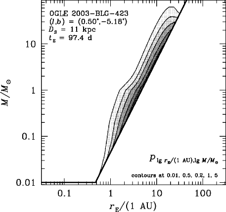
Figure 17: Bivariate probability density $p_{\lg r_{\mathrm{E}}/(1~{}\mathrm{AU}),\lg M/M_{\sun}}$ as function of the Einstein radius $r_{\mathrm{E}}$ and the lens mass $M$ for the time-scale $t_{\mathrm{E}}=97.4$ as determined by Yoo et al. (2004) for OGLE 2003-BLG-423, and the corresponding location $(l,b)=(0.50\degr,-5.18\degr)$, while a source distance $D_{\mathrm{S}}=11~{}\mathrm{kpc}$ has been assumed. The bold line marks the upper limit for $r_{\mathrm{E}}$ and the mass cut-off at $M=0.01~{}M_{\sun}$, which arises from the adopted mass spectrum.

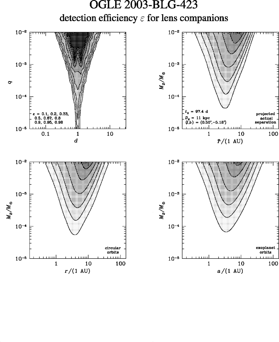
Figure 18: Detection efficiency maps resulting from MicroFUN and OGLE data collected for the event OGLE 2003-BLG-423. The top left panel shows the detection efficiency $\varepsilon_{d,q}(d,q)$ in the model parameters $(d,q)$ as calculated by Yoo et al. (2004), where the actual angular separation between the lens constituents is $d\,\theta_{\mathrm{E}}$ and $q$ denotes their mass ratio. The remaining panels show the detection efficiency as function of the physical lens properties derived using the Galaxy model described in Appendix B, using the event time-scale $t_{\mathrm{E}}=97.4~{}\mathrm{d}$ resulting from the photometric data, $D_{\mathrm{S}}=11~{}\mathrm{kpc}$ and the Galactic coordinates $(l,b)=(0.50\degr,-5.18\degr)$. All these plots refer to the secondary mass $M_{2}$, but different separations, where the top right panel shows the detection efficiency for the actual projected distance perpendicular to the line-of-sight $\hat{r}=d\,r_{\mathrm{E}}$, the bottom left planet refers to the orbital radius $r$ assuming circular orbits, and the semi-major axis $a$ is used in the bottom right panel assuming elliptical orbits with the eccentricity distribution $\Phi_{e}=(4/\pi)\,\sqrt{1-e^{2}}$ (see Appendix C). For each of the plots, contour levels are shown at $\varepsilon=0.1,0.2,0.33,0.5,0.67,0.8,0.9,0.95,0.98$. While all these contours shown up for the plot of $\varepsilon_{d,q}(d,q)$, some contours that correspond to larger detection efficiencies fall outside the displayed region for the other plots.

A given semi-major axis $a$ of the binary lens may result in different projected actual separations $\hat{r}$ depending on the spatial orientation of the orbit, the orbital phase and the orbital eccentricity. With $\Phi_{\hat{\chi}}(\hat{\chi})$ denoting the probability density of $\hat{\chi}=\hat{r}/a$ as derived in Appendix C, the detection efficiency in $(a,M_{2})$ follows as

$$\varepsilon_{a,M_{2}}(a,M_{2})=\int\limits_{0}^{{\hat{\chi}}^{\mathrm{max}}}\varepsilon_{\hat{r},M_{2}}({\hat{\chi}}\,a,M_{2})\,\Phi_{\hat{\chi}}(\hat{\chi})\,\mathrm{d}{\hat{\chi}}\,.$$ (70)

For circular orbits, the expression for $\Phi_{\hat{\chi}}(\hat{\chi})$ given by Eq. (127) yields with a variable substitution in favour of $\hat{w}=\sqrt{1-{\hat{\chi}}^{2}}$ and ${\hat{\chi}}^{\mathrm{max}}=1$

$$\varepsilon_{a,M_{2}}(a,M_{2})=\int\limits_{0}^{1}\varepsilon_{\hat{r},M_{2}}(\sqrt{1-{\hat{w}}^{2}}\;a,M_{2})\,\mathrm{d}{\hat{w}}\,.$$ (71)

Following a pilot analysis of the event OGLE 1998-BUL-14 (Albrow et al., 2000b), for which the underlying technique has been developed, the PLANET (Probing Lensing Anomalies NETwork) collaboration has calculated detection efficiency maps in the parameters $(d,q)$ for its data collected from 1995 to 1999 in order to derive upper abundance limits on planetary companions to the lens stars (Albrow et al., 2001; Gaudi et al., 2002). Detection efficiency maps have also been derived by the MPS (Microlensing Planet Search) and MOA (Microlensing Observations in Astrophysics) collaborations for the event MACHO 1998-BLG-35 (Rhie et al., 2000), and several other groups for suitable events (Tsapras et al., 2002; Bond et al., 2002; Yoo et al., 2004; Dong et al., 2005), while Tsapras et al. (2003) and Snodgrass et al. (2004) have determined planetary abundance limits from OGLE (Optical Gravitational Lens Experiment) data. The largest sensitivity to planets so far was achieved for the event MOA 2003-BLG-32/OGLE 2003-BLG-219 (Abe et al., 2004) that showed an extreme peak magnification in excess of 500. PLANET is in the progress of carrying out a new comprehensive analysis including the more recently observed events (Cassan et al., 2005), where, based on the results presented in this section, a planetary abundance $f_{a,M_{2}}(a,M_{2})$ rather than $f_{d,q}(d,q)$ is considered.

For the parameters of the event OGLE 2003-BLG-423, where the source star is located towards $(l,b)=(0.50\degr,-5.18\degr)$ and the best-fitting event time-scale assuming a point lens is $t_{\mathrm{E}}=97.4~{}\mathrm{d}$, Figure 17 shows the bivariate probability density $p_{\lg r_{\mathrm{E}}/(1~{}\mathrm{AU}),\lg M/M_{\sun}}$ as function of the Einstein radius $r_{\mathrm{E}}$ and the lens mass $M$, where $D_{\mathrm{S}}=11~{}\mathrm{kpc}$ has been assumed. The bold line marks the upper limit for $r_{\mathrm{E}}$, which corresponds to the lens being half-way between source and observer ($x=0.5$), and the mass cut-off at $M=0.01~{}M_{\sun}$, resulting from the adopted mass spectrum. As the Einstein radius $r_{\mathrm{E}}$ approaches its maximal value, $p_{\lg r_{\mathrm{E}}/(1~{}\mathrm{AU}),\lg M/M_{\sun}}$ diverges.

The detection efficiency as function of the model parameters $(d,q)$ that has been calculated by Yoo et al. (2004) based on data collected by MicroFUN (Microlensing Follow-Up Network) and OGLE for this event is shown in the top left panel of Fig. 18. Data from the OGLE survey are made available on-line as the events are progressing (Udalski, 2003), which significantly eases the assessment of their parameters and thereby allows the optimization of follow-up observations. Using the expressions presented in this section and adopting the Galaxy model described in Appendix B, corresponding detection efficiency maps in physical quantities have been determined, where the single time-scale $t_{\mathrm{E}}=97.4~{}\mathrm{d}$ has been used rather than the more exact best-fitting value for each $(d,q)$ that refers to the primary mass, and a source distance of $D_{\mathrm{S}}=11~{}\mathrm{kpc}$ has been assumed. These maps are shown in the remaining panels of Fig. 18, where the detection efficiency refers to the secondary mass $M_{2}$ and the projected actual separation $\hat{r}$, the orbital radius $r$ for circular orbits, or the semi-major axis $a$ for elliptical orbits. The distribution of the eccentricity $e$ for elliptical orbits has been chosen to be $\Phi_{e}(e)=(4/\pi)\sqrt{1-e^{2}}$, which provides a rough model of the eccentricities for planetary orbits found by radial velocity searches (see Appendix C).

All detection efficiency maps show the similar pattern of a maximum efficiency for a characteristic separation decreasing both towards smaller and larger separations and a decrease of detection efficiency towards smaller masses. As compared to the detection efficiency in the model parameters $(d,q)$, the other panels show the detection efficiency being stretched over a broader range of parameter space, so that peak detection efficiencies are reduced, while smaller values occupy wider regions. The main broadening occurs on the transition from $(d,q)$ to $(\hat{r},M_{2})$, so that the width of the distributions of the lens mass, distance, and velocity yield the dominant contribution rather than the orbital projection, which has a more moderate but highly significant effect. While the map in the projected actual separation $\hat{r}$ reflects the upper limit of the Einstein radius $r_{\mathrm{E}}$, this is smeared out by the distribution of the projection factor when considering the semi-major axis instead. The average orbital radius $r$ for circular orbits exceeds the average semi-major axis for the considered elliptic orbits, and for elliptic orbits, the detection efficiency is also stretched towards smaller $a$, with $1<\hat{\chi}=\hat{r}/a<2$ being possible. A substantial detection efficiency for small planetary masses results from the large abundance of parent stars with small masses, whereas stars much heavier than the Sun are rare, and the fact that large detection efficiencies from larger mass ratios provide substantial contributions with the finite width of the mass distribution for a given event time-scale.

8 Summary and outlook

This paper provides a comprehensive theoretical framework for the estimation of lens and source properties on the basis of the related model parameters that are estimated from the observational data. This formalism can be used to answer a large variety of questions about the nature of individual microlensing events. With the adopted Galaxy model and a source star residing in the direction of Baade’s window $(l,b)=(1\degr,-3.9\degr)$ at $D_{\mathrm{S}}=8.5~{}\mathrm{kpc}$, 35 per cent of all ongoing events (not identical with the monitored or detected ones) are caused by lenses in the Galactic disk and 65 per cent by lenses in the Galactic bulge. While the bulge lenses clearly dominate the total event rate only for very small time-scales $t_{\mathrm{E}}\la 2~{}\mathrm{d}$, the disk lenses yield the larger contribution for time-scales $2~{}\mathrm{d}\la t_{\mathrm{E}}\la 40~{}\mathrm{d}$ and $t_{\mathrm{E}}\ga 100~{}\mathrm{d}$, where the latter however yield only a small contribution to the total rate. For $2~{}\mathrm{d}\la t_{\mathrm{E}}\la 40~{}\mathrm{d}$, bulge and disk lenses yield comparable contributions. The provision of probability densities of the underlying characteristics of the lens and source system such as the lens mass $M$, the distance $D_{\mathrm{L}}$ and the effective transverse absolute velocity $v$ under the assumption of mass spectra, mass densities and velocity distributions yields the largest amount of information that can be extracted from the observations, i.e. much more than by a finite number of moments. While a mass $M\sim 0.36~{}M_{\sun}$ for $t_{\mathrm{E}}=20~{}\mathrm{d}$ is in rough agreement with estimates using a ’typical’ fractional lens distance $x$ and transverse velocity $v$, the assumed mass spectrum with a low abundance for $M\ga 1~{}M_{\sun}$ forces the expected mass to be more narrowly distributed with $t_{\mathrm{E}}$ rather than to follow the naive $M\propto t_{\mathrm{E}}^{2}$ law. In particular, there are only 1.5 decades $0.09~{}M_{\sun}\leq M\leq 3~{}M_{\sun}$ for the expected mass if time-scales $3~{}\mathrm{d}\leq t_{\mathrm{E}}\leq 150~{}\mathrm{d}$ are considered where the inclusion of one standard deviation extends this range to $0.03~{}M_{\sun}\leq M\leq 15~{}M_{\sun}$.

Additional constraints such as those resulting from a measurement of the relative proper motion between lens and source from observed finite-source effects or the relative lens-source parallax as well as upper limits on these quantities resulting from the absence of related effects can be incorporated. Explicitly one sees how uncertainties in $M$, $D_{\mathrm{L}}$, and $v$ are reduced, although the respective probability densities can also widen if the additional constraint forces the lens to assume values that fall into regions disfavoured by the given time-scale. For any set of observables, one also obtains a probability for the lens to reside in any of the potential lens populations. Unless there are sufficient constraints to yield a sharp value for the lens mass, distance, and velocity for a given set of model parameters, the uncertainties of the latter can be neglected against the broad distributions of the relevant characteristics of the lens populations and the Galaxy model uncertainties. With significant effects by annual parallax on the light curve starting at $\pi_{\mathrm{E}}\la 0.8$, such a limit can be detected in an event with time-scale $t_{\mathrm{E}}=20~{}\mathrm{d}$ with a sensitivity to an angular positional shift within $t_{\mathrm{E}}$ of $\kappa_{\pi}\,\theta_{\mathrm{E}}\sim 0.05~{}\theta_{\mathrm{E}}$, whereas $\kappa_{\pi}=1$ is reached for $t_{\mathrm{E}}\sim 90~{}\mathrm{d}$. Similarly, finite-source effects become apparent if the angular source size $\theta_{\star}$ becomes a fair fraction of the angular impact $u_{0}\,\theta_{\mathrm{E}}$ between lens and source. By requiring $u_{0}\la 2\,(\theta_{\star}/\theta_{\mathrm{E}})=2\,{\hat{\rho}}_{\star,\sun}\,(R_{\star}/R_{\sun})$, a limit ${\hat{\rho}}_{\star,\sun}\leq 0.005$ for $R_{\star}=R_{\sun}$ is detected if $u_{0}\la 0.01$, corresponding to a peak magnification $A_{0}\ga 100$, whereas an impact parameter $u_{0}\la 0.1$, corresponding to $A_{0}\ga 10$, is sufficient for $R_{\star}=10~{}R_{\sun}$.

In addition to the basic quantities, probability densities of the orbital semi-major axis and the orbital period for binary lenses, as well as of any quantity that depends on the basic characteristics, can be obtained. The bivariate probability density of the Einstein radius $r_{\mathrm{E}}$ and the lens mass $M$ together with statistics of binary orbits yields detection efficiency maps for planetary companions to the lens star as function of the planet mass $M_{2}$ and its orbital semi-major axis $a$ rather than of the model parameters $d$ and $q$, where $d\,\theta_{\mathrm{E}}$ is the actual angular separation from its parent star and $q$ is the planet-to-star mass ratio. The presented formalism has been applied to some first examples and will be used for discussing the implications of many further events. This paper explicitly shows the distributions of event properties for the binary-lens model of microlensing event OGLE 2002-BLG-099 (Jaroszyński et al., 2004), namely of the masses of the lens components and their distance from the observer, as well as of the orbital semi-major axis and period. Moreover, it shows the detection efficiency map in $(a,M_{2})$ resulting from MicroFUN and OGLE data (Yoo et al., 2004) for the event OGLE 2003-BLG-423. As a function of $(a,M_{2})$, the detection efficiency stretches over a much broader range of parameter space than for the $(d,q)$-map. In particular, this results in a larger detection efficiency for low-mass planets than one would expect from typical values.

Appendix A General probabilistic approach

Let us consider a system characterized by $k$ properties $a_{i}$ ($i=1\ldots k$) that are distributed statistically, where $\Phi_{a_{i}}(a_{1}\ldots a_{k})\,\mathrm{d}a_{i}$ gives the probability to find the property $a_{i}$ in the interval $[a_{i},a_{i}+\mathrm{d}a_{i}]$ which might depend on all $a_{1}\ldots a_{k}$. Further consider any realization of these system properties yielding a specific contribution to observed events described by a weight function $\Omega(a_{1}\ldots a_{k})$ which may be chosen appropriately to include selection effects caused by the experiment, so that the total event rate according to their statistical representation is given by

$$\Gamma(\Phi_{a_{i}}\ldots\Phi_{a_{k}};\Omega)$$

$$=\;\int\stackrel{{\scriptstyle({k})}}{{\ldots}}\int\!\Omega(a_{1}\ldots a_{k})\left\{\prod_{i=1}^{k}\Phi_{a_{i}}(a_{1}\ldots a_{k})\right\}\left\{\prod_{j=1}^{k}\mathrm{d}a_{j}\right\},$$ (72)

where the notation refers to a $k$-dimensional integral.

Hence, the probability density of the properties $a_{1}\ldots a_{k}$ among all observed events is proportional to

$$\widetilde{p}_{a_{1}\ldots a_{k}}(a_{1}\ldots a_{k};\Phi_{a_{1}}\ldots\Phi_{a_{k}},\Omega)$$

$$\qquad\quad=\;\Omega(a_{1}\ldots a_{k})\prod\limits_{i=1}^{k}\Phi_{a_{i}}(a_{1}\ldots a_{k})\,,$$ (73)

so that an appropriately normalized probability density is given by

$$p_{a_{1}\ldots a_{k}}(a_{1}\ldots a_{k};\Phi_{a_{1}}\ldots\Phi_{a_{k}},\Omega)$$

$$=\;\widetilde{p}_{a_{1}\ldots a_{k}}(a_{1}\ldots a_{k};\Phi_{a_{1}}\ldots\Phi_{a_{k}},\Omega)\;\Bigg{/}$$

$$\Bigg{/}\int\stackrel{{\scriptstyle({k})}}{{\ldots}}\int\!\widetilde{p}_{a_{1}\ldots a_{k}}(a_{1}\ldots a_{k};\Phi_{a_{1}}\ldots\Phi_{a_{k}},\Omega)\,\prod\limits_{i=1}^{k}\mathrm{d}a_{i}\,,$$ (74)

which does not depend on any constant factors in $\Omega$. This means that $p_{a_{1}\ldots a_{k}}(a_{1}\ldots a_{k};\Phi_{a_{1}}\ldots\Phi_{a_{k}},\Omega)$ is obtained by weighting the intrinsic statistical distribution $\prod_{i=1}^{k}\Phi_{a_{i}}(a_{i})$ by $\Omega(a_{1}\ldots a_{k})$ and normalizing the resulting product, so that Eq. (74) corresponds to Bayes’ theorem.

A specific event involves a set of $n$ observed parameters $f_{l}(a_{1}\ldots a_{k})$, where $l=1\ldots{}n$, which in general depend on the $k$ basic underlying properties $a_{i}$, but are not necessarily identical to these. With specific realizations $f_{l}^{(0)}$ for an observed event, the event rate can be written as integral over these realizations

$$\Gamma(\Phi_{a_{i}}\ldots\Phi_{a_{k}},\Omega)$$

$$=\;\int\stackrel{{\scriptstyle({n})}}{{\ldots}}\int\!\gamma_{f_{1}\ldots f_{n}}(f_{1}^{(0)}\ldots f_{n}^{(0)};\Phi_{a_{i}}\ldots\Phi_{a_{k}},\Omega)\;\times$$

$$\times\;\prod\limits_{l=1}^{n}\,\mathrm{d}f_{l}^{(0)}$$ (75)

with the event rate density

$$\gamma_{f_{1}\ldots f_{n}}(f_{1}^{(0)}\ldots f_{n}^{(0)};\Phi_{a_{i}}\ldots\Phi_{a_{k}},\Omega)$$

$$=\;\int\stackrel{{\scriptstyle({k})}}{{\ldots}}\int\!\Omega(a_{1}\ldots a_{k})\left\{\prod\limits_{l=1}^{n}\delta\left(f_{l}(a_{1}\ldots a_{k})-f_{l}^{(0)}\right)\right\}\;\times$$

$$\times\;\left\{\prod\limits_{i=1}^{k}\Phi_{a_{i}}(a_{i})\right\}\,\left\{\prod\limits_{j=1}^{k}\mathrm{d}a_{j}\right\}\,,$$ (76)

so that the corresponding probability density of the basic properties $a_{1}\ldots a_{k}$ is given by

$$p^{(0)}_{a_{1}\ldots a_{k}}(a_{1}\ldots a_{k},f_{1}^{(0)}\ldots f_{n}^{(0)};\Phi_{a_{1}}\ldots\Phi_{a_{k}},\Omega)$$

$$=[\gamma_{f_{1}\ldots f_{n}}(f_{1}^{(0)}\ldots f_{n}^{(0)};\Phi_{a_{i}}\ldots\Phi_{a_{k}},\Omega)]^{-1}\;\times$$

$$\times\;\Omega(a_{1}\ldots a_{k})\bigg{\{}\prod\limits_{l=1}^{n}\delta\left(f_{l}(a_{1}\ldots a_{k})-f_{l}^{(0)}\right)\bigg{\}}\;\times$$

$$\times\;\bigg{\{}\prod\limits_{i=1}^{k}\Phi_{a_{i}}(a_{i})\bigg{\}}\,,$$ (77)

while the probability density of a single property $a_{r}$ reads

$$p^{(0)}_{a_{r}}(a_{r};f_{1}^{(0)}\ldots f_{n}^{(0)};\Phi_{a_{1}}\ldots\Phi_{a_{k}},\Omega)$$

$$=[\gamma_{f_{1}\ldots f_{n}}(f_{1}^{(0)}\ldots f_{n}^{(0)};\Phi_{a_{i}}\ldots\Phi_{a_{k}},\Omega)]^{-1}\;\times$$

$$\times\;\int\stackrel{{\scriptstyle({k-1})}}{{\ldots}}\int\!\Omega(a_{1}\ldots a_{k})\bigg{\{}\prod\limits_{l=1}^{n}\delta\left(f_{l}(a_{1}\ldots a_{k})-f_{l}^{(0)}\right)\bigg{\}}\;\times$$

$$\times\;\bigg{\{}\prod\limits_{i=1}^{k}\Phi_{a_{i}}(a_{i})\,\bigg{\}}\,\bigg{\{}\prod\limits_{j=1\atop j\neq r}^{k}\mathrm{d}a_{j}\bigg{\}}\,.$$ (78)

If the observables $f_{1}\ldots f_{n}$ for one or more events follow a distribution $\Psi_{f_{1}\ldots f_{n}}(f_{1}\ldots f_{n})$, the probability density of the basic properties $a_{1}\ldots a_{k}$ arises from an integral over the probability density $p^{(0)}$ for the fixed values $f_{1}^{(0)}\ldots f_{n}^{(0)}$, given by Eq. (77), as

$$p_{a_{1}\ldots a_{k}}^{\psi}(a_{1}\ldots a_{k};\Phi_{a_{1}}\ldots\Phi_{a_{k}},\Omega)$$

$$=\;\int\stackrel{{\scriptstyle({n})}}{{\ldots}}\int\!p^{(0)}_{a_{1}\ldots a_{k}}(a_{1}\ldots a_{k},f_{1}\ldots f_{n};\Phi_{a_{1}}\ldots\Phi_{a_{k}},\Omega)\;\times$$

$$\times\;\Psi_{f_{1}\ldots f_{n}}(f_{1}\ldots f_{n})\,\prod_{l=1}^{n}\mathrm{d}f_{l}\,.$$ (79)

If the observables are statistically independent, their distribution factorizes as $\Psi_{f_{1}\ldots f_{n}}(f_{1}\ldots f_{n})=\prod_{l=1}^{n}\Psi_{f_{l}}(f_{l})$. While fixed values of $f_{l}$ correspond to the distribution $\Psi_{f_{l}}(f_{l})=\delta(f_{l}-f_{l}^{(0)})$, distributions around a central value $f_{l}^{(0)}$ with a standard deviation $\sigma_{f_{l}}$ can be approximated by the Gaussian distribution

$$\Psi_{f_{l}}^{\mathrm{Gauss}}(f_{l})=\frac{1}{\sqrt{2\pi}\sigma_{f_{l}}}\,\exp\left\{-\frac{\left(f_{l}-f_{l}^{(0)}\right)^{2}}{2\sigma_{f_{l}}^{2}}\right\}\,.$$ (80)

In case the $n$ observables ${\mn@boldsymbol{f}}=(f_{1},\ldots,f_{n})$ are correlated, $\Psi_{f_{1}\ldots f_{n}}(f_{1}\ldots f_{n})$ can be modelled as a multivariate Gaussian distribution

$$\Psi_{f_{1}\ldots f_{n}}(f_{1}\ldots f_{n})=\frac{1}{(2\pi)^{n/2}\,|{\cal C}|^{1/2}}\;\times$$

$$\times\;\exp\left\{-\frac{1}{2}\,\left(\mn@boldsymbol{f}-{\mn@boldsymbol{f}}^{(0)}\right)^{\mathrm{T}}{\cal C}^{-1}\left(\mn@boldsymbol{f}-{\mn@boldsymbol{f}}^{(0)}\right)\right\}\,,$$ (81)

where ${\cal C}^{-1}$ is the inverse and $|\cal C|$ is the determinant of the covariance matrix $\cal C$, and ${\mn@boldsymbol{f}}^{(0)}=(f_{1}^{(0)},\ldots,f_{n}^{(0)})$.

The moments of any property $g(a_{1}\ldots a_{k})$ for fixed values of the observables $f_{1}^{(0)}\ldots f_{n}^{(0)}$ follow from the expectation values

$${\left\langle g^{\beta}(a_{1}\ldots a_{k})\right\rangle}^{(0)}=\int\stackrel{{\scriptstyle({k})}}{{\ldots}}\int\!g^{\beta}(a_{1}\ldots a_{k})\;\times$$

$$\times\;p^{(0)}_{a_{1}\ldots a_{k}}(a_{1}\ldots a_{k},f_{1}^{(0)}\ldots f_{n}^{(0)};\Phi_{a_{1}}\ldots\Phi_{a_{k}},\Omega)\;\times$$

$$\times\;\prod\limits_{i=1}^{k}\mathrm{d}a_{i}\,,$$ (82)

and for a distribution $\Psi_{f_{1}\ldots f_{n}}$, one finds in analogy to Eq. (79)

$${\left\langle g^{\beta}(a_{1}\ldots a_{k})\right\rangle}^{\Psi}=\int\stackrel{{\scriptstyle({n})}}{{\ldots}}\int\!\ {\left\langle g^{\beta}(a_{1}\ldots a_{k})\right\rangle}^{(0)}\;\times$$

$$\times\;\Psi_{f_{1}\ldots f_{n}}(f_{1}\ldots f_{n})\,\prod_{l=1}^{n}\mathrm{d}f_{l}\,,$$ (83)

where interchanging the integrations over $\mathrm{d}a_{1}\ldots\mathrm{d}a_{k}$ and over $\mathrm{d}f_{1}\ldots\mathrm{d}f_{n}$ yields the equivalent expression

$${\left\langle g^{\beta}(a_{1}\ldots a_{k})\right\rangle}^{\Psi}=\int\stackrel{{\scriptstyle({k})}}{{\ldots}}\int\!g^{\beta}(a_{1}\ldots a_{k})\;\times$$

$$\times\;p^{\Psi}_{a_{1}\ldots a_{k}}(a_{1}\ldots a_{k},f_{1}^{(0)}\ldots f_{n}^{(0)};\Phi_{a_{1}}\ldots\Phi_{a_{k}},\Omega)\;\times$$

$$\times\;\prod\limits_{i=1}^{k}\mathrm{d}a_{i}\,.$$ (84)

In particular, the standard deviation is given by

$$\sigma_{g}=\sqrt{\left\langle g^{2}(a_{1}\ldots a_{k})\right\rangle-\left\langle g(a_{1}\ldots a_{k})\right\rangle^{2}}\,.$$ (85)

Beyond the moments, one finds the complete probability density of a general property $g(a_{1}\ldots a_{k})$ for fixed values of the observables $f_{1}^{(0)}\ldots f_{n}^{(0)}$ to be

$$p^{(0)}_{g}(g;f_{1}^{(0)}\ldots f_{n}^{(0)};\Phi_{a_{1}}\ldots\Phi_{a_{k}},\Omega)$$

$$=[\gamma_{f_{1}\ldots f_{n}}(f_{1}^{(0)}\ldots f_{n}^{(0)};\Phi_{a_{i}}\ldots\Phi_{a_{k}},\Omega)]^{-1}\;\times$$

$$\times\;\int\stackrel{{\scriptstyle({k})}}{{\ldots}}\int\!\Omega(a_{1}\ldots a_{k})\,\delta(g-g(a_{1}\ldots a_{k}))\;\times$$

$$\times\;\bigg{\{}\prod\limits_{l=1}^{n}\delta\left(f_{l}(a_{1}\ldots a_{k})-f_{l}^{(0)}\right)\bigg{\}}\bigg{\{}\prod\limits_{i=1}^{k}\Phi_{a_{i}}(a_{i})\,\mathrm{d}a_{i}\bigg{\}}\,,$$ (86)

while for a distribution $\Psi_{f_{1}\ldots f_{n}}$, one obtains

$$p_{g}^{\Psi}(g;\Phi_{a_{1}}\ldots\Phi_{a_{k}},\Omega)$$

$$=\;\int\stackrel{{\scriptstyle({n})}}{{\ldots}}\int\!p^{(0)}_{g}(g,f_{1}\ldots f_{n};\Phi_{a_{1}}\ldots\Phi_{a_{k}},\Omega)\;\times$$

$$\times\;\Psi_{f_{1}\ldots f_{n}}(f_{1}\ldots f_{n})\,\prod_{l=1}^{n}\mathrm{d}f_{l}\,.$$ (87)

It is important to distinguish carefully the different quantities that have been defined in this section. The system properties $a_{1}\ldots a_{k}$ are distributed statistically among the population according to $\Phi_{a_{1}}\ldots\Phi_{a_{k}}$. With $\Omega(a_{1}\ldots a_{k})$ being the weight of any realization to the number of produced events, one expects $a_{1}\ldots a_{k}$ being distributed as $p_{a_{1}\ldots a_{k}}(a_{1}\ldots a_{k};\Phi_{a_{1}}\ldots\Phi_{a_{k}},\Omega)$ among all events. For a given event, with a set of observables $f_{1}(a_{1}\ldots a_{k})\ldots f_{n}(a_{1}\ldots a_{k})$ being realized as $f_{1}^{(0)}\ldots f_{n}^{(0)}$, one infers a stochastical probability density $p^{(0)}_{a_{1}\ldots a_{k}}(a_{1}\ldots a_{k},f_{1}^{(0)}\ldots f_{n}^{(0)};\Phi_{a_{1}}\ldots\Phi_{a_{k}},\Omega)$ of $a_{1}\ldots a_{k}$ or $p_{g}^{(0)}(g,f_{1}^{(0)}\ldots f_{n}^{(0)};\Phi_{a_{1}}\ldots\Phi_{a_{k}},\Omega)$ of any specific property $g(a_{1}\ldots a_{k})$, which does not need to be an observable $f_{l}$ or a basic property $a_{j}$. Finally, one can consider the observables $f_{1}\ldots f_{n}$ to follow a stochastical distribution for a single event and/or a statistical distribution from several events, namely $\Psi_{f_{1}\ldots f_{n}}$ yielding the probability densities $p_{a_{1}\ldots a_{k}}^{\Psi}(a_{1}\ldots a_{k};\Phi_{a_{1}}\ldots\Phi_{a_{k}},\Omega)$ or $p_{g}^{\Psi}(g,\Phi_{a_{1}}\ldots\Phi_{a_{k}},\Omega)$.

Appendix B Model of the Galaxy

B.1 Mass spectrum

Table 9: Coefficients for the mass laws for different parts of the mass spectrum (following Chabrier (2003))

	$\lg(M_{\mathrm{min}}/M_{\sun})$	$\lg(M_{\mathrm{max}}/M_{\sun})$	$\alpha$	$\lg(M_{\mathrm{c}}/M_{\sun})$	$\sigma_{\mathrm{c}}$
disk	$-2.0$	$-0.7$	$-0.2$	—	—
	$-0.7$	$0.0$	—	$-1.102$	$0.69$
	$0.0$	$0.54$	$4.37$	—	—
	$0.54$	$1.26$	$3.53$	—	—
	$1.26$	$1.8$	$2.11$	—	—
bulge	-2.0	-0.155	—	-0.658	0.33
	-0.155	1.8	1.3	—	—

For $M_{\mathrm{min}}\leq M\leq M_{\mathrm{max}}$, either a power-law mass function $\hat{\Phi}_{\lg(M/M_{\sun})}[\lg(M/M_{\sun})]\propto(M/M_{\sun})^{-\alpha}$ or a Gaussian distribution $\hat{\Phi}_{\lg(M/M_{\sun})}[\lg(M/M_{\sun})]\propto\exp\{-0.5\,[\lg(M/M_{\sun})-\lg(M_{\mathrm{c}}/M_{\sun})]^{2}/(\sigma_{\mathrm{c}})^{2}\}$ is adopted.

Figure 19: Adopted mass function $\hat{\Phi}_{\lg M/M_{\sun}}\propto M^{-1}\,\Phi_{\lg M/M_{\sun}}$ for lens objects in the Galactic disk or bulge whose parameters are listed in Table 9.

While the mass spectrum $\Phi_{M}(M)$ as defined by Eq. (4) gives the decomposition of the mass density into objects with mass in the range $[M,M+\mathrm{d}M]$, the decomposition of the number density is given by the mass function $\hat{\Phi}_{M}(M)\propto M^{-1}\,\Phi_{M}(M)$. As pointed out e.g. in the review of Chabrier (2003), the mass function $\hat{\Phi}_{\lg(M/M_{\sun})}$ can be fairly well approximated piecewise by different kinds of analytic functions. In particular, for selected ranges $M_{\mathrm{min}}^{(i)}\leq M\leq M_{\mathrm{max}}^{(i)}$, one may consider a power-law mass spectrum in $M$, i.e.

$$\hat{\Phi}^{(i)}_{\lg(M/M_{\sun})}[\lg(M/M_{\sun})]\propto(M/M_{\sun})^{-\alpha^{(i)}}$$ (88)

with the power index $\alpha^{(i)}$, or a Gaussian distribution in $\lg(M/M_{\sun})$, i.e.

$$\hat{\Phi}^{(i)}_{\lg(M/M_{\sun})}[\lg(M/M_{\sun})]\;\propto$$

$$\propto\;\exp\left\{-0.5\,[\lg(M/M_{\sun})-\lg(M_{\mathrm{c}}^{(i)}/M_{\sun})]^{2}/(\sigma_{\mathrm{c}}^{(i)})^{2}\right\}$$ (89)

with the characteristic mass $M_{\mathrm{c}}^{(i)}$ and the width of the distribution $\sigma_{\mathrm{c}}^{(i)}$. The proportionality factors thereby have to be chosen so that the mass spectrum $\Phi_{\lg(M/M_{\sun})}$ is continuous at all $M_{\mathrm{max}}^{(i)}=M_{\mathrm{min}}^{(i+1)}$, and its integral over all $\lg(M/M_{\sun})$ becomes unity. The choice for the parameters corresponding to different selected mass ranges for disk or bulge lenses following Chabrier (2003), that is adopted for this paper, is shown in Table 9, and the corresponding mass function $\hat{\Phi}_{\lg(M/M_{\sun})}(\lg(M/M_{\sun}))$ is shown in Fig. 19.

B.2 Mass density

The view from the observer to the source is reflected by a coordinate system with a basis $(\mn@boldsymbol{e}_{x},\mn@boldsymbol{e}_{y},\mn@boldsymbol{e}_{z})$ where $\mn@boldsymbol{e}_{x}$ points from the observer to the source, while $\mn@boldsymbol{e}_{y}$ and $\mn@boldsymbol{e}_{z}$ span a plane perpendicular to the line-of-sight. For describing properties of the Galaxy, however, it is more appropriate to refer to the galactic coordinates $(D_{\mathrm{L}},l,b)$ which are the spherical coordinates that refer to the basis $({\mn@boldsymbol{E}}_{X},{\mn@boldsymbol{E}}_{Y},{\mn@boldsymbol{E}}_{Z})$, where ${\mn@boldsymbol{E}}_{X}$ points to the Galactic centre $(l,b)=(0\degr,0\degr)$, ${\mn@boldsymbol{E}}_{Y}$ towards the direction of local circular motion $(l,b)=(90\degr,0\degr)$, and ${\mn@boldsymbol{E}}_{Z}$ towards Galactic North $b=90\degr$, so that ${\mn@boldsymbol{X}}=D_{\mathrm{L}}\,(\cos l\cos b,\sin l\cos b,\sin b)$. The basis $(\mn@boldsymbol{e}_{x},\mn@boldsymbol{e}_{y},\mn@boldsymbol{e}_{z})$ arises from $({\mn@boldsymbol{E}}_{X},{\mn@boldsymbol{E}}_{Y},{\mn@boldsymbol{E}}_{Z})$ by a rotation ${\cal R}({\mn@boldsymbol{E}}_{Z};l)$ around ${\mn@boldsymbol{E}}_{Z}$ by the angle $l$ and a subsequent rotation ${\cal R}(-{\cal R}({\mn@boldsymbol{E}}_{Z};l){\mn@boldsymbol{E}}_{Y};b)$ around $-{\cal R}({\mn@boldsymbol{E}}_{Z};l){\mn@boldsymbol{E}}_{Y}$ by the angle $b$, i.e. ${\mn@boldsymbol{e}}_{i}=\sum_{j}{\cal T}_{ij}(l,b){\mn@boldsymbol{E}}_{j}$, where

$${\cal T}(l,b) = \left(\begin{array}[]{ccc}\cos b&0&\sin b\\ 0&1&0\\ -\sin b&0&\cos b\end{array}\right)\,\left(\begin{array}[]{ccc}\cos l&\sin l&0\\ -\sin l&\cos l&0\\ 0&0&1\end{array}\right)$$ (96)

$$= \left(\begin{array}[]{ccc}\cos l\cos b&\sin l\cos b&\sin b\\ -\sin l&\cos l&0\\ -\cos l\sin b&-\sin l\sin b&\cos b\end{array}\right)\,,$$ (100)

so that vector components transform as $\mn@boldsymbol{x}=\left({\cal T}^{-1}\right)^{\mathrm{T}}(l,b)\,{\mn@boldsymbol{X}}={\cal T}(l,b)\,{\mn@boldsymbol{X}}$ or ${\mn@boldsymbol{X}}={\cal T}^{-1}(l,b)\,{\mn@boldsymbol{x}}={\cal T}^{\mathrm{T}}(l,b)\,{\mn@boldsymbol{x}}$.

The density of matter in the Galaxy is more easily expressed in coordinate frames whose origins are at the Galactic centre rather than at the position of the Sun. Just by subtracting the corresponding difference location vector, one finds for such a system with the fractional lens distance $x\equiv D_{\mathrm{L}}/D_{\mathrm{S}}$ and the galactic coordinates $(l,b)$ of the source star:

$$\hat{X} = X-R_{0}\;=\;x\,D_{\mathrm{S}}\,\cos l\,\cos b-R_{0}\,,$$

$$\hat{Y} = Y\;=\;x\,D_{\mathrm{S}}\,\sin l\,\cos b\,,$$

$$\hat{Z} = Z\;=\;x\,D_{\mathrm{S}}\,\sin b\,.$$ (101)

Hence, the cylindrical distance from the Galactic centre is

$$R = \sqrt{{\hat{X}}^{2}+{\hat{Y}}^{2}}$$ (102)

$$= R_{0}\,\sqrt{[\cos l-x\,(D_{\mathrm{S}}/R_{0})\,\cos b]^{2}+\sin^{2}l}\,,$$

while the spherical distance reads

$$r = \sqrt{{\hat{X}}^{2}+{\hat{Y}}^{2}+{\hat{Z}}^{2}}$$ (103)

$$= \sqrt{R_{0}^{2}+x^{2}D_{\mathrm{S}}^{2}-2\,xD_{\mathrm{S}}R_{0}\cos l\cos b}\,.$$

Figure 20: Weighted probability density $\kappa\,\Phi_{x}(x)$ of the fractional lens distance $x=D_{\mathrm{L}}/D_{\mathrm{S}}$ for two different positions of the source, and lenses in the Galactic disk or bulge. The weight factors are given by $\kappa^{\mathrm{disk}}=\Sigma^{\mathrm{disk}}/(\Sigma^{\mathrm{disk}}+\Sigma^{\mathrm{bulge}})$ and $\kappa^{\mathrm{bulge}}=\Sigma^{\mathrm{bulge}}/(\Sigma^{\mathrm{disk}}+\Sigma^{\mathrm{bulge}})$, so that $\kappa\,\Phi_{x}(x)$ reflects the mass density, where $\int_{0}^{1}[\kappa^{\mathrm{disk}}\Phi_{x}^{\mathrm{disk}}+\kappa^{\mathrm{bulge}}\Phi_{x}^{\mathrm{bulge}}]\,\mathrm{d}x=1$, i.e. $\kappa^{\mathrm{disk}}+\kappa^{\mathrm{bulge}}=1$. While $\kappa^{\mathrm{disk}}\sim 2\times 10^{-5}$ for the source in the spiral arm, one finds $\kappa^{\mathrm{disk}}=0.33$ and $\kappa^{\mathrm{bulge}}=0.67$ for the bulge source.

As chosen by Grenacher et al. (1999), the mass density of the disk is modelled by two double-exponential disks, following Bahcall, Soneira & Schmidt (1983) and Gilmore, Wyse & Kuijken (1989), where

$$\rho^{\mathrm{disk}}(R,Z)=0.5\,\exp\left(-\frac{R-R_{0}}{h}\right)\;\times$$

$$\times\;\left[\frac{\Sigma_{\mathrm{thin}}}{H_{\mathrm{thin}}}\exp\left(-\frac{|Z|}{H_{\mathrm{thin}}}\right)+\frac{\Sigma_{\mathrm{thick}}}{H_{\mathrm{thick}}}\exp\left(-\frac{|Z|}{H_{\mathrm{thick}}}\right)\right]$$ (104)

with $h=3.5~{}\mathrm{kpc}$ being the scale length in the galactic plane, while $H_{\mathrm{thin}}=0.3~{}\mathrm{kpc}$ and $H_{\mathrm{thick}}=1.0~{}\mathrm{kpc}$ are the scale lengths of a thin and a thick disk perpendicular to the galactic plane, and the corresponding column mass densities are $\Sigma_{\mathrm{thin}}=25~{}M_{\sun}\,\mathrm{pc}^{-2}$ and $\Sigma_{\mathrm{thick}}=35~{}M_{\sun}\,\mathrm{pc}^{-2}$.

Similar to the discussion of Han & Gould (1995b, a) and Grenacher et al. (1999), let us adopt a model of a barred bulge based on the COBE data (Dwek et al., 1995), which is tilted by an angle $\theta=20\degr$ with respect to the direction of the Galactic centre, so that coordinates along its main axes with origin at the Galactic centre are given by

$$\hat{X}^{\prime} = \hat{X}\cos\theta+\hat{Y}\sin\theta\,,$$

$$\hat{Y}^{\prime} = -\hat{X}\sin\theta+\hat{Y}\cos\theta\,,$$

$$\hat{Z}^{\prime} = \hat{Z}\,.$$ (105)

In these coordinates, the mass density of the Galactic bulge can be expressed by

$$\rho^{\mathrm{bulge}}(\hat{X}^{\prime},\hat{Y}^{\prime},\hat{Z}^{\prime})=\rho^{\mathrm{bulge}}_{0}\,\exp\left\{-s^{2}/2\right\}\,,$$ (106)

where

$$s^{2}=\sqrt{\left[\left(\hat{X}^{\prime}/a\right)^{2}+\left(\hat{Y}^{\prime}/b\right)^{2}\right]^{2}+\left(\hat{Z}^{\prime}/c\right)^{4}}$$ (107)

with $a=1.58~{}\mathrm{kpc}$, $b=0.62~{}\mathrm{kpc}$, and $c=0.43~{}\mathrm{kpc}$. A total mass $M_{\mathrm{bulge}}=1.8\times 10^{10}~{}M_{\sun}$ implies $\rho^{\mathrm{bulge}}_{0}=M_{\mathrm{bulge}}/(6.57\,\pi\,abc)=2.1\times 10^{9}~{}M_{\sun}\,\mathrm{kpc}^{-3}$.

For a source in the Galactic bulge towards Baade’s window at $(l,b)=(1\degr,-3.9\degr)$ at a distance $D_{\mathrm{S}}=8.5~{}\mathrm{kpc}$ as well as for a source in the Carina spiral arm at $(l,b)=(290.8\degr,-0.98\degr)$ and a distance $D_{\mathrm{S}}=6.8~{}\mathrm{kpc}$ as example for an off-bulge target, the weighted probability densities $\kappa\,\Phi_{x}(x)$ of the fractional lens distance $x\equiv D_{\mathrm{L}}/D_{\mathrm{S}}$ are shown in Fig. 20. The weight factors $\kappa^{\mathrm{disk}}=\Sigma^{\mathrm{disk}}/(\Sigma^{\mathrm{disk}}+\Sigma^{\mathrm{bulge}})$ and $\kappa^{\mathrm{bulge}}=\Sigma^{\mathrm{bulge}}/(\Sigma^{\mathrm{disk}}+\Sigma^{\mathrm{bulge}})$ have been chosen so that $\int_{0}^{1}[\kappa^{\mathrm{disk}}\Phi_{x}^{\mathrm{disk}}+\kappa^{\mathrm{bulge}}\Phi_{x}^{\mathrm{bulge}}]\,\mathrm{d}x=1$ and $\kappa^{\mathrm{disk}}+\kappa^{\mathrm{bulge}}=1$. Not surprisingly, the contribution of bulge lenses is negligible for a source in the spiral arm, where for the chosen parameters, $\kappa^{\mathrm{bulge}}=2\times 10^{-5}$. In contrast, for the bulge source, one finds contributions of comparable order, where $\kappa^{\mathrm{disk}}=0.33$ and $\kappa^{\mathrm{bulge}}=0.67$. While the lens mass density for the source in the spiral arm shows a broad distribution favouring smaller lens distances, one finds a moderate increase with distance for disk lenses and a source in the Galactic bulge, while bulge lenses yields significant contributions only for $x\ga 0.6$.

B.3 Effective transverse velocity

The effective transverse velocity in a plane at the lens distance $D_{\mathrm{L}}=x\,D_{\mathrm{S}}$ perpendicular to the line-of-sight is given by

$$\mn@boldsymbol{v}(x)=\mn@boldsymbol{v}_{\mathrm{L}}-x\,\mn@boldsymbol{v}_{\mathrm{S}}-(1-x)\,\mn@boldsymbol{v}_{\mathrm{O}}\,,$$ (108)

where $\mn@boldsymbol{v}_{\mathrm{L}}$, $\mn@boldsymbol{v}_{\mathrm{S}}$, and $\mn@boldsymbol{v}_{\mathrm{O}}$ denote the perpendicular velocities of the lens, source, or observer, respectively. Let us consider an expectation value ${\mn@boldsymbol{v}}^{0}=\left\langle\mn@boldsymbol{v}\right\rangle$, and the source and lens velocities follow Gaussian distributions, where isotropic velocity dispersions are assumed for both the Galactic disk and bulge. While the introduction of anisotropies heavily complicates both the discussion and the calculation, the results are only marginally affected, and the arising differences do not exceed those resulting from uncertainties in the velocity dispersions themselves. Discussions of anisotropic velocity dispersions must not miss the non-diagonal elements of the velocity dispersion tensor for directions that do not coincide with the main axes of the velocity dispersion ellipsoid.

In this paper, values of $\sigma^{\mathrm{disk}}=30~{}\mathrm{km}\,\mathrm{s}^{-1}$ for the Galactic disk and $\sigma^{\mathrm{bulge}}=100~{}\mathrm{km}\,\mathrm{s}^{-1}$ for the Galactic bulge have been adopted. Therefore, for bulge sources, the total velocity dispersion is $\sigma(x)=\sqrt{1+x^{2}}\,\sigma^{\mathrm{bulge}}$ for bulge lenses or $\sigma(x)=\sqrt{x^{2}\,\left(\sigma^{\mathrm{bulge}}\right)^{2}+\left(\sigma^{\mathrm{disk}}\right)^{2}}$ for disk lenses, while for disk sources, where the lens also resides in the Galactic disk, $\sigma(x)=\sqrt{1+x^{2}}\,\sigma^{\mathrm{disk}}$.

The probability density $\Phi_{v}(v)$ of the absolute effective velocity therefore takes the form

$$\Phi_{v}(v,x)$$

$$=\frac{v}{2\pi\,[\sigma(x)]^{2}}\int\limits_{0}^{2\pi}\,\exp\left\{-\frac{1}{2\,[\sigma(x)]^{2}}\,\left(\mn@boldsymbol{v}-{\mn@boldsymbol{v}}^{0}(x)\right)^{2}\right\}\,\mathrm{d}\varphi$$

$$=\frac{v}{2\pi\,[\sigma(x)]^{2}}\,\exp\left\{-\frac{v^{2}+[v^{0}(x)]^{2}}{2\,[\sigma(x)]^{2}}\right\}\;\times$$

$$\qquad\times\;\int\limits_{0}^{2\pi}\exp\left\{\frac{v\,v^{0}(x)}{[\sigma(x)]^{2}}\,\cos\varphi\right\}\,\mathrm{d}\varphi$$

$$=\frac{v}{[\sigma(x)]^{2}}\,\exp\left\{-\frac{v^{2}+[v^{0}(x)]^{2}}{2\,[\sigma(x)]^{2}}\right\}\,I_{0}\left(\frac{v\,v^{0}(x)}{[\sigma(x)]^{2}}\right)$$ (109)

with $\varphi$ being the angle between $\mn@boldsymbol{v}$ and $\mn@boldsymbol{v}^{0}(x)$, $v=|\mn@boldsymbol{v}|$, $v^{0}(x)=|\mn@boldsymbol{v}^{0}(x)|$, and $I_{0}(\eta)$ denoting the modified Bessel function of the first kind to the order zero.

Hence, with dimensionless $\zeta=v/v_{\mathrm{c}}$, $\zeta^{0}(x)=v^{0}(x)/v_{\mathrm{c}}$, and $\hat{\sigma}(x)=\sigma(x)/v_{\mathrm{c}}$, one finds

$$\Phi_{\zeta}(\zeta,x)$$

$$=\frac{\zeta}{[\hat{\sigma}(x)]^{2}}\,\exp\left\{-\frac{\zeta^{2}+[\zeta^{0}(x)]^{2}}{2\,[\hat{\sigma}(x)]^{2}}\right\}\,I_{0}\left(\frac{\zeta\,\zeta^{0}(x)}{[\hat{\sigma}(x)]^{2}}\right)\,.$$ (110)

While the direction of the velocity vector for Bulge objects is purely random, disk lenses as well as the Sun perform a systematic rotation around the Galactic centre with a velocity $v_{\mathrm{circ}}(R)$ depending on the cylindrical distance $R$. With $R$ given by Eq. (102), the systematic lens motion reads

$$v_{\mathrm{L},y}^{0}(x) = v_{\mathrm{circ}}(R)\;\frac{R_{0}\,\cos l-x\,D_{\mathrm{S}}\,\cos b}{R}\,,$$

$$v_{\mathrm{L},z}^{0}(x) = v_{\mathrm{circ}}(R)\;\frac{R_{0}\,\sin l\sin b}{R}\,\,.$$ (111)

The rotation velocity can be effectively described by the model introduced by Navarro, Frenk & White (1997), where the mass density is given by

$$\rho(x)\propto\frac{1}{r(r+r_{\mathrm{S}})^{2}}\,,$$ (112)

so that with

$$M(r)=4\pi\int\limits_{0}^{r}\rho(\tilde{r})\,{\tilde{r}}^{2}\,\mathrm{d}{\tilde{r}}$$ (113)

and $v_{\mathrm{circ}}(r)=[G\,M(r)/r]^{1/2}$, one finds

$$v_{\mathrm{circ}}(R)=v_{\mathrm{circ}}(R_{0})\,f^{0}_{\mathrm{NFW}}\;\times$$

$$\times\;\sqrt{\frac{R_{0}}{R}}\,\sqrt{\ln\left[1+R/r_{\mathrm{S}}\right]-\frac{R}{R+r_{\mathrm{S}}}}\,,$$ (114)

where the choices $v_{\mathrm{circ}}(R_{0})=220\,\mathrm{km}\,\mathrm{s}^{-1}$ for the reference distance $R_{0}=8.5~{}\mathrm{kpc}$ and $r_{\mathrm{S}}=20\,\mathrm{kpc}$ yield $f^{0}_{\mathrm{NFW}}=4.23$.

Figure 21: Probability density $\Phi_{\lg\zeta}(\lg\zeta)=\zeta\,\ln 10\;\Phi_{\zeta}(\zeta)$, where $\zeta=v/v_{\mathrm{c}}$. The two panels correspond to different positions of the source, where the lens is either located in the Galactic disk or bulge at a fractional lens distance $x\equiv D_{\mathrm{L}}/D_{\mathrm{S}}$. The bulge population is not considered for the source in the spiral arm, because its contribution to the event rate can be neglected.

With respect to the rest frame of the Galaxy, the Sun, located at a distance $R_{0}$ from the Galactic centre, shows a peculiar motion ${\mn@boldsymbol{V}_{\sun}}=(V_{{\sun},X},V_{{\sun},Y},V_{{\sun},Z})=(9,12,7)\,\mathrm{km}\,\mathrm{s}^{-1}$ on top of the circular motion of the Galactic disk of ${\mn@boldsymbol{V}_{{\sun},\mathrm{circ}}}=(0,v_{\mathrm{circ}}(R_{0}),0)$ with $v_{\mathrm{circ}}(R_{0})=220\,\mathrm{km}\,\mathrm{s}^{-1}$.

One also might consider including the velocity of the Earth of $v_{\oplus}=30~{}\mathrm{km}\,\mathrm{s}^{-1}$. While for event time-scales $t_{\mathrm{E}}\ll 1~{}\mathrm{yr}$, this velocity is approximately constant (and roughly equivalent to the value at the closest angular approach between lens and source), and to next order, the acceleration of the Earth’s motion can be included in the model of the observed light curve by means of additional parameters, the full annual modulation affects the light curve for longer time-scales and this parallax effect needs to be accounted for. In the last case, however, there is no effective Earth’s velocity that contributes to $v$. For the calculations in this paper, the velocity of the Earth is neglected, so that with ${\cal T}(l,b)$ from Eq. (100), one obtains ${\mn@boldsymbol{v}}^{0}_{\mathrm{O}}={\cal T}(l,b)(\mn@boldsymbol{V}_{\sun,\mathrm{circ}}+\mn@boldsymbol{V}_{\sun})$ or

$$v^{0}_{\mathrm{O},y}=-\sin l\,V_{\sun,X}+\cos l\,\left[V_{\sun,Y}+v_{\mathrm{circ}}(R_{0})\right]\,,$$

$$v^{0}_{\mathrm{O},z}=-\cos l\sin b\,V_{\sun,X}\;-$$

$$-\;\sin l\sin b\,\left[V_{\sun,Y}+v_{\mathrm{circ}}(R_{0})\right]+\cos b\,V_{\sun,Z}\,.$$ (115)

Fig. 21 shows the distribution of the effective velocity for a source in the Carina spiral arm or in the Galactic bulge for either bulge or disk lenses, where the same parameters as for the distribution of the lens distance shown in Fig. 20 have been adopted. In consistence with the latter, ’typical’ values of $x=0.85$ for the source in the Galactic bulge or $x=0.35$ for the source in the spiral arm have been chosen. The shift towards larger velocities for bulge lenses as compared to disk lenses for a bulge source reflects the larger velocity dispersion of the bulge, whereas the smaller typical velocities for the source in the spiral arm result from the smaller velocity dispersion for disk sources and lenses.

Appendix C Statistics of binary orbits

In general, galactic microlensing light curves only depend on the components of the orbital separation of a lens binary that are perpendicular to the line-of-sight. Moreover, if the orbital period is sufficiently large as compared to the duration of the event, only the actual projected orbital separation $\hat{r}$ rather than the semi-major axis $a$ is relevant, where a best-fitting model parameter $d=\hat{r}/r_{\mathrm{E}}$ can be determined from the collected data. However, one is interested in statistical properties that refer to $a$ rather than to $\hat{r}$. For a given orbital numerical eccentricity $e$, the absolute value of the orbital separation is given by

$$r(t)=\frac{a(1-e^{2})}{1+e\cos\varphi}\,,$$ (116)

where $r_{\mathrm{min}}=a(1-e)$ and $r_{\mathrm{max}}=a(1+e)$ are the minimal and maximal separations corresponding to the phase angles $\varphi=0$ or $\varphi=\pi$. With $P$ denoting the orbital period and $v_{\mathrm{circ}}=(2\pi/P)\,a$, one moreover finds the maximal velocity $v_{\mathrm{max}}=v_{\mathrm{circ}}\,\sqrt{(1+e)/(1-e)}$ occuring at the minimal separation and the minimal velocity $v_{\mathrm{min}}=v_{\mathrm{circ}}\,\sqrt{(1-e)/(1+e)}$ occuring at the maximal separation. The conservation of angular momentum then yields

$$[r(t)]^{2}\,\frac{\mathrm{d}\varphi}{\mathrm{d}t}=\frac{2\pi}{P}\,a^{2}\,\sqrt{1-e^{2}}\,.$$ (117)

Therefore, the probability density of $\chi=r/a$, relating the semi-major axis $a$ and the actual separation $r$ reads

$$\Phi_{\chi}^{e}(\rho;e)=\frac{2}{P}\int\limits_{0}^{P/2}\delta\left(\chi-\frac{r(t)}{a}\right)\,\mathrm{d}t$$

$$=\frac{1}{\pi\,a^{2}\sqrt{1-e^{2}}}\,\int\limits_{0}^{\pi}[r(\varphi)]^{2}\,\delta\left(\chi-\frac{r(\varphi)}{a}\right)\,\mathrm{d}\varphi$$

$$=\frac{\chi}{\pi}\,\frac{\Theta\left[\chi-(1-e)\right]\,\Theta\left[(1+e)-\chi\right]}{\sqrt{\left[\chi-(1-e)\right]\,\left[(1+e)-\chi\right]}}\,,$$ (118)

which becomes $\Phi_{\chi}^{0}(\chi)=\delta(\chi-1)$ for a circular source, for which there is a constant orbital radius $r=a$.

Figure 22: Probability density $\Phi_{\hat{\chi}}(\chi)$ of the projection factor $\hat{\chi}={\hat{r}}/a$ between the semi-major axis $a$ of the orbit and the actual projected separation $\hat{r}$ perpendicular to the line-of-sight. For exoplanets, a distribution $\Phi_{e}=(4/\pi)\,\sqrt{1-e^{2}}$ has been assumed and the arising results are compared with the assumption of circular orbits.

An isotropic orientation of the orbit means that the position of the companion from the primary at a given phase is uniformly distributed on a hemisphere with radius $r$, so that a probability density of $\hat{\chi}={\hat{r}}/a$ for a given $\chi=r/a$ reads

$$\Phi_{\hat{\chi}}^{\chi}(\hat{\chi};\chi)=\int\limits_{0}^{\pi/2}\delta(\hat{\rho}-\rho\cos\theta)\,\cos\theta\,\mathrm{d}\theta$$

$$=\frac{\hat{\chi}}{\chi}\,\frac{\Theta(\chi-{\hat{\chi}})}{\sqrt{\chi^{2}-{\hat{\chi}}^{2}}}\,,$$ (119)

where the area of the hemisphere ($2\,\pi$) cancels out against the integral over the azimuthal angle $\varphi$.

For a given orbital eccentricity, one obtains the probability density of $\hat{\chi}$ as

$$\Phi_{\hat{\chi}}^{e}(\hat{\chi};e)=\int\limits_{0}^{\infty}\Phi_{\hat{\chi}}^{\chi}(\hat{\chi};\chi)\,\Phi_{\chi}^{e}(\chi;e)\,\mathrm{d}\chi$$

$$=\frac{\hat{\chi}}{\pi}\,\int\limits_{0}^{\infty}\frac{\Theta(\chi-\hat{\chi})\,\Theta\left[\chi-(1-e)\right]\,\Theta\left[(1+e)-\chi\right]}{\sqrt{\left[\chi^{2}-\hat{\chi}^{2}\right]\,\left[\chi-(1-e)\right]\,\left[(1+e)-\chi\right]}}\,\mathrm{d}\chi$$

$$=\left\{\begin{array}[]{lcl}\frac{2\,\hat{\chi}}{\pi\,\sqrt{(1+e-\hat{\chi})\,(1-e+\hat{\chi})}}\;K\left(2\,\sqrt{\frac{e\hat{\chi}}{(1+e-\hat{\chi})\,(1-e-\hat{\chi})}}\right)&&\\ \hfill\mathrm{for}\quad\hat{\chi}\leq 1-e&&\\ \frac{1}{\pi}\,\sqrt{\frac{\hat{\chi}}{e}}\;K\left(\frac{1}{2}\,\sqrt{\frac{(1+e-\hat{\chi})(1-e+\hat{\chi})}{e\hat{\chi}}}\right)&&\\ \hfill\mathrm{for}\quad 1-e<\hat{\chi}<1+e&&\\ 0\hfill\mathrm{for}\quad\hat{\chi}\geq 1+e&&\end{array}\right.\,,$$ (125)

so that for the orbital eccentricity $e$ being distributed following the probability density $\Phi_{e}(e)$, the probability density of $\hat{\chi}$ results as

$$\Phi_{\hat{\chi}}(\hat{\chi})=\int\limits_{0}^{1}\Phi_{e}(e)\,\Phi_{\hat{\chi}}^{e}(\hat{\chi};e)\,\mathrm{d}e\,,$$ (126)

while for circular orbits, one obtains

$$\Phi_{\hat{\chi}}(\hat{\chi})=\frac{\hat{\chi}}{\sqrt{1-{\hat{\chi}}^{2}}}\,\Theta(1-\hat{\chi})\,.$$ (127)

Both for circular orbits and elliptical orbits that correspond to planetary systems, $\Phi_{\hat{\chi}}(\hat{\chi})$ is shown in Fig. 22. For the latter case, $\Phi_{e}(e)=(4/\pi)\sqrt{1-e^{2}}$ has been chosen in rough agreement with radial velocity searches, where $p_{e}(e)$ is approximately constant for moderate $e$, but drops off to zero as $e\to 1$.

References

- Abe et al. (2004) Abe F., et al., 2004, Science, 305, 1264
- Albrow et al. (2000a) Albrow M. D., et al., 2000a, ApJ, 534, 894
- Albrow et al. (2000b) Albrow M. D., et al., 2000b, ApJ, 535, 176
- Albrow et al. (2001) Albrow M. D., et al., 2001, ApJ, 556, L113
- Alcock et al. (1995) Alcock C., et al., 1995, ApJ, 454, L125
- Bahcall et al. (1983) Bahcall J. N., Soneira R. M., Schmidt M., 1983, ApJ, 265, 730
- Bond et al. (2002) Bond I. A., et al., 2002, MNRAS, 333, 71
- Cassan et al. (2005) Cassan A., et al., 2005, New constraints on the abundance of exoplanets around Galactic stars from PLANET observations, in preparation
- Chabrier (2003) Chabrier G., 2003, PASP, 115, 763
- De Rùjula et al. (1991) De Rùjula A., Jetzer P., Massó E., 1991, MNRAS, 250, 348
- Dominik (1998a) Dominik M., 1998a, A&A, 330, 963
- Dominik (1998b) Dominik M., 1998b, A&A, 329, 361
- Dong et al. (2005) Dong S., et al., 2005, Planetary Detection Efficiency of the Magnification 3000 Microlensing Event OGLE-2004-BLG-343, ApJ submitted, astro-ph/0507079
- Dwek et al. (1995) Dwek E., et al., 1995, ApJ, 445, 716
- Gaudi et al. (2002) Gaudi B. S., et al., 2002, ApJ, 566, 463
- Gilmore et al. (1989) Gilmore G., Wyse R. F. G., Kuijken K., 1989, ARA&A, 27, 555
- Grenacher et al. (1999) Grenacher L., Jetzer P., Strässle M., de Paolis F., 1999, A&A, 351, 775
- Gyuk et al. (2000) Gyuk G., Dalal N., Griest K., 2000, ApJ, 535, 90
- Han & Gould (1995a) Han C., Gould A., 1995a, ApJ, 449, 521
- Han & Gould (1995b) Han C., Gould A., 1995b, ApJ, 447, 53
- Jaroszyński et al. (2004) Jaroszyński M., et al., 2004, Acta Astronomica, 54, 103
- Mancini et al. (2004) Mancini L., Calchi Novati S., Jetzer P., Scarpetta G., 2004, A&A, 427, 61
- Mao & Paczyński (1991) Mao S., Paczyński B., 1991, ApJ, 374, L37
- Navarro et al. (1997) Navarro J. F., Frenk C. S., White S. D. M., 1997, ApJ, 490, 493
- Paczyński (1986) Paczyński B., 1986, ApJ, 304, 1
- Rhie et al. (2000) Rhie S. H., et al., 2000, ApJ, 533, 378
- Sahu & Sahu (1998) Sahu K. C., Sahu M. S., 1998, ApJ, 508, L147
- Smith et al. (2003) Smith M. C., Mao S., Paczyński B., 2003, MNRAS, 339, 925
- Snodgrass et al. (2004) Snodgrass C., Horne K., Tsapras Y., 2004, MNRAS, 351, 967
- Tsapras et al. (2002) Tsapras Y., et al., 2002, MNRAS, 337, 41
- Tsapras et al. (2003) Tsapras Y., Horne K., Kane S., Carson R., 2003, MNRAS, 343, 1131
- Udalski (2003) Udalski A., 2003, Acta Astronomica, 53, 291
- Yoo et al. (2004) Yoo J., et al., 2004, ApJ, 616, 1204