The orbit of the close spectroscopic binary $ε $Lup and the intrinsic variability of its early B-type components ††thanks: Based on spectral observations obtained at ESO with FEROS/2.2m, La Silla, Chile and at SAAO with GIRAFFE/1.9m, Sutherland, South Africa ,††thanks: Table LABEL:onlinedata is only available in electronic form at http://www.edpsciences.org
We subjected 106 new high-resolution spectra of the double-lined spectroscopic close binary Lup, obtained in a time-span of 17 days from two different observatories, to a detailed study of orbital and intrinsic variations. We derived accurate values of the orbital parameters. We refined the sidereal orbital period to days and the eccentricity to . By adding old radial velocities, we discovered the presence of apsidal motion with a period of the rotation of apses of about 430 years. Such a value agrees with theoretical expectations. Additional data is needed to confirm and refine this value. Our dataset did not allow us to derive the orbit of the third body, which is known to orbit the close system in 64 years. We present the secondary of Lup as a new Cephei variable, while the primary is a Cephei suspect. A first detailed analysis of line-profile variations of both primary and secondary led to detection of one pulsation frequency near 10.36 c d-1 in the variability of the secondary, while no clear periodicity was found in the primary, although low-amplitude periodicities are still suspected. The limited accuracy and extent of our dataset did not allow any further analysis, such as mode-identification.
Key Words.:
Stars: binaries: spectroscopic – Stars: binaries: close – Stars: oscillations – line: profiles – Stars: individual: Lupkatrienu@sunstel.asu.cas.cz
1 Introduction
Line-profile variable early B-type stars which belong to a close binary system are very interesting targets for studying the effect of tidal interactions on pulsation-mode selection and/or on the enhancement of pulsation-mode amplitudes. As the number of cases observed with confirmed tidally induced modes is sparse (HD 177 863, De Cat & Aerts 2002; HD 209 295, Handler et al. 2002), two complementary surveys have been set up to systematically study the behaviour of non-radial pulsations (NRPs) in early B-type stars with a close companion. The first survey is called SEFONO (SEarch for FOrced Non-radial Oscillations, Harmanec et al. 1997), which searches for line-profile variations (LPVs) in the early-type primaries of known, short-period binary systems and studies orbital forcing as a possible source of NRPs. The second survey has a complementary approach (Aerts et al. 1998) and starts from a sample of selected main-sequence early-type B stars without Balmer line emission, which are known to exhibit NRPs and which turn out to be part of a close binary. As high-resolution spectrographs allow detailed study of low-amplitude features moving through the line profiles, both surveys are spectroscopic surveys and focus on the presence of LPVs as signatures of the forced oscillation modes. Aerts & Harmanec (2004) have compiled a catalogue of line-profile variables in close binaries.
In the framework of such a systematic study of line-profile variable early B-type stars, we selected known close binary systems from the list of candidate Cephei variables resulting from the high-resolution spectroscopic survey for LPV in 09.5-B2.5 II-V stars performed by Schrijvers et al. (2002) and Telting et al. (2003). One of the interesting results of this survey is detection of LPVs in 16 of the 27 known short-period binaries () in the sample (Telting et al. in preparation). In this paper we present results from the study of the eccentric binary Lup.
2 Present knowledge about Lup

The target Lup (HD 136 504, HR 5708, , , ) is a double-lined spectroscopic binary (SB2) in a close orbit (Curtis 1909; Moore 1910; Campbell & Moore 1928; Buscombe & Morris 1960; Buscombe & Kennedy 1962; Thackeray 1970) and the brighter component of a visual binary with a period of several decades (Thackeray 1970, hereafter T70). Buscombe & Kennedy (1962) published the first orbital solution, resulting in a nearly circular orbit () with an orbital period of approximately days. Regrettably, their radial velocities (RVs) were never published. T70 determined an orbital period of days and an eccentricity of . No signs of cyclic changes due to ellipticity were detected, and no eclipses were observed. T70 reported the presence of the third component (separation ) with a possible orbital motion of 64 years. T70 provided spectral types for all three components, B3IV, B3V, and most likely A5V. Other estimates found in the literature provide only one type for the whole multiple system, which ranges from B3IV to B2IV-V (de Vaucouleurs 1957; Levato & Malaroda 1970; Hiltner et al. 1969; BSC, Hoffleit 1991). No other studies of the orbital parameters have been carried out so far.
The HIPPARCOS parallax resulted in a distance of pc (Perryman et al. 1997), which led De Zeeuw et al. (1999) to conclude that Lup is most probably a member of the UCL OB association, located at a distance of 140 pc. In this case, the estimated age of the multiple system of Lup is about 14-15 Myr.
Tokovinin (1997) gives the following values of the visual magnitudes of the separate components of the system AaB: , . In his catalogue we also find estimates for the masses, based on the mass function of the orbital solution presented by T70: , , whereby and . Based on Geneva photometry, De Cat (2002) lists and , assuming a single star. The following estimates of the effective temperature, , and the luminosity are available in the literature: K (visible spectrophotometry, Morossi & Malagnini 1985); K (spectroscopy, Sokolov 1995); K, ( photometry, Castelli 1991); K, , (Geneva photometry, De Cat 2002).
In the literature we find different values of the projected rotational velocity : 166 km s-1 (Bernacca & Perinotto 1970); 142 km s-1 (Uesugi & Fukuda 1970); 170 km s-1 (Levato & Malaroda 1970); 40 km s-1 (Slettebak et al. 1975); 133 km s-1 (Hoffleit 1991). The higher values are obtained by treating the system as a single star.
The intrinsic variability of Lup has not yet been studied in detail. Schrijvers et al. (2002) detected bumps in the primary, possibly caused by NRP of high-degree (). Their spectra, taken with the CAT/CES combination at ESO, La Silla, during nights in September 1995 and April 1996, are given in Fig. 1 and are included in the analysis presented in this paper. Signatures of both duplicity and line-profile variability of the primary are visible. Both components of the spectroscopic binary are located in the theoretical Cephei instability strip (Pamyatnykh 1999) making them candidates for exhibiting Cephei type pulsations.
3 Data and data reduction
| Date (HJD) | N | S/N | (s) | Nseparate |
|---|---|---|---|---|
| 2452770 | 18 | 450 | 330 | 0 |
| 2452771 | 13 | 550 | 390 | 13 |
| 2452772 | 6 | 460 | 490 | 0 |
| 2452773 | 10 | 570 | 405 | 10 |
| 2452774 | 1 | 250 | 600 | 0 |
| 2452775 | 8 | 400 | 420 | 0 |
| 2452780 | 6 | 190 | 490 | 3 |
| 2452781 | 13 | 210 | 370 | 10 |
| 2452783 | 16 | 200 | 450 | 11 |
| 2452784 | 12 | 185 | 365 | 0 |
| Nr. | Observatory | Telescope/Instrument | Time interval | RVs | RVs | Dispersion |
| (HJD2400000) | comp1 | comp2 | (Å/mm-1) | |||
| 1 | Lick Southern Station | 0.929m/1-& 2-prism spectrograph | 17691.76-19221.59 | 10 | 7 | 10.3-20.3 |
| 2 | Mount Stromlo | 0.762m/3-prism spectrograph | 35297.96-36798.86 | 3 | 3 | 36 |
| 3 | Radcliffe | 1.9m/2-prism spectrograph | 38456.59-40369.36 | 32 | 18 | 6.8-15.5 |
| 4 | ESO | CAT/CES | 49965.60-50196.60 | 3 | 3 | R=65000 |
| 5 | ESO | 2.2m/FEROS | 52770.51-52775.86 | 56 | 25 | R=48000 |
| 6 | SAAO | 1.9m/GIRAFFE | 52780.28-52784.61 | 47 | 39 | R=32000 |
| 1: Campbell & Moore (1928); 2: Buscombe & Morris (1960); 3: T70; 4: Schrijvers et al. (2002) | ||||||
We obtained two quasi-consecutive time-series of high-resolution échelle spectra for Lup, obtained from different observatories, in order to cover the orbit as well as possible.
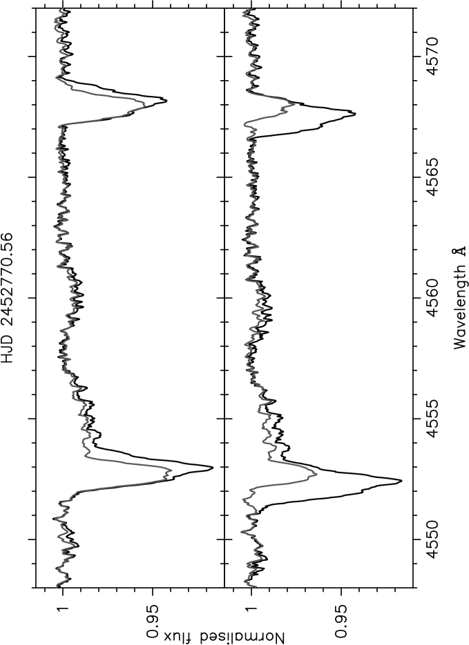
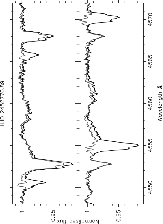
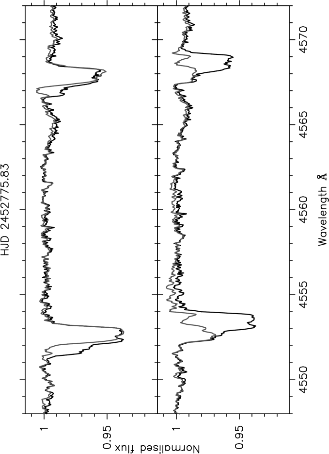
The first part of the time-series of Lup was gathered with the FEROS échelle spectrograph attached to the 2.2m ESO telescope at ESO, La Silla, Chile during the nights of 11–16 May 2003. The night of 15 May was mainly lost due to bad weather. The spectra have a resolution and cover the range 3500 to 9200 Å, divided into 39 orders. We obtained 56 spectra with an average S/N-ratio of 450 in the spectral range of the Si iii triplet near 4568 Å. The integration times were between 5 and 13 minutes. A logbook of the 6 nights is given in the top part of Table 1. The data reduction was performed using the on-line FEROS reduction pipeline, which makes use of the ESO-MIDAS software package. We performed an additional correction for the wavelength sensitivity of the shape of the internal flatfields by means of a smoothed average of dome flatfields. For each of the 6 nights, a randomly chosen set of normalised FEROS spectra centered at the Si iii triplet near 4568 Å is given at the bottom of Fig. 2.

The second part of the time-series of Lup consists of 47 spectra () measured with the GIRAFFE échelle spectrograph at the 1.9m telescope at SAAO, Sutherland, South Africa. From the 7 nights of 20–26 May 2003, 3 nights were lost due to bad weather. Integration times were between 5 and 10 minutes. The total wavelength range covers 4400-6680 Å and is spread over 45 orders. Due to the lower resolution the GIRAFFE data are of lower quality than the FEROS data. The average S/N-ratio we obtained was 200. A logbook of the spectra can be found in the lower part of Table 1. The GIRAFFE spectra were reduced by using the GIRAFFE pipeline reduction program xspec2. At the top of Fig. 2 a sample of reduced and normalised GIRAFFE spectra centered on the wavelength region of the Si iii triplet near 4568 Å are shown.
4 The orbital motion
| Nr. | 3 | 1 | 3 | 1+3 | 5+6 |
|---|---|---|---|---|---|
| Elem. | T70 | fotel | fotel | fotel | fotel |
| (days) | fixed | ||||
| fixed | |||||
| (km s-1) | |||||
| (km s-1) | |||||
| (∘) | |||||
| (A.U.) | |||||
| (A.U.) | |||||
| () | |||||
| () | |||||
| (km s-1) | j=1: | j=3: | j=1: | j=5: | |
| — | — | — | j=3: | j=6: | |
| rmsj (km s-1) | — | j=1: | j=3: | j=1: | j=5: |
| — | — | — | j=3: | j=6: | |
| rms (km s-1) | 3.6 | 8.8 | 7.6 | 8.1 | 2.4 |
| (yrs) | 64 | — | — | — | — |
T70 studied the orbital motion of the triple system Lup from spectra obtained with the Radcliffe telescope during 1964-1970. The orbital elements he derived are listed in the first column of Table 3. Our dataset, consisting of 103 spectra obtained from two different observatories, samples the short orbital period approximately 3 times, whereby 80% of all phases is covered. Our short dataset, in combination with the older data, does not allow investigation of the triple system, due to the extremely poor phase coverage.
4.1 Radial velocities
|
|

|
| Nr. | 1,3-6 | 3-6 | 4,5,6 |
| Elem. | fotel | fotel | korel |
| (days) | fixed | ||
| (days) | fixed | ||
| (km s-1) | |||
| (km s-1) | |||
| (∘) | |||
| (∘/yr) | fixed | ||
| (years) | fixed | ||
| (A.U.) | |||
| (A.U.) | |||
| () | |||
| () | |||
| (km s-1) | — | — | |
| (km s-1) | — | ||
| (km s-1) | — | ||
| (km s-1) | — | ||
| (km s-1) | — | ||
| rms1 (km s-1) | 11.2 | — | — |
| rms3 (km s-1) | 9.8 | 8.2 | — |
| rms4 (km s-1) | 5.8 | 5.3 | — |
| rms5 (km s-1) | 1.9 | 1.8 | — |
| rms6 (km s-1) | 2.2 | 2.2 | — |
| rms (km s-1) | 2.9 | 2.6 | — |
We derived the RV values of each of the two components in two different ways: from the first normalised velocity moment (e.g. Aerts et al. 1992) and by means of the cross-correlation (CC) technique.
To calculate of the of the three lines of the Si iii triplet at 4552.654 Å, 4567.872 Å and 4574.777 Å, we used variable integration boundaries. Values of the RVs of the secondary could only be derived at phases near elongation, when both profiles were separated. One has to keep in mind that the estimates of the RVs of the primary near conjunction are contaminated by the presence of the secondary.
We applied the CC technique to several wavelength regions with well-defined absorption lines for primary and secondary. These regions were centered on the following 6 lines: Si iii 4568 Å, Mg ii 4481 Å, He i 5016 Å, He i 4917 Å, He i 5876 Å, and He i 6678 Å. As templates for the CC, we took the average normalised spectrum of the FEROS and of the GIRAFFE datasets. The position of the line center, measured by means of a Gaussian fit, was used as an estimate of the RV. The CC technique also allowed us to determine the RVs of the secondary when its profiles were semi-detached from those of the primary. Finally, we calculated the median RV of the 6 regions and its standard deviation.
It turned out that the scatter on the first velocity moment calculated from the Si iii profiles of the FEROS spectra was less than for the RVs calculated by CC. This is possibly due to the good quality and high-resolution of the FEROS spectra and the nicely defined absorption profiles of the Si iii triplet. Therefore we used the values of the average of the first moments of the 4553 Å and 4568 Å profiles as RVs of the FEROS time-series in the subsequent analysis. The GIRAFFE spectra, on the other hand, are of lower quality than the FEROS spectra. For these spectra the noise was suppressed by the CC procedure, so that we used the median of the CC measurements as RVs of the GIRAFFE time-series.
Additionally, we included the three high-quality (R65 000, S/N 450) CAT spectra, obtained by Schrijvers et al. (2002) in 1995-1996. We calculated the first normalised velocity moment for both primary and secondary.
We enlarged our sample of RV measurements with the ones T70 used for his analysis. These datapoints include 10 values calculated from spectrographic plates obtained from Lick Southern Station, Chile, between 1907 and 1911, and 32 RVs calculated from several spectral lines measured with the Radcliffe 74-inch reflector at Radcliffe Observatory during 1964–1970. We recalculated more accurate HJD values for the Lick data, based on the information given by Campbell & Moore (1928) and discovered that in their ambiguous notation the RVs of primary and secondary of nights HJD 2417703 and HJD 2418760 were exchanged. For 25 of the 42 datapoints, RVs for both components are given. Also three RV measurements (1955–1956), provided with errors, are available from Buscombe & Morris (1960). A journal of all available RVs we used for the further analysis is given in Table 2, while the individual RVs with corresponding HJDs can be found in Table LABEL:onlinedata111Table LABEL:onlinedata is only available in electronic form.. The error estimates, given in Table LABEL:onlinedata only for our observations, are the rms errors of the mean of Si iii, Mg ii, and He i RVs.
4.2 Determination of the orbital parameters
Analysis of RVs was carried out using the fotel code (Hadrava 1990), which is designed to solve the light- and/or RV curves of binary stars with a possible third component and also can model secular changes in the orbital period and apsidal motion. To each individual RV we assigned a weight which is proportional to the spectral resolution : . The spectral resolution can be expressed by the formula
| (1) |
with the central wavelength of the spectrum in question in Å, its linear dispersion in Å/mm-1, the “pixel” spacing in mm, and the number of d per FWHM of the projected slit width, which has a typical value of 2-3. We adopted the values =0.020 mm and =2 for the photographic spectra. Information on the dispersion or resolution of the different types of data is provided in Table 2.
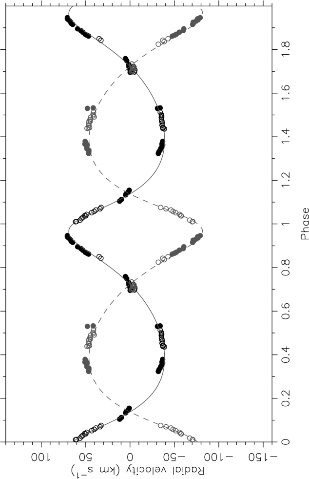
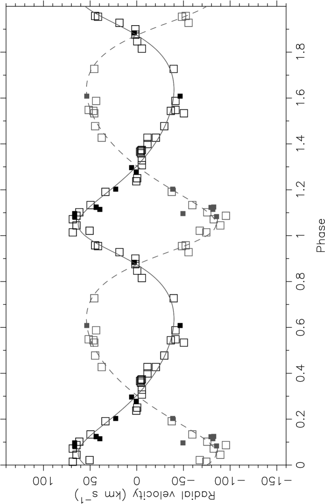
First, we calculated a local solution for the subsets of Radcliffe, Lick, and the combined FEROS and GIRAFFE data. In the case of the Lick data we kept the values of the orbital period and eccentricity fixed. For the new data, measurements with errors larger than 10 km s-1 were rejected. These uncertain measurements correspond to datapoints near conjunctions. The lack of accurate datapoints close to the system velocity due to blending of the lines is a typical problem that occurs for SB2s. One of the consequences is that orbital parameters whose determination is sensitive to the velocity behaviour near conjunction, such as the eccentricity and the periastron longitude , will be less accurately derived. The resulting parameters of the sub-datasets are listed in Table 3. From the old dataset of Lick and Radcliffe measurements we found a solution consistent with the one T70 derived from the Radcliffe data (). The RVs of the FEROS and GIRAFFE time-series could be folded with the same orbital period with a slightly higher eccentricity . We note that the values of differ in the different datasets and hence suspected the presence of an apsidal advance.
Secondly, we searched for solutions in larger subsets, thereby allowing for apsidal advance. We worked iteratively in cases of subsets including datasets 4-6: we determined values of and , which were subsequently kept fixed in the KOREL disentangling process of all FEROS, GIRAFFE, and CAT spectra (see Sect. 4.3). As KOREL allows construction of a precise RV curve for both components, even at phases near conjunction, we subsequently ran the FOTEL code again, replacing the FEROS, GIRAFFE, and CAT measurements by the KOREL RVs to optimise the solution.
We investigated the rate of the rotation of the line of apsides in the subsets including Lick and Radcliffe data (datasets 1 and 3, third column Table 3) and Radcliffe, CAT, FEROS, and GIRAFFE data (datasets 3-6, using korel RVs for datasets 4-6, second column Table 4). The bad phase coverage of the Lick data, in combination with its poor quality, did not allow good definition of , so we did not find a significant apsidal advance in the first subset. Next, we combined all datasets, spanning some 96 years, including the few Mount Stromlo and CAT velocities, and searched for the best matching orbital solution. We did not succeed in including the few RV measurements published by Buscombe & Morris (1960), as they fell completely outside our velocity curve. Therefore we question the correctness of these values. The more so because Buscombe & Kennedy (1962) published an unreliable orbital solution with a nearly circular orbit of 0.9 days. Leaving out the Mount Stromlo measurements led to an orbital period of and /yr, the latter value being slightly smaller than obtained from the datasets 3-6. Including the corresponding korel RVs for CAT, FEROS, and GIRAFFE data led to the ’best’ orbital parameters, i.e. with the lowest rms value, given in the first column of Table 4. We stress, however, that although the solutions are quite stable concerning parameters , , , and , uncertainties surround the values of , and consequently also . In order to gain clarity, additional datasets, strategically chosen in time, are needed.
The phase diagrams of Lick & Radcliffe data (4th column, Table 3), FEROS, & GIRAFFE data (last column, Table 3) and FEROS, GIRAFFE, and CAT data (korel solution, last column, Table 4) with respect to are displayed in Fig. 3.
The system velocities of the newly obtained data differ significantly from the older dataset 3 (see Table 4), which supports the presence of a third body. Given the solution of the close binary system as derived from the whole available dataset, we attempted to converge to a solution of the triple system, but – not surprisingly, given the poor phase coverage – without satisfactory results. To unravel the triple system with an orbital period of approximately 64 years, a dedicated long-term project is required with the aim of gathering datapoints that are well-spread in the orbital phase.
4.3 Spectral disentangling
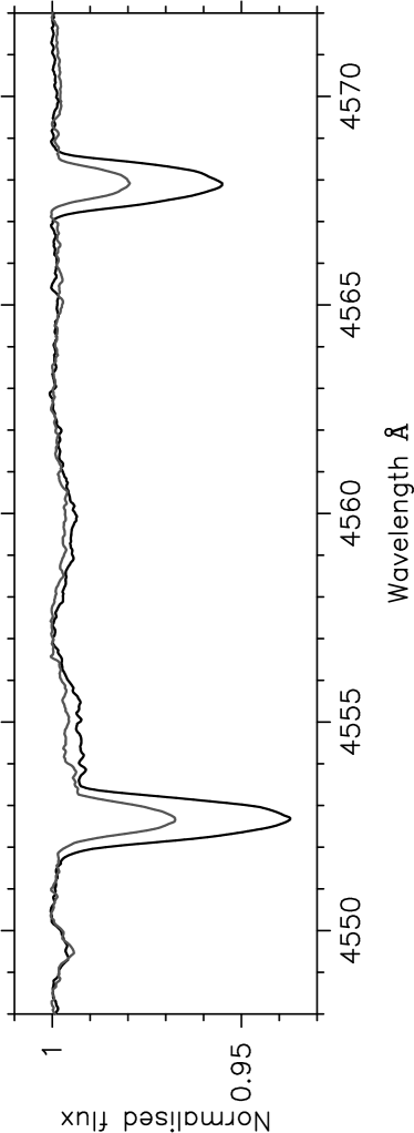
An advantage of the korel code (Hadrava 1995) is that it allows the study of a spectral range as a whole and thereby can extract information from the blended lines. We applied the korel disentangling technique to the set of CAT, FEROS, and GIRAFFE spectra and focussed on the wavelength region centered on the two bluest lines of the Si iii triplet. One spectrum was removed from the dataset due to its poor quality. We included apsidal motion to account for the time gap of 2574 days between the CAT data and the data taken in May 2003. We note, however, that given the small amount of CAT spectra, the solutions allowing for apsidal advance do not differ significantly from the ones not taking apsidal motion into account. We kept the orbital period fixed on its best fotel solution () and searched for the most satisfactory solution of orbital elements in combination with the ’best’ decomposition of the spectra. The resulting elements are listed in the last column of Table 4, and the derived RVs of primary and secondary are plotted versus orbital phase in the lower panel of Fig. 3. The normalised disentangled spectra centered at 4560 Å are given in Fig. 4.
5 Limits on physical elements
5.1 Estimates of basic physical elements
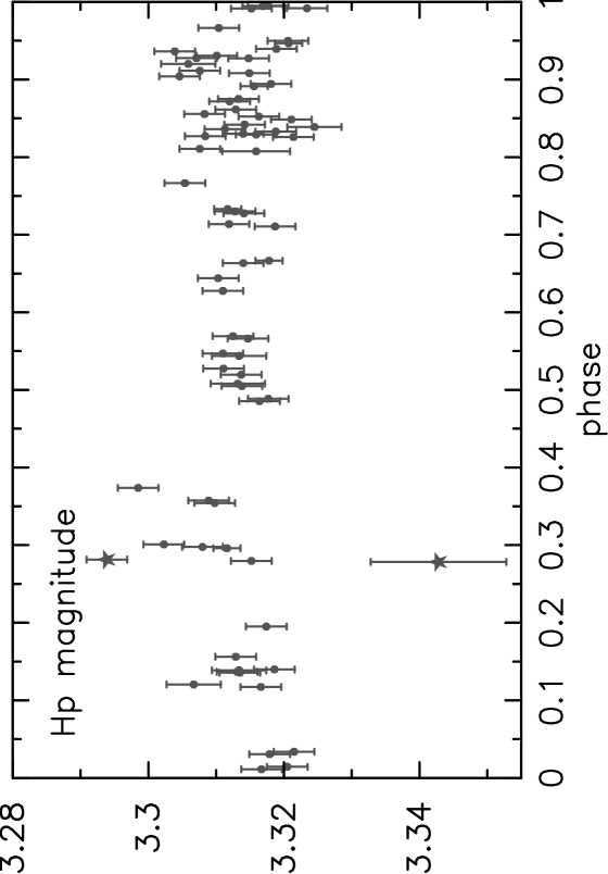
An important unknown in the unravelling of the physical parameters of binary components is the orbital inclination, which can only be accurately determined in case the star is an eclipsing binary. In the literature no evidence for the presence of eclipses in Lup is found. We looked at the HIPPARCOS lightcurve of Lup. The data with quality label 0 are plotted versus orbital phase in Fig. 5. We see that one datapoint shows a decrease in brightness. This happens to be the measurement with by far the largest error bar, which is moreover measured 15 minutes apart from the brighest datapoint in the dataset, spanning more than 1000 days. Therefore we consider this insufficient evidence to claim the presence of an eclipse. Assuming that Lup is a non-eclipsing system implies an orbital inclination lower than 50 degrees (), given the B-type nature of the two components.
We estimated the radius of the primary by using the formula
| (2) |
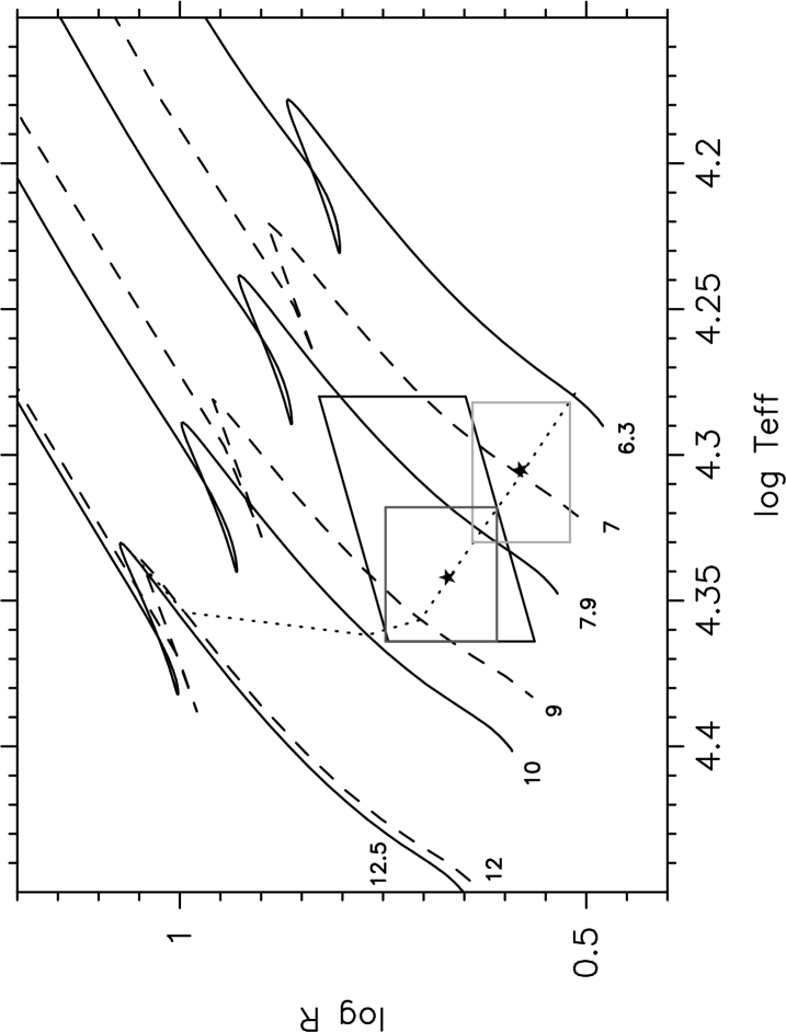
with the HIPPARCOS parallax ( mas, Perryman et al. 1997), the bolometric correction, reddening , effective temperature , and magnitude. From the HIPPARCOS photometry transformed to the Johnson magnitude by using Harmanec’s (1998) transformation formula and from the Geneva photometry, we find = 3375 and = 3369, respectively. The corresponding dereddened value of the latter is 332. Next, we considered two situations: that the two components are equally bright in the magnitude, implying 406, and that the secondary is half as bright as the primary, hence 375. These two situations are realistic limits on the true value of . Considering a range of , which is consistent with a spectral type between B3 and B2 according to Harmanec’s tabulation (1988), formula 2 leads to a radius of the primary between 3.6 and 6.7 (black box in Fig. 6).
By comparing our observations with Schaller’s et al. (1992) and Claret’s (2004) evolutionary models (see Fig. 6), and assuming an age of 15 Myr (dotted line) of the Lup system as a member of the UCL OB association (De Zeeuw et al. 1999), we find the following restrictions on the radius, mass and of the primary of Lup: , and (dark gray box in Fig. 6). Using this range of masses for the primary we can narrow down the interval of the orbital inclination and of the mass of secondary. From the values and , derived from the best fotel solution, we find and . These values of are thus compatible with the lack of observational evidence for eclipses. The evolutionary tracks (see Fig. 6) for a secondary with and the same age as the primary, impose the following limits: and (light gray box in Fig. 6). The physical parameters of representatives of the primary and secondary of Lup, indicated by asterisks in Fig. 6 and given in Table 5, are compatible with a B3IV and B3V star as suggested by T70.
| star | (∘) | () | |||
|---|---|---|---|---|---|
| 1 | 4.34 | 4.7 | 8.7 | 20.5 | 29.2 |
| 2 | 4.31 | 3.8 | 7.3 |
From the Full Width Half Intensity (FWHI) of the disentangled profiles (Fig. 4), we measured projected rotational velocities according to the formula , and arrive at values km s-1 and km s-1 for the primary and secondary, respectively. These values are compatible with the value of 40 km s-1 Slettebak et al. (1975) listed in their catalogue. Assuming leads to the following limits on the equatorial rotational velocities: km s-1 and km s-1. For a primary and secondary with radii as derived above, we estimate a rotational period between and days ( c d-1), respectively, and days ( c d-1). Given all uncertainties involved, it is quite possible that both components have identical rotational periods, possibly corresponding to the spin-orbit synchronization at periastron, observed for many eccentric-orbit binaries. For Lup its value is 481 if the eccentricity from the KOREL solution is adopted (cf. formula 7 and relevant discussion in Harmanec 1988).
We have to bear in mind that, due to several limitations on our dataset, the derived values of , , () and the orbital inclination are only rough estimates, derived under certain assumptions. Additional information from future interferometric observations would provide a much more accurate determination of the component masses and radii, as well as the orbital inclination and the relative luminosities of the components.
5.2 Interpretation of the observed apsidal motion
The range of apsidal periods we derived in Sect. 4.1 () is consistent with the values obtained for other binaries with orbital periods between 4 and 5 days (Petrova & Orlov 1999). As a comparison, we mention the system QX Car, which is very similar to Lup, and consists of two B2V stars orbiting in an eccentric () orbit of 4.5 days, which has an apsidal period of 370 years.
The
tide-generating potential of the binary system can give rise to a periodic variation of the longitude of periastron. It is well-known that the observed apsidal advance in eccentric-orbit
binaries arises from both classical and general-relativistic
terms, i.e.
.
We calculated the contribution of the relativistic term from the formula
given by Giménez (1985),
which resulted in yr and which is a 6-7 times smaller value than our observed range of values.
An estimate of the total contribution of classical effects can be derived from and leads to yr. The classical effects are caused by tidal and rotational distortions, and, if relevant, the presence of a third body: . The latter term is negligible in the case of Lup due to the long orbital period of the triple system. According to the formula given by Wolf et al. (1999), the contribution of the third component to the rotation of the line of apses is estimated as . Neglecting this effect, we estimated a mean apsidal constant (cf. formula 4 in Claret & Willems 2002) for the primary and secondary from the observed apsidal period and relative photometric radii of the components, and , as for the representative set of values from Table 5. This can be compared with the theoretically expected values, interpolated from Claret’s (2004) models, and for the primary and secondary, respectively. It is seen that there is no obvious conflict between the observed and theoretically predicted values. Given our observed range of primary radii, assuming , and , we estimate the rate of secular apsidal motion due to the tidal distortion of the components from the formula given by Claret & Willems (2002, their formula 13): yr yr. As we could derive only rough estimates of the basic physical properties of both stars, we do not take into account the possible effect of dynamic tides studied by Claret & Willems (2002). We note, however, that their effect will probably be small as the stars are rotating close to spin-orbit synchronization at periastron unless there is some resonance present in the system. This must be left unanswered until much more accurate masses and radii of components are known. The estimated values of and lead us to conclude that the term , accounting for rotational effects, must contribute significantly to the apsidal motion.
6 Intrinsic variability
|
|
|
| HJD 2452771 | HJD 2452773 |
|
|
|
|
High-degree () modes are suspected in the primary of Lup (Schrijvers et al. 2002; Fig. 1). The analysis of LPVs of both primary and secondary is a challenging task due to the comparable line-strength of the two components and the blending of the component lines in phases far from elongation. The spectra of two line-profile variable components that have been disentangled by korel have never been the subject of an LPV study before. We investigate the two bluest Si iii profiles before and after korel disentangling and then compare the results. A disadvantage of using the original spectra is that only spectra obtained at phases of elongation can be used, while all korel disentangled profiles can be considered for analysis. However we question whether the intrinsic variations of primary and secondary are properly disentangled, as korel is not constructed to treat pulsational variations. For the testcase Sco, Harmanec et al. (2004) and Uytterhoeven et al. (2005) obtained good results concerning the retrieval of intrinsic variations with high amplitude after disentangling but the performance of korel was less clear for low amplitude variations.
The set of disentangled profiles of the first (second) component were constructed by adding the korel residuals calculated in the restframe of the primary (secondary) to the normalised disentangled profile of the primary (secondary). The ’original profiles’ of the first (second) component were obtained from the observed spectra by a shift in wavelength according to its corresponding orbital velocity in the best-fitting orbit obtained with korel (last column in Table 4, bottom panel in Fig. 3). In Fig. 7 we compare the original and disentangled profiles of the primary and the secondary at three different orbital phases. From these comparison plots we conclude the following: 1. The primary and secondary of Lup are line-profile variables. 2. The korel residuals in the restframe of the primary (secondary) contain signatures of the intrinsic variability of both components.
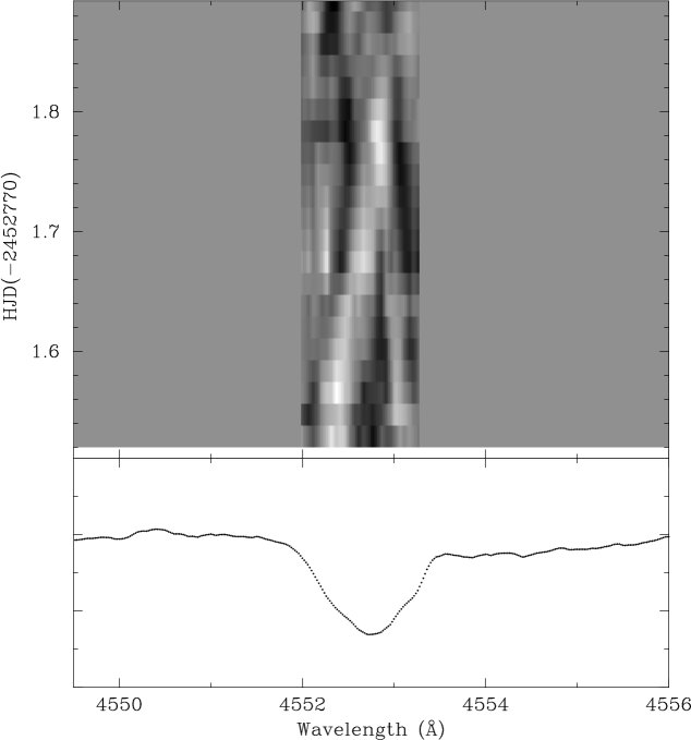
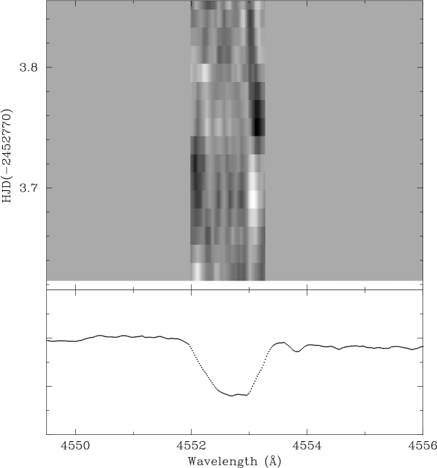
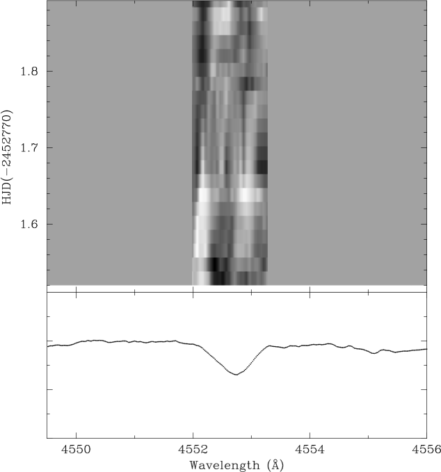
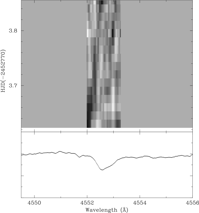
In order look closely for signs of intrinsic variability, we show the grayscale representations of the disentangled Si iii 4553 Å profiles of the primary and secondary on two nights during the FEROS observing run when the two components are near elongation (Fig. 8). To bring out the variability of the primary and secondary in full detail, we calculated the residuals with respect to the nightly average spectrum. For both components we find signatures of intrinsic variability, although weak in case of the secondary, in the form of moving black and white bands.

|

|
We performed clean (Roberts et al. 1987), Lomb-Scargle (Scargle 1982) and Phase Dispersion Minimisation (PDM, Stellingwerf 1978) analyses on the first three velocity moments (), the EW, and the RVs associated to the minimum of each line-profile, in search for intrinsic variations of primary and secondary. Also the 2D-analysis Intensity Period Search (IPS, Telting & Schrijvers 1997), to find variable signals in individual wavelength bins ( Å in case of Lup), was performed by using the CLEAN algorithm. All the diagnostics were calculated from the Si iii 4552.654 Å and 4567.872 Å profiles of both the disentangled and original profiles.
We investigated the variable signal of the complete datasets, including all datapoints, and of reduced datasets, which included only the 56 datapoints obtained when the lines of the component spectra were separate (for a logbook, see Table 1). The clearest signals were detected in the variability of the latter datasets for the obvious reason that unreliable datapoints near conjunction were not included. In theory, all datapoints after disentangling should contain reliable information about the variability of the primary (secondary), but the observations show that even for the disentangled profiles, this restriction to the 56 separate spectra is to be preferred. For the moment it is unclear how well the korel disentangling procedure can separate the intrinsic variability contributions of the primary and secondary near conjunction. This can only be deduced from a dedicated simulation study, which is beyond the scope of the current work.
Below, we report on the results obtained from the reduced datasets
containing 56 datapoints and spanning 12 days. The window
function is very complicated and leads to severe aliasing. The half width at half maximum of the amplitude of the highest window
peak is as large as 0.03 c d-1 and gives a rough estimate of
the error on the frequencies. According to the empirically derived
formula by Cuypers (1987), the small dataset allows a frequency accuracy of 0.01 c d-1. Hence, we searched for frequencies in the frequency domain between 0 and 20 c d-1, with frequency steps of 0.01 c d-1.
A more extended discussion of the frequency analysis results than presented here can be found in Uytterhoeven (2004)222PhD thesis available from
http://www.ster.kuleuven.be/pub/uytterhoeven_phd/.
6.1 Intrinsic variability of the primary
No clear dominant frequency is found in the variability of the primary. The highest amplitude is found between 0-2 c d-1. In the Scargle periodogram of the non-prewhitened data, as shown in the upper panel of Fig. 9, one sees hints of the presence of a variability near 6.46 c d-1 or one of its aliases, but these peaks reduced in amplitude (original profiles) or almost completely vanished (disentangled profiles) after prewhitening with the highest amplitude low frequency peak (lower panel of Fig. 9). Signatures of the peak 6.46 c d-1 are also found at very low amplitude in the IPS analysis.
The EW of the primary’s original profiles shows variations with frequency 0.83 c d-1. This value is also recovered in the second moment and in the IPS analysis, and can be related to 0.44 c d-1, detected in the EW variations of the disentangled spectra, through a peak of the window function. As stellar rotational frequencies are not uncommonly detected in the EW of line profiles (e.g. Sco, Uytterhoeven et al. 2005; V2052 Oph, Neiner et al. 2003; Cephei , Telting et al. 1997), we might consider this frequency to be related to the rotation of the star. Indeed, the value 0.44 c d-1 is compatible with the rotational period assuming spin-orbit synchronization, as derived in Sect. 5.
6.2 Intrinsic variability of the secondary

|

|
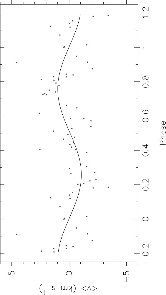
The line profiles of the secondary of Lup show variations with a frequency near 10.36 c d-1 (hereafter called ) and with a velocity amplitude of km s-1. This frequency, or an alias, appears in all diagnostics after prewhitening with 0.39 c d-1 or one of its aliases (Fig. 10). A phase diagram of the first velocity moment of the disentangled profiles folded with 10.36 c d-1, is given in Fig. 11. The frequency 10.36 c d-1 is not recovered from the IPS analysis. The EW of the secondary’s original profiles varies with 0.75 c d-1, or one of its aliases.
We note that the frequency 0.05 c d-1, detected in the IPS analysis of the profiles of the secondary, also appears in the IPS analysis performed on the profiles of the primary. This frequency is most probably a reflection of the orbital motion in the profiles, given the following relation within the frequency resolution: . Similar relations between intrinsic frequencies and the orbital frequency are observed in other close binary stars (e.g. Vir, , Smith 1985; Sco, , Chapellier & Valtier 1992).
The period of about 2 hours is relatively short for Cephei type pulsations. A few examples of Cephei stars with similar frequency values are known (for an overview see Aerts & De Cat 2003). So far, the highest frequency reported in the literature amounts to 15 c d-1 and corresponds to a very low RV amplitude ( Sco, Telting & Schrijvers 1998). The low-amplitude frequency we found in the secondary of Lup resembles the low-amplitude frequencies c d-1 and c d-1 detected in the B-type primary of the spectroscopic binary Orionis (Telting et al. 2001), which were interpreted in terms of high-degree pulsation modes. To confirm the presence of and refine its value, additional monitoring of Lup is required. As the intrinsic variability of the secondary can only be studied at orbital phases near elongation, one should aim to gather data during these phases.
Frequency shows up in both original and disentangled datasets. This result indicates that the variability inherent to the secondary is well preserved through korel disentangling during orbital phases near elongation.
7 Summary and discussion
From a dataset of 106 high-resolution spectra obtained quasi-consecutively from two different observatories with a time-span of 20 days, we were able to refine the orbital parameters of the close orbit of the triple system Lup by using the fotel and korel codes. As the star is an SB2, we obtained RVs for both components and found an eccentric () orbit of days. By adding our data to published RV measurements we found strong evidence of the presence of apsidal motion ( years). In order to solve the triple system, as well as to further investigate the effect of apsidal motion, an extensive dataset, spanning several decades, is required.
Two stars of spectral type between B3 and B2 in the close orbit, as suggested before by T70, agree with our orbital solution. We estimated the component masses and . Both components may be spin-orbit synchronized. Interferometric measurements would be a mayor step foreward in accurately determining the physical parameters of the system. The triple system Lup is a very suitable target for large interferometers.
We used the korel disentangling technique as an intermediate step in the study of the two early-B type line-profile variable stars of similar brightness. The variability of primary and secondary seems to be preserved well after disentangling.
Although the grayscale representations clearly show signs of the presence of variability, we were not able to detect a dominant frequency in the line profiles of the primary. We thus classify the first component of Lup as a Cephei suspect. On the other hand, a candidate pulsational frequency was found in the variability of the secondary, near 10.36 c d-1. Its precise value could not be determined due to the poor frequency resolution. This frequency certainly needs confirmation by means of additional intensive monitoring. Nevertheless, we propose the secondary of Lup as a new Cephei variable.
Further investigation of the intrinsic variability of both components of Lup requires a follow-up multi-site campaign with intensive monitoring of the star, preferably at phases near elongation, by means of high-resolution spectroscopy. For an example of the benefit of such a multi-site campaign, we refer to Handler et al. (2004) and Aerts et al. (2004b).
The detection of several observational cases of tidally induced oscillations is necessary to improve our understanding of the relation between tidal interaction and the excitation of pulsation modes, and the seismic modelling of such stars. Effects such as the deformation of the spherical shape of a star due to tidal forces are usually not taken into account in theoretical calculations. Aerts et al. (2002) have shown that, in the case of the Scuti star XX Pyx, deformation of the star due to the tide-generating potential is clearly more important for interpreting the pulsational behaviour than is the rotational deformation. The tide-generating potential is proportional to , while the deformation due to centrifugal forces is proportional to . The values derived by Aerts et al. (2002) for XX Pyx were and . We also calculated the contributions of the tidal forces and rotation on the deviation of spherical symmetry for the secondary of Lup. Assuming , (Table 5) and assuming spin-orbit synchronization c d-1, we derived and ; hence, is larger than . As a comparison we calculated and for the hybrid Doradus star HD 209 295 for which tidally induced oscillations indeed have been detected (Handler et al. 2002). As not all parameters are given by these authors, we can only give a rough estimate: the value of is on the order of , while is 3 orders of magnitude larger. For this system, the rotational effects on the oscillations are thus larger than the tidal effects. These examples show that variety of behaviour exists amongst close binary systems. Only confrontation between several observational findings and theory can bring us closer to understanding the mutual interaction between the mechanisms that play a role in the properties of oscillations in close binary systems.
Acknowledgements.
The authors acknowledge Dr. P. Hadrava for sharing his codes korel and fotel . This study has benefited greatly from the senior fellowship awarded to PH by the Research Council of the University of Leuven, which allowed his three-month stay at this university. KU is supported by the Fund for Scientific Research – Flanders (FWO) under project G.0178.02 and CA by the Research Fund K.U.Leuven under grant GOA/2003/04.References
- (1) Aerts, C., & Harmanec, P. 2004, in Spectroscopically and Spatially Resolving the Components of Close Binary Stars, ASP Conf. Ser. 318, 325
- (2) Aerts, C., De Pauw, M., & Waelkens, C. 1992, A&A, 266, 294
- (3) Aerts, C., De Mey, K., De Cat, P., et al. 1998, in A Half century of Stellar Pulsation Interpretation, ed. P.A. Bradley & J.A. Guzik, ASP Conf. Ser. 135, 380
- (4) Aerts, C., Handler, G, Arentoft, T., et al. 2002, MNRAS, 333, L35
- (5) Aerts, C., & De Cat, P. 2003, SSR, 105, 453
- (6) Aerts, C., De Cat, P., Handler, G., et al. 2004, MNRAS, 347, 463
- (7) Bernacca, P.L., & Perinotto, M. 1970, CoAsi. 239, 1
- (8) Buscombe, W., & Kennedy, P.M. 1962, PASP, 74, 323
- (9) Buscombe, W., & Morris, P.M. 1960, MNRAS, 121, 263
- (10) Campbell, W.W., & Moore, J.H. 1928, Publ. Lick Obs., 16, 223
- (11) Castelli, F. 1991, A&A, 251, 106
- (12) Chapellier, E., & Valtier, J.C. 1992, A&A, 257, 587
- (13) Claret, A. 2004, A&A, 424, 919
- (14) Claret, A., & Willems, B. 2002, A&A, 388, 518
- (15) Curtis, H.D. 1909, Lick Obs. Bull., 5, 139
- (16) Cuypers, J. 1987, The Period Analysis of Variable Stars, Academiae Analecta, Royal Academy of Sciences 49 - 3, Belgium
- (17) De Cat, P. 2002, in Radial and Nonradial Pulsations as Probes of Stellar Physics, ed. C. Aerts, T.R. Bedding & J. Christensen-Dalsgaard, ASP Conf. Ser. 259, 196
- (18) De Cat, P., & Aerts, C. 2002, A&A, 393, 956
- (19) de Vaucouleurs, A. 1957, MNRAS, 117, 449
- (20) De Zeeuw, P.T., Hoogerwerf, R., de Bruijne, J.H.J., et al. 1999, AJ, 117, 354
- (21) Giménez, A. 1985, ApJ, 297, 405
- (22) Hadrava, P. 1990, Contr. Astron. Obs. Skal. Pl., 20, 23
- (23) Hadrava, P. 1995, A&AS, 114, 393
- (24) Hadrava, P. 1997, A&ASS, 122, 581
- (25) Handler, G., Balona, L.A., Shobbrook, et al. 2002, MNRAS, 333, 262
- (26) Handler, G., Shobbrook, R. R., Jerzykiewicz, M., et al. 2004, MNRAS, 347, 454
- (27) Harmanec, P. 1988, BAIC 39, 329
- (28) Harmanec, P. 1998, A&A, 335, 173
- (29) Harmanec, P., Hadrava, P., Yang, S., et al. 1997, A&A, 319, 867
- (30) Harmanec, P., Uytterhoeven, K., & Aerts, C. 2004, A&A, 422, 1013
- (31) Hiltner, W.A., Garrison, R.F., & Schild, R.E. 1969, ApJ, 157, 313
- (32) Hoffleit, D. 1991, The Bright Star Catalogue, 5th revised edition, Yale University Observatory, New Haven, Connecticut, USA
- (33) Levato, H., &Malaroda, S. 1970, PASP, 82, 741
- (34) Moore, J.H. 1910, Lick Obs. Bull., 6, 151
- (35) Morossi, C., & Malagnini, M.L. 1985, A&AS, 60, 365
- (36) Neiner, C., Henrichs, H.F., Floquet, M., et al. 2003, A&A, 411, 565
- (37) Pamyatnykh, A.A. 1999, Acta Astr., 49, 119
- (38) Perryman, M.A.C., Lindegren, L., Kovalevsky, J., et al. 1997, A&A, 323, L49
- (39) Petrova, A.V., & Orlov, V.V. 1999, AJ, 117, 587
- (40) Roberts, D. H., Lehar, J., & Dreher, J. W. 1987, AJ, 93, 968
- (41) Scargle, J. D. 1982, ApJ, 263, 835
- (42) Schaller, G., Schaerer, D., Meynet, G. et al. 1992, A&AS, 96, 269
- (43) Schrijvers, C., Telting, J.H., & De Ridder, J. 2002, in Radial and Nonradial Pulsations as Probes of Stellar Physics, ed. C. Aerts, T.R. Bedding & J. Christensen-Dalsgaard, ASP Conf. Ser. 259, 204
- (44) Slettebak, A. Collins G.W., Boyce, P.B., et al. 1975, ApJS, 281, 29
- (45) Smith, M.A. 1985, ApJ, 297, 224
- (46) Sokolov, N.A. 1995, A&ASS, 110, 553
- (47) Stellingwerf, R.F. 1978, ApJ, 224, 953
- (48) Telting, J.H., & Schrijvers, C. 1997, A&A, 317, 723
- (49) Telting, J.H., Aerts, C., & Mathias, P. 1997, A&A, 322, 493
- (50) Telting, J.H., & Schrijvers, C. 1998, A&AS, 339, 150
- (51) Telting, J.H., Abbott, J.B., & Schrijvers, C. 2001, A&A, 377, 104
- (52) Telting, J.H., Uytterhoeven, K., & Ilyin, I. 2003, in Asteroseismology across the HR diagram, ed. Thompson M.J., Cunha M.S. & Monteiro M.J.P.F.G, Ap&SS, 284, 401 (CDrom)
- (53) Thackeray, A.D. 1970, MNRAS, 149, 75 (T70)
- (54) Tokovinin, A.A. 1997, A&ASS, 174, 75
- (55) Uesugi, A., & Fukuda, I. 1970, CoKwa., 189
- (56) Uytterhoeven, K. 2004, Ph.D. Thesis, KULeuven, Belgium
- (57) Uytterhoeven, K., Briquet, M., Aerts, C., et al. 2005, A&A, 432, 955
- (58) Wolf, M, Diethelm, R., & Šarounová, L. 1999, A&A, 345, 553
| Date (HJD) | RV1 | error1 | RV2 | error2 | Note |
|---|---|---|---|---|---|
| 2417691.7678 | -37.6 | 62.5 | A | ||
| 2417703.5991 | 31.2 | -30.0 | A | ||
| 2418760.9114 | 74.9 | -77.3 | A | ||
| 2418825.7282 | 14.2 | A | |||
| 2418829.4971 | 52.3 | -70.6 | A | ||
| 2419112.9000 | 9.2 | A | |||
| 2419156.7000 | 11.3 | A | |||
| 2419157.6720 | 74.8 | -41.5 | A | ||
| 2419157.8070 | 52.5 | -74.2 | A | ||
| 2419221.5900 | 47.6 | -73.4 | A | ||
| 2435297.9640 | 28.0 | -9.0 | B | ||
| 2436793.8760 | 4.0 | -19.0 | B | ||
| 2436798.8560 | 8.0 | -21.0 | B | ||
| 2438456.5951 | -42.0 | 54.0 | C | ||
| 2438463.6087 | 77.0 | -74.0 | C | ||
| 2438478.6309 | 5.0 | C | |||
| 2438481.5881 | 77.0 | -66.0 | C | ||
| 2438494.5070 | 8.0 | C | |||
| 2438505.4036 | 9.0 | C | |||
| 2438518.4670 | 70.0 | -67.0 | C | ||
| 2438520.4831 | -28.0 | 55.0 | C | ||
| 2438563.4078 | 53.0 | -44.0 | C | ||
| 2438588.3454 | -12.0 | 46.0 | C | ||
| 2438595.3089 | 50.0 | -40.0 | C | ||
| 2438598.1947 | -33.0 | 52.0 | C | ||
| 2438599.2336 | 3.0 | C | |||
| 2438600.2796 | 73.0 | -81.0 | C | ||
| 2438601.2175 | 8.0 | C | |||
| 2438602.2524 | -21.0 | 53.0 | C | ||
| 2438604.1792 | 10.0 | C | |||
| 2438884.4871 | 3.0 | C | |||
| 2438906.4533 | 42.0 | -29.0 | C | ||
| 2439363.1908 | 4.0 | C | |||
| 2439363.2438 | 4.0 | C | |||
| 2439625.4602 | 10.0 | C | |||
| 2439626.4213 | 73.0 | -87.0 | C | ||
| 2439671.2942 | 27.0 | -47.0 | C | ||
| 2439696.2405 | -3.0 | C | |||
| 2439696.3665 | -3.0 | C | |||
| 2439723.1773 | 3.0 | C | |||
| 2439723.2742 | 3.0 | C | |||
| 2439756.1914 | -33.0 | 60.0 | C | ||
| 2440012.3611 | -31.0 | 54.0 | C | ||
| 2440333.3966 | 58.0 | -51.0 | C | ||
| 2440369.3663 | 59.0 | -59.0 | C | ||
| 2449965.6037 | -38.4 | 2.0 | 47.7 | 4.5 | D |
| 2450195.8947 | 76.0 | 2.1 | -66.1 | 5.5 | D |
| 2450196.6035 | 13.0 | 3.5 | 13.7 | 6.5 | D |
| 2452770.5066 | -1.3 | 8.2 | D | ||
| 2452770.5109 | -2.9 | 7.7 | D | ||
| 2452770.5170 | -2.0 | 7.6 | D | ||
| 2452770.5368 | -1.9 | 7.3 | D | ||
| 2452770.5587 | -2.4 | 6.8 | D | ||
| 2452770.6025 | -1.6 | 6.2 | D | ||
| 2452770.6388 | -1.1 | 4.4 | D | ||
| 2452770.6604 | -0.3 | 4.2 | D | ||
| 2452770.6930 | -1.5 | 4.2 | D | ||
| 2452770.7516 | -0.1 | 4.6 | D | ||
| 2452770.7702 | -0.9 | 2.2 | D | ||
| 2452770.7896 | -1.2 | 2.3 | D | ||
| 2452770.8095 | 0.0 | 2.4 | D | ||
| 2452770.8296 | 0.3 | 2.6 | D | ||
| 2452770.8493 | 0.7 | 2.7 | D | ||
| 2452770.8704 | 1.3 | 2.7 | D | ||
| 2452770.8899 | 0.5 | 3.3 | D | ||
| 2452770.9119 | 1.5 | 2.8 | D | ||
| 2452771.5107 | 46.7 | 4.8 | -47.7 | 5.7 | D |
| 2452771.5300 | 48.7 | 4.7 | -50.3 | 7.5 | D |
| 2452771.5491 | 50.5 | 5.5 | -52.2 | 8.6 | D |
| 2452771.5918 | 53.3 | 5.2 | -55.6 | 11.3 | D |
| 2452771.6262 | 55.4 | 5.2 | -59.9 | 17.4 | D |
| 2452771.6631 | 59.0 | 4.6 | -60.6 | 7.8 | D |
| 2452771.7543 | 64.6 | 6.7 | -70.6 | 11.6 | D |
| 2452771.7782 | 66.3 | 2.0 | -71.5 | 12.4 | D |
| 2452771.8008 | 66.8 | 3.3 | -71.2 | 7.1 | D |
| 2452771.8251 | 67.8 | 3.5 | -74.5 | 7.8 | D |
| 2452771.8491 | 69.2 | 3.7 | -76.6 | 11.7 | D |
| 2452771.8720 | 70.6 | 4.5 | -76.1 | 13.0 | D |
| 2452771.8961 | 70.5 | 2.8 | -79.0 | 13.3 | D |
| 2452772.6170 | 11.7 | 5.5 | D | ||
| 2452772.6505 | 9.8 | 3.4 | D | ||
| 2452772.7490 | 5.0 | 3.8 | D | ||
| 2452772.7740 | 4.3 | 3.7 | D | ||
| 2452772.8111 | 2.1 | 6.4 | D | ||
| 2452772.8455 | 0.9 | 5.4 | D | ||
| 2452773.6156 | -31.9 | 4.8 | 46.6 | 9.1 | D |
| 2452773.6476 | -32.5 | 4.8 | 46.4 | 9.1 | D |
| 2452773.6813 | -33.8 | 4.6 | 46.3 | 9.6 | D |
| 2452773.7155 | -34.6 | 3.2 | 48.7 | 9.6 | D |
| 2452773.7450 | -35.7 | 3.1 | 48.7 | 9.3 | D |
| 2452773.7722 | -36.2 | 3.2 | 48.6 | 9.1 | D |
| 2452773.7945 | -36.8 | 3.3 | 48.3 | 7.4 | D |
| 2452773.8105 | -36.0 | 4.3 | 50.9 | 7.2 | D |
| 2452773.8389 | -36.5 | 4.5 | 49.8 | 7.4 | D |
| 2452773.8674 | -36.7 | 4.7 | 50.6 | 11.3 | D |
| 2452774.5575 | -30.9 | 4.1 | 48.0 | 14.7 | D |
| 2452774.5683 | -33.9 | 2.1 | 41.5 | 8.4 | D |
| 2452775.5329 | 3.6 | 3.8 | D | ||
| 2452775.5555 | 3.7 | 3.7 | D | ||
| 2452775.5991 | 5.2 | 3.8 | D | ||
| 2452775.7024 | 6.9 | 2.6 | D | ||
| 2452775.7524 | 8.3 | 4.9 | D | ||
| 2452775.8086 | 10.2 | 13.4 | D | ||
| 2452775.8306 | 11.5 | 15.2 | D | ||
| 2452775.8556 | 11.8 | 15.8 | D | ||
| 2452780.2814 | 1.5 | 5.7 | E | ||
| 2452780.3087 | 1.8 | 14.9 | E | ||
| 2452780.3416 | 2.2 | 5.5 | E | ||
| 2452780.3824 | 5.6 | 8.8 | E | ||
| 2452780.5423 | 32.8 | 7.1 | -36.8 | 14.4 | E |
| 2452780.5751 | 34.8 | 8.6 | -42.9 | 5.7 | E |
| 2452781.3053 | 61.3 | 5.8 | -70.3 | 11.0 | E |
| 2452781.3111 | 60.4 | 2.2 | -70.6 | 5.9 | E |
| 2452781.3397 | 56.3 | 5.2 | -67.3 | 13.3 | E |
| 2452781.3733 | 54.7 | 5.3 | E | ||
| 2452781.3930 | 53.4 | 6.0 | E | ||
| 2452781.4285 | 50.0 | 7.9 | -57.7 | 8.9 | E |
| 2452781.4345 | 51.1 | 4.5 | -57.2 | 8.2 | E |
| 2452781.4598 | 48.8 | 4.6 | -55.8 | 7.3 | E |
| 2452781.4953 | 43.2 | 4.6 | -51.5 | 4.9 | E |
| 2452781.5226 | 40.4 | 5.1 | -48.5 | 3.0 | E |
| 2452781.5506 | 38.5 | 3.4 | -46.1 | 4.1 | E |
| 2452781.5776 | 33.8 | 4.3 | -40.5 | 8.9 | E |
| 2452781.6056 | 32.6 | 4.0 | -34.5 | 12.1 | E |
| 2452783.2466 | -38.7 | 4.8 | E | ||
| 2452783.2527 | -38.7 | 4.6 | E | ||
| 2452783.2601 | -36.9 | 3.7 | 48.4 | 13.8 | E |
| 2452783.2666 | -37.3 | 3.6 | 46.9 | 10.6 | E |
| 2452783.2745 | -36.8 | 2.7 | 45.7 | 8.9 | E |
| 2452783.2815 | -36.9 | 2.6 | 45.7 | 9.3 | E |
| 2452783.3250 | -36.1 | 3.2 | 46.4 | 3.9 | E |
| 2452783.3745 | -36.3 | 2.9 | 46.6 | 11.2 | E |
| 2452783.4047 | -35.6 | 3.2 | 46.2 | 4.8 | E |
| 2452783.4123 | -35.9 | 3.0 | 44.7 | 6.5 | E |
| 2452783.4423 | -35.4 | 1.3 | 45.1 | 7.3 | E |
| 2452783.4911 | -35.2 | 1.8 | 44.5 | 7.1 | E |
| 2452783.4974 | -35.6 | 2.4 | 40.4 | 5.9 | E |
| 2452783.5244 | -35.6 | 1.8 | 41.2 | 6.2 | E |
| 2452783.5491 | -35.3 | 1.2 | 41.7 | 7.0 | E |
| 2452783.5988 | -34.0 | 6.0 | 41.1 | 13.9 | E |
| 2452784.2934 | -5.7 | 5.4 | -6.8 | 8.4 | E |
| 2452784.3026 | -5.3 | 4.7 | -6.4 | 8.2 | E |
| 2452784.4391 | -5.0 | 5.4 | -2.1 | 4.1 | E |
| 2452784.4463 | -4.8 | 4.9 | -1.5 | 3.3 | E |
| 2452784.4661 | -0.6 | 4.2 | -2.6 | 4.3 | E |
| 2452784.4708 | -2.2 | 5.1 | -2.4 | 4.5 | E |
| 2452784.4787 | -5.5 | 5.4 | -3.2 | 3.7 | E |
| 2452784.5072 | -4.5 | 4.7 | -4.2 | 5.0 | E |
| 2452784.5116 | -4.5 | 4.9 | -3.0 | 4.6 | E |
| 2452784.5481 | -4.3 | 5.1 | -2.7 | 5.5 | E |
| 2452784.5542 | -2.4 | 3.5 | -2.6 | 4.7 | E |
| 2452784.6059 | -1.9 | 4.1 | -1.8 | 5.1 | E |
| A: Campbell & Moore (1928); B: Buscombe & Morris (1960); C: Thackeray (1970); | |||||
| D: Average of the first moments of the Si iii 4553 Å and 4568 Å profiles; | |||||
| E: Median of the cross-correlation measurements calculated from the Si iii 4568 Å, | |||||
| Mg ii 4481 Å, He i 5016 Å, He i 4917 Å, He i 5876 Å and He i 6678 Å profiles | |||||