MACHOs in M31? Absence of evidence but not evidence of absence

We present results of a microlensing survey toward the Andromeda Galaxy (M31) carried out during four observing seasons at the Isaac Newton Telescope (INT). This survey is part of the larger microlensing survey toward M31 performed by the Microlensing Exploration of the Galaxy and Andromeda (MEGA) collaboration. Using a fully automated search algorithm, we identify 14 candidate microlensing events, three of which are reported here for the first time. Observations obtained at the Mayall telescope are combined with the INT data to produce composite lightcurves for these candidates. The results from the survey are compared with theoretical predictions for the number and distribution of events. These predictions are based on a Monte Carlo calculation of the detection efficiency and disk-bulge-halo models for M31. The models provide the full phase-space distribution functions (DFs) for the lens and source populations and are motivated by dynamical and observational considerations. They include differential extinction and span a wide range of parameter space characterised primarily by the mass-to-light ratios for the disk and bulge. For most models, the observed event rate is consistent with the rate predicted for self-lensing — a MACHO halo fraction of 30% or higher can be ruled at the 95% confidence level. The event distribution does show a large near-far asymmetry hinting at a halo contribution to the microlensing signal. Two candidate events are located at particularly large projected radii on the far side of the disk. These events are difficult to explain by self lensing and only somewhat easier to explain by MACHO lensing. A possibility is that one of these is due to a lens in a giant stellar stream.

1 Introduction

Compact objects that emit little or no radiation form a class of plausible candidates for the composition of dark matter halos. Examples include black holes, brown dwarfs, and stellar remnants such as white dwarfs and neutron stars. These objects, collectively known as Massive Astrophysical Compact Halo Objects or MACHOs, can be detected indirectly through gravitational microlensing wherein light from a background star is amplified by the space-time curvature associated with the object (Paczyński, 1986).

The first microlensing surveys were performed by the MACHO (Alcock et al., 2000) and EROS (Lasserre et al., 2000; Afonso et al., 2003) collaborations and probed the Milky Way halo by monitoring stars in the Large and Small Magellanic Clouds. While both collaborations detected microlensing events they reached different conclusions. The MACHO collaboration reported results that favour a MACHO halo fraction of 20%. On the other hand, the results from EROS are consistent with no MACHOs and imply an upper bound of 20% on the MACHO halo fraction. The two surveys are not inconsistent with each other since they probe different ranges in MACHO masses. They do leave open the question of whether MACHOs make up a substantial fraction of halo dark matter and illustrate an inherent difficulty with microlensing searches for MACHOs, namely that they must contend with a background of self-lensing events (i.e., both lens and source stars in the Milky Way or Magellanic clouds), variable stars, and supernovae. The Magellanic Cloud surveys are also hampered by having only two lines of sight through the Milky Way halo.

Microlensing surveys towards M31 have important advantages over the Magellanic Cloud surveys (Crotts, 1992). The microlensing event rate for M31 is greatly enhanced by the high density of background stars and the availability of lines-of-sight through dense parts of the M31 halo. Furthermore, since lines of sight toward the far side of the disk pass through more of the halo than those toward the near side, the event distribution due to a MACHO population should exhibit a near-far asymmetry (Gyuk & Crotts, 2000; Kerins et al., 2001; Baltz et al., 2003).

Unlike stars in the Magellanic Clouds, those in M31 are largely unresolved, a situation that presents a challenge for the surveys but one that can be overcome by a variety of techniques. To date microlensing events toward M31 have been reported by four different collaborations, VATT-Columbia (Uglesich et al., 2004), MEGA (de Jong et al., 2004), POINT-AGAPE (Paulin-Henriksson et al., 2003; Calchi Novati et al., 2003, 2005) and WeCAPP (Riffeser et al., 2003).

Recently, the POINT-AGAPE collaboration presented an analysis of data from three seasons of INT observations in which they concluded that “at least 20% of the halo mass in the direction of M31 must be in the form of MACHOs” (Calchi Novati et al., 2005). Their analysis is significant because it is the first for M31 to include a model for the detection efficiency.

The MEGA collaboration is conducting a microlensing survey in order to quantify the amount of MACHO dark matter in the M31 halo. Observations are carried out at a number of telescopes including the 2.5m Isaac Newton Telescope (INT) on La Palma, and, on Kitt Peak, the 1.3m McGraw-Hill, 2.4m Hiltner, and 4m Mayall telescopes. The observations span more than 4 seasons. The first three seasons of INT data were acquired jointly with the POINT-AGAPE collaboration though the data reduction and analysis have been performed independently.

In de Jong et al. (2004) (hereafter Paper I) we presented 14 candidate microlensing events from the first two seasons of INT data. The angular distribution of these events hinted at a near-far asymmetry albeit with low statistical significance. Recently An et al. (2004a) pointed out that the distribution of variable stars also shows a near-far asymmetry raising questions about the feasibility of the M31 microlensing program. However, the asymmetry in the variable stars is likely caused by extinction which can be modelled.

In this paper, we present our analysis of the 4-year INT data set. This extension of the data by two observing seasons compared to Paper I is a significant advance, but this data set is still only a subset of the MEGA survey. The forthcoming analysis of the complete data set will feature a further increase in time-sampling and baseline coverage and length. But there are more significant advances from Paper I. We improve upon the photometry and data reduction in order to reduce the number of spurious variable-source detections. We fully automate the selection of microlensing events and model the detection efficiency through extensive Monte Carlo simulations. Armed with these efficiencies, we compare the sample of candidate microlensing events with theoretical predictions for the rate of events and their angular and timescale distributions. These predictions are based on new self-consistent disk-bulge-halo models (Widrow & Dubinski, 2005) and a model for differential extinction across the M31 disk. The models are motivated by photometric and kinematic data for M31 as well as a theoretical understanding of galactic dynamics.

Our analysis shows that the observed number of events can be explained by self-lensing due to stars in the disk and bulge of M31, contrary to the findings of Calchi Novati et al. (2005). Our results are consistent with a no MACHO hypothesis, although we cannot rule out a MACHO fraction of 30%.

Data acquisition and reduction methods are discussed in Sect. 2. The construction of a catalogue of artificial microlensing events is described in Sect. 3. This catalogue provides the basis for a Monte Carlo simulation of the survey and is used, in Sect. 4, to set the selection criteria for microlensing events. Our candidate microlensing events are presented in Sect. 5. The artificial event catalogue is then used in Sect. 6 to calculate the detection efficiency. Our extinction model is presented in Sect. 7. In Sect. 8 the theoretical models are described and the predictions for event rate and distribution are presented. A discussion of the results and our conclusions are presented in Sects. 9 and 10.

2 Data acquisition and reduction

Observations of M31 were carried out using the INT Wide Field Camera (WFC) and spread equally over the two fields of view shown in Fig. 1. The WFC field of view is approximately 0.25$\Box^{o}$ and consists of four 2048x4100 CCDs with a pixel scale of 0.333″. The chosen fields cover a large part of the far side (SE) of the M31 disk and part of the near side. Observations span four observing seasons each lasting from August to January. Since the WFC is not always mounted on the INT, observations tend to cluster in blocks of two to three weeks with comparable-sized gaps during which there are no observations.

Exposures during the first (1999/2000) observing season were taken in three filters, r^′, g^′ and i^′, which correspond closely to Sloan filters. For the remaining seasons (2000/01, 2001/02, 2002/03), only the r^′ and i^′ filters were used. Nightly exposure times for the first season were typically 10 minutes in duration but ranged from 5 to 30 minutes. For the remaining seasons the default exposure time was 10 minutes per field and filter. Standard data reduction procedures, including bias subtraction, trimming and flatfielding were performed in IRAF.

fig01.jpg

Figure 1: the layout of the two INT Wide Field Camera (WFC) fields in M31. A small part of the south field close to the bulge is not used since the image subtraction is not of high quality due to the high surface brightness.

2.1 Astrometric registration and image subtraction

We use Difference Image Photometry (DIP) (Tomaney & Crotts, 1996) to detect variable objects in the highly crowded fields of M31. Individual images are subtracted from a high quality reference image to yield difference images in which variable objects show up as residuals. Most operations are carried out with the IRAF package DIFIMPHOT.

Images are transformed to a common astrometric reference frame. A high signal-to-noise (S/N) reference image is made by stacking high-quality images from the first season. Exposures from a given night are combined to produce a single “epoch” with Julian date taken to be the weighted average of the Julian dates of the individual exposures.

Average point spread functions (PSFs) for each epoch and for the reference image are determined from bright unsaturated stars. A convolution kernel is calculated by dividing the Fourier transform of the PSF from an epoch by the PSF transform from the reference image. This kernel is used to degrade the image with better seeing (usually the reference image) before image subtraction is performed (Tomaney & Crotts, 1996).

Image subtraction does not work well in regions with very high surface brightness because of a lack of suitable, unsaturated stars. For this reason we exclude a small part of the south field located in a high-surface brightness region of the bulge (see Fig. 1).

2.2 Variable source detection

Variable sources show up in the difference images as residuals which can be positive or negative depending on the flux of the source in a given epoch relative to the average flux of the source as measured in the reference image. However, difference images tend to be dominated by shot noise. The task at hand is to differentiate true variable sources from residuals that are due to noise.

The program SExtractor (Bertin & Arnouts, 1996) is used to detect “significant residuals” in r^′ epochs, defined as groups of 4 or more connected pixels that are all at least 3$\sigma$ above or below the background. Residuals from different epochs are cross-correlated and those that appear in two or more consecutive epochs are catalogued as variable sources. (Because of fringing, the i^′ difference images are of poorer quality than the r^′ ones and we therefore use r^′ data to make the initial identification.)

2.3 Lightcurves and Epoch quality

The difference images for a number of epochs are discarded for a variety of reasons. Epochs with poor seeing do not give clean difference images. We require better than 2″  seeing and discard 7 epochs and parts of 12 epochs where this condition is not met. PSF-determination fails if an image is over-exposed. We discard 7 epochs and parts of another 7 epochs for this reason. Finally 2 epochs from the second and third seasons are discarded because of guiding errors.

Lightcurves for the variable sources are obtained by performing PSF-fitting photometry on the residuals in the difference images. For every pixel the Poisson-noise is evaluated as well as the fractional flux error due to photometric inaccuracies in the matching and subtraction steps for the difference image in question. Fluxes and their error bars are derived by optimal weighting of the individual pixel values. Lightcurves are also produced at positions where no variability is identified and fit to a flat line. These lightcurves serve as a check on the contribution to the flux error bars derived from the photometric accuracy of each difference image. For each epoch, we examine by eye the distribution of the deviations from the flat-line fits normalised by the photometric error bar. Epochs where this distribution shows broad non-Gaussian wings are discarded since wings in the distribution are likely caused by guiding errors or highly variable seeing between individual exposures. For epochs where this normalised error distribution is approximately Gaussian but with a dispersion greater than one, the error bars are renormalised.

Approximately 19% of the 209 r^′ epochs and 22% of the 183 i^′ epochs are discarded. The number of epochs that remain for each season, filter, and field are tabulated in Table 1. Though variable objects are detected in r^′, lightcurves are constructed in both r^′ and i^′. In total, 105,447 variable source lightcurves are generated.

Table 1: Overview of the number of epochs used for each field and filter.

	r′		i′
	North	South	North	South
99/00	48	50	21	18
00/01	58	57	66	62
01/02	28	30	27	28
02/03	35	32	33	30
Total	169	169	147	138

3 Artificial microlensing events

This section describes the construction of a catalogue of artificial microlensing lightcurves which forms the basis of our Monte Carlo simulations. We add artificial events to the difference images and generate lightcurves in the same manner as is done with the actual data. The details of this procedure follow a review of microlensing basics and terminology.

3.1 Microlensing lightcurves

The lightcurve for a single-lens microlensing event is described by the time-dependent flux (Paczyński, 1986):

$$F(t)\leavevmode\nobreak\ =\leavevmode\nobreak\ F_{\rm 0}\frac{u^{2}+2}{u\sqrt{u^{2}+4}}\leavevmode\nobreak\ \equiv\leavevmode\nobreak\ F_{0}A(t)$$ (1)

where $F_{\rm 0}$ is the unlensed source flux and $A$ is the amplification. $u=u(t)$ is the projected separation of the lens and the source in units of the Einstein radius,

$$R_{\textsc{E}}=\sqrt{\frac{4Gm}{c^{2}}\frac{D_{\rm OL}D_{\rm LS}}{D_{\rm OS}}}\leavevmode\nobreak\ ,$$ (2)

where $m$ is the lens mass and the $D$’s are the distances between observer, lens and source. If the motions of lens, source, and observer are uniform for the duration of the lensing event we can write

$$u(t)=\sqrt{\beta^{2}+\left(\frac{t-t_{\rm max}}{t_{\rm E}}\right)^{2}}$$ (3)

where $\beta$ is the impact parameter in units of $R_{\rm E}$, that is, the mimimum value attained by $u$. $t_{\rm max}$ is the time of maximum amplification and $t_{\rm E}$ is the Einstein time, defined as the time it takes the source to cross the Einstein radius.

In classical microlensing the measured lightcurves contain contributions from unlensed sources. Blending, as this effect is known, changes the shape of the lightcurve and can also spoil the achromaticity implicit in equation 1. In our survey, we measure flux differences that are created by subtracting a reference image. Since the flux from unlensed sources is subtracted from an image to form the difference image, blending is not a problem unless the unlensed sources are variable. Blending by variable sources does introduce variations in the baseline flux and adversely affects the fit.

For a difference image the microlensing lightcurve takes the form

$$\Delta F(t)\equiv F(t)-F_{\rm ref}\leavevmode\nobreak\ =\leavevmode\nobreak\ \Delta F_{\rm bl}+F_{\rm 0}(A(t)-1)$$ (4)

where $F_{\rm ref}$ is the reference image flux and $\Delta F_{\rm bl}\equiv F_{\rm 0}-F_{\rm ref}$. Thus, if in the reference image the source is not lensed, $F_{\rm ref}=F_{\rm 0}$ and therefore $\Delta F_{\rm bl}\equiv 0$. Only if the source is amplified in the reference image will $\Delta F_{\rm bl}$ be non-zero and negative.

For unresolved sources, a situation known as pixel lensing (and the one most applicable to stars in M31), those microlensing events that can be detected typically have high amplification. In the high amplification limit, $t_{\rm E}$ and $\beta$ are highly degenerate (Gould, 1996; Baltz & Silk, 2000) and difficult to extract from the lightcurve. It is therefore advantageous to parameterise the event duration in terms of the half-maximum width of the peak,

$$t_{\rm FWHM}=t_{\rm E}w(\beta)\leavevmode\nobreak\ ,$$ (5)

where

$$w(\beta)=2\sqrt{2f(f(\beta^{2}))-\beta^{2}}$$ (6)

and

$$f(x)=\frac{x+2}{\sqrt{x(x+4)}}-1$$ (7)

(Gondolo, 1999). $w(\beta)$ has the limiting forms $w(\beta\ll 1)\simeq\beta\sqrt{3}$ and $w(\beta\gg 1)\simeq\beta(\sqrt{2}-1)^{1/2}$.

3.2 Simulation parameters

The parameters that characterise microlensing events fall into two categories: “microlensing parameters” such as $\beta$, $t_{\rm max}$, and $t_{\rm E}$, and parameters that describe the source such as its brightness $F_{\rm 0,r}$, its r^′-i^′ colour $\mathcal{C}$, and its position. We survey many lines-of-sight across the face of M31. Furthermore, all types of stars can serve as a source for microlensing. Therefore, our artificial event catalogue must span a rather large parameter space. This parameter space is summarised in Table 2 and motivated by the following arguments:

$\bullet$ Peak times and baseline fluxes

We demand that the portion of the lightcurve near peak amplitude is well-sampled and therefore restrict $t_{\rm max}$ to one of the four INT observing seasons. The reference images are constructed from exposures obtained during the first season. If a microlensing event occurs during the first season and if the source is amplified in one or more exposures during this season, the baseline in the difference image will be below the true baseline. For an actual event in season one, this off-set is absorbed in one of the fit parameters for the lightcurve. For artificial events, the baseline is corrected by hand.

$\bullet$ Event durations

Limits on the duration of detectable events follow naturally from the setup of the survey and the requirement that events are sampled through their peaks. Since the INT exposures are combined nightly, events with $t_{\rm FWHM}<1\,{\rm day}$ are practically undetectable except for very high amplifications. On the other hand, events with $t_{\rm FWHM}$ approaching the six-month length of the observing season are also difficult to detect with the selection probability decreasing linearly with $t_{\rm FWHM}$. Because gaps in the time coverage of our survey will affect our sensitivity to short events more strongly than to long events, sampling should be denser at shorter timescales. To limit computing time and ensure statistically significant results spread over a wide range of event durations, we simulate events at six discrete values of $t_{\rm FWHM}$: 1, 3, 5, 10, 20 and 50 days.

$\bullet$ Source fluxes and colours

Faint stars are more abundant than bright ones. On the other hand, microlensing events are more difficult to detect when the source is a faint star. The competition between these two effects means that there is a specific range of the source luminosity function that is responsible for most of the detectable microlensing events.

The maximum flux difference during a microlensing event is

$$\Delta F_{\rm max}\leavevmode\nobreak\ =\leavevmode\nobreak\ F_{\rm 0}\left(\frac{\beta^{2}+2}{\beta\sqrt{\beta^{2}+4}}\leavevmode\nobreak\ -\leavevmode\nobreak\ 1\right)$$ (8)

where we are ignoring the $\Delta F_{\rm bl}$ term in equation 4. Let $\Delta F_{\rm det}$ be the detection threshold for $\Delta F_{\rm max}$. A lower bound on $\Delta F_{\rm max}$ implies an upper bound on $\beta$ which, through equation 8, is a function of the ratio $F_{\rm 0}/F_{det}$: $\beta_{\rm u}=\beta_{\rm u}\left(F_{\rm 0}/F_{det}\right)$. The probability that a given source is amplified to a detectable level scales as $\beta_{\rm u}^{2}$. In Fig. 2 we show both the R-band luminosity function, $N_{*}$, from Mamon & Soneira (1982) and the product of this luminosity function with $\beta_{\rm u}^{2}$ assuming a detection threshold of $F_{\rm det}=1\,{\rm ADU\,\rm s^{-1}}$. The latter provides a qualitative picture of the distribution of detectable microlensing events. This distribution peaks at an absolute R-band magnitude of approximately 0 indicating that most of the sources for detectable microlensing events are Red Giant Branch (RGB) stars.

Since there is no point in simulating events we cannot detect we let the impact parameter $\beta$ vary randomly between 0 and $\beta_{\rm u}$. Table 2 summarises the fluxes and values for $\beta_{\rm u}$ used in the simulations.

For the artificial event catalogue, we use source stars with a r^′ fluxes at several discrete values between 0.01 and 10 ADU s^-1. Typically the r^′$-$i^′ colours of RGB stars range between $\mathcal{C}=0.5$ and $2.0$. We assume $\mathcal{C}=0.75$ for our artificial events. As a check of the dependence of the detection efficiency with colour, we also simulate events with $\mathcal{C}=1.25$.

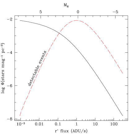
Figure 2: The solid line in this figure shows the R-band luminosity function from Mamon & Soneira (1982). Multiplying this function with the square of the maximum impact parameter $\beta_{\rm max}$ needed to detect a microlensing event gives the dashed line. The line shown is for a detection threshold of 1 ADU s^-1 in r^′. The upper horizontal axis shows absolute R-band magnitude, the lower axis the corresponding r^′ flux.

$\bullet$ Position in M31

Lightcurve quality and detection efficiency vary with position in M31 for several reasons. The photometric sensitivity and therefore the detection efficiency depend on the amount of background light from M31 and are lowest in the the bright central areas of the bulge. Difference images from these areas are also highly crowded with variable-star residuals which influence the photometry and add noise to the microlensing lightcurves. To account for the position-dependence of the detection efficiency, artificial events are generated across the INT fields. To be precise, the artificial event catalogue is constructed in a series of runs. For each run, artificial events are placed on a regular grid with spacing of a 45 pixels ($\simeq 15\,\arcsec$) so that there are 3916 artificial events per chip. The grid is shifted randomly between runs by a maximum of 10 pixels.

Table 2: Fluxes and maximum impact parameters probed in the simulations of microlensing events.

$F_{\rm 0,r}$	$m_{\rm r}$	$F_{\rm 0,i}$	$m_{\rm i}$	$\beta_{\rm u}$
(ADU s-1)		(ADU s-1)
0.01	29.5	0.011	28.75	0.01
0.1	27.0	0.11	26.25	0.09
0.5	25.2	0.55	24.45	0.35
1.0	24.5	1.11	23.75	0.56
10.0	22.0	11.1	21.25	1.67

To summarise, artificial events are characterised by the parameters $t_{\rm FWHM}$, $F_{\rm 0}$, $\mathcal{C}$, $t_{\rm max}$, $\beta$, and their angular position. These events are added as residuals to the difference images using the PSF in the subregion of the event. The residuals also include photon noise. The new difference images are analysed as in Sect. 2 and lightcurves are built for all artificial events detected as variable objects.

4 Microlensing event selection

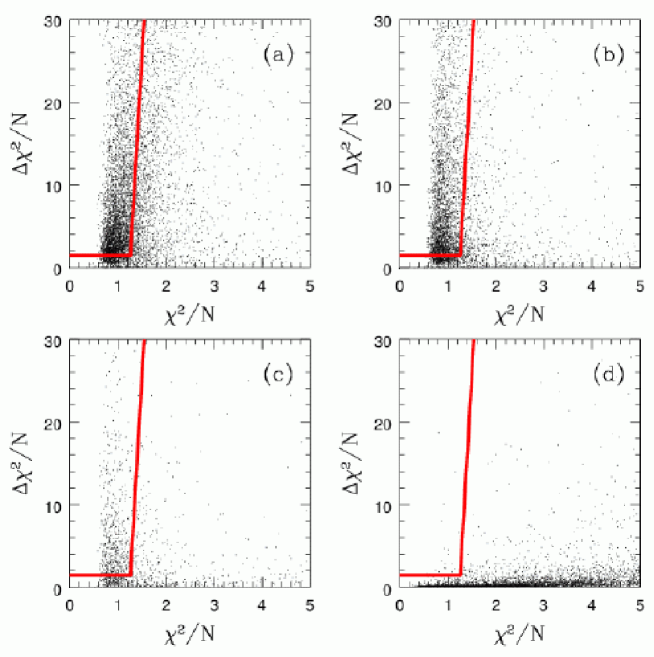
Figure 3: Scatter plots of $\Delta\chi 2$ vs. $\chi 2$ for simulated events with $t_{\rm FWHM}$=50 days (a), 10 days (b), 1 day (c), and for the actual data for 1 CCD. The solid lines correspond to equations 9 and 10.

The vast majority of variable sources in our data set are variable stars. In this section we describe an automated algorithm that selects candidate microlensing lightcurves from this rather formidable background. Our selection criteria pick out lightcurves that have a flat baseline and a single peak with the “correct” shape. The criteria take the form of conditions on the $\chi^{2}$ statistic that measures the goodness-of-fit of an observed lightcurve to equation 4. The fit involves seven free parameters: $t_{\rm max}$, $\beta$, $t_{\rm E}$ , $F_{\rm 0,r}$, $F_{\rm 0,i}$, $\Delta F_{\rm bl,r}$, and $\Delta F_{\rm bl,i}$. To increase computation speed we first obtain rough estimates for $t_{\max}$ and $t_{\rm E}$ from the r^′ lightcurve and then perform the full 7-parameter fit using both r^′ and i^′ lightcurves.

Gravitational lensing is achromatic and therefore the observed colour of a star undergoing microlensing remains constant in contrast with the colour of certain variables. While we do not impose an explicit achromaticity condition, changes in the colour of a variable source show up as a poor simultaneous r^′ and i^′ fit. Because many red variable stars vary little in colour, as defined by measurable differences in flux ratios, the lightcurve shape and baseline flatness are better suited for distinguishing microlensing events from long period variable stars (LPVs) than a condition on achromaticity.

Lightcurves must contain enough information to fit adequately both the peak of the microlensing event and the baseline. We therefore impose the following conditions: (1) The r^′ and i^′ lightcurves must contain at least 100 data points. (2) The peak must be sampled by several points well-above the baseline. (3) The upper half of the peak, as defined in the difference-image lightcurve, must lie completely within a well-sampled observing period. The second condition can be made more precise. We allow for one of the following two possibilities: (a) 4 or more data points in the r^′-lightcurve are $3\sigma$ above the baseline or (b) 2 or more points in r^′ and 1 or more points in i^′ are $3\sigma$ above the baseline. (The r^′ data is weighted more heavily than the i^′ data because it is generally of higher quality and because i^′ was not sampled as well during the first season.) The third condition insures that we sample both rising and falling sides of the peak. We note that there are periods during the last two seasons where we do not have data due to bad weather. The periods we use are the following: 01/08/1999-13/12/1999, 04/08/2000-23/01/2001, 13/08/2001-16/10/2001, 01/08/2002-10/10/2002, and 23/12/2002-31/12/2002.

The selection of candidate microlensing events is based on the $\chi^{2}$-statistic for the fit of the observed lightcurve to equation 4 as well as $\Delta\chi^{2}\equiv\chi^{2}_{\rm flat}-\chi^{2}$ where $\chi^{2}_{\rm flat}$ is the $\chi^{2}$-statistic for the fit of the observed lightcurve to a flat line. Our $\chi^{2}$-cuts are motivated by simulations of artificial microlensing events. In Fig. 3 we show the distribution of artificial events with $t_{\rm FWHM}=50,\,10,\,$ and 1 days (panels a, b, and c respectively) and for all variable sources in one of the CCDs (panel d). In Fig. 4, we show the variable sources from all CCDs that satisfy conditions 1-3. The plots are presented in terms of $\chi^{2}/N$ and $\Delta\chi^{2}/N$ where $N$ is the number of data points in an event. We choose the following cuts:

$$\Delta\chi^{2}>1.5N$$ (9)

and

$$\chi^{2}<\left(N-7\right)f\left(\Delta\chi^{2}\right)+3\left(2\left(N-7\right)\right)^{1/2}$$ (10)

where $f\left(\Delta\chi^{2}\right)=\Delta\chi^{2}/100+1$. The first criterion is meant to filter out peaks due to noise or variable stars. The second criterion corresponds to a $3\sigma$-cut in $\chi^{2}$ for low signal-to-noise events. The $\chi^{2}$ threshold increases with increasing $\Delta\chi^{2}$. Panels a-c of Fig. 3 show a trend where $\chi^{2}$ increases systematically with $\Delta\chi^{2}$. This effect is due to the photometry routine in DIFIMPHOT which underestimates the error in flux measurements for high flux values. The function $f$ is meant to compensate for this effect.

The selection criteria appear as lines in Figs. 3 and 4. (To draw these lines, we take $N=309$ though in practice $N$ is different for individual lightcurves.)

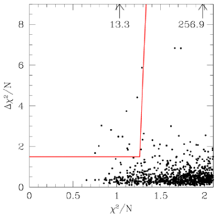
Figure 4: $\Delta\chi^{2}/N$ versus $\chi^{2}/N$ for variable sources that satisfy selection criteria (1), (2) and (3) for peak and lightcurve sampling. The solid line indicates criteria (4) and (5) for peak significance and goodness of fit. Criterium (5) depends on the number of points in the lightcurves, and the line drawn here is for $N$=309, the typical number of available data points per source. Two candidate events with higher $\Delta\chi^{2}/N$ are indicated with arrows, labelled with their $\Delta\chi^{2}/N$ value.

5 Candidate events

Of the 105 477 variable sources 28 667 satisfy conditions 1-3. Of these, 14 meet the criteria set by equations 9 and 10. The positions of 12 of these events in the $\chi^{2}/N-\Delta\chi^{2}/N$ plane are shown in Fig. 4.

5.1 Sample description

In Table 3 we summarise the properties and fit parameters of the 14 candidate microlensing events. The first column gives the assigned names of the events using the nomenclature from Paper I. The numbering reflects the fact that candidates 4, 5, 6, and 12 from Paper I are evidently variable stars since they peaked a second time in the fourth season. The other 10 events from Paper I are “rediscovered” in the current more robust analysis. Four additional candidates, events 15, 16, 17, and 18, are presented. Event 16 is the same as PA-99-N1 from Paulin-Henriksson et al. (2003) and was not selected in our previous analysis because the baseline was too noisy due to a nearby bright variable star. It now passes our selection criteria thanks to the smaller aperture used for the photometry (see discussion below). The three other events all peaked in the fourth observing season and are reported here for the first time.

The coordinates of the events are given in columns 2 and 3 of Table 3; their positions within the INT fields are shown in Fig. 5. The fit parameters, $\chi^{2}$, and $\Delta\chi^{2}$ are given in the remaining columns. In Appendix A we show the r^′ and i^′ lightcurves, thumbnails from the difference images for a number of epochs, and a comparison of $\Delta$r^′ and $\Delta$i^′ for points near the peak. The latter provides an indication of the achromaticity of the event. The lightcurves include data points from observations at the 4m Mayall telescope on Kitt Peak (KP4m) though the fits use only INT data.

Table 3: Coordinates, highest measured difference flux, and some fit parameters for the 14 candidate microlensing events. The peak time $t_{\rm max}$ is in days after August 1st 1999 (JD 2451393).

Candidate	RA	DEC	$\Delta$r′	$t_{\rm max}$	$t_{\rm FWHM}$	$\chi^{2}/N$	$\Delta\chi^{2}/N$	$F_{\rm 0,r}$	r′-i′
event	(J2000)	(J2000)	(mag)	(days)	(days)			(ADU s-1)	(mag)
MEGA-ML 1	0:43:10.54	41:17:47.8	21.8$\pm$0.4	60.1 $\pm$ 0.1	5.4 $\pm$ 7.0	1.12	1.91	0.1$\pm$0.3	0.6
MEGA-ML 2	0:43:11.95	41:17:43.6	21.51$\pm$0.06	34.0 $\pm$ 0.1	4.2 $\pm$ 0.7	1.06	2.48	3.4$\pm$1.7	0.3
MEGA-ML 3	0:43:15.76	41:20:52.2	21.6$\pm$0.1	420.03 $\pm$ 0.03	2.3 $\pm$ 2.9	1.14	2.11	0.08$\pm$0.21	0.4
MEGA-ML 7	0:44:20.89	41:28:44.6	19.37$\pm$0.02	71.8 $\pm$ 0.1	17.8 $\pm$ 0.4	1.98	256.9	6.8$\pm$0.4	1.5
MEGA-ML 8	0:43:24.53	41:37:50.4	22.3$\pm$0.2	63.3 $\pm$ 0.3	27.5 $\pm$ 1.2	0.82	3.03	20.4$\pm$22.9	0.6
MEGA-ML 9	0:44:46.80	41:41:06.7	21.97$\pm$0.08	391.9 $\pm$ 0.1	2.3 $\pm$ 0.4	1.02	2.49	0.9$\pm$0.4	0.2
MEGA-ML 10	0:43:54.87	41:10:33.3	22.2$\pm$0.1	75.9 $\pm$ 0.4	44.7 $\pm$ 5.6	1.28	5.88	1.4$\pm$0.5	1.1
MEGA-ML 11	0:42:29.90	40:53:45.6	20.72$\pm$0.03	488.43 $\pm$ 0.04	2.3 $\pm$ 0.3	1.03	13.27	1.5$\pm$0.4	0.2
MEGA-ML 13	0:43:02.49	40:45:09.2	23.3$\pm$0.1	41.0 $\pm$ 0.3	26.8 $\pm$ 1.5	0.75	1.68	9.2$\pm$10.8	0.8
MEGA-ML 14	0:43:42.53	40:42:33.9	22.5$\pm$0.1	455.9 $\pm$ 0.1	25.4 $\pm$ 0.4	1.11	3.74	146$\pm$182	0.4
MEGA-ML 15	0:43:09.28	41:20:53.4	21.63$\pm$0.08	1145.5 $\pm$ 0.1	16.1 $\pm$ 1.1	1.23	4.41	7.0$\pm$2.2	0.5
MEGA-ML 16	0:42:51.22	41:23:55.3	21.16$\pm$0.06	13.38 $\pm$ 0.02	1.4 $\pm$ 0.1	0.93	2.81	2.6$\pm$0.7
MEGA-ML 17	0:41:55.60	40:56:20.0	22.2$\pm$0.1	1160.7 $\pm$ 0.2	10.1 $\pm$ 2.6	0.79	2.02	0.5$\pm$0.3	0.4
MEGA-ML 18	0:43:17.27	41:02:13.7	22.7$\pm$0.1	1143.9 $\pm$ 0.4	33.4 $\pm$ 2.3	1.13	1.83	13.7$\pm$16.3	0.5

We have already seen that variable stars can mimic microlensing events. Blending of variable stars is also a problem since it leads to noisy baselines. This problem was rather severe in Paper I causing us to miss event PA-99-N1 found by the POINT-AGAPE collaboration (Paulin-Henriksson et al., 2003). In an effort to reduce the effects of blending by variable stars, we use a smaller aperture when fitting the PSF to residuals in the difference images. Nevertheless, some variable star blending is unavoidable, especially in the crowded regions close to the centre of M31. Event 3 provides an example of this effect. A faint positive residual is visible in the 1997 KP4m difference image as shown in Fig. 6. The residual is located one pixel ($0.21^{\prime\prime}$) from the event and is likely due to a variable star. It corresponds to the data point in the lightcurve $\sim$1000 days before the event and well-above the baseline (see Fig. 23). The KP4m data point from 2004 is also above the baseline but in this and other difference images, no residual is visible. The implication is that variable stars can influence the photometry even when they are too faint to be detected directly from the difference images.

fig05.jpg

Figure 5: The locations of the 14 microlensing events within the INT fields are shown here with the dots. Events 7 and 16 correspond with events N2 and N1 from Paulin-Henriksson et al. (2003). Their event S3 is indicated with a cross and lies in the high surface brightness region that we exclude from our analysis. Also marked with a cross (B1) is the position of level 1 candidate 1 of Belokurov et al. (2005).

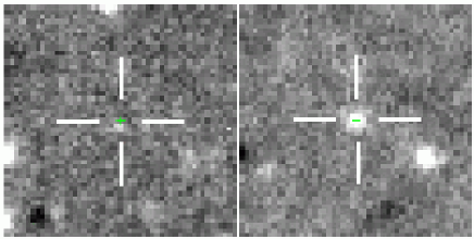
Figure 6: Detail of two KP4m difference images centred on the position of event 3. Left: October 27th 1997, almost 3 years before the event peaks, a very faint residual is seen centred just 1 pixel (0.21″) away from the event. Right: September 26th 2000, during the peak of the event that is displaced from the position of the faint variable.

Good simultaneous fits are obtained in both r^′ and i^′ for all candidate events. Event 7 has a high $\chi^{2}/N$ of 1.98, but since $\Delta\chi^{2}/N$ is very high, the event easily satisfies our selection criteria. In high S/N events, secondary effects from parallax or close caustic approaches can cause measurable deviations from the standard microlensing fit. In addition, as discussed above, we tend to underestimate the photometric errors at high flux levels. An et al. (2004b) studied this event in detail and found that the deviations from the standard microlensing shape of the POINT-AGAPE lightcurve are best explained by a binary lens. The somewhat high $\chi^{2}$ for events 10 and 15 are probably because they are located in regions of high surface brightness.

All of the candidate events are consistent with achromaticity, though for events with low S/N, it is difficult to draw firm conclusions directly from the lightcurves or $\Delta r^{\prime}$ vs. $\Delta i^{\prime}$ plots. The values for $F_{\rm 0,r}$ and $\mathcal{C}$ for the events give some indication of the properties of the source stars. The unlensed fluxes are consistent with the expected range of $0.1-10\,{\rm ADU}\,{\rm s}^{-1}$ and the colours for most of the events are typical of RGB stars. Note however that for many of the events, the uncertainties for $F_{\rm 0}$, $\beta$, and $t_{\rm FWHM}$ are quite large. These uncertainties reflect degeneracies among the lightcurve fit parameters.

The number of candidate events varies considerably from season to season. We find 7 events in the first season, 4 in the second season, none in the third season and 3 in the fourth season. The paucity of events during the third and fourth seasons is not surprising given that we have fewer epochs for those seasons (see table 1). In particular, the gaps in time coverage during those seasons conspired against the detection of short duration events.

5.2 Comparison with other surveys

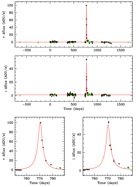
Figure 7: Our photometry for microlensing event candidate 1 from Belokurov et al. (2005).

Figure 8: Relative probability of detecting a microlensing event of a source star with a certain intrinsic flux. This probability is the product of the number of available stars (taken from the luminosity function), the square of the maximum impact parameter for which an event can be detected, and the detection efficiency for each source population, averaged over all $t_{\rm FWHM}$.

The POINT-AGAPE collaboration published several analyses of the INT observations. In Paulin-Henriksson et al. (2003) they presented four convincing microlensing events from the first two observing seasons using stringent selection criteria. In particular, they restricted their search to events with high S/N and $t_{\rm FWHM}<25\,{\rm days}$. They argued that one of these events (PA-00-S3) is probably due to a stellar lens in the M31 bulge. This event lies in the region of the bulge excluded from our analysis (see Fig. 1). The other three events, PA-99-N1, PA-99-N2, and PA-00-S4, correspond respectively to our events 15, 7, and 11. Evidently, the remaining eight events from our analysis of the first two INT seasons did not satisfy their rather severe selection criteria.

In Belokurov et al. (2005), the POINT-AGAPE collaboration analysed data from the first three INT observing seasons without any restrictions on the event duration. Using different selection criteria from their previous analyses, they found three high quality candidates. Two of these events were already known (PA-00-S4 or MEGA-ML-11 and PA-00-S3). The one new event is present in our survey but does not pass our selection criteria because of a high $\chi^{2}$. The lightcurve for this event, along with our best-fit model, is shown Fig. 7. The model does not do a good job of reproducing the observed lightcurve behaviour. In particular, the observed lightcurve appears to be asymmetric about the peak time $t_{\rm max}$. The observed r^′-lightcurve is systematically below the model 15-20 days prior to $t_{\rm max}$. Both r^′ and i^′ lightcurves are above the model 10-15 days after $t_{\rm max}$. Since there are no data available on the rising part of the peak, $t_{\rm max}$ is poorly constrained and may in fact be less than the $770\,{\rm days}$ used in the fit. The shape of our r^′ lightcurve is similar to the one presented in Belokurov et al. (2005) (NB. They removed one epoch close to the peak centre that is present in our lightcurve.) In i^′ the peak shapes are somewhat different.

Peak asymmetries can be caused by secondary effects such as parallax. In our opinion, a more likely explanation for this case is that the event is a nova-like eruptive variable. Granted, the event appears to be achromatic. But classical novae can be achromatic on the declining part of the lightcurve (see, for example, Darnley et al. (2004)), precisely where there is data. If this is a classical nova, it would be a very fast one, with a decline rate corresponding to $\sim$0.6 mag per day.

Figure 9: Detection efficiencies as function of impact parameter $\beta$ for different values of $t_{\rm FWHM}$  (50, 10, 3 and 1 days). The two upper panels show the fraction of simulated events that pass the microlensing selection criteria for 2 source fluxes, 10 and 0.01 ADU s^-1, in the south-east chip of the north field. The lower panels show the same for the south-east chip of the south field.

Calchi Novati et al. (2005) found six candidate microlensing events in an analysis of the three-year INT data set. Of these events, four are the same as reported by Paulin-Henriksson et al. (2003) and two are new events: PA-00-N6 and PA-99-S7. The latter of these is located in the bright part of the southern field excluded in our analysis (Fig. 1). Candidate event PA-00-N6 is present in our data, but was only detected in one epoch in our automatic SExtractor residual detection step and therefore did not make it into the catalogue of variable sources. Calchi Novati et al. (2005) do not detect our events 1, 2, 3, 8, 9, 10, 13, and 14, which all peak in the first two observing seasons. Evidently, these events do not satisfy their S/N constraints.

6 Detection efficiency

We determine the detection efficiency for microlensing events by applying the selection criteria from Sect. 4 to the catalogue of artificial events from Sect. 3. As discussed above, simulated lightcurves are generated by adding artificial events to the difference images and then passing the images through the photometry analysis routine designed for the actual data. Those lightcurves that satisfy the selection criteria for microlensing form a catalogue of simulated detectable microlensing events. The detection efficiency is the ratio of the number of these events to the original number of artificial events.

We first check that our artificial event catalogue includes the portion of the source luminosity function responsible for most of the detectable events. The function $N_{*}\beta_{\rm u}^{2}$ in Fig. 2 is meant to give a qualitative picture of the detectability of microlensing as a function of source luminosity. Here we consider the function $P_{\rm det}\equiv N_{*}\beta_{\rm u}^{2}\epsilon$ where $\epsilon$ is detection efficiency as a function of $F_{0,r}$ integrated over $\beta$, $t_{\rm FWHM}$ and position. $P_{\rm det}$ gives the relative probability for detection of a microlensing event as a function of the source luminosity. As shown in Fig. 8, the range $0.01$ to $10\,{\rm ADU\,s^{-1}}$ adequately covers the peak of this probability distribution.

Our goal is to represent the detection efficiency in terms of a simple portable function of a few key parameters. We adopt a strategy whereby the detection efficiency is modelled as functions of $t_{\rm FWHM}$ and $\Delta F_{\rm max}$ for individual subregions of the two fields. The parameters $\beta$ and $t_{\rm max}$ are “integrated out” and $\mathcal{C}$ is fixed to the value $0.75$. This strategy is motivated by the following considerations.

In Fig. 9 we plot the detection efficiencies as a function of $\beta$ for four different values of $t_{\rm FWHM}$. In each of the panels, the efficiencies are integrated over position within a single chip of the INT fields. The top (bottom) panels are for the south-east chip of the north (south) field. The right (left) panels are for bright (faint) source stars. The general trend is for the detection efficiency to increase with increasing $t_{\rm FWHM}$ and decreasing $\beta$. This trend is expected since longer duration events are more likely to be observed near the peak and smaller values of $\beta$ imply larger amplification factors. For $F(r)=10\,{\rm ADU\,s^{-1}}$, $t_{\rm FWHM}\geq 10\,{\rm days}$ and small $\beta\leq 0.7$, the detection efficiencies decrease with decreasing $\beta$. The decrease is more severe for the $t_{\rm FWHM}=50$ day events where the detection efficiency actually drops below that for the $t_{\rm FWHM}=10$ day events. The problem may be that we underestimate the photometric error at high fluxes therefore causing $\chi^{2}$ to be systematically high. Moreover, $50$ days is a substantial fraction of the observing season and therefore some long duration events may not meet the requirement that the peak be entirely within a single season.

Since the shape of the microlensing lightcurve does not depend strongly on $\beta$ we expect no significant dependence of the detection efficiency on the intrinsic source brightness. This point is illustrated in Fig. 10 where we plot the detection efficiencies as a function of $1/\Delta F_{\rm max}$ for events with $t_{\rm FWHM}=50$ days. We integrate the efficiencies over positions within single CCDs and show the results for four of the eight CCDs in our fields. The curves vary by at most 30% over three orders of magnitude in $F(r)$. The implication is that an explicit $F(r)$ dependence in the detection efficiency will not change the results significantly.

We next test whether the detection efficiency depends on the colour $\mathcal{C}$ of the source. In addition to the main artificial event catalogue, we generate artificial events with $\mathcal{C}=1.25$ and r^′ unchanged for a part of the north field. Fig. 11 compares the detection efficiencies for the two colours and shows that there is no significant difference, except for the very highest signal to noise events. The discrepancy at high S/N reflects the problem discussed above with our estimates of the photometric errors at high flux. This problem is worse for redder sources which have a higher i^′-band flux.

Figure 10: Detection efficiencies as a function of $1/\Delta F_{\rm max}$ for $t_{\rm FWHM}$ = 50 days and $F_{\rm 0,r}$ = 10 ADU s^-1 (solid line), 1 ADU s^-1 (dotted line), 0.1 ADU s^-1 (long-dashed), and 0.01 ADU s^-1 (short-dashed line). In general the lines overlap within the errors.

Figure 11: Colour dependence of the detection efficiency. For $t_{\rm FWHM}$ ’s of 1, 3, 10 and 50 days the detection efficiencies are shown for the 2 different source colours simulated. The colour has no noticeable effect, except for the highest signal-to-noise events.

Figure 12: Detection efficiencies as a function of $1/\Delta F_{\rm max}$ for different values of $t_{\rm FWHM}$. The symbols give the results of the Monte Carlo calculation for one chip. The lines correspond to the fitting formula, equation 11.

Motivated by the shapes of the curves in Fig. 11, we choose a Gaussian in $1/\Delta F_{\rm max}$ where the position of the peak depends on $t_{\rm FWHM}$. The explicit functional form is taken to be:

$$\epsilon\leavevmode\nobreak\ =\leavevmode\nobreak\ c_{1}\left(1-t_{\rm FWHM}/112\right)e^{-c_{2}(1/\Delta F_{\rm max}-c_{3})^{2}}$$ (11)

where

$$c_{3}\leavevmode\nobreak\ =\leavevmode\nobreak\ d_{1}\cdot\ln(t_{\rm FWHM})\leavevmode\nobreak\ +\leavevmode\nobreak\ d_{2}\leavevmode\nobreak\ .$$ (12)

The factor multiplying the Gaussian takes into account the sharp decrease in detection efficiency for events with duration comparable to or longer than the observing season. The parameters $c_{1}$, $c_{2}$, $d_{1}$ and $d_{2}$ are determined by fitting simultaneously the detection efficiencies for all values of $t_{\rm FWHM}$  to equation 11. Fig. 12 shows an example of these fitting formulae to the detection efficiencies.

Fig. 10 illustrates the dependence of the detection efficiencies on location in the INT fields. This dependence is due mainly to variations in galaxy surface brightness but also to the presence of bad pixels and saturated-star defects. As discussed above, we account for the spatial dependence by fitting the detection efficiency separately for subregions of the fields. To be precise, we divide each chip into 32 subregions, $\sim$3′$\times$3′ in size. For each of these regions we average 14 640 simulated events (2 440 per choice of $t_{\rm FWHM}$).

7 Extinction

Microlensing surveys such as MEGA and POINT-AGAPE are motivated, to a large extent, by the argument that a MACHO population in M31 would induce a near-far asymmetry in the microlensing event distribution. In the absence of either extinction or significant intrinsic asymmetries in the galaxy, the distribution of self-lensing events and variable stars masquerading as microlensing events would be near-far symmetric. The detection of a near-far asymmetry would then provide compelling evidence in favour of a significant MACHO population.

Recently, An et al. (2004a) found a near-far asymmetry in the distribution of variables which they attribute to differential extinction across the M31 disk. That differential extinction is significant is also witnessed by several dust features including two prominent dust lanes on the near side of the disk.

We construct a simple model for differential extinction in M31 and test it to against the distribution of LPVs. In the next section, we incorporate this extinction model into our calculations for the theoretical event rate.

Following Walterbos & Kennicutt (1988) we assume that the dust is located in a thin layer in the mid-plane of the disk. Along a given line-of-sight, only light from behind the dust layer is absorbed. Because of the galaxy’s high inclination, the fraction of stars located behind the dust layer is higher for lines-of-sight on the near side of the disk than for those on the far side, as illustrated in Fig. 13. Therefore, even if the distribution of dust is intrinsically symmetric, extinction will have a greater effect on the near side of the disk.

Based on these assumptions the observed intensity along a particular line-of-sight is

$$\mathcal{I}_{\rm obs}\leavevmode\nobreak\ =\leavevmode\nobreak\ \mathcal{I}_{\rm front}\leavevmode\nobreak\ +\leavevmode\nobreak\ \mathcal{I}_{\rm back}e^{-\tau}$$ (13)

where $\mathcal{I}_{\rm front}$ ($\mathcal{I}_{\rm back}$) is the intensity of light originating from in front of (behind) the dust layer and $\tau$ is the optical depth. This equation can be rewritten in terms of the total intrinsic intensity, $\mathcal{I}_{\rm intr}$, and the fraction $x$ of light that originates from in front of the dust layer:

$$\mathcal{I}_{\rm obs}\leavevmode\nobreak\ =\leavevmode\nobreak\ x\mathcal{I}_{\rm intr}\leavevmode\nobreak\ +\leavevmode\nobreak\ (1-x)\mathcal{I}_{\rm intr}e^{-\tau}\leavevmode\nobreak\ .$$ (14)

The three unknowns in this equation, $\mathcal{I}_{\rm intr}$, $x$, and $e^{-\tau}$, depend on wavelength. Rewriting equation 14 for the B-band we have

$$e^{-\tau_{B}}\leavevmode\nobreak\ =\leavevmode\nobreak\ \frac{\mathcal{I}_{\rm obs}(B)/\mathcal{I}_{\rm intr}(B)-x_{B}}{1-x_{B}}.$$ (15)

As a first approximation we assume that $\mathcal{I}_{\rm obs}(I)=\mathcal{I}_{\rm intr}(I)$ so that

$$e^{-\tau_{B}}\leavevmode\nobreak\ =\leavevmode\nobreak\ \frac{\mathcal{I}_{\rm obs}(B)/(\mathcal{C}_{BI}\cdot\mathcal{I}_{\rm obs}(I))\leavevmode\nobreak\ -\leavevmode\nobreak\ x}{1-x}$$ (16)

where $\mathcal{C}_{BI}\equiv\mathcal{I}_{\rm intr}(B)/\mathcal{I}_{\rm intr}(I)$ is the intrinsic $I-B$ colour of the stellar population. An improved estimate of $\mathcal{I}_{\rm intr}(I)$ is obtained by transforming the extinction factor from B to I via the standard reddening law (Savage & Mathis, 1979). The calculation is repeated several times

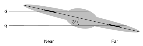
Figure 13: Schematic representation of the line-of-sight through the M31 galaxy from an observer on earth. Because of the high inclination of M31, most of the light observed on the near side of the disk is coming from behind the dust lanes.

We approximate $x_{B}$ and $x_{I}$ from a simple model of the galaxy wherein the intrinsic (i.e., three-dimensional) light distribution $\eta\left({\bf x}\right)$ for the disk and bulge are taken to be double exponentials. In cylindrical coordinates for M31, we have

$$\eta^{i}\left({\bf x}\right)=\eta_{0}e^{-r/h_{R}^{i}}e^{-z/h_{z}^{i}}$$ (17)

where the superscript $i$ denotes either the disk or bulge, $\eta_{0}$ is a normalisation constant, and $h_{R}$ and $h_{z}$ are the radial and vertical scale lengths, respectively. Different scale lengths are used for B and I because the two bands have different sensitivities to young and old populations of stars. Young stars tend to lie closer to the disk mid-plane than old ones. Our choices for the parameters are given in Table 4. The values of the disk scale lengths and the bulge-to-disk-ratios are taken from Walterbos & Kennicutt (1988). The scale lengths for bulge are adapted from their de Vaucouleurs fit while the disk scale heights are based on the distribution of different stellar populations in the Milky Way disk. The observables $\mathcal{I}_{\rm obs}(I)$ and $\mathcal{I}_{\rm obs}(B)$ are from Guhathakurta et al. (2005) who cover a 1.7$\degr\times$5$\degr$ field centred on M31. We derive colour profiles from their mosaics which are found to be similar to the profiles in Walterbos & Kennicutt (1988). The colour is approximately constant within 30$\arcsec$ and becomes bluer at larger radii.

Table 4: Disk and bulge parameters used to derive $x$, the fraction of light originating in front of the mid-plane of M31: the scale length and scale height, $h_{l}$ and $h_{z}$, for disk and bulge, and the fraction of the total light coming from the bulge.

	Disk		Bulge		$L_{\rm b}/(L_{\rm b}+L_{\rm d})$
	$h_{l}$ (kpc)	$h_{z}$ (kpc)	$h_{l}$ (kpc)	$h_{z}$ (kpc)
B	5.8	0.3	1.2	0.75	0.39
I	5.0	0.7	1.2	0.75	0.45

Figure 14: Calculated extinction map in the I-band. Extinction is clearly more severe on the near side of the disk. Note that there are only a few small patches where the extinction factor rises above 40%.

Our I-band extinction map for M31 is shown in Fig. 14. The major dust lanes are clearly visible in the northern field and, as expected, the derived extinction is much larger on the near side of the galaxy than on the far side. The I-band attenuation is $<40\%$ and reaches a maximum in the innermost dust lane and a few smaller complexes.

Our model almost certainly underestimates the effect of extinction across the M31 disk. The approximation $\mathcal{I}_{\rm obs}(I)\simeq\mathcal{I}_{\rm intr}(I)$ is a poor starting point in the limit of large optical depths. For $\tau\gg 1$, most of the light in both B and I from behind the dust layer is absorbed and therefore $\mathcal{I}_{\rm obs}(B)/\mathcal{I}_{\rm obs}(I)\simeq\mathcal{C}_{BI}$. However substituting this result into equation 15 gives $\exp{\left(-\tau\right)}\simeq 1$, an obvious contradiction. By the same token, if the dust is distributed in high-$\tau$ clumps, then $I$ and $B$ wavelengths will be absorbed by equal amounts given essentially by the geometric cross section of the clumps. Moreover, the thin-layer approximation tends to yield an underestimate of the extinction factor (Walterbos & Kennicutt, 1988). Finally, scattering increases the flux observed towards the dust lanes and therefore also leads one to underestimate the extinction factor. Some of these problems can be solved by using infrared data in the construction of the extinction map. In a future paper we plan to use 2MASS data in order to derive a more accurate model for differential extinction in M31.

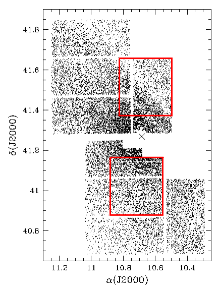
Figure 15: The distribution of the LPVs in M31 with the two symmetrically placed regions used for the LPV amplitude analysis indicated. The northern field is located on the near side and contains some of the most heavily extincted parts, the southern field is on the far side and hardly affected by extinction. These regions are similar to N2 and S2 regions from An et al. (2004a), only adjusted to avoid the part of the southern INT field that is not used in our analysis.

We can use the distribution of variable stars in our survey to test and refine the extinction model. The underlying assumption of this exercise is that the intrinsic distribution of variables is the same on the near and far sides of the disk. We begin by determining the periods of the variable stars using a multi-harmonic periodogram (Schwarzenberg-Czerny, 1996) suitably modified to allow for unevenly sampled data. A six-term Fourier series is then fit to each lightcurve yielding additional information such as the amplitude of the flux variations. Only variables with lightcurves that are well-fit by the Fourier series are used.

We will use LPVs to test the extinction model because they generally belong to quite old stellar populations. This is an advantage because the majority of the microlensing source stars also belong to older populations which are more smoothly distributed over the galaxy than younger variables such as Cepheids. We select LPVs with periods between 150 and 650 days and focus on two regions of our INT fields. One of these is located on the near-side of the disk where extinction is expected to be high while the other is located symmetrically about the M31 centre on the far side. Fig. 15 shows the spatial distribution of the LPVs. Since extinction reduces the amplitude of the flux variations and the average flux by the same factor we can study extinction by comparing the distributions in $\Delta F$ for the near and far sides. These flux variation distributions are shown in Fig. 16. For low $\Delta F$, where the shapes of the distributions are dominated by the detection efficiency, results for the near and far side agree. For high $\Delta F$, where the detection efficiency for variables approaches 100%, one finds a large discrepancy between the near and far-side distributions.

To test whether this discrepancy is indeed due to extinction we transform the coordinates of LPVs on the far side to their mirror image on the near side. The amplitude of the flux variation is then reduced by the model extinction factor suitably transformed from I to r^′ (Savage & Mathis, 1979). The new distribution, shown in Fig. 16, is still significantly above the near-side distribution at large $\Delta F$ though it does provide a better match than the original far-side distribution. The implication is that our model underestimates extinction. To explore this point further we consider models in which $\tau$ is replaced by $c\tau$ where $c>1$. In Fig. 16, we show the distributions of the far side LPVs for $\tau\to 2\tau$ (long-dashed line) and $\tau\to 2.5\tau$ (dot-dashed line). Apparently, the bright end of the (mirror) far-side distribution with $\tau$ increased by a factor of 2.5 agrees with the bright end of the near-side distribution. We therefore conclude that our original model does indeed underestimate the effects of extinction. In some places this will be stronger than in others, but over the probed region the model underestimates extinction effectively by perhaps a factor of 2.5 in $\tau$.

Figure 16: Luminosity functions of LPVs in the 2 symmetrically placed regions. The far side flux distributions were scaled slightly to correct for small differences in area due to the gaps between the CCDs. The solid line is for the near side region and the dotted for the uncorrected far side region. The short-dashed, long-dashed, and dot-dashed lines are far side distributions corrected for increasing levels of extinction.

8 Theoretical predictions

The detection efficiencies found in Sect. 6 allow us to predict the number and distribution of events given a specific model for the galaxy. Though M31 is one of the best studied galaxies, a number of the parameters crucial for microlensing calculations, are not well-known. Chief among these are the mass-to-light ratios of the disk and bulge, $\left(M/L\right)_{\rm d}$ and $\left(M/L\right)_{\rm b}$, respectively. The light distributions for these components are constrained by the surface brightness profile while the mass distributions of the disk, bulge, and halo are constrained by the rotation curve and line-of-sight velocity dispersion profile. However, the mass-to-light ratios are poorly constrained primarily because the shapes of the disk and halo contributions to the rotation curve are similar (e.g. van Albada et al., 1985). One can compensate for an increase in $\left(M/L\right)_{\rm d}$ by decreasing the overall density of the halo. Stellar synthesis models (Bell & de Jong, 2001), combined with observations of the colour profile of M31, can be used to constrain the mass-to-light ratios though these models come with their own internal scatter and assumptions. Another poorly constrained parameter is the thickness of the disk which affects the disk-disk self-lensing rate.

In this section we describe theoretical calculations for the expected number of events in the MEGA-INT survey. We consider a suite of M31 models which span a wide range of values in $\left(M/L\right)_{\rm d}$ and $\left(M/L\right)_{\rm b}$. The dependence of the microlensing rate on other parameters is also explored.

8.1 Self-consistent models of M31

The standard practice for modelling disk galaxies is to choose simple functional forms for the space density of the disk, bulge, and halo tuned to fit observational data. For microlensing calculations, velocity distributions are also required. Typically, one assumes that the velocity distribution for each of the components is isotropic, isothermal, and Maxwellian with a dispersion given by the depth of the gravitational potential or, in the case of the bulge, the observed line-of-sight velocity dispersion. (But see Kerins et al. (2001) where the effects of velocity anisotropy are discussed.) This approach can lead to a variety of problems. First, these “mass models” do not necessarily represent equilibrium configurations, that is, self-consistent solutions to the collisionless Boltzmann and Poisson equations. A system initially specified by the model may well relax to a very different state. Another issue concerns dynamical instability. Self-gravitating rotationally supported disks form strong bars. This instability may be weaker or absent altogether if the disk is supported, at least in part, by the bulge and/or halo. Therefore, models with very high $\left(M/L\right)_{\rm d}$ are the most susceptible to bar formation and can be ruled out.

In order to overcome these difficulties we use new, multi-component models for disk galaxies developed by Widrow & Dubinski (2005). The models assume axisymmetry and incorporate an exponential disk, a Hernquist model bulge (Hernquist, 1990), and an NFW halo (Navarro et al., 1996). They represent self-consistent equilibrium solutions to the coupled Poisson and collisionless Boltzmann equations and are generated using the approach described in Kuijken & Dubinski (1995).

The phase-space distribution functions (DFs) for the disk, bulge, and halo ($f_{\rm disk},\,f_{\rm bulge},\,$ and $f_{\rm halo}$ respectively) are chosen analytic functions of the integrals of motion. For the axisymmetric and time-independent system considered here, the angular momentum about the symmetry axis, $J_{z}$, and the energy, $E$, are integrals of motion. Widrow & Dubinski (2005) assume that $f_{\rm halo}$ depends only on the energy while $f_{\rm bulge}$ incorporates a $J_{z}$-dependence into the Hernquist model DF to allow for rotation. For both halo and bulge, the DFs are “lowered” as with the King model (King, 1966) so that the density goes to zero at a finite “truncation” radius. The disk DF is a function of $E$, $J_{z}$, and an approximate third integral of motion, $E_{z}$, which corresponds to the energy associated with vertical motions of stars in the disk (Kuijken & Dubinski, 1995).

Self-consistency requires that the space density, $\rho$, and gravitational potential, $\psi$, satisfy the following two equations:

$$\rho=\int d^{3}v\left(f_{\rm disk}+f_{\rm bulge}+f_{\rm halo}\right)$$ (18)

and

$$\nabla^{2}\psi=4\pi G\rho\leavevmode\nobreak\ .$$ (19)

Self-consistency is achieved through an iterative scheme and spherical harmonic expansion of $\rho$ and $\psi$. Straightforward techniques allow one to generate an N-body representation suitable for pseudo-observations of the type described below. The N-body representations also provide very clean initial conditions for numerical simulations of bar formation and disk warping and heating.

The DFs are described by 15 parameters which can be tuned to fit a wide range of observations. In addition, one must specify mass-to-light ratios if photometric data is used. Our strategy is to compare pseudo-observations of M31 with actual observational data to yield a $\chi^{2}$-statistic. Minimisation of $\chi^{2}$ over the model parameter space – performed in Widrow & Dubinski (2005) by the downhill simplex method (see e.g. Press et al., 1992) – leads to a best-fit model.

Following Widrow & Dubinski (2005) (see, also Widrow et al. (2003) who carried out a similar exercise with the original Kuijken & Dubinski (1995) models) we utilise measurements of the surface brightness profile, rotation curve, and inner (that is, bulge region) velocity profiles. We use R-band surface brightness profiles for the major and minor axes from Walterbos & Kennicutt (1988). (Widrow & Dubinski (2005) used the global surface brightness profile from Walterbos & Kennicutt (1988) which was obtained by averaging the light distribution in elliptical rings. The use here of both major and minor axis profiles should yield a more faithful bulge-disk decomposition.) The theoretical profiles are corrected for internal extinction using the model described in the previous section. In addition, a correction for Galactic extinction is included. We assume photometric errors of $0.2\,{\rm mag}$. We use a composite rotation curve constructed from observations by Kent (1989) and Braun (1991) that run from 2 to 25 kpc in galactocentric radius. Values and error bars for the circular speed are obtained at intervals of $10\,{\rm arcmin}\simeq 2.2\,{\rm kpc}$ using kernal smoothing (Widrow et al., 2003). Finally, we use kinematic measurements from McElroy (1983) to constrain the dynamics in the innermost part of the galaxy. We smooth his data along the minor axis to give values for the line-of-sight stellar rotation and velocity dispersion at $0.5\,{\rm kpc}$ and $1.0\,{\rm kpc}$. The values at these radii are insensitive to the effects of a central supermassive object and reflect the dynamics of the bulge stars with little disk contamination (McElroy, 1983). An overall $\chi^{2}$ for the model is calculated by combining results from the three types of data. Photometric and kinematic data are given equal weight; the circular rotation curve measurements are weighted more heavily than the bulge velocity and dispersion measurements. To be precise, we use

$$\chi^{2}=\frac{1}{\sqrt{2}}\left(\chi^{2}_{\rm sbp}+\frac{1}{3}\chi^{2}_{\rm disp}+\frac{2}{3}\chi^{2}_{\rm rc}\right)$$ (20)

where $\chi^{2}_{\rm sbp}$, $\chi^{2}_{\rm bulge}$, and $\chi^{2}_{\rm rc}$ are the individual $\chi^{2}$-statistics for the photometric, bulge kinematics, and rotation curve measurements.

Figure 17: Comparison of pseudo-observations of model A1 to real observations. Upper panel: model surface brightness profiles (solid lines) along the major and minor axis compared to observations by Walterbos & Kennicutt (1988) (dots). For clarity the profiles are shifted down in steps of 2 magnitudes. From the top down the profiles correspond to: SW major axis, NE major axis, SE minor axis (far side), and NW minor axis (near side). Lower panel: model rotation curve (solid line) and combined rotation curve from Kent (1989) and Braun (1991). The three lower lines correspond to the contributions to the rotation curve of the bulge (dotted), disk (long dash) and halo (short dash).

Our reference model (model A1) is constructed with $\left(M/L\right)_{\rm d}=2.4$ and $\left(M/L\right)_{\rm b}=3.6$. These values are motivated by the stellar population synthesis models of Bell & de Jong (2001). Along the far side of the minor axis, where the surface brightness profile is relatively free of extinction, the $B-R$ colour is $1.8$ in the bulge region and $1.6$ in the disk region Walterbos & Kennicutt (1988). A correction for Galactic extinction brings these numbers down by $0.18$. Substituting into the appropriate formula from Table 1 of Bell & de Jong (2001) yield the mass-to-light ratios chosen for this model. In Fig. 17 we compare predictions for model A1 with observations. Shown are the surface brightness profiles along major and minor axes and the circular rotation curve. Not shown is the excellent agreement between model and observations for the stellar rotation and dispersion measurements in the bulge region. The reduced $\chi^{2}$ statistic for this model is $1.06$ (see Table 5).

In model A1, the scale height of the disk was fixed to a value of $1.0\,{\rm kpc}$. Note that our model uses a ${\rm sech}^{2}$-law for the vertical structure of the disk. A ${\rm sech}^{2}$-scale height of $1\,{\rm kpc}$ is roughly equivalent to an exponential scale height of $0.5-0.7\,{\rm kpc}$. The observations used in this study do not provide a tight constraint on the scale height of the disk and so we appeal to observations of edge-on disk galaxies. Kregel et al. (2002) studied correlations between the (exponential) vertical scale height and other structural parameters such as the radial scale height and asymptotic circular speed in a sample of 34 edge-on spirals. Using these correlations we arrive at an exponential scale height for $M31$ of $0.6\,{\rm kpc}$ with a fairly large scatter.

We also fix the disk truncation radius for this model to $28\,{\rm kpc}$ which is at the high end of the range favoured in Kregel et al. (2002). Lower values appear to be inconsistent with the measured surface brightness profile. The remaining parameters for the disk, bulge, and halo DFs are varied in order to minimise $\chi^{2}$.

Table 5 outlines other models considered in this paper. Models B1-E1 explore the $\left(M/L\right)_{\rm b}-\left(M/L\right)_{\rm d}$ plane. The $\chi^{2}$ for these models are generally quite low, a reflection of the model degeneracy mentioned above. In these models, disk and bulge “mass” are traded off against halo mass. Previous investigations (Widrow & Dubinski, 2005) suggest that model E1 is unstable to the formation of a strong bar while the other models are stable against bar formation or perhaps allow for a weak bar.

The aforementioned models used values for the extinction factor derived in Sect. 7. As discussed in that section, there are a number of reasons to expect that this model underestimates the amount of extinction in M31. Indeed, our analysis of the near-far asymmetry in LPVs favours a higher optical depth by a factor of $2.5$, that is, the substitution $e^{-\tau}\to e^{-2.5\tau}$. For this reason, we consider a parallel sequence of models, A2-F2, with high extinction. Note that the $\chi^{2}$ for these models are as good as if not better than those for the corresponding low-extinction models.

8.2 Event rate calculation

The event rate is calculated by performing integrals over the lens and source distribution functions. The rate for lenses to enter the lensing tube of a single source is

$$d^{5}R\leavevmode\nobreak\ =\leavevmode\nobreak\ \frac{f_{l}(l_{l},{\bf v}_{l})}{\mathcal{M}_{l}}\leavevmode\nobreak\ 2R_{E}v_{\perp}\leavevmode\nobreak\ dl_{l}d{\bf v}_{l}\leavevmode\nobreak\ d\beta$$ (21)

where $f_{l}$ is the DF for the lens population, $l_{l}$ is the observer-lens distance ($D_{\rm OL}$ in the notation of equation 2), $v_{\perp}$ is the transverse velocity of the lens with respect to the observer-source line-of-sight, and $\mathcal{M}_{l}$ is the mass of the lens. In writing this equation, we assume all lenses have the same mass.

For a distribution of sources described by the DF $f_{s}$, equation 21 is replaced by the following expression for the rate per unit solid angle

$$\frac{dR}{d\Omega}\leavevmode\nobreak\ =\leavevmode\nobreak\ \int\frac{f_{l}(l_{l},{\bf v}_{l})}{\mathcal{M}_{l}}\frac{f_{s}(l_{s},{\bf v}_{s})}{\left(M/L\right)_{s}L_{s}}\leavevmode\nobreak\ 2R_{E}v_{\perp}$$

$$\leavevmode\nobreak\ \times dl_{l}d{\bf v}_{l}\leavevmode\nobreak\ l_{s}^{2}\leavevmode\nobreak\ dl_{s}d{\bf v}_{s}\leavevmode\nobreak\ d\beta$$ (22)

where $l_{s}$ is the observer-source distance, $\left(M/L\right)_{s}$ is the mass-to-light ratio of the source and $L_{s}$ is the source luminosity. (For the moment, we treat all sources as being identical.)

We perform the integrals using a Monte Carlo method. The DFs are sampled at discrete points:

$$f_{p}(l_{p},{\bf v}_{p})\leavevmode\nobreak\ =\leavevmode\nobreak\ \frac{\Sigma_{p}}{N_{p}}\sum_{i=1}^{N_{p}}\delta(l_{p}-l_{i})\leavevmode\nobreak\ \delta({\bf v}_{p}-{\bf v}_{i})$$ (23)

where $p\in\{l,s\}$, $\Sigma_{p}$ is the surface density of either lens or source population, and $N_{p}$ is the number of points used to Monte Carlo either lens or source populations. The nine-dimensional integral in equation 22 is replaced by a double sum and an integral over $\beta$:

$$\frac{dR}{d\Omega}\leavevmode\nobreak\ =\leavevmode\nobreak\ \mathcal{S}_{sl}\sum_{i,j}\int_{0}^{\beta_{u}}d\beta\mathcal{R}_{ij}$$ (24)

where

$$\mathcal{S}_{sl}=\frac{\Sigma_{l}\Sigma_{s}}{N_{l}\mathcal{M}_{l}N_{s}L_{s}\left(M/L\right)_{s}}$$ (25)

and

$$\mathcal{R}_{ij}\leavevmode\nobreak\ \equiv\leavevmode\nobreak\ (2R_{E}v_{\perp})_{ij}l^{2}_{j}\leavevmode\nobreak\ .$$ (26)

Note that $\mathcal{S}$ depends on the line of sight densities of the lens and source distributions along with characteristics of the two populations. $\mathcal{R}_{ij}$ depends on the coordinates and velocities of the lens and source (hence the $ij$ subscripts). The sum is restricted to lens-source pairs with $l_{l}<l_{s}$. For each lens-source pair, the Einstein crossing time, $t_{{\rm E},ij}$ is easily calculated. The differential event rate is then

$$\frac{d^{2}R}{d\Omega dt_{E}}\leavevmode\nobreak\ =\leavevmode\nobreak\ \mathcal{S}_{sl}\sum_{i,j}\int_{0}^{\beta_{u}}d\beta\mathcal{R}_{ij}\delta(t_{{\rm E},ij}-t_{\rm E})\leavevmode\nobreak\ .$$ (27)

8.3 Stellar and MACHO populations

The formulae in the previous section apply to the six lens-source combinations in our model: disk-disk, disk-bulge, bulge-disk, bulge-bulge, halo-disk, and halo-bulge. As written the formulae assume homogeneous populations. For the disk and bulge populations, we modify equation 27 to include integrals over the mass and luminosity functions as appropriate. We write the luminosity function (LF) as

$$\frac{dN}{dM_{R}}\leavevmode\nobreak\ =\leavevmode\nobreak\ Ag(M_{R})\leavevmode\nobreak\$$ (28)

and the mass function as

$$\frac{dN}{d\mathcal{M}}\leavevmode\nobreak\ =\leavevmode\nobreak\ Bh(\mathcal{M},\mathcal{M}_{0})$$ (29)

where $A$ and $B$ are normalisation constants and $\mathcal{M}_{0}$ is the lower bound for the mass function (MF). We take the function $g$ from Mamon & Soneira (1982) and the function $h$ from Binney & Merrifield (1998) (their equation 5.16) with the power-law form $dN/d\mathcal{M}\propto\mathcal{M}^{-1.8}$ extended to $\mathcal{M}_{0}$. $A$ and $B$ are evaluated separately for the disk and bulge populations. In the case of the disk, we assume that $30\%$ of the mass is in the form of gas. The LF is normalised to give $\overline{L}=L_{\odot}$ with the proviso that $L_{s}$ in equation 22 is given in solar units. To determine the normalisation constant $B$ of the mass function, we write

$$Bh(\mathcal{M}_{\odot},\mathcal{M}_{0})\leavevmode\nobreak\ =\leavevmode\nobreak\ \left.\left(\frac{dN}{dM_{V}}\frac{dM_{V}}{d\mathcal{M}}\right)\right|_{\mathcal{M}=\mathcal{M}_{\odot}}$$ (30)

where the V-band LF is again from Mamon & Soneira (1982) and $dM_{V}/d\mathcal{M}$ is from Kroupa et al. (1993). Equation 30 is evaluated at solar values for convenience. The relation

$$\left(\frac{M}{L}\right)_{R}\leavevmode\nobreak\ =\leavevmode\nobreak\ \frac{\int Bh(\mathcal{M},\mathcal{M}_{0})\mathcal{M}d\mathcal{M}}{\int Ag(M_{R})L(M_{R})dM_{R}}$$ (31)

can then be solved for $\mathcal{M}_{0}$. Thus, a disk with high $M/L$ contains more low-mass stars than a disk with low $M/L$.

For simplicity, and because we lack a model for what MACHOs actually are, we assume all MACHOs have the same mass, $\mathcal{M}_{\rm M}$ that is

$$\frac{dN}{d\mathcal{M}}=\delta\left(\mathcal{M}-\mathcal{M}_{M}\right)\leavevmode\nobreak\ .$$ (32)

The value of $\mathcal{M}_{\rm M}$ will directly determine the number density of MACHOs for a given halo mass density. Since the MACHOs only provide lenses and no sources for microlensing, a higher value of $\mathcal{M}_{\rm M}$ and thus a lower number density, will result in a lower number of microlensing events. A given value of $\mathcal{M}_{\rm M}$ can be considered as the average mass of a more elaborate MACHO mass function.

8.4 Theoretical prediction for the number of events

Recall that the efficiency $\epsilon$ is written as a function of $t_{\rm FWHM}$ and $\Delta F_{\rm max}$. (The efficiency also depends on the line of sight.) These quantities are explicit functions of $\beta$, $F_{r}$, and $t_{\rm E}$. Thus, the expected number of events per unit solid angle is

$$\frac{d\mathcal{E}}{d\Omega}=E\,A\,B\mathcal{S}_{ls}\sum_{i,j}\int_{0}^{\beta_{u}}d\beta\int dM_{R}g\left(M_{R}\right)$$

$$\times\int d\mathcal{M}_{l}h\left(\mathcal{M},\mathcal{M}_{0}\right)\mathcal{R}_{ij}\epsilon\left(t_{\rm FWHM},\,\Delta F\right)$$ (33)

where $E$ is the overall duration of the experiment. Our survey covers four half-year seasons and so, with our choice of units for $\epsilon$ and $dR/d\Omega$, we have $E=2$.

The number of events expected in each of the 250 bins used for the extinction calculation and labelled by “k” is

$$\mathcal{E}_{k}=\Delta\Omega\left(\frac{dE}{d\Omega}\right)_{k}$$ (34)

where $\Delta\Omega=9\,{\rm arcmin}^{2}$ is the angular area of a bin. $\mathcal{E}_{k}$ carries an additional label (suppressed for notational simplicity) which denotes the lens-source combination. The total number of events is $\mathcal{E}=\sum\mathcal{E}_{k}$.

8.5 Binary lenses

Our microlensing selection criteria are based on the assumption that the lenses are single point-mass objects. However, at least half of all stars are members of multiple star systems. Microlensing lightcurves for a lens composed of two or more point masses can deviate significantly from the standard lightcurve (Schneider & Weiss, 1986) and may therefore escape detection. The deviations are strongest when the source crosses or comes close to the so-called caustics, positions in the source plane where the magnification factor is formally infinite. (The actual magnification factor is finite due to the finite size of the source.) The size of the caustic region is largest when the separation of the components of the lens is comparable to the Einstein radius corresponding to the total mass (equation 2). Mao & Paczynski (1991) estimated that $\sim$10% of microlensing events towards the bulge of the Milky Way (mainly self-lensing events) should show strong binary characteristics such as caustic crossings. Since the Einstein radius for bulge-bulge self-lensing toward the Milky Way and M31 are comparable, we can expect a similar 10% effect in our survey. Baltz & Gondolo (2001) perform a similar analysis for pixel-lensing surveys and estimate that in the order of 6% of self-lensing events from normal stellar populations will exhibit caustic crossings. Since the majority of detected events will have low signal-to-noise, we can assume that deviations other than caustic crossings in most cases will not strongly affect our detection efficiency. Therefore, to account for binary lenses, the calculated theoretical predictions for self-lensing are revised downward by $10\%$.

8.6 Results

Table 5 presents the theoretical predictions for the total number of events expected in the MEGA-INT four-year survey. The results are given for both self-lensing ($\mathcal{E}_{\rm self}$) and halo lensing ($\mathcal{E}_{\rm halo}$). The values quoted for $\mathcal{E}_{\rm halo}$ assume 100% of the halo is in the form of MACHOs. In other words, these values should be multiplied by the MACHO halo fraction in order to get the expected number of events for a MACHO component. We note that lensing by the Milky Way halo is not included in these results. This possible contribution is expected to be small, since the number of microlensing events from a 100% MW halo is a few times lower than for a 100% M31 halo (Gyuk & Crotts, 2000; Baillon et al., 1993) for MACHO masses around 0.5M_⊙.

We also consider the near-far asymmetry for self and halo lensing. In Fig. 18, we show the cumulative distribution of events for self and halo lensing as a function of the distance from the major axis, $s$. We take $s$ to be positive on the far side of the disk. For this plot, we choose model A1 but since the distributions are normalised to give 14 total events, the difference between the models is rather inconsequential. We see that both self and halo lensing models do a good job of describing the event distribution in the inner $0.2^{\circ}$. The halo distribution does a somewhat better job of modelling the three events between $s=0.2^{\circ}$ and $s=0.3^{\circ}$. Neither halo nor self lensing models predict anywhere near two events for $s>0.35^{\circ}$.

To further explore the distribution, we define the asymmetry parameter $\mathcal{A}$:

$$\mathcal{A}\leavevmode\nobreak\ =\leavevmode\nobreak\ \frac{\sum\mathcal{E}_{k}\cdot s_{k}}{\mathcal{E}}\leavevmode\nobreak\ .$$ (35)

In Table 5 we give values for $\mathcal{A}_{\rm self}$ and $\mathcal{A}_{\rm halo}$. We also provide an average $\mathcal{A}_{\rm ave}$ which assumes that MACHOs make up the shortfall between the expected number of events and the observed value of 14. In cases where the expected number of events is greater than 14, we set $\mathcal{A}_{\rm ave}=\mathcal{A}_{\rm self}$. The asymmetry parameter for the 14 candidate events is $\mathcal{A}_{\rm data}=0.125$.

Table 5: Results of the microlensing modelling using self-consistent M31 models. In the first columns some model parameters and the combined $\chi^{2}$ are listed. The remaining columns contain the predicted number of events due to self-lensing ($\mathcal{E}_{self}$), due to halo-lensing ($\mathcal{E}_{halo}$), the asymmetry of the self-lensing ($\mathcal{A}_{self}$), of the halo-lensing ($\mathcal{A}_{halo}$), and of the combination of both ($\mathcal{A}_{ave}$). The number of self-lensing events $\mathcal{E}_{self}$ has been corrected for the fact that $\sim$10% of the events will show strong binary effects and therefore be selected against. The microlensing event rate due to the halo $\mathcal{E}_{halo}$ is for a 100% MACHO halo, i.e. all of the halo mass is assumed to be in the MACHOs. For calculating the combined self- and halo-lensing asymmetry parameter $\mathcal{A}_{ave}$ a smaller fraction of the halo mass is assumed to be in MACHOs, namely the amount necessary to make up the difference, if any, between $\mathcal{E}_{self}$ and the observed number of 14 candidate events. The disk scale heights $h_{z}$ are $sech^{2}$ scale heights. The upper, low extinction part of the table contains models with internal extinction values as derived in section 7, while the lower, high extinction part contains models with increased extinction, as motivated by our analysis of the LPV amplitudes.

Low extinction
Models with $m_{\textsc{macho}}$=0.5 M⊙ and $h_{z}$=1.0 kpc
	$(M/L)_{\rm d}$	$(M/L)_{\rm b}$	$\chi^{2}$	$\mathcal{E}_{\rm self}$	$\mathcal{E}_{\rm halo}$	$\mathcal{A}_{\rm self}$	$\mathcal{A}_{\rm halo}$	$\mathcal{A}_{\rm ave}$
A1	2.4	3.6	1.06	14.2	30.9	0.037	0.086	0.037
B1	2.4	2.9	1.17	13.4	31.5	0.031	0.085	0.033
C1	2.4	4.3	1.02	13.1	29.6	0.039	0.092	0.043
D1	1.8	2.4	1.34	11.3	35.5	0.031	0.082	0.041
E1	3.6	4.4	1.03	15.8	24.6	0.030	0.091	0.030
Models with $(M/L)_{\rm d}$=2.4 and $(M/L)_{\rm b}$=3.6
	$h_{z}$	$\mathcal{M}_{\rm M}$	$\chi^{2}$	$\mathcal{E}_{\rm self}$	$\mathcal{E}_{\rm halo}$	$\mathcal{A}_{\rm self}$	$\mathcal{A}_{\rm halo}$	$\mathcal{A}_{\rm ave}$
F1	0.5	0.5	1.10	12.5	30.7	0.037	0.084	0.042
G1	1.0	0.1	1.06	14.2	43.1	0.037	0.088	0.037
H1	1.0	1.0	1.06	14.2	25.9	0.037	0.085	0.037
High extinction
Models with $\mathcal{M}_{\rm M}=0.5M_{\odot}$ and $h_{z}$=1.0 kpc
	$(M/L)_{\rm d}$	$(M/L)_{\rm b}$	$\chi^{2}$	$\mathcal{E}_{\rm self}$	$\mathcal{E}_{\rm halo}$	$\mathcal{A}_{\rm self}$	$\mathcal{A}_{\rm halo}$	$\mathcal{A}_{\rm ave}$
A2	2.4	3.6	0.99	12.4	28.6	0.052	0.095	0.057
B2	2.4	2.9	1.08	12.2	32.6	0.046	0.094	0.052
C2	2.4	4.3	0.99	14.5	29.6	0.056	0.098	0.056
D2	1.8	2.4	1.23	10.3	34.5	0.045	0.095	0.058
E2	3.6	4.4	1.04	14.2	22.8	0.046	0.105	0.046
Models with $(M/L)_{\rm d}$=2.4 and $(M/L)_{\rm b}$=3.6
	$h_{z}$	$\mathcal{M}_{\rm M}$	$\chi^{2}$	$\mathcal{E}_{\rm self}$	$\mathcal{E}_{\rm halo}$	$\mathcal{A}_{\rm self}$	$\mathcal{A}_{\rm halo}$	$\mathcal{A}_{\rm ave}$
F2	0.5	0.5	1.06	11.2	30.5	0.052	0.095	0.061
G2	1.0	0.1	0.99	12.4	39.1	0.052	0.098	0.057
H2	1.0	1.0	0.99	12.4	23.8	0.052	0.093	0.057

The general trend, in terms of total expected number of events, is that as the mass-to-light ratios are increased, $\mathcal{E}_{\rm self}$ increases and $\mathcal{E}_{\rm halo}$ decreases. There are counter examples. In model C1, the $\left(M/L\right)_{\rm b}$ (as compared with model A1) leads to a less massive disk and lower $\mathcal{E}_{\rm self}$. Recall that for each choice of mass-to-light ratios, the remaining parameters are adjusted to minimise $\chi^{2}$. The process can lead to rather complicated interdependencies between the model parameters. The self-lensing rate decreases with decreasing $h_{z}$ as illustrated with model F1. The self-lensing rate is generally reduced in the high extinction models relative to the low extinction ones. Finally we see that the halo event rate decreases with increasing MACHO mass. Models G and H illustrate this point and span the range in $\mathcal{M}_{M}$ identified by Alcock et al. (2000) as the most probable mass range for Milky Way MACHOs.

The timescale distribution is easily calculated using the method outlined in the previous section. Essentially, one calculates $t_{\rm FWHM}$ for each lens-source pair in the Monte Carlo sum. In Fig. 19 we show the cumulative timescale distribution of our candidate microlensing event sample and model A1. In constructing the curves for self and halo lensing, we have scaled the distributions to give a total of 14 events.

Figure 18: Cumulative event distribution as a function of distance from the major axis (in degrees). Shown are the data (dots), self-lensing distribution (solid line), and halo-lensing distribution (dotted line). Both self- and halo-lensing lines are scaled to give a total of 14 events.

Figure 19: Cumulative microlensing event distribution as a function of timescale. The line and point-types are the same as in Fig. 18.

9 Discussion

The numbers expected for events due to self-lensing across the models probed in Table 5 fall within the narrow range of 10-16. The relative insensitivity of $\mathcal{E}_{\rm self}$ to changes in the mass-to-light ratios is a result of our approach to constructing models; changes in $\left(M/L\right)_{\rm b}$ and $\left(M/L\right)_{\rm d}$ are compensated by changes in the structural parameters of the disk, bulge, and halo so as to minimise $\chi^{2}$ for the fit to the rotation curve and surface brightness data. Consider models D1 and E1. The mass-to-light ratios differ by a factor of $\sim 2$ while $\mathcal{E}_{\rm self}$ differs by only a factor of 1.4; with the low $M/L$ values in model D1, the rotation curve data drive up the disk and bulge luminosity distributions at the expense of a poorer fit for the photometric data. A balance is struck and the net result is that the change in $\mathcal{E}_{\rm self}$ is significantly smaller than what one might expect.

The consistency of the number of candidate events with the number of predicted self-lensing events is contrary to the results of the analysis of the first three seasons of INT data by the POINT-AGAPE collaboration. Calchi Novati et al. (2005) present six high quality, short duration microlensing candidates with one of these events attributed to M32-M31 lensing. They also model the detection efficiency and calculate number of expected self- and halo-lensing events for a variety of M31 models. In all of their models, the number of events for self-lensing is predicted to be less than $\sim 1.5$. Since this number is significantly less than the observed number, they conclude that some of the events are due to MACHOs and estimate that the MACHO halo fraction is at least 20%.

Calchi Novati et al. (2005) use the model from Kerins et al. (2001) which features a bulge following Kent (1989), an exponential $sech^{2}$ disk and a spherical, nearly isothermal halo. They use the same structural parameters for the three components as Kerins et al. (2001) but take $(M/L_{B})_{b}=3$ and $(M/L)_{d}=4$. This model for the stellar mass distribution in M31 predicts an inner rotation curve that is significantly lower than the observed one, and so an extra ‘dark bulge’ component is required as well as the isothermal halo. Calchi Novati et al. (2005) do not consider microlensing by this dark bulge in their model, but instead attribute all surplus microlensing to the halo. In our model the stellar bulge is more massive, with $M/L$ that is sufficient to reproduce the inner rotation curve, and there is no non-lensing dark bulge component. It appears to provide sufficient microlensing events to explain the observations.

Furthermore, the choice of $0.3\,{\rm kpc}$ for the $sech^{2}$ scale height is small by perhaps a factor of 3 if M31 is a typical spiral galaxy as represented in the survey by Kregel et al. (2002). Thickening the disk increases the disk-disk self-lensing rate.

For our models, the number of events due to self-lensing is consistent with the total number of events observed but not inconsistent with a significant MACHO fraction for the halo of M31. We can make this statement more quantitative by treating halo events as a Poisson process with background due to self-lensing and employing the approach of Feldman & Cousins (1998). We let $n$ be the number of observed events consisting of MACHO events with mean $f\mathcal{E}_{\rm halo}$, where $f$ is the MACHO fraction, and a background due to self-lensing with known mean $\mathcal{E}_{\rm self}$. For this analysis, we ignore the background due to variables and background supernovae. The probability distribution function is

$$P\left(n|f\right)=\left(f\mathcal{E}_{\rm halo}+\mathcal{E}_{\rm self}\right)^{n}\exp\left[-\left(f\mathcal{E}_{\rm halo}+\mathcal{E}_{\rm self}\right)\right]/n!\leavevmode\nobreak\ .$$ (36)

To obtain confidence intervals for $f$:

1. Calculate $P\left(n|f\right)$ for $N$ values of $f\in\{0,1\}$ and sort from high to low. The maximum of $P$ defines the most probable value of $f$. The values of $P$ are normalised so that the sum of all sampled values of $P$ is 1.

2. Accept values of $f$ starting from the highest value of $P$ until the sum of $P$ exceeds the desired confidence level. The largest and smallest values of accepted $f$ define the confidence interval.

In Table 6 we provide most probable values of $f$ and 95% confidence intervals for all of the models in Table 5. We provide these values both for the case of the full sample of 14 observed candidate events ($n$=14), as well as for the case of 11 observed events ($n$=11), for reasons discussed below.

We next turn to the distribution of events across the M31 disk as represented by the asymmetry parameters. From Table 5 we see that $\mathcal{A}_{\rm self}<\mathcal{A}_{\rm halo}<\mathcal{A}_{\rm data}$. The (weak) asymmetry in the self-lensing distribution is due to extinction. Note that the values are significantly below $\mathcal{A}_{\rm data}$ even for the high extinction models.

The asymmetry parameter for the halo is significantly higher than that for self-lensing events and close to, though still below, $\mathcal{A}_{\rm data}$. However, the asymmetry parameter for combinations of self and halo lensing are well below $\mathcal{A}_{\rm data}$. Evidently, the distribution of candidate events is difficult to explain with any reasonable combination of self and halo lensing.

The large asymmetry in the data is due, for the most part, to events 11, 13, and 14 (see Table 7). It is therefore worth considering alternative explanations for these events. As argued in Paulin-Henriksson et al. (2002), the lens for event 11 likely resides in M32 and since we have not included M32 in our model, this event should be removed from the analysis. Doing so leads to a modest reduction in $\mathcal{A}_{\rm data}$.

Events 13 and 14 may be more difficult to explain. For model A1, the predicted number of self-lensing events with $s>s\left({\rm event}\,18\right)$ is $0.005$ while the predicted number of MACHO events in the same range in $s$ is $0.14f$. Thus, the probability of having two events either from self or halo lensing is exceedingly small, unless the halo fraction is very large. However, since some contamination by variable stars of our sample can not be excluded, one or both of these events may be a variable star. We note, for example, that event 13 has the lowest S/N in our sample. The probability of having one event for MACHO lensing with $f=0.20$ is $\sim 3\%$, small, but not vanishingly so.

A closer inspection of the model is also warranted. Recall that our models assume axisymmetry whereas M31 exhibits a variety of non-axisymmetric features such as disk warping. This point is illustrated in the isophotal map by Hodge & Kennicutt (1982). From the map, one finds that event 13 lies on the B=24 (R=22.6) contour while model A1 predicts R=23.5. Thus, the model may in fact underestimate the surface brightness of the disk by a factor of 2, and hence the disk-disk self-lensing rate by a factor of 4. (The reason for the discrepancy is not completely clear. The contours on the far side do appear to be “boxier” than those predicted by the model.)

It is interesting to note that events 13 and 14 are coincident with the location of the giant stellar stream discovered by Ibata et al. (2001). This stream runs across the southern INT field, approximately perpendicular to the major axis and over M32. Indeed, M32 may be the progenitor of the stream (Merrett et al., 2003). The average V-band surface brightness of the stream is $\Sigma_{V}\approx 30\pm 0.5$ mag arcsec^-2 (Ibata et al., 2001) but this is measured far from the projected positions of events 13 and 14. The surface brightness of the stream might be significantly higher near the position of M32. Perhaps the most conservative statement one can make about the stream is that it is not bright enough to distort the contours near events 13 and 14, that is, it cannot be brighter than the disk at these radii. The microlensing event rate due to stars in the stream is of course enhanced relative to the rate for self-lensing by the ratio of the distance from the stream to the disk and the thickness of the disk, that is, by a factor of $\sim 20$. The stream-disk lensing rate might be further enhanced if the stars in the stream have a large proper motion relative to the disk. These arguments suggest that the number of stream-disk events in the vicinity of M32 might be $0.03-0.1$; perhaps high enough to explain one event.

Table 6: Most probable value and 95% confidence limits for the MACHO halo fraction $f$ from the Feldman & Cousins (1998) analysis, for the full sample and the case without candidate events 11, 13, and 14.

	14 events		11 events
model	$f_{\rm best}$	conf. interval	$f_{\rm best}$	conf. interval
A1	0.	[0,0.28]	0.	[0.,0.21]
B1	0.02	[0,0.29]	0.	[0.,0.22]
C1	0.03	[0,0.32]	0.	[0.,0.24]
D1	0.08	[0,0.30]	0.	[0.,0.22]
E1	0.	[0,0.32]	0.	[0.,0.25]
F1	0.05	[0,0.32]	0.	[0.,0.24]
G1	0.	[0,0.20]	0.	[0.,0.15]
H1	0.	[0,0.34]	0.	[0.,0.25]
A2	0.06	[0.,0.35]	0.	[0.,0.25]
B2	0.06	[0.,0.31]	0.	[0.,0.23]
C2	0.	[0.,0.29]	0.	[0.,0.22]
D2	0.11	[0.,0.33]	0.02	[0.,0.24]
E2	0.	[0.,0.39]	0.	[0.,0.29]
F2	0.09	[0.,0.35]	0.	[0.,0.26]
G2	0.04	[0.,0.25]	0.	[0.,0.18]
H2	0.07	[0.,0.42]	0.	[0.,0.31]

Table 7: Observed number of events and the asymmetry of their spatial distribution, shown for the full sample of 14 events and for cases where the probable M32 event (11) and candidate events 13 and 14 are ignored. The quoted errors are 1$\sigma$ errors, determined with the bootstrap method. Also shown is the asymmetry for the long-period variable stars (LPVs).

Events used	$\mathcal{E}_{data}$	$\mathcal{A}_{data}$
Full sample	14	0.125 $\pm$ 0.046
without 11	13	0.120 $\pm$ 0.049
without 13, 14	12	0.076 $\pm$ 0.034
without 11, 13, 14	11	0.066 $\pm$ 0.034
LPVs	20,864	0.071 $\pm$ 0.001

Figure 20: Asymmetries and event numbers for data and models. The points with error bars on the left show $\mathcal{E}$ and $\mathcal{A}$ for the sample of candidate events and the subsamples listed in table 7. The solid lines correspond to the high and the dotted lines to the low extinction models from table 5. The dots are the pure self-lensing points, with the MACHO mass fraction increasing along the line. MACHO fractions of 20% are indicated with vertical lines.

Fig. 20 provides a summary of our results with respect to the expected number of events and the asymmetry parameter. The points with error bars represent the data for the 4 cases considered in Table 7. The solid circles and lines correspond to the high extinction case; the open circles and dotted lines correspond to the low extinction case. The circles assume pure self lensing while the lines trace out the values for increasing MACHO fraction with the tick-mark indicating the position of $f=0.2$. Once again, we see that the asymmetry parameter for the data is higher than that for any of the models. Removing events 13 and 14 does improve the situation as does increasing the optical depth $\tau$; the asymmetry remains a little higher but consistent with the models.

10 Conclusions

This paper presents the analysis of four seasons of M31 observations at the INT, a subset of the MEGA survey of M31. The observations were carried out to search for MACHOs in the halo of M31. Our fully automated search algorithm identified 14 candidate microlensing events from over $10^{5}$ variable sources. Three of the candidates were previously unpublished. The spatial and timescale distributions are consistent with microlensing.

The core of this paper is the comparison of this candidate event sample with a calculation of the expected number of events from self and halo lensing. This calculation breaks into three parts: a model for the extinction across the M31 disk; a model for the detection efficiency; and a suite of self-consistent disk-bulge-halo models for M31.

The results with regard to the fundamental question of whether there is a significant MACHO fraction in the halo are inconclusive. Based on the total number of events, we find that the most probable MACHO halo fraction $f$ varies between $0$ and $0.1$ depending on the model. Our event rate analysis is consistent with a total absence of MACHOs as the confidence intervals for all of our models include $f=0$. On the other hand we can not exclude some MACHO component, since the confidence intervals extend typically up to $f=0.25$ and even up to $f=0.4$ for a few models.

The spatial distribution of the candidate events is highly asymmetric and does seem to favour a MACHO component. However, for different reasons it is questionable whether the 3 candidate events that largely determine the asymmetry signal should be used in this analysis. Thus, we conclude that both from the observed number of events, and from their spatial distribution we find no compelling evidence for the presence of MACHOs in the halo of M31.

Appendix A Candidate event lightcurves

On the following pages, for each of the 14 candidate microlensing events in our sample, the r^′ and i^′ lightcurves and thumbnails taken from the difference centred on the event positions are shown, together with a short discussion. Apart from the INT r^′ and i^′ data, KP4m R and I data points are also plotted in the lightcurves. The fits shown are however the fits done to only the INT data.

figapp01a.gif

Figure 21: (a) Event 1: lightcurves. The two upper panels show the full r^′ and i^′ lightcurves of the microlensing event. In the lower left corner are zooms on the peak region. In the lower right corner the r^′ flux is plotted versus the i^′ flux; if the colour is constant, the points should lie on a straight line. Also drawn is the best fit microlensing model. The solid circles are points from the INT data, the open circles are from the KP4m data. The start of the INT survey, August 1st 1999, is used as the zeropoint for the timescale.

figapp01b.jpg

Figure 21: (b) Event 1: thumbnails. The two upper rows of thumbnails show are taken from r^′ and i^′ difference images during the peak of the candidate event. Selected thumbnails from the baseline are also shown in the two bottom rows. Each thumbnail is 30$\times$30 pixels or 10$\times$10″  in size.

MEGA-ML-1

Located close to the centre of M31, this event has a rather noisy baseline. Apart from the background of very faint variables there are some variable sources clearly visible in the difference images. As can be seen in the thumbnails in figure 21(b) a bright variable is located just a few pixels from the position of the candidate event. Another, fainter variable is seen at a similar distance above and to the left. The other variable sources are further away and should have no influence on the photometry.

figapp02a.gif

Figure 22: (a) Event 2: lightcurves. See caption of 21(a).

figapp02b.jpg

Figure 22: (b) Event 2: thumbnails. See caption of 21(b).

MEGA-ML-2

This candidate event is located very close to MEGA-ML-1 and therefore has the same problems connected to being close the centre of M31. In the thumbnails of days 94, 754, and 1208 we see a variable source a few pixels to the left of the event position. This variable is brighter in r^′ than in i^′, which causes the r^′ baseline to be the most noisy.

figapp03a.gif

Figure 23: (a) Event 3: lightcurves. See caption of 21(a).

figapp03b.jpg

Figure 23: (b) Event 3: thumbnails. See caption of 21(b).

MEGA-ML-3

This candidate event is also located close to the M31 centre. In figure 6 we already demonstrated that a very faint variable source is positioned $\sim$0.25″away from this candidate event. In the i^′ thumbnails another variable is visible just above and to the right of the event. This variable has a bright episode between days 440 and 480, causing the bump in the baseline in the i^′ lightcurve.

figapp04a.gif

Figure 24: (a) Event 7: lightcurves. See caption of 21(a).

figapp04b.jpg

Figure 24: (b) Event 7: thumbnails. See caption of 21(b).

MEGA-ML-7

By far the brightest event in our sample, the thumbnails of MEGA-ML-7 show a very bright residual close to the peak centre. Since the peak occurs during the first season, some of the exposures used for creating the reference image contained a significant amount of the magnified flux, so that the baseline lies at a negative difference flux. There are some variables nearby, but none of them are close or bright enough to significantly influence the photometry. The distance to the centre of M31 is also quite large ($\sim$22′), reducing the background of faint variable sources. As pointed out by Paulin-Henriksson et al. (2003), there are some systematic deviations from the best fit microlensing model. An et al. (2004c) find that this anomaly can be explained by a binary lens.

figapp05a.gif

Figure 25: (a) Event 8: lightcurves. See caption of 21(a).

figapp05b.jpg

Figure 25: (b) Event 8: thumbnails. See caption of 21(b).

MEGA-ML-8

This near side event is located $\sim$23′  from the centre of M31. A variable that is particularly bright in i^′ is situated about 2.4″  NW of the candidate event, but should not have much of an effect on the photometry. The baselines of the lightcurves indeed look stable and well-behaved.

figapp06a.gif

Figure 26: (a) Event 9: lightcurves. See caption of 21(a).

figapp06b.jpg

Figure 26: (b) Event 9: thumbnails. See caption of 21(b).

MEGA-ML-9

Peak coverage is poor for this candidate event, but the baselines are stable. The thumbnails show quite a lot of faint variables, two of which are located very close, approximately 1″  to the left of the event position, accounting for the noise in the i^′ baseline that is higher than in the r^′ lightcurve.

figapp07a.gif

Figure 27: (a) Event 10: lightcurves. See caption of 21(a).

figapp07b.jpg

Figure 27: (b) Event 10: thumbnails. See caption of 21(b).

MEGA-ML-10

This event is a beautiful example of a combined lightcurve with KP4m and INT data. Peak coverage in INT i^′ is poor, but the KP4m I data points follow the fit (derived only from INT data) very well. A fairly bright variable is situated slightly above and to the right of the event position and there is a hint of a very faint variable about 1″  to the left. Although the INT baseline in i^′ is noisy, the r^′ and both KP4m R and I lightcurves show an very stable and well-behaved baseline.

figapp08a.gif

Figure 28: (a) Event 11: lightcurves. See caption of 21(a).

figapp08b.jpg

Figure 28: (b) Event 11: thumbnails. See caption of 21(b).

MEGA-ML-11

A high signal-to-noise event with a good fit and stable baseline. There is some noise in the i^′ baseline, caused by the variable source that is visible in the thumbnails of days 6 and 756 at $\sim$1.3″  above the event position. During the fourth observing season a few bad columns were lying exactly on top of the event position, so that there is only 1 INT data point available. However, the KP4m data show that the baseline remains flat everywhere.

figapp09a.gif

Figure 29: (a) Event 13: lightcurves. See caption of 21(a).

figapp09b.jpg

Figure 29: (b) Event 13: thumbnails. See caption of 21(b).

MEGA-ML-13

This candidate event has the lowest signal-to-noise of our sample. It is situated far out in the far side of the disk at $\sim$31′  from the centre of the galaxy and the relatively low galaxy background makes it possible to detect these kind of faint events. Due to the y-axis scale the i^′ the baseline looks quite noisy, but it is in fact not significantly more so than for other candidate events. The thumbnails of days 398 and 520 show that the closest variable source is located $\sim$1.4″  below and to the left of the event, which explains the scatter in the i^′ baseline.

figapp10a.gif

Figure 30: (a) Event 14: lightcurves. See caption of 21(a).

figapp10b.jpg

Figure 30: (b) Event 14: thumbnails. See caption of 21(b).

MEGA-ML-14

At $\sim$35.5′  from the M31 centre, this candidate event is the most far out in the disk of all events in our sample. The i^′ photometry of this candidate event is compromised by the variable source at $\sim$1.3″. From the i^′ thumbnails one can also see that the event lies at the edge of a fringe, making the background in the lower half of the thumbnails brighter than in the upper half. This can also cause some extra scatter in the photometry. Overall, however, the microlensing fit is very good and both INT and KP4m lightcurves show a stable baseline.

figapp11a.gif

Figure 31: (a) Event 15: lightcurves. See caption of 21(a).

figapp11b.jpg

Figure 31: (b) Event 15: thumbnails. See caption of 21(b).

MEGA-ML-15

This event is again located close to the centre of M31 and presumably has a strong background of faint variable sources. In the thumbnails also several variables are visible very close to the event position, both in r^′ and in i^′. The lightcurve baselines are rather noisy because of this, but show no coherent secondary bumps and the KP4m baselines are very stable.

figapp12a.gif

Figure 32: (a) Event 16: lightcurves. See caption of 21(a).

figapp12b.jpg

Figure 32: (b) Event 16: thumbnails. See caption of 21(b).

MEGA-ML-16

Not selected in our first analysis of the first two seasons of INT data (de Jong et al. 2004) due to baseline variability, the i^′ lightcurve of this event is strongly influenced by a bright variable situated just 1.1″  to the north. Using a smaller extraction aperture for the photometry in the present analysis, the i^′ baseline is still very noisy and the same is true for the KP4m I-band data. The INT r^′ and KP4m R data are much better behaved and the r^′ peak is fit very well by the microlensing fit.

figapp13a.gif

Figure 33: (a) Event 17: lightcurves. See caption of 21(a).

figapp13b.jpg

Figure 33: (b) Event 17: thumbnails. See caption of 21(b).

MEGA-ML-17

The i^′ baseline is slightly noisy, but the r^′ and both KP4m lightcurves are well-behaved. In the thumbnails no very close variables are visible.

figapp18a.gif

Figure 34: (a) Event 18: lightcurves. See caption of 21(a).

figapp18b.jpg

Figure 34: (b) Event 18: thumbnails. See caption of 21(b).

MEGA-ML-18

This candidate event shows quite large scatter in the baseline and also in the peak. Faint variables might be the culprits, although the event is not located very close to the galaxy centre ($\sim$15.1′). The thumbnails show no variable sources very close to the event position, however they do show that this event is situated on the edge of a fringe running diagonally across the thumbnails. This fringe and the fact that it can change position slightly between frames is the most probable cause for the noisy i^′ photometry.