A VSA search for the extended Sunyaev–Zel’dovich Effect in the Corona Borealis Supercluster

Abstract

We present interferometric imaging at $33$ GHz of the Corona Borealis supercluster, using the extended configuration of the Very Small Array. A total area of $24$ deg² has been imaged, with an angular resolution of $11$ arcmin and a sensitivity of $12$ mJy/beam. The aim of these observations is to search for Sunyaev–Zel’dovich (SZ) detections from known clusters of galaxies in this supercluster and for a possible extended SZ decrement due to diffuse warm/hot gas in the intercluster medium. Hydrodynamical simulations suggest that a significant part of the missing baryons in the local Universe may be located in superclusters.

The maps constructed from these observations have a significant contribution from primordial fluctuations. We measure negative flux values in the positions of the ten richest clusters in the region. Collectively, this implies a 3.0-sigma detection of the SZ effect. For two of these clusters, A2061 and A2065, we find decrements of approximately 2-sigma each.

Our main result is the detection of two strong and resolved negative features at $-70\pm 12$ mJy/beam ($-157\pm 27~{}\mu$K) and $-103\pm 10$ mJy/beam ($-230\pm 23~{}\mu$K), respectively, located in a region with no known clusters, near the centre of the supercluster. We discuss their possible origins in terms of primordial CMB anisotropies and/or SZ signals related to either unknown clusters or to a diffuse extended warm/hot gas distribution. Our analyses have revealed that a primordial CMB fluctuation is a plausible explanation for the weaker feature (probability of 37.82%). For the stronger one, neither primordial CMB (probability of 0.33%) nor SZ can account alone for its size and total intensity. The most reasonable explanation, then, is a combination of both primordial CMB and SZ signal. Finally, we explore what characteristics would be required for a filamentary structure consisting of warm/hot diffuse gas in order to produce a significant contribution to such a spot taking into account the constraints set by X-ray data.

1 Introduction

The mean baryon density of the Universe is one of the most relevant cosmological parameters, as it influences baryonic structures on all scales, from the abundances of primordial nuclei to the large-scale distribution of galaxies and intergalactic gas. Indeed, its value is also a prediction of the standard Big Bang model that may be tested observationally. The calculation of the primaeval abundances of light elements, such as deuterium, combined with standard Big Bang nucleosynthesis, allows a very precise determination of this parameter for standard models (Burles, Nollett, & Turner, 2001): $\Omega_{B}=(0.020\pm 0.002)~{}h^{-2}=0.038\pm 0.004$, where here $h\equiv h_{100}=H_{0}/100~{}km~{}s^{-1}Mpc^{-1}=0.73$ is adopted for the last term. Likewise Rauch et al. (1997) derive a lower limit $\Omega_{B}=0.021~{}h^{-2}=0.042$ for a $\Lambda$CDM model from observations of the Ly$\alpha$ forest absorption in a selected sample of seven high resolution quasar spectra at $z=2$. More recently, the best-fit cosmological model to the first year WMAP data release also gives a value $\Omega_{B}=(0.0224\pm 0.0009)~{}h^{-2}=0.044\pm 0.002$ (Spergel et al., 2003), while the recent VSA results give $\Omega_{B}=(0.0234^{+0.0012}_{-0.0014})~{}h^{-2}=0.0464^{+0.0024}_{-0.0028}$ (Rebolo et al., 2004).

In principle, the consistency between these three completely independent methods of estimating the baryon density is straightforward, but at $z=0$ in the present day Universe, the sum over all the well observed components give a considerably smaller value. Indeed, Fukugita, Hogan, & Peebles (1998) made an estimate of the global budget of baryons in all known states, namely the different kinds of stars, the atomic and molecular gas, and the plasma in galaxy clusters and in groups. They infer a value $\Omega_{B}=(0.010\pm 0.003)~{}h^{-2}=0.020\pm 0.007$.

Thus, if no serious errors have been made in the theoretical estimates, which seems unlikely given the agreement between the different methods, it seems that most of the baryons are yet to be detected in the present day Universe. This is the well-known “baryon problem”.

One of the most important hypotheses related to this hidden matter is based upon hydrodynamical simulations (Cen & Ostriker, 1999; Davé et al., 2001) that predict the formation at low redshift ($z<1$) of a very diffuse gas phase with temperatures $10^{5}<T<10^{7}$ K, which is neither low enough to have permitted condensations into stars or to form cool galactic gas, nor as high as that of the hot gas present in galaxy clusters. Such low density gas could account for a substantial fraction of the missing baryons, and according to these simulations it should be distributed in large scale sheet-like structures and filaments connecting clusters of galaxies, due to the infall of baryonic matter into previously formed dark matter filaments. Moreover, this amount of gas would not violate the constraints on the spectral distortions of the cosmic microwave background (CMB). It constitutes what is known as the “warm/hot intergalactic medium” (WHIM) and would be observed in the soft X-ray band. The detection of its radiation could be obscured by the presence of many galactic foregrounds and by extragalactic contributions from groups of galaxies, clusters or AGNs. Nevertheless, several attempts in recent years have been made to detect it, and some detections have been claimed, either by studying the correlation between the observed soft X-ray structures and selected galaxy overdense regions (Scharf et al., 2000; Zappacosta et al., 2002) or by detecting a soft X-ray excess in clusters of galaxies (Finoguenov, Briel, & Henry, 2003), or in their proximity (Briel & Henry, 1995; Tittley & Henriksen, 2001; Sołtan, Freyberg, & Hasinger, 2002).

As indicated by Cen & Ostriker (1999), both X-ray emission and the thermal Sunyaev–Zel’dovich (SZ) effect can be cross-correlated with galaxy or galaxy cluster catalogues to search for the missing baryons. The SZ effect typically originates from the richest clusters of galaxies that contain extended atmospheres of hot gas ($k_{B}T_{e}\sim 10~{}keV$). But there may be other objects that could also produce a detectable SZ signal, such as superclusters of galaxies, where even though low baryon overdensities are expected, path lengths may be long so that a significant SZ effect could build up since the effect is proportional to the line of sight integral of the electron density (Birkinshaw, 1999). Also, it is reasonable to look at superclusters as optimal regions for the detection of WHIM, since simulations show that this gas should be distributed in filamentary structures extending over several tens of Mpc and connecting clusters of galaxies. In fact, Molnar & Birkinshaw (1998) looked in the COBE-DMR data in the region of the Shapley supercluster, but found no clear evidence of an extended SZ effect and therefore set an upper limit of $\la-100~{}\mu$K on the gas temperature. On the other hand, several studies have been carried out not by searching in selected overdense regions, but by trying to obtain a statistical SZ detection from intra-supercluster (ISC) gas from analyses of the whole sky, first using the COBE-DMR data (Banday et al., 1996) and, more recently, the first release of WMAP data (Fosalba, Gaztañaga, & Castander, 2003; Hernández-Monteagudo & Rubiño-Martín, 2004; Myers et al., 2004; Hernández-Monteagudo et al., 2004). This is mainly carried out by correlating CMB maps with templates built from galaxy or galaxy cluster catalogues.

In this study we concentrate on the Corona Borealis supercluster (CrB-SC). This supercluster does not contain high flux density radio sources which may inhibit SZ measurements. The supercluster members have relatively high X-ray fluxes (Ebeling et al., 1998, 2000) which suggests that detectable SZ effects could build up. Also, the angular size of the supercluster core is suitable for mosaiced observations with the VSA extended array, which has a primary beam FWHM of $2.1\degr$. Taking these factors into account, we selected this supercluster as the most interesting object of its type within the region of sky observable by the VSA (which have a declination coverage of $\approx-7\degr$ to $+63\degr$).

In Section 2 we present a general description of the CrB-SC and summarize previous observational work. Section 3 includes an overview of the VSA interferometer and explains the data reduction and the map making procedure. In Section 4 we discuss the SZ effects from the individual clusters in the region and the possible causes of the two observed negative features. Conclusions are presented in Section 5.

2 The Corona Borealis Supercluster

The CrB-SC is one of the most prominent examples of superclustering in the northern sky. Shane & Wirtanen (1954), after counting galaxies on the Lick Observatory photographic plates, were the first to remark upon the extraordinary cloud of galaxies that constitute the supercluster, and later Abell (1958) noted the presence of this concentration of clusters of galaxies including it in his catalogue of second order clusters. Depending on author, the number of clusters belonging to this SC ranges from six to eight (Postman, Geller, & Huchra, 1988; Small, Sargent, & Hamilton, 1997), but we will focus on the classification given in the Einasto et al. (2001) catalogue, according to which the CrB-SC includes eight clusters, around the position $R.A.=15^{h}25^{m}16.2^{s}$, $DEC=+29\degr 31^{\prime}30^{\prime\prime}$, at a redshift $z\approx~{}0.07$. These clusters are listed in Table 1, along with their characteristics. Six of these (A2061, A2065, A2067, A2079, A2089 and A2092) are located in the core of the SC, in a $\approx 3\degr\times~{}3\degr$ region, while there are two others (A2019 and A2124) at an angular distance of $\approx 2.5\degr$ from the core. Einasto et al. (2001) include only A2061 and A2065 as X-ray emitting clusters. There are four other Abell clusters (A2056, A2005, A2022 and A2122) in this region at redshifts around $z~{}\approx~{}0.07$, two (A2069 and A2083) at $z~{}\approx~{}0.11$ and another two (A2059 and A2073) that are even more distant. There are also several Zwicky clusters but without redshift measurements. The spatial distribution of these clusters can be seen in Figure 1.

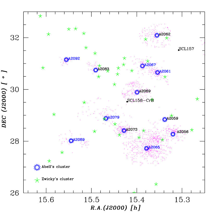
Figure 1: Spatial distribution of the Abell and Zwicky clusters in the CrB-SC core region. The Abell clusters labelled with blue letters belong to the CrB-SC. Also indicated are the positions of the SCL168 (CrB) and SCL157 supercluster centres, as reported by Einasto et al. (2001). Red dots indicate the positions of the galaxies at redshifts within $\pm 0.02$ of the supercluster redshift and inside the optical radius of each Abell cluster. (The redshifts and the optical radius are taken from the NASA Extragalactic Database.)

The first dynamical study of the CrB-SC was carried out by Postman, Geller, & Huchra (1988), through the study of a sample of 1555 galaxies in the vicinity of Abell clusters. They report 97 new redshift measurements over the previous 85. They conclude that the masses of all clusters in the core of the CrB-SC lie in the range $1.5-8.9~{}\times~{}10^{14}~{}M_{\odot}$, while the mass of the SC is approximately $\approx 8.2~{}\times~{}10^{15}~{}M_{\odot}$, which is probably enough to bind the system. They proved also that the dynamical timescales are comparable with the Hubble time, making it unlikely that the system could be virialised, as one might expect. This work was extended by Small, Ma, Sargent, & Hamilton (1998) by increasing the number of galaxies with known redshifts to 528. They quote a value for the mass of the supercluster of $3-8~{}\times~{}10^{16}\ h^{-1}~{}M_{\odot}$, a value slightly higher than the previous one. This is because Postman, Geller, & Huchra (1988) made the assumption that the mass-to-light ratio in the CrB-SC is the same as in the richest Abell clusters and they used a supercluster volume three times smaller. They remark that almost one third of the galaxies in the region are not linked to any Abell cluster, and also emphasize the great contribution to the projected surface density of galaxies of the background cluster A2069 and its surrounding galaxies, located at a redshift $z~{}\approx 0.11$, suggesting the existence of the so-called “A2069 supercluster”. On the other hand, Marini et al. (2004) have analysed on the BeppoSax X-ray data in a search for evidence of a merging signature between the pairs of clusters candidates in the region of CrB-SC A2061-A2067 and A2122-A2124. They find no clear evidence of interaction but detect a candidate shock inside A2061.

Table 1: Clusters: basic data. The coordinates are the optical centre of each cluster. The last two columns show the predicted flux which would be observed by the VSA for those clusters with X-ray measurements (labelled “pred”, see Section 4.1 for details), and the measured value in our final maps (labelled “VSA”). The error bars contain the thermal noise ($\sigma_{n}$), the average primordial CMB (which has been computed to be $\sigma_{CMB}\approx 19$ mJy/beam) and the residual sources ($\sigma_{sour}\approx 6$ mJy/beam) added in quadrature.

Cluster	RA(a)	DEC(a)	z(a)	$L_{x}$(0.1-2.4 keV)	$T_{e}$	$\Delta S_{\nu}^{pred}$	$\Delta S_{\nu}^{VSA}$
	(J2000)	(J2000)		($10^{44}~{}h_{50}^{-2}~{}ergs^{-1}$)	(keV)	(mJy/beam)	(mJy/beam)
A2019	15 02 57.2	+27 11 17	0.0807				$-2.6\pm 24.5$
A2061	15 21 15.3	+30 39 17	0.0784	$3.95^{(b)}$	$5.6^{(b)}$	$-54.7$	$-53.8\pm 27.4$
A2065	15 22 42.6	+27 43 21	0.0726	$4.94^{(b)}$	$8.4^{(b)}$	$-61.7$	$-42.8\pm 23.4$
A2067	15 23 14.8	+30 54 23	0.0739	$0.86^{(c)}$	$3.1^{(c)}$	$-27.7$	$-26.5\pm 27.4$
SCL-158	15 25 16.2	+29 31 30
A2079	15 28 04.7	+28 52 40	0.0690				$-6.7\pm 22.6$
A2089	15 32 41.3	+28 00 56	0.0731				$-28.9\pm 27.9$
A2092	15 33 19.4	+31 08 58	0.0669				$-21.0\pm 28.5$
A2124	15 44 59.3	+36 03 40	0.0656	$1.35^{(b)}$	$3.7^{(b)}$	$-44.3$	$-19.4\pm 29.2$
A2069	15 23 57.9	+29 53 26	0.1160	$8.92^{(b)}$	$7.9^{(b)}$	$-57.1$	$-15.2\pm 27.4$
A2073	15 25 41.5	+28 24 32	0.1717	$3.74^{(c)}$	$5.6^{(c)}$	$-29.9$	$-33.4\pm 22.6$

Notes: (a) NASA Extragalactic Database, (b) Ebeling et al. (1998), (c) Ebeling et al. (2000).

Note the use of $h_{50}=H_{0}/50~{}km~{}s^{-1}Mpc^{-1}$.

3 Observations and data reduction

3.1 Observations with the VSA interferometer

The Very Small Array (VSA) is a 14-element heterodyne interferometric array, tunable between 26 and 36 GHz with a 1.5 GHz bandwidth and a system temperature of approximately 35 K. It is located at an altitude of 2400 m at the Teide Observatory in Tenerife. For this study, the observing frequency was set at 33 GHz, and we used the extended configuration, which uses conical corrugated horn antennae with 322 mm apertures, and has a primary beam FWHM of $2.1\degr$, and a synthesised beam FWHM $\approx 11$ arcmin at the observing frequency. For a detailed description of the instrument see e.g. Watson et al. (2003).

Situated next to the main array is a two-element interferometer, which consists of two 3.7-m diameter dishes with a north–south baseline of 9 m, giving a resolution of $4$ arcmin in a $9$ arcmin field. This interferometer is used for source subtraction (SS), monitoring radio sources simultaneously with the main array observations, as described in Taylor et al. (2003). This strategy neatly copes with the additional problem of source variability.

The observations were carried out during the period spring 2003 – summer 2004, although most of the data were taken in the first months, while the last months were used only to improve the noise levels in those fields with a poorer signal to noise, and to obtain a better measurement of the fluxes of some of the radio sources. Initially, we observed five individual patches covering the interesting central regions of the supercluster, plus two additional pointings separate from the main mosaic and centred on clusters A2019 and A2124. We later added four more pointings to improve the coverage of the supercluster core. These observations are described in Table 2. Each daily observation was approximately four hours in duration. We dedicated between 5 (for CrB-D and CrB-G) and 37 (for CrB-H) days to each pointing. We quote both total observation and integration times, the latter indicating the data retained after flagging (for instance, periods of bad weather).

Table 2: Summary of the observations with the VSA. We list the central coordinate of the eleven pointings, the total observation time, the integration time and the thermal noise achieved for each map (computed from the map far away from the primary beam).

Pointing	RA (J2000)	DEC (J2000)	$\rm T_{obs}$	$\rm T_{int}$	Thermal noise
			(hr)	(hr)	(mJy/beam)
CrB-A	15 23 12.00	+28 06 00.0	54	50	12.4
CrB-B	15 27 48.00	+29 24 00.0	70	70	10.8
CrB-C	15 22 48.00	+30 21 00.0	33	33	18.9
CrB-D	15 32 00.00	+30 45 00.0	19	19	20.5
CrB-E	15 32 00.00	+28 18 00.0	22	22	19.7
CrB-F	15 02 57.20	+27 11 17.3	47	43	14.4
CrB-G	15 45 00.00	+36 03 57.6	19	19	21.4
CrB-H	15 23 00.00	+29 13 30.0	167	130	10.2
CrB-I	15 27 24.00	+30 33 00.0	56	41	18.6
CrB-J	15 32 00.00	+29 31 30.0	55	39	18.9
CrB-K	15 28 00.00	+28 12 00.0	41	33	20.3

3.2 Calibration and data reduction

The primary calibrator for the VSA is Jupiter. The flux scale is transferred to other calibration sources: Tau A (the Crab Nebula) and Cas A, which are observed daily. A detailed description of the VSA calibration process is presented in Watson et al. (2003), whereas in Grainge et al. (2003) and Dickinson et al. (2004) are remarked the specifications adopted for the VSA extended configuration.

In the first VSA studies (e.g. Watson et al. (2003); Grainge et al. (2003)) the calibration scale was based on the effective temperature of Jupiter given by Mason et al. (1999), which extrapolated to $33$ GHz is $T_{Jup}=153\pm 5~{}K$ ($3$% accuracy in temperature). In the most recent VSA published data (Dickinson et al., 2004) we rescale our results using the Jupiter temperature as derived from the WMAP first-year data: $T_{Jup}=146.6\pm 2.0~{}K$ (Page et al., 2003), which agrees with the Mason et al. (1999) value at $1\sigma$ level, but reduces the calibration error from $3$ to $1.5$% in temperature terms ($6$% to $3$% in the power spectrum). In this paper we have also rescaled the Jupiter temperature to the WMAP value, which is the most accurate value published to date.

The correlated signal from each of 91 VSA baselines is processed as described in Watson et al. (2003) and Grainge et al. (2003), and the data checks so described are also applied.

Table 3: List of all the radio sources with measured fluxes at $33$ GHz above $50$ mJy. We quote the extrapolated flux at $33~{}$GHz, and the estimated flux at $33~{}$GHz using the SS observations, which have been used to subtract the sources from the data.

	Name	RA (J2000)	DEC (J2000)	Extrapolated flux	Measured flux by
				NVSS-GB6 at 33 GHz (mJy)	the SS at 33 GHz (mJy)
CrB-F	1459+2708	14 59 39.60	27 8 16.0	83	$132\pm 12$
	1504+2854	15 4 27.30	28 54 25.0	76	$193\pm 14$
	1509+2642	15 9 39.10	26 42 45.0	39	$58\pm 10$
Mosaic	1514+2931	15 14 20.90	29 31 9.0	104	$95\pm 6$
	1514+2855	15 14 40.30	28 55 39.0	72	$63\pm 8$
	1514+2943	15 14 3.70	29 43 21.0	33	$50\pm 13$
	1521+3115	15 21 1.80	31 15 50.0	196	$69\pm 43$
	1522+3144	15 22 9.50	31 44 18.0	243	$296\pm 7$
	1522+2808	15 22 48.90	28 8 51.0	133	$97\pm 5$
	1527+3115	15 27 18.20	31 15 14.0	294	$157\pm 6$
	1528+3157	15 28 52.60	31 57 34.0	75	$98\pm 7$
	1529+3225	15 29 38.70	32 25 23.0	60	$84\pm 38$
	1531+2819	15 31 21.40	28 19 26.0	30	$58\pm 9$
	1532+2919	15 32 20.20	29 19 40.0	71	$51\pm 12$
	1535+3126	15 35 58.90	31 26 25.0	47	$53\pm 5$
	1537+2648	15 37 6.40	26 48 24.0	23	$56\pm 18$
	1539+3103	15 39 15.90	31 3 59.0	107	$86\pm 15$
	1539+2744	15 39 38.80	27 44 33.0	244	$218\pm 10$
CrB-G	1538+3557	15 38 57.40	35 57 9.0	37	$54\pm 12$
	1540+3538	15 40 31.70	35 38 26.0	24	$52\pm 16$
	1544+3713	15 44 44.70	37 13 22.0	25	$50\pm 11$
	1546+3631	15 46 7.60	36 31 7.0	26	$51\pm 18$
	1546+3644	15 46 38.30	36 44 30.0	44	$59\pm 15$
	1547+3518	15 47 51.70	35 18 59.0	87	$77\pm 12$
	1552+3716	15 52 5.30	37 16 5.0	47	$50\pm 18$

3.3 Source subtraction

In order to remove the effect of radio sources from the data, we followed a slightly different approach to that considered for the primordial CMB fields (see Cleary et al. (2004)). For those fields, the Ryle Telescope (RT) was used to identify all the sources above a given threshold at 15 GHz (see Taylor et al. (2003) and Grainge et al. (2003) for the compact and extended arrays, respectively). Using this catalogue, the source subtraction baseline monitored all these sources in real time, and the derived fluxes were subtracted from the VSA main array data. However, for the present study a complete scanning of the region with the RT was not available owing to observing time constraints, so in order to build a source catalogue in the region, we proceeded as follows. All the sources in the NVSS–1.4 GHz (Condon et al., 1998) and GB6–4.85 GHz (Gregory, Scott, Douglas, & Condon, 1996) catalogues closer than $2\degr$ from each pointing position were identified. Using the fluxes from these catalogues, the inferred spectral index between the respective frequencies was used to extrapolate the flux to $33$ GHz. Finally, all sources with predicted fluxes above $20$ mJy at $33$ GHz were monitored using the SS baseline. The flux threshold was chosen according to the requirements for the primordial CMB fields, but, as we shall see below, for the purposes of this paper this limit can be relaxed.

Source positions were assigned according to the coordinates in the GB6 catalogue. This catalogue has a lower angular resolution (FWHM $\approx 3.5$ arcmin) than the NVSS (FWHM $\approx 45$ arcsec), so multiple sources in NVSS could be associated with a single entry in the GB6 catalogue. This was taken into account when computing the spectral index for each source: the adopted flux at the NVSS frequency was derived using the GB6 resolution, combining all sources in NVSS which correspond to a given entry in the GB6 catalogue (i.e. for each GB6 source, we found all the NVSS sources closer than $5$ arcmin, applied the primary beam correction, and summed the corrected fluxes).

Taking into account that the sensitivity of the GB6 catalogue is $18$ mJy at $4.85$ GHz, together with a maximum value of the rising spectral index between $1.4$ GHz and $33$ GHz (e.g. Mason et al. (1999)) of $\alpha=0.5$ ($S\propto\nu^{\alpha}$), we are confident that we have measured all radio sources with fluxes above $\approx 50$ mJy at $33$ GHz. Nevertheless, we appreciate that sources with inverted spectra and higher fluxes may exist, and identify four compact features at the $3\sigma_{n}$ level (being $\sigma_{n}$ the standard deviation of the thermal noise) in our maps of the CrB-SC region. We suspected that these may be radio sources not picked up by our strategy, but source subtractor observations suggest otherwise. No sources with detectable fluxes (i.e. $S>20$ mJy at the 2$\sigma$ level) were found at those positions.

A total of $74$ sources closer than $2\degr$ to any pointing were found to have an extrapolated flux greater than $20~{}$mJy at 33 GHz, and of these, only $25$ had a measured flux with the source subtractor greater than $50~{}$mJy. In Table 3 we present the final list of identified sources with measured fluxes greater than $50$ mJy at $33$ GHz. These values were used to carry out the source subtraction.

It should be noted that this flux limit is larger than that used for the analyses of the primordial CMB fields with the extended VSA array. For that study, we used a flux limit of $20~{}$mJy, which guarantees that the residual contribution from unsubtracted sources is less than the flux sensitivity (Grainge et al., 2003; Dickinson et al., 2004; Cleary et al., 2004), and this could be achieved thanks to the RT survey at $15~{}$GHz. However, as we shall see below (Section $4.2$), the main result of this paper is the detection of two anomalous cold regions with the VSA in the CrB-SC region, that seem difficult to explain as primordial CMB features. We took our list of extrapolated fluxes and used the values to determine the effects on our measurements of the cold spots. We found that the individual effect of any one source was sufficient only to affect our measurements by less than $2$%, and that the collective effect of all sources would cause effects of $1.3$% and $3.2$% in the two spots respectively. This latter error is only twice the calibration error. Thus for the purposes of this paper (in contrast with the VSA power spectrum measurements, where more stringent source constraints were required (Scott et al., 2003; Grainge et al., 2003; Dickinson et al., 2004)), our source subtraction limit of $50~{}$mJy is sufficient.

In any case, an estimate of the confusion noise due to unresolved sources below our source subtraction threshold can be made using the best fit power-law model obtained from the source count above $\approx 50$ mJy (see fluxes in Table 3),

$$n(S)=(17.6\pm 2.3)\left(\frac{S}{70~{}mJy}\right)^{-2.28\pm 0.83}mJy^{-1}sr^{-1}~{}.$$ (1)

Note that this fit has a slope compatible with that of the model presented in Cleary et al. (2004), which was obtained using the source count from the VSA primordial CMB observations. However, the amplitude in our case is a factor $\approx 1.7$ larger. This is as expected since there may be a higher density of radio sources in the supercluster due to the presence of sources associated with the member clusters. Indeed, the model of Cleary et al. (2004) predicts just $15$ radio sources above $50$ mJy in our region of observation, whereas we find $25$. Using the model described by equation 1 we estimate that the residual sources may introduce a confusion noise $\sigma_{sour}=7.3$ mJy/beam. Note however that this result may overestimate the real confusion noise in the regions far away from the CrB-SC clusters, where the source count should be described by the model given in Cleary et al. (2004).

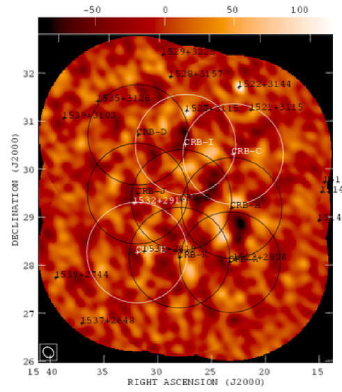
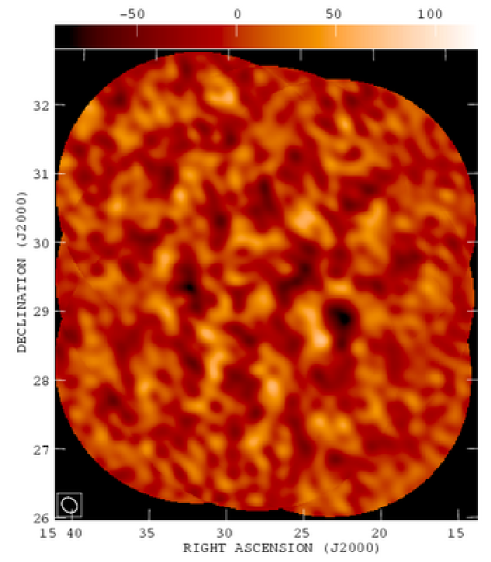
Figure 2: cleaned VSA mosaics built up from pointings CrB-A,B,C,D,E,H,I,J,K. In the un-source-subtracted mosaic (left panel) the circumferences indicate the primary beams FWHM ($2.1\degr$) of the nine pointings, and the crosses the positions of the monitored sources with measured fluxes above $50~{}$mJy. The right panel shows the cleaned source-subtracted mosaic. The synthesised beam FWHM is shown in the bottom left corner ($\approx 11$ arcmin). The noise level is practically uniform across the mosaic at a level $\approx 12$ mJy/beam.

To conclude this section, we also report a problem which was detected during a late stage in the data processing, related to SS measurements. Since the source subtractor continually slews between pointed observations of point sources inside the observed VSA fields, the phase stability of the system has to be checked several times during an observing run, as described in Watson et al. (2003). To this end, we observe several interleaved strong calibration sources close to the considered region on the sky in order to track the phase stability of the system properly. We found that one of the calibration sources used in the CrB-SC central mosaic was not as bright as predicted by the extrapolation and hence was not bright enough to produce a sufficiently accurate determination of the phase. Using Monte Carlo simulations with the known calibrator flux and the sensitivity of the measurement, it is easy to show that a weak calibration source produces an average underestimate of the source flux. From these simulations, we could try to correct all the flux measurements, but this would require us to make an assumption about the variability of each source. Instead, we decided to use a new estimator of the flux of the source that does not require phase calibration.

Let us introduce the estimator $E[S^{2}]=V_{R}^{2}+V_{I}^{2}-2\sigma^{2}$ where $S$ is the flux of the source we are measuring, $V_{R}$ and $V_{I}$ the real and the imaginary parts of the visibility, and $\sigma$ the statistical noise of each measurement. By construction, this estimator is unbiased ($\langle E[S^{2}]\rangle=\langle S^{2}\rangle$) and is not sensitive to phase error of the instrument. If the noise is Gaussian, then $E$ is distributed as a (displaced) $\chi^{2}$ with two degrees of freedom. However, we must note that for our purposes, this estimator can only be used for the case of non-variable sources, because it provides $\langle S^{2}\rangle$ during the whole period of observation, and not $\langle S\rangle$, which is the quantity we are interested in. Thus, we finally decided to use the estimator $E^{\prime}=\sqrt{E}$ to derive the fluxes. This estimator is obviously defined only for positive values of $E$ and in principle is biased to high values of the flux if the signal-to-noise ratio of the measurement is small. This bias was computed and we find that, for the flux sensitivity of the instrument, it is significant only for values of the flux smaller than $50$ mJy. However, we have reduced this bias by averaging the square estimator, $E$, between adjacent measurements of the same source to get a positive value prior to application of the square root. Summarizing, even if we do not have an accurate determination of the phase of the instrument at the time of the observation for some of the sources, their fluxes can be recovered from our measurements using this new estimator, although the error bar on the final measurement will be larger than the one obtained with the standard procedure.

In addition, and as a consistency check, we re-observed the strongest sources in the mosaic, with estimated fluxes above $\approx 60$ mJy, but now using an appropriate calibrator. A variability study was then applied to all these sources following the same criteria as in Cleary et al. (2004), and variable sources were identified. Only five sources were found to be variable. For non-variable sources, the new flux was directly compared to our previous determination to check that our flux values are robust. Final values for the fluxes are presented in Table 3.

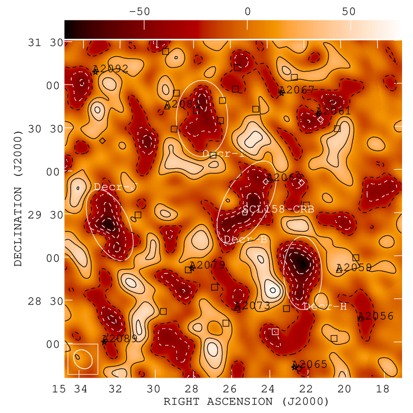
Figure 3: The central region of the cleaned source-subtracted mosaic shown in right panel of Figure 2. We indicate the locations of the four negative decrements. We also show the positions of the clusters extracted from NED. Five-pointed stars are used for the CrB-SC clusters, triangles for the other Abell clusters, squares for the Zwicky clusters, and diamonds for the clusters present in other catalogues. The centre of the supercluster is indicated with a pentagon. Solid contours show positive flux values, while dashed contours show negative flux values, where all contours correspond to $1.5\sigma_{n}$.

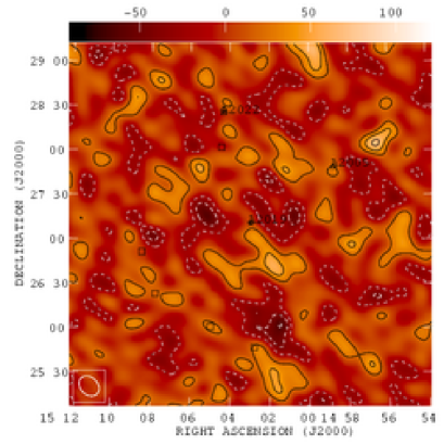
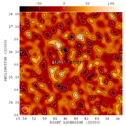
Figure 4: cleaned and source-subtracted VSA maps corresponding to pointings CrB-F (left panel) and CrB-G (right panel). The nomenclature is the same as explained for Figure 3.

3.4 VSA maps

Daily observations are calibrated and reduced as described in Section 3.2 (and references therein) and are held as visibility files, which contain the real and imaginary parts measured at each $uv$-position together with the associated rms noise level. These files are loaded individually into aips (Greisen, 1994), where the map making process is carried out using standard tasks. The individual visibility files are stacked. Each of these stacks contains typically ${\simeq}~{}300\,000$ visibility points, each one averaged over 64 seconds. The source subtraction is implemented in the aperture plane using aips task uvsub, and then the maps for each individual pointing are produced. We used natural weighting, the most appropriate in this case since it produces the highest sensitivity and given that the sampling of the aperture plane is practically uniform. From the nine central pointings we produced the mosaiced map using standard aips tasks. ltess and stess were used to make a map in primary beam-corrected units, followed by a sensitivity map, which is practically uniform around the centre and fails in the outer regions. The two mosaics were divided to give the signal-to-noise, and the result multiplied by the central value of the sensitivity map in order to recover units of mJy/beam. In order to avoid loss of signal to noise in the overlapping regions, and taking into account that the synthesised beams of the nine inner pointings have similar shapes and orientations, the clean mechanism (i.e. the deconvolution of the synthesised beam) has been applied directly to the mosaic, instead of to the individual pointings. To this end, we used the synthesised beam corresponding to the central pointing CrB-B. We placed clean-boxes around the strongest features, and cleaned down to a depth of $2\sigma_{n}$. In the case of the un-source-subtracted mosaics, clean-boxes were also placed around the identified radio sources. The same method was applied to the clean map corresponding to pointing CrB-F. In the case of the CrB-G map, as the signal-to-noise ratio is lower and it is not easy to disentangle the real features from the artefacts, we placed a clean-box around the region encompassing the primary beam FWHM, and clean was applied down to a depth of $3\sigma_{n}$ in this case.

The cleaned mosaics, before and after source subtraction, are shown in Figure 2. In Figure 3 we present a larger scale plot of the regions of interest of the cleaned and source-subtracted mosaic. The maps resulting from the individual pointings CrB-F and CrB-G are shown in Figure 4. The sensitivity values obtained in each individual pointing are shown in Table 2, and the noise level of the overall mosaic is $12$ mJy/beam.

4 Results and discussion

4.1 SZ effect from known clusters in the CrB region

In Table 1 we show the basic data of the eight clusters belonging to the CrB-SC. The X-ray luminosity and electron temperature are given for the four clusters included in the BCS catalogue (Ebeling et al., 1998, 2000); we have also included the more distant clusters A2069 and A2073, for which there are also data in BCS. Since we do not have information on the $\beta$ parameter (which describes the slope of the density profile in a $\beta$-model (Cavaliere & Fusco-Femiano, 1976)) and the core radius from X-rays, we have used the relation given by Hernández-Monteagudo & Rubiño-Martín (2004) in terms of the X-ray luminosity ($L_{x}$),

$$\Delta T_{SZ}^{RJ}=-(0.24\pm 0.06)\left[\frac{L_{x}^{(0.1-2.4~{}keV)}}{10^{44}~{}h_{50}^{-2}erg~{}s^{-1}}\right]^{0.47\pm 0.09}~{}mK$$ (2)

in order to make an estimate of the expected central SZ decrement at the VSA frequency

$$(\Delta T_{SZ})_{0}=-42.545\mu K\left[\frac{T_{e}}{keV}\right]\left[\frac{n_{e0}}{10^{-3}cm^{-3}}\right]\left[\frac{r_{c}}{Mpc}\right]$$

$$\times\int[1+(r/r_{c})^{2}]^{-3\beta/2}d(r/r_{c})~{}~{},$$ (3)

where $T_{e}$ is the electron temperature, $n_{e0}$ the central electron density and $r_{c}$ the core radius.

Making use of the assumption that the inter-cluster (IC) medium is a perfect monoatomic gas in thermal equilibrium, it follows that the temperature is proportional to $M^{\alpha}(1+z)$, with $\alpha=\frac{2}{3}$, while the core radius is proportional to $M^{-\frac{1}{6}}(1+z)^{-\frac{1}{4}}$. Hence, we can obtain a scaling relation of the type $r_{c}=r_{c0}M_{0}^{-\frac{1}{6}}(T_{e}/T_{e0})^{-\frac{1}{4}}$, where $T_{e0}=10^{8}~{}K$, $M_{0}=10^{15}~{}M_{\odot}$, and $r_{c0}=0.13h^{-1}$ Mpc (Markevitch, Forman, Sarazin, & Vikhlinin, 1998). These have been used to obtain a rough estimate of the core radius of each of the clusters for which we have X-ray information. To convert to angular sizes, a cosmology $\Omega_{M}=0.25$, $\Omega_{\Lambda}=0.75$, $h=0.73$, as derived from the last VSA results (Rebolo et al., 2004), was used. Making use of these values, and assuming $\beta=\frac{2}{3}$, we can simulate the response of the VSA to each of these six clusters for which we have X-ray information. The brightness temperature map is converted into flux density, multiplied by the VSA primary beam response, and Fourier transformed to obtain the simulated aperture-plane response of the VSA to the SZ decrement. We must also consider the primary beam attenuation for clusters displaced from the pointing position. The cluster profiles in the aperture plane for the different observing baselines are shown in Figure 5. It is worthwhile comparing this plot with that presented in the VSA SZ work (Lancaster et al., 2004), which shows profiles with a higher amplitude, and similar shapes. Since, in that study, over a selected sample of rich Abell clusters and with similar noise levels, VSA data have shown clear SZ detections in five out of the seven observed clusters, we do not expect a high-significance detection of SZ effect from the single clusters in the CrB-SC region. Moreover, in this case the decrements are affected by the primary beam response, except in clusters A2019 and A2124, in which the pointing centres and cluster coordinates coincide.

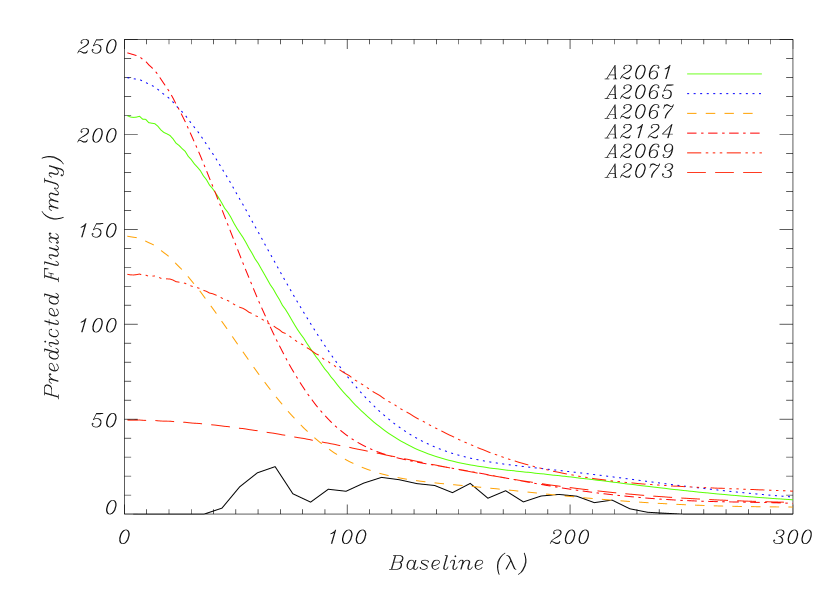
Figure 5: Predicted SZ flux profiles in the aperture plane for four CrB-SC clusters plus other two clusters in the region, as a function of the projected baseline length. The thick solid line represents the VSA weighting function (arbitrary units), computed from these observations.

On the other hand, the simulated visibilities for each cluster, computed as explained above, were convolved with the synthesised beam of the closest observation in order to measure the central flux decrements expected in the maps. These values are shown in Table 1 under the symbol $\Delta S_{\nu}^{\rm pred}$. If we compare the values with the uncertainty in our measurements, we expect to have SZ decrements from single clusters in the region typically with a confidence level between $1$ and $2\sigma$, where $\sigma$ includes now the primordial CMB ($\sigma_{CMB}\approx 19$ mJy/beam), the thermal noise ($\sigma_{n}$) and the residual sources ($\sigma_{sour}\approx 6$ mJy/beam) contributions. This is exactly what we obtain: comparing the cluster flux values from the final maps (see last column in Table 1), we find excellent agreement for those clusters that have a prediction for the flux. In all ten clusters analysed, we get negative flux values, and in the two most luminous clusters in the CrB-SC region, A2061 and A2065, we have $2\sigma$ detections. These two clusters are located close to larger decrements (see Figure 3). Moreover, according to Figure 1 (which includes all galaxies lying within $\pm 0.02$ of the redshift reported in NED for each Abell cluster), A2065 is located in the region with the highest galaxy projected density. We can now combine all these individual measurements to obtain a statistical detection $-24.4\pm 9.2$ mJy/beam ($2.7\sigma$). If we also include in this weighted mean those values from A2069 and A2073, we find $-24.8\pm 8.1$ mJy/beam ($3.0\sigma$), for all the Abell clusters listed in Table 1.

Finally, another point worth noting is the presence of a $5\sigma_{n}$ (signal-to-noise level) decrement (decrement I, see Figure 3) inside pointing CrB-I, located in a region with a large concentration of galaxy clusters, including A2089 and several Zwicky clusters. Their individual SZ effects could have an important contribution to its total decrement.

Table 4: Coordinates, flux densities and temperatures of the two largest decrements found in the mosaic. We quote both the thermal noise ($\sigma_{n}$) and, within parenthesis, the quadrature of the primordial CMB, thermal noise and residual sources ($(\sigma_{cmb}^{2}+\sigma_{n}^{2}+\sigma_{sour}^{2})^{1/2}$) error bars. The last column indicate the percentage over the 5000 simulations with minima under each decrement flux density (within parenthesis, we also show this value when we apply a smoothing to the data; see Section 4.2.1 for details).

	RA (J2000)	DEC(J2000)	$\Delta S_{\nu}$ (mJy/beam)	$\Delta T_{RJ}$ ($\mu$K)	% below $\Delta S_{\nu}$
Decrement B	15 25 21.60	+29 32 40.7	$~{}-70\pm 12~{}(\pm 24)$	$-157\pm 27~{}(\pm 53)$	37.82 (54.16)
Decrement H	15 22 11.47	+28 54 06.2	$-103\pm 10~{}(\pm 22)$	$-230\pm 23~{}(\pm 49)$	0.33 (0.74)

4.2 The origin of the negative spots

The most remarkable feature of the mosaic is the existence of two prominent negative spots, at signal-to-noise levels of $6$ and $10$, situated inside the primary beam FWHM of pointings CrB-B and CrB-H, respectively. Both decrements are extended; indeed they cover an area equivalent to $\approx 3$ VSA synthesised beams. Coordinates, maximum negative flux densities and brightness temperatures of these strong decrements are listed in Table 4. To convert the flux densities into brightness temperatures, we have used the Rayleigh–Jeans expression:

$$T_{RJ}=\frac{\lambda^{2}}{2k_{B}\Omega_{sb}}S~{}~{},$$ (4)

where $\lambda$ is the observing frequency, $k_{B}$ is the Boltzmann constant, and $\Omega_{sb}$ is the solid angle subtended by the synthesised beam.

These decrements are located in regions with no known clusters of galaxies (see Figure 3). Decrement B is located near the centre of the supercluster, and slightly towards the north is the more distant Abell cluster A2069, which Small, Ma, Sargent, & Hamilton (1998) have considered as a possible supercluster because of the large number of galaxies it contains. Decrement I and another negative feature (decrement J) located towards the east of the mosaic, inside pointing CrB-J, have similar flux densities to that of decrement B, but with a lower significance (signal-to-noise of $5$ in both cases). Note that this latter feature is located in the same position as the radio source 1532+2919, so the error bar of its measured flux ($51\pm 12$ mJy, see Table 3), may introduce an additional uncertainty.

We searched for possible negative features in the WMAP maps (Bennett et al., 2003) in the region of the most intense decrement. Given the angular resolution of the VSA extended configuration, we selected the WMAP $W$-band (94 GHz, FWHM=$0.21\degr$) map. From this, we can predict the observed visibilities as seen by the VSA, enabling us to build a “dirty” map. Given the sensitivity of the WMAP map ($\approx 170~{}\mu$K per $7$ arcmin pixel in this region, the corresponding error would be $\approx 108~{}\mu$K in a VSA synthesised beam of $11$ arcmin), we expect to see decrement H only marginally at the $2\sigma_{n}$ level. In the processed $W$-band map we do indeed see a negative spot in the region of decrement H in which the minimum temperature value, $\approx-146\pm 108~{}\mu$K, is located at $15^{h}21^{m}19^{s}+28\degr 55^{\prime}27^{\prime\prime}$ (J2000). Note that although there is an offset of the observed centres of the spots between the VSA and WMAP of $\approx 10$ arcmin, this is consistent with the instrumental resolutions. Given the noise levels involved, we can not conclude anything about the nature of the decrement, i.e. we cannot disentangle at $1\sigma_{n}$ level whether the spectrum between 33 GHz and 94 GHz corresponds to primordial CMB (the decrement should have temperature $-230~{}\mu$K at 94 GHz in this case) or to SZ decrement (in which case the signal should have a temperature $-185~{}\mu$K at 94 GHz).

In principle, decrements B and H, given their sizes and amplitudes, could be either extraordinarily large primordial CMB spots, or SZ signals related to either unknown clusters or to diffuse extended warm/hot gas in the supercluster. It should be noted that only one third of the galaxies in the CrB region are linked to clusters, so SZ contributions could be expected in places where there are no catalogued clusters. As shown in Figures 1 and 3, there are few known galaxies around decrement H, while decrement B is close to a large concentration. This is important since the position of galaxies could trace the warm/hot gas distribution (see, for example, Hernández-Monteagudo et al. (2004)). In the next subsections we explore in detail the three possible explanations for the observed decrements.

4.2.1 CMB anisotropy

In order to quantify the possible contribution from the primordial CMB to these large spots, we carried out Monte-Carlo simulations. Using cmbfast (Seljak & Zaldarriaga, 1996) we generated a CMB power spectrum with a cosmological model defined by the following parameters: $\Omega_{B}=0.044$, $\Omega_{M}=0.25$, $\Omega_{\Lambda}=0.75$, $h=0.73$, $\tau=0.14$, $n_{S}=0.97$, as derived from the most recent VSA results (Rebolo et al., 2004), plus $T_{CMB}=2.725~{}K$, $\Omega_{\nu}=0$ (Bennett et al., 2003), and assuming adiabatic initial conditions. For each decrement we used this power spectrum to carry out 5000 simulations of VSA CMB observations, following the procedure explained in Section 3.3 of Savage et al. (2004), and using the aperture plane coverage from each pointings CrB-B and CrB-H as templates. Each visibility point contains the CMB and thermal noise contributions, plus the confusion level introduced by the residual radio sources below the subtraction threshold of $50$ mJy. Thus $V=V_{cmb}+V_{n}+V_{sour}$, where

$$V_{sour}(\vec{u})=\sum_{i=1}^{ns}{S_{i}e^{2\pi\vec{u}.\vec{x_{i}}}}~{}~{},$$ (5)

where $\vec{u}$ is the position vector of each visibility point, and $S_{i}$ and $\vec{x_{i}}$ the flux and the position vector in the map plane of the i-th source. The fluxes $S_{i}$ are generated using the source count derived from equation 1, yielding a total of $ns=894$ sources distributed between $1$ and $50$ mJy in a region within $2\degr$ of each pointing. The positions $\vec{x_{i}}$ are randomly and uniformly distributed inside this region.

In the last column of Table 4 we quote the percentage of realizations in which the minimum CMB flux value is below that found in the real map in the two cases in question. According to these results the probabilities of decrements B and H being caused by primordial CMB (adding the thermal noise and the residual sources components) are $37.82$% and $0.33$% respectively. Note that here we are considering only the intensity: the angular size of the spots is disregarded. In order to account for this, we have applied Gaussian smoothing (with a FWHM approximately equal to the FWHM of the spots) to both the simulated and the real maps, and in this case the probabilities of the decrements are higher (see also Table 4). Hence, particularly for decrement H, the low probabilities are mainly due to the negative flux density values rather than the corresponding angular sizes.

We calculate the standard deviations of all pixels located within the $2.1\degr$-FWHM of the primary beam in the 5000 realizations, in order to estimate the confusion level introduced by the primordial CMB, the thermal noise and the residual sources components added in quadrature ($\sigma=\sqrt{\sigma_{cmb}^{2}+\sigma_{n}^{2}+\sigma_{sour}^{2}}$, where we have $\sigma_{cmb}\approx 19$ mJy/beam, $\sigma_{n}\approx 11$ mJy/beam and $\sigma_{sour}\approx 6$ mJy/beam). From this, we find that decrements B and H are deviations at $2.95$ and $4.62\sigma$. These results clearly make a primordial CMB fluctuation alone an unlikely explanation for decrement H. We now focus solely on decrement H.

Following Rubiño-Martín & Sunyaev (2003) we performed a fluctuation analysis. In Figure 6 we present a logarithmic plot of the histograms (i.e. the $P(D)$ functions) of pixels values from the 5000 realizations and also using the real data from pointing CrB-H. In the case of the realizations, the $1\sigma$ error bars (containing the primordial CMB, the thermal noise and the residual sources) are displayed. The plot shows a clear excess in the real data compared with the simulations at flux densities below $\sim-30$ mJy/beam, caused by the presence of decrement H. The excess in the positive tail of the curve comes from the two hot spots located towards the north and the east of decrement H in the final mosaic (see Fig. 3). These positive features could be either real hot spots in the sky or artefacts due to the presence of decrement H itself. (Note also that the response of an interferometer has zero mean, so the presence of a strong negative feature in the map could enhance the neighbouring positive spots). It may be that these bright spots are enhanced by the presence of radio sources not identified in the extrapolation. However, these positive features are not present in the map of the region constructed using only VSA baselines $>125\lambda$, suggesting that these structures are extended and not point sources. In order to check if these positive spots are due to the sidelobes introduced by decrement H in the convolution with the synthesised beam, we cleaned the region and find that we obtain lower residuals by placing a clean-box around the negative spot than when the clean-box is placed around the positive spots. Furthermore, with the box around the negative hole, the intensity of the positive spot is reduced by $\approx 12$ %. This is clear evidence that these bright spots are enhanced by the sidelobes of the synthesised beam. Using the cleaned map, the positive tail of the histogram is strongly reduced, while the negative tail is clearly dominant.

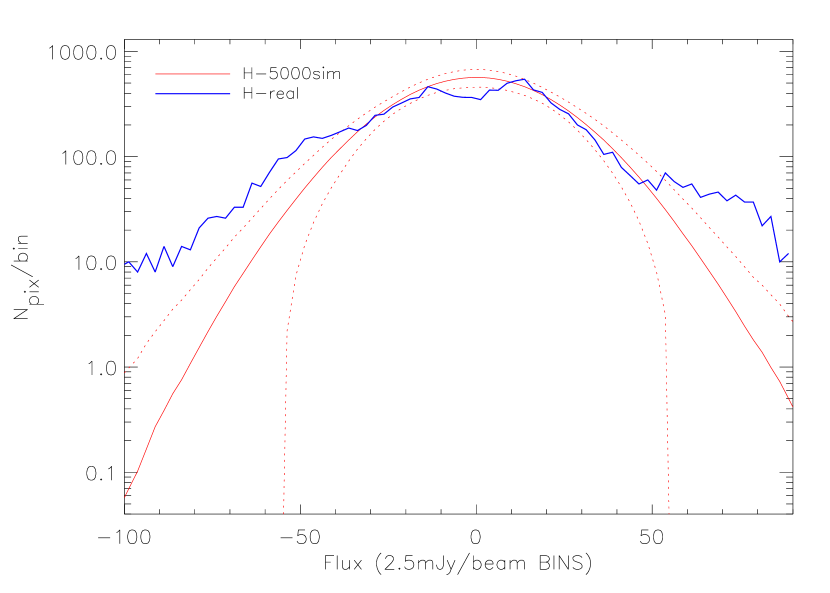
Figure 6: Histograms comparing the distribution of flux densities inside the $2.1\degr$-FWHM of the primary beam in the 5000 simulations (thin curve) and in the real data of pointing CrB-H (thick curve). We also show the $1\sigma$ error bars of the simulations (dotted curve).

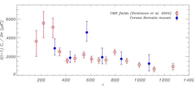
Figure 7: Power spectrum computed from the CrB mosaic, in comparison with that obtained from the most recent VSA observations of primordial CMB fields (Dickinson et al., 2004). The deviation at $\ell\approx 550$ is due to the presence of decrements B and H (see Section 4.2.1 for details).

We also have computed the power spectrum of the mosaic, following the method described in Scott et al. (2003). This is shown in Figure 7, along with that obtained from the most recent primordial CMB observations with the VSA (Dickinson et al., 2004) for comparison. The comparison shows a $2.3\sigma$ deviation from the pure primordial CMB behaviour at $\ell\approx 550$. This is as expected, since this scale corresponds to the size of the large decrements. Indeed, we find that when we compute the power spectrum using data from pointing CrB-H alone, this offset increases to $3.0\sigma$. Moreover, as a consistency check, when we remove pointings CrB-B and CrB-H, which contain decrements B and H, the resulting power spectrum is then compatible with primordial CMB fluctuations on all scales.

4.2.2 SZ effect from clusters of galaxies

In order to explore the possible SZ contribution, we followed the formalism utilized by Holder et al. (2000) (see also Kneissl et al. (2001) and Battye & Weller (2003)) to compute the number of clusters in this region potentially capable of producing a decrement like H. We estimate the mass a cluster would need to have in order to generate an SZ effect at least as intense as a given threshold. In this case the threshold is the amplitude of decrement H, although, to give an idea of the total number of clusters that would be detected in the region, we also considered the confusion level introduced by the quadrature sum of the primordial CMB, the thermal noise and the residual sources ($\sigma\approx 23$ mJy/beam). We then calculate the number of clusters per unit redshift in the Universe with masses above this in a solid angle equal to the entire surveyed region ($\approx 24$ deg²), by using the Press & Schechter (1974) (PS) mass function and also the Sheth & Tormen (1999) (ST) mass function, as this provides a better fit to the simulations (note however that simulations also omit much physics). We have adopted $f_{gas}=0.12$ (Mohr, Mathiesen, & Evrard, 1999) for the gas mass fraction of the cluster, $\delta_{c}=1.69$ (Peebles, 1980) for the critical overdensity, $\sigma_{8}=0.84$ (Bennett et al., 2003) for the spectrum variance in spheres of radius $8$h^-1 Mpc, and the same values as stated above for the other cosmological parameters.

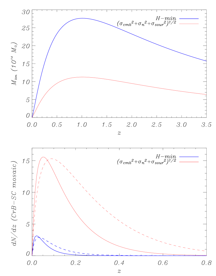
Figure 8: Minimum SZ effect detectable mass versus redshift (top) and number of expected clusters per redshift unit versus redshift (bottom), using as thresholds either the sum in quadrature of the standard deviations of the primordial CMB, the thermal noise and the residual sources (thin curve), and the flux density of spot H (thick curve). The solid and dashed lines correspond respectively to the PS and ST mass functions.

Table 5: Maximum threshold masses, their redshifts, number of detectable clusters in the whole survey, and the most likely redshift for clusters producing a SZ effect larger than either the confusion level introduced by the primordial CMB, the thermal noise and the residual sources and the minimum flux density of pointing H. We have used both the PS and the ST mass functions.

Threshold	Maximum	z where $M_{lim}$	Total number		z where $dN/dz$
	$M_{lim}$ ($10^{14}M_{\odot}$)	is maximum	of clusters		is maximum
			PS	ST	PS	ST
$|$Min-H$|$=$103$ mJy/beam	$27.65$	$1.01$	$0.3$	$0.4$	$0.021$	$0.035$
$\sqrt{\sigma_{cmb}^{2}+\sigma_{n}^{2}+\sigma_{sour}^{2}}$ $\approx$ $23$ mJy/beam	$11.27$	$1.01$	$3.2$	$5.4$	$0.049$	$0.091$

Figure 8 shows the derived threshold mass and the number of clusters per unit redshift versus redshift. By integrating this last curve we obtain the total number of expected clusters in the surveyed region, which is presented in Table 5. The number of SZ clusters that should be detected above the confusion level introduced by the primordial CMB, the thermal noise and the residual sources in the whole surveyed region is $3$ and $5$ respectively for the PS and the ST mass functions. They should be located at mean redshifts $0.049$ or $0.091$, which is close to the mean redshift of the CrB-SC ($\approx 0.07$). Note that in our maps we have detected three clusters in the region above this confusion level (see Table 1). On the other hand, the number of clusters that could produce a decrement at least as intense as H is respectively only $0.3$ or $0.4$ for the PS and the ST prescriptions. Therefore, the probability of decrement H of being caused entirely by a single cluster is very low. However, if we take into account that a decrement such as H due to SZ may be enhanced by the primordial CMB, this probability must be higher. Note finally that these statistics are valid only for a random patch of sky. As we are observing a selected overdense region in the direction of a supercluster, the actual probabilities must be higher. To obtain a more precise result we may turn to N-body simulations, although our analysis is sufficient to get an order of magnitude estimation, and to show that these probabilities are low.

4.2.3 Diffuse extended warm/hot gas

As indicated in Section 1, superclusters may be reservoirs of diffuse warm/hot gas, which in principle might produce a detectable imprint in the low-energy X-ray bands. Zappacosta et al. (2002), and more recently Zappacosta et al. (2004), have claimed an excess of X-ray emission from diffuse structures in a high galactic latitude ROSAT field, and the detection of a significant correlation between the ROSAT-PSPC pointings and the Münster Redshift Survey of galaxies in the Sculptor supercluster region. The SZ effect may provide another tool to detect this gas, thanks to the long path lengths of the photons across these large-scale structures. Using the COBE-DMR data, Molnar & Birkinshaw (1998) were unable to find evidence of an SZ imprint in the region of the Shapley supercluster.

Since decrement B, according to our studies, can be explained through a primordial CMB decrement, we shall focus on decrement H, and explore whether it could have been built up from a concentration of diffuse warm/hot gas ($T_{e}<1~{}keV$). Such a structure producing a detectable SZ effect could also leave an imprint on the less energetic X-ray bands. We have analysed the ROSAT XRT/PSPC All-Sky Survey (Snowden et al., 1997) map, corresponding to the R6 band (0.73–1.56 keV), in order to search for correlated X-ray diffuse emission in the region. The R6 map does not show an excess of emission in the position of the decrement (see Figure 9). The signal in the region of the decrement is $\approx 80-140\times 10^{-6}$ counts/s/arcmin², which comes mainly from the background. In order to perform the ROSAT-VSA correlation, we have adopted two different methods.

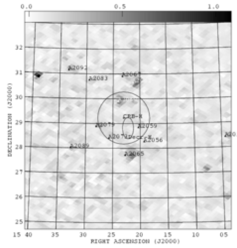
Figure 9: ROSAT–R6 (0.73-1.56 $keV$) (Snowden et al., 1997) map centred on pointing CrB-H. We indicate the positions of all the Abell clusters in the region, emphasizing the CrB-SC clusters with a star. The units indicated in the upper flux bar are $10^{-3}$ counts/s/arcmin². The circle indicate the FWHM of the primary beam of pointing CrB-H, while the ellipse corresponds to the position of decrement H in the VSA mosaic. There is no clear excess of emission in this region.

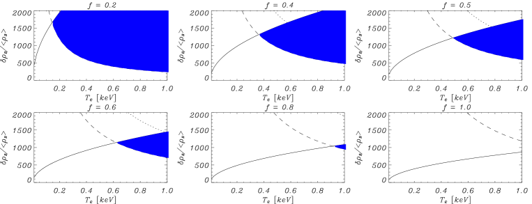
Figure 10: Constraints placed on the overdensity (expressed in terms of baryon density over the mean baryon density) and the electron temperature in the centre of the assumed gas concentration (see Section 4.2.3 for details) that generates decrement H. We take into account that the X-ray emission must be below that in the ROSAT–R6 map (solid line), and that the depth of this structure should be lower than $40$ Mpc (dashed line), or lower than $20$ Mpc (dotted line). Filled regions indicate the acceptable combinations in the parameter space (for $40$ Mpc). The factor f represents the fraction of the decrement that is produced by the SZ effect.

Firstly, we have applied a pixel-to-pixel comparison of the ROSAT-R6 map and the real space cleaned mosaic following the method described in Hernández-Monteagudo & Rubiño-Martín (2004). This method considers the brightness temperature measured by a CMB experiment such as the VSA as the sum of different components: a cosmological signal $T_{CMB}$, the template we want to measure $M$ (in this case, the thermal SZ component traced by ROSAT), instrumental noise $N$, and foreground residuals $F$. The total signal measured at a given position on the sky is then modelled as $T=T_{CMB}+\alpha M+N+F$, where $\alpha$ measures the amplitude of the template induced signal. If all the other components have zero mean and well known correlations functions, and ${\cal C}$ denotes the correlation matrix of the CMB and noise components, then the estimate of $\alpha$ and its statistical error are

$$\alpha=\frac{T{\cal C}^{-1}M^{T}}{M{\cal C}^{-1}M^{T}},\;\;\;\;\sigma_{\alpha}=\sqrt{\frac{1}{M{\cal C}^{-1}M^{T}}}~{}~{}.$$ (6)

The derived value of the correlation between ROSAT and the VSA mosaic is $\alpha=-0.28\pm 0.74~{}\mu K/X$ ($X$ denotes the units of the R6 map, which are counts s^-1 arcmin^-2), which means that there is no significant anticorrelation, as would be expected if it were the case that the decrement is produced by a diffuse gas distribution.

We repeated this analysis but in visibility space, by predicting the expected visibilities from the ROSAT map as seen by the VSA, and performing a similar comparison between the observed and predicted values. In this case, we find $\alpha=-0.21\pm 0.57~{}\mu K/X$ for the CrB-H field. The significance of this value was derived by computing the dispersion of the $\alpha$ value when performing a series of rotations of one map with respect to the other prior to the computation of the predicted visibilities.

Assuming the distance of the supercluster ($\approx 200h^{-1}$ Mpc, derived from the average redshift of the member clusters $\langle z\rangle=0.0725$), the physical transverse size of decrement H is $\approx 2h^{-1}$ Mpc. At typical WHIM electron temperatures , i.e. $T_{e}=0.01~{}keV$ to $T_{e}=1~{}keV$, a homogeneous and spherical gas distribution of this size producing a central SZ decrement of $230~{}\mu$K would have such a high $n_{e}$ that it must have collapsed, with subsequent virialisation. This should also produce detectable X-ray emission, which is not present in the ROSAT-R6 map. In a similar case of a CMB decrement without X-ray emission, Kneissl et al. (1998) discuss various possibilities, but find it difficult to reconcile observations with the process of structure formation. A filament pointing towards us seems in some ways one of the more attractive options. We may therefore consider a larger structure with a lower density so that the path length is long enough to produce a detectable SZ effect ($\Delta T_{SZ}\propto\int n_{e}T_{e}dl$) without significant X-ray emission ($S_{X-ray}\propto\int n_{e}^{2}T_{e}^{1/2}dl$). We can estimate the peak SZ intensity caused by this hypothetical filamentary structure aligned along the line of sight, with a depth $L$, a central electron density $n_{e}$, and electron temperature $T_{e}$, at the VSA frequency of $33$ GHz:

$$\Delta T_{0}f=-21.3~{}\mu K~{}\left[\frac{L}{Mpc}\right]\left[\frac{n_{e}}{10^{-3}cm^{-3}}\right]\left[\frac{T_{e}}{keV}\right]~{}~{}.$$ (7)

Here, $\Delta T_{0}=230~{}\mu$K is the peak SZ decrement. Given that there could also be a contribution from primordial CMB anisotropies, we have introduced the factor $f$ which accounts for the fraction of the decrement due to the SZ effect. For simplicity, we have assumed isothermality and that the electron density is homogeneous along the line of sight. We have assumed that the depth of this structure must be lower than the maximum separation along the line of sight between clusters in the core of the CrB-SC, which is $29h^{-1}$ Mpc = $40$ Mpc. These assumptions set constraints on the overdensity (expressed by the baryon density over the universal mean baryon density) and $T_{e}$ which are represented in Figure 10 by the dashed ($L<40$ Mpc) and the dotted lines ($L<20$ Mpc).

We also require the Bremsstrahlung emission to be low enough that the signal does not leave a detectable imprint on the ROSAT-R6 map. We use equation 7 to derive a relation between $L$ and $T_{e}$, and integrate along the line of sight. We consider a background level of $10^{-4}$ counts/s/arcmin² (see Figure 9) as an upper limit for the X-ray emission in the region of decrement H. Scaling with the signal of the Coma cluster in the same band ($63\times 10^{-4}$ counts/s/arcmin²), we obtain the constraint represented by the solid line of Figure 10. Filled zones in the parameter space show the acceptability regions for structures with lengths of less than $40$ Mpc. These plots show that for $f=1$ there is no reasonable combination of $n_{e}$ and $T_{e}$ to explain the whole decrement. Only values of $f\la 0.7$ are able to explain the decrement. For instance, a filament with a temperature $T_{e}\approx 0.7$ keV, a depth $L\approx 40$ Mpc, and a baryon overdensity $\delta\rho_{B}/\langle\rho_{B}\rangle\approx 850$ would produce a X-ray signal of $\approx 0.6\times 10^{-4}$ counts/s/arcmin², which is almost a factor $2$ below the background confusion level of the ROSAT-R6 map. A structure having these parameters would also produce a peak SZ effect of $\approx 115~{}\mu$K, which is half of the amplitude of the decrement ($f=0.5$). Also, a remarkable alignment is required to achieve this fraction of brightness contrast.

If instead of the value $\delta\rho_{B}/\langle\rho_{B}\rangle\approx 850$, which is computed for the centre of the filament, we assume an average value of $\delta\rho_{B}/\langle\rho_{B}\rangle\approx 450$ over the entire structure, and a $2\times 2$ Mpc² square for the transverse shape of the filament, the total gas mass enclosed in it would be $M_{gas}\approx 5\times 10^{14}M_{\odot}$. This overdensity appears to be difficult to explain in the light of current hydrodynamical galaxy formation simulations, which predict overdensities $\approx 10$ times lower for these large-scale structures (Cen & Ostriker, 1999). If we assume that the dark matter is well traced by the baryonic matter, this leads to an overdensity of $\approx 110$ in terms of the total matter, in contrast to the typical values for non-bound supercluster scales with $\delta\rho/\rho_{c}\sim 5-40$, for structures that have just become virialised with $\delta\rho/\rho_{c}\sim 200$, or inside the typical Abell clusters with $\delta\rho/\rho_{c}\sim 1000$. We note that the derived gas mass contained in this hypothetical filament is comparable to the total baryonic mass in the known CrB-SC clusters, and would represent $\approx 10$% of the total baryonic mass of the supercluster.

5 CONCLUSIONS

We have selected the wholly unusual Corona Borealis supercluster region for CMB observations with the VSA extended array at $33$ GHz. The structures detected in the mosaiced map of the core of the supercluster have significant contributions from primordial CMB anisotropies. However, these maps show negative flux values at the positions of the ten richest clusters in the region, and the two most X-ray luminous CrB-SC clusters, A2061 and A2065, each produce $2\sigma$ decrements. When we combine the flux values from the positions of the CrB-SC member clusters, we obtain a statistical SZ detection with a significance of $2.7\sigma$ ($24.4\pm 9.2$ mJy/beam). If the clusters A2069 and A2073, which have higher redshifts, are added to the sample, we obtain $3.0\sigma$ ($24.8\pm 8.1$ mJy/beam). In addition to this, the mosaic shows, in a region with a high density of Zwicky clusters, a large negative feature, at a signal-to-noise ratio of 5, which could be enhanced by the SZ effects generated by these single clusters.

This mosaic shows two strong and extended negative features with flux densities $-70\pm 12$ mJy/beam ($-157\pm 27~{}\mu$K), and $-103\pm 10$ mJy/beam ($-230\pm 23~{}\mu$K), and positions $15^{h}25^{m}21.60^{s}+29\degr 32^{\prime}40.7^{\prime\prime}$ (J2000) and $15^{h}22^{m}11.47^{s}+28\degr 54^{\prime}06.2^{\prime\prime}$ (J2000), respectively. These decrements are located at positions where there are no known clusters. The first one is placed near the reported centre of the supercluster. In order to disentangle their origins, we have considered the possibility of large primordial CMB fluctuations, or SZ signals related to either unknown clusters or to diffuse extended warm/hot gas in the intergalactic medium of the supercluster. The primordial contribution has been explored by performing simulations of primordial CMB observations with the VSA. These have shown that the size and intensity of decrement B are consistent with primordial CMB fluctuations, whereas in the case of decrement H the probability is only $0.33$%. Decrement H is marginally detected in the W-band map of the WMAP’s first-year dataset, but the current sensitivity does not allow us to disentangle the spectral behaviour of this decrement.

In order to investigate the second possibility we have predicted the number of clusters capable of producing a decrement such as H. To this end we used the Press-Schecter (PS) and also the improved Sheth-Tormen (ST) prescriptions to describe the density of collapsed objects in the Universe. This study showed that the number of random clusters in the VSA observed fields massive enough to produce this feature is 0.3 and 0.4 respectively for the PS and the ST formalisms. Note that this probability has been computed assuming that the whole decrement is due to the SZ effect. If we take into account that there could be a primordial CMB contribution, this probability becomes higher.

The ROSAT-R6 data show no evidence of X-ray emission in the region of decrement H. This fact sets constraints on the electron density and temperature that could have a hypothetical intercluster warm/hot gas distribution capable of producing a decrement as deep as H. If it were in a small volume, then the electron density would be high enough to produce detectable X-ray emission in the typical ranges of WHIM temperatures ($0.01-1$ keV). Hence, we hypothesise that the decrement could be caused by a large filament aligned in the direction of our line of sight. We have explored the possibility that only some fraction of the spot is due to an SZ effect, the primordial CMB being responsible for the rest. In this case, a filament with a length below the size of the supercluster, i.e. $\la 40$ Mpc, a temperature of $0.5-0.8$ keV, and a baryon density in its centre between $500$ and $900$ times the mean baryon density in the local Universe, produces a SZ effect close to one half the central flux density of the decrement, and its X-ray emission would be low and obscured by the background in the ROSAT-R6 map. It would contain a gas mass of $\sim 5\times 10^{14}M_{\odot}$, which is comparable to the total baryonic mass contained in the CrB-SC member clusters. If the value $3\times 10^{16}M_{\odot}$ is assumed for the total mass of the supercluster, this filament would hold the $\sim 10$% of the total expected baryonic mass of the supercluster. However, the required overdensity of such structure is $\sim 10$ times higher than the predictions from N-body galaxy formation simulations for these large-scale filaments. But we stress that: i) we are observing at a very atypical region, and ii) N-body simulations need more physics.

In summary, we are confident that our measurements do show excess decrement, and to explain decrement H we require a combination of primordial CMB fluctuations with either an SZ effect from an unknown cluster or from a large-scale filamentary structure, which would hold a significant fraction of the total baryonic mass of the supercluster. It is worthwhile to carry out multi-frequency observations of decrement H in order to disentangle these possibilities.

References

- Abell (1958) Abell, G. O. 1958, ApJS, 3, 211
- Banday et al. (1996) Banday, A. J., Gorski, K. M., Bennett, C. L., Hinshaw, G., Kogut, A., & Smoot, G. F. 1996, ApJ, 468, L85
- Battye & Weller (2003) Battye, R. A., & Weller, J. 2003, Phys.Rev.D, 68, 083506
- Bennett et al. (2003) Bennett, C. L. et al. 2003, ApJS, 148, 1
- Birkinshaw (1999) Birkinshaw, M., 1999 , Phys Rep , 310 , 97
- Briel & Henry (1995) Briel, U. G. & Henry, J. P. 1995, A&A, 302, L9
- Burles, Nollett, & Turner (2001) Burles, S., Nollett, K. M., & Turner, M. S. 2001, ApJ, 552, L1
- Cavaliere & Fusco-Femiano (1976) Cavaliere, A., & Fusco-Femiano, R. 1976, A&A, 49, 137 S. M., Press, W. H., & Turner, E. L. 1992, ARA&A, 30, 499
- Cen & Ostriker (1999) Cen, R. & Ostriker, J. P. 1999, ApJ, 514, 1
- Cleary et al. (2004) Cleary, K. A., et al. 2004, astro-ph/0412605. Submitted for publication in MNRAS
- Condon et al. (1998) Condon, J. J., Cotton, W. D., Greisen, E. W., Yin, Q. F., Perley, R. A., Taylor, G. B., & Broderick, J. J. 1998, AJ, 115, 1693
- Davé et al. (2001) Davé, R., et al. 2001, ApJ, 552, 473
- Dickinson et al. (2004) Dickinson, C., et al. 2004, MNRAS, 353, 732
- Ebeling et al. (1998) Ebeling, H., Edge, A. C., Bohringer, H., Allen, S. W., Crawford, C. S., Fabian, A. C., Voges, W., & Huchra, J. P. 1998, MNRAS, 301, 881
- Ebeling et al. (2000) Ebeling, H., Edge, A. C., Allen, S. W., Crawford, C. S., Fabian, A. C., & Huchra, J. P. 2000, MNRAS, 318, 333
- Einasto et al. (2001) Einasto, M., Einasto, J., Tago, E., Müller, V., & Andernach, H. 2001, AJ, 122, 2222
- Finoguenov, Briel, & Henry (2003) Finoguenov, A., Briel, U. G., & Henry, J. P. 2003, A&A, 410, 777
- Fosalba, Gaztañaga, & Castander (2003) Fosalba, P., Gaztañaga, E., & Castander, F. J. 2003, ApJ, 597, L89
- Fukugita, Hogan, & Peebles (1998) Fukugita, M., Hogan, C. J., & Peebles, P. J. E. 1998, ApJ, 503, 518
- Grainge et al. (2003) Grainge, K., et al. 2003, MNRAS, 341, L23
- Gregory, Scott, Douglas, & Condon (1996) Gregory, P. C., Scott, W. K., Douglas, K., & Condon, J. J. 1996, ApJS, 103, 427
- Greisen (1994) Greisen E., ed., 1994, AIPS Cookbook. NRAO, Green Bank, WV
- Hernández-Monteagudo & Rubiño-Martín (2004) Hernández-Monteagudo, C. & Rubiño-Martín, J. A. 2004, MNRAS, 347, 403
- Hernández-Monteagudo et al. (2004) Hernández-Monteagudo, C., Genova-Santos, R., & Atrio-Barandela, F. 2004, ApJ, 613, L89
- Holder et al. (2000) Holder, G. P., Mohr, J. J., Carlstrom, J. E., Evrard, A. E., & Leitch, E. M. 2000, ApJ, 544, 629
- Kneissl et al. (1998) Kneissl, R., Sunyaev, R. A., & White, S. D. M. 1998, MNRAS, 297, L29
- Kneissl et al. (2001) Kneissl, R., Jones, M. E., Saunders, R., Eke, V. R., Lasenby, A. N., Grainge, K., & Cotter, G. 2001, MNRAS, 328, 783
- Lancaster et al. (2004) Lancaster, K., et al. 2004, astro-ph/0405582. Accepted for publication in MNRAS
- Markevitch, Forman, Sarazin, & Vikhlinin (1998) Markevitch, M., Forman, W. R., Sarazin, C. L., & Vikhlinin, A. 1998, ApJ, 503, 77
- Mason et al. (1999) Mason, B. S., Leitch, E. M., Myers, S. T., Cartwright, J. K., & Readhead, A. C. S. 1999, AJ, 118, 2908
- Marini et al. (2004) Marini, F., et al. 2004, MNRAS, 353, 1219
- Mohr, Mathiesen, & Evrard (1999) Mohr, J. J., Mathiesen, B., & Evrard, A. E. 1999, ApJ, 517, 627
- Molnar & Birkinshaw (1998) Molnar, S. M., & Birkinshaw, M. 1998, ApJ, 497, 1
- Myers et al. (2004) Myers, A. D., Shanks, T., Outram, P. J., Frith, W. J., & Wolfendale, A. W. 2004, MNRAS, 347, L67
- Page et al. (2003) Page, L., et al. 2003, ApJS, 148, 233
- Peebles (1980) Peebles, P. 1980, The Large-Scale Structure of the Universe (Princeton: Princeton Univ. Press)
- Postman, Geller, & Huchra (1988) Postman, M., Geller, M. J., & Huchra, J. P. 1988, AJ, 95, 267
- Press & Schechter (1974) Press, W. H. & Schechter, P. 1974, ApJ, 187, 425 (PS)
- Rauch et al. (1997) Rauch, M., et al. 1997, ApJ, 489, 7
- Rebolo et al. (2004) Rebolo, R., et al. 2004, MNRAS, 353, 747
- Rubiño-Martín & Sunyaev (2003) Rubiño-Martín, J. A. & Sunyaev, R. A. 2003, MNRAS, 344, 1155
- Savage et al. (2004) Savage, R., et al. 2004, MNRAS, 349, 973
- Scharf et al. (2000) Scharf, C., Donahue, M., Voit, G. M., Rosati, P., & Postman, M. 2000, ApJ, 528, L73
- Scott et al. (2003) Scott, P. F., et al. 2003, MNRAS, 341, 1076
- Seljak & Zaldarriaga (1996) Seljak, U. & Zaldarriaga, M. 1996, ApJ, 469, 437
- Shane & Wirtanen (1954) Shane, C. D. & Wirtanen, C. A. 1954, AJ, 59, 285
- Sheth & Tormen (1999) Sheth, R. K. & Tormen, G. 1999, MNRAS, 308, 126 (ST)
- Small, Sargent, & Hamilton (1997) Small, T. A., Sargent, W. L. W., & Hamilton, D. 1997, ApJS, 111, 1
- Small, Ma, Sargent, & Hamilton (1998) Small, T. A., Ma, C., Sargent, W. L. W., & Hamilton, D. 1998, ApJ, 492, 45
- Snowden et al. (1997) Snowden, S. L., et al. 1997, ApJ, 485, 125
- Sołtan, Freyberg, & Hasinger (2002) Sołtan, A. M., Freyberg, M. J., & Hasinger, G. 2002, A&A, 395, 475
- Spergel et al. (2003) Spergel, D. N., et al. 2003, ApJS, 148, 175
- Taylor et al. (2003) Taylor, A. C., et al. 2003, MNRAS, 341, 1066
- Tittley & Henriksen (2001) Tittley, E. R. & Henriksen, M. 2001, ApJ, 563, 673
- Watson et al. (2003) Watson, R. A., et al. 2003, MNRAS, 341, 1057
- Zappacosta et al. (2002) Zappacosta, L., Mannucci, F., Maiolino, R., Gilli, R., Ferrara, A., Finoguenov, A., Nagar, N. M., & Axon, D. J. 2002, A&A, 394, 7
- Zappacosta et al. (2004) Zappacosta, L., Maiolino, R., Mannucci, F., Gilli, R., Schuecker, P., 2004, astro-ph/0402575. Accepted for publication in MNRAS