O stars with weak winds: the Galactic case

We study the stellar and wind properties of a sample of Galactic O dwarfs to track the conditions under which weak winds (i.e mass loss rates lower than $\sim 10^{-8}$ M_⊙ yr^-1) appear. The sample is composed of low and high luminosity dwarfs including Vz stars and stars known to display qualitatively weak winds. Atmosphere models including non-LTE treatment, spherical expansion and line blanketing are computed with the code CMFGEN (Hillier & Miller hm98 (1998)). Both UV and H$\alpha$ lines are used to derive wind properties while optical H and He lines give the stellar parameters. We find that the stars of our sample are usually 1 to 4 Myr old. Mass loss rates of all stars are found to be lower than expected from the hydrodynamical predictions of Vink et al. (vink01 (2001)). For stars with $\log\frac{L}{L_{\odot}}\ga 5.2$, the reduction is by less than a factor 5 and is mainly due to the inclusion of clumping in the models. For stars with $\log\frac{L}{L_{\odot}}\la 5.2$ the reduction can be as high as a factor 100. The inclusion of X-ray emission (possibly due to magnetic mechanisms) in models with low density is crucial to derive accurate mass loss rates from UV lines, while it is found to be unimportant for high density winds. The modified wind momentum - luminosity relation shows a significant change of slope around this transition luminosity. Terminal velocities of low luminosity stars are also found to be low. Both mass loss rates and terminal velocities of low $L$ stars are consistent with a reduced line force parameter $\alpha$. However, the physical reason for such a reduction is still not clear although the finding of weak winds in Galactic stars excludes the role of a reduced metallicity. There may be a link between an early evolutionary state and a weak wind, but this has to be confirmed by further studies of Vz stars. X-rays, through the change in the ionisation structure they imply, may be at the origin of a reduction of the radiative acceleration, leading to lower mass loss rates. A better understanding of the origin of X-rays is of crucial importance for the study of the physics of weak winds

1 Introduction

Massive stars are known to develop winds so intense that mass loss rate turns out to be the main factor governing their evolution (e.g. Chiosi & Maeder cm86 (1986)). The mechanism responsible for such strong outflows was first pointed out by Milne (milne (1926)) when observations of winds were not yet available: the radiative acceleration in these bright objects was suspected to be large enough to overtake gravitational acceleration, creating expanding atmospheres. The first quantitative description of this process was given by Lucy & Solomon (ls71 (1971)) who computed mass loss rates due to radiative acceleration through strong UV resonance lines. Castor, Abbott & Klein (cak (1975)) made a significant improvement in the understanding of winds of massive stars in their detailed calculation of radiative acceleration including an ensemble of lines by means of their now famous formalism and found mass loss rates $\sim$ 100 times larger than Lucy & Solomon (ls71 (1971)). The theory of radiation driven winds developed by Castor, Abbott & Klein was further improved by Pauldrach et al. (pauldrach86 (1986)) and Kudritzki et al. (kud89 (1989)) who included the effect of the finite size of the star in the radiative acceleration.

In parallel to theoretical studies, observational constraints on the wind properties of massive stars were obtained. Most methods relied on either the measurement of infrared and radio excess emitted in the wind of such stars (Howarth & Prinja hp89 (1989), Leitherer leith88 (1988), Lamers & Leitherer ll93 (1993)), or on the analysis of UV and optical emission or P-Cygni lines (e.g. Leitherer leith88 (1988), Haser haser (1995), Puls et al. puls96 (1996)). The results confirmed the prediction of the theory that the mass loss rate should scale mainly as a power law of luminosity (e.g. Howarth & Prinja hp89 (1989)) and that the terminal velocities are directly proportional to escape velocities (e.g. Lamers et al. lamers95 (1995)). Another success of the radiation driven wind theory came from the so called modified wind momentum - luminosity relation (hereafter WLR). Kudritzki et al. (kud95 (1995)) showed that the quantity $\dot{M}v_{\infty}\sqrt{R}$ (with $\dot{M}$ the mass loss rate, $v_{\infty}$ the terminal velocity and R the stellar radius) should depend only on luminosity (contrary to $\dot{M}$ which also depends slightly on the star mass) which was soon confirmed by the spectroscopic analysis of O and B stars (Puls et al. puls96 (1996), Kudritzki et al. kud99 (1999)). This finding was quite exciting since once calibrated, the WLR could be used as a distance indicator up to several Mpc (Kudritzki kud98 (1998)). Recent determinations of wind parameters with sophisticated atmosphere codes confirm the good agreement between observational constraints and theoretical predictions for bright O stars, both in term of mass loss rate (for which the most recent predictions are those of Vink et al. vink00 (2000), vink01 (2001)) and WLR (see Herrero, Puls & Najarro hpn02 (2002), Crowther et al. paul02 (2002), Repolust et al. repolust (2004)).

In spite of these encouraging results, the behaviour of the wind properties of O stars with relatively low luminosity seems to be a little more complicated. Martins et al. (2002b , n81 (2004), hereafter paper I) have shown that the stellar components of the star forming region N81 of the SMC are O dwarfs with low luminosities and surprisingly weak winds: the mass loss rates are lower than 10^-8 M_⊙ yr^-1 and the modified wind momenta are nearly 2 orders of magnitude lower than expected from the WLR obtained for bright stars. Bouret et al. (jc03 (2003)) also found low mass loss rates for the faintest of the NGC 346 dwarfs they analysed. Although all stars were in the SMC, we showed in paper I that metallicity may not be the only factor responsible for such a strong reduction of the wind strength. In particular, we showed that a Galactic star - 10 Lac - displayed a similar weak wind. One of the explanations we highlighted was a possible link with the youth of the stars since most of them were (or were suspected to be) Vz stars, i.e. young stars lying close to the ZAMS (Walborn & Parker wp92 (1992)). Another possibility was a break down of the scaling relations (especially the WLR) at low luminosity. This reduction of the wind strength at low luminosities was in fact already mentioned by Chlebowski & Garmany (chleb (1991)) more than a decade ago.

In this paper, we try to investigate more deeply the wind properties of low luminosity Galactic stars. The aim is 1) to see if one can exclude the effect of metallicity to explain the weakness of the winds, 2) to test the hypothesis of the link between the weakness of the wind and the youth of the stars and 3) to quantify the wind properties of faint O stars and the luminosity below which such weak winds are observed. For this, we study a sample of O dwarfs with both low and high luminosities. Stars known to display qualitatively weak winds are included together with stars belonging to the Vz subclass. We selected stars showing weak UV lines usually sensitive to winds (from the IUE atlas of Walborn et al. walbornIUE (1985)) and/or with low mass loss rates from the study of Chlebowski & Garmany (chleb (1991)). We also included Vz stars (N. Walborn, private communication) and bright stars (two in common with the Repolust et al. repolust (2004) sample) to examine the dependence of the wind properties on luminosity. Finally, stars from the young star forming region in the Rosette nebula were included.

The remainder of the paper is organised as follows: In Sect. 2 we give information about the observational data we used; Sect. 3 explains how we derived the stellar and wind parameters; Sect. 4 gives the results for individual stars; Sect. 5 highlights the importance of X-rays and magnetic fields in weak wind stars, while Sect. 6 discusses possible sources of uncertainty; the results are discussed in Sect. 7 and the conclusions are given in Sect. 8.

2 Observations

2.1 Optical

Various sources have been used for the optical spectra of the stars studied here. First, the VLT archive provided UVES spectra for HD 152590, HD 38666 and HD 46202. The instrumental resolution varies between 0.04 Å and 0.1 Å, due to different slit widths. The UVES pipeline was used for the reduction of the data. Second, optical data for HD 34078 and HD 15629 were retrieved from the La Palma archive. Spectra obtained with the instrument ISIS on the WHT were reduced using standard procedures under the ESO/MIDAS environment. The spectral resolution is 0.9 Å. Third, spectra of HD 93204, HD 93250 (EMMI) and HD 15629 (La Palma) were provided by Artemio Herrero and Danny Lennon and have a typical resolution of 0.95 Å. Finally for stars HD 93146, HD 93028, HD 46223 and HD 42088, we used EMMI spectra obtained during the nights of 29, 30 and 31 December 2003 on the ESO/NTT in La Silla, under the program 72.D-0038(A) (PI Martins). These spectra were obtained in the red mode of the instrument and provided the H$\alpha$ profiles. The IRAF package was used for the data reduction. For a few stars, we were left with several spectra of the same wavelength range. In that case, we always chose the spectra with the best resolution. The signal to noise ratio depends on the instrument used but is usually larger than 100 in most lines of interest.

2.2 UV

The IUE archive was used to retrieve the UV spectra of all the stars of this study. Spectra in the range 1150-2000 Å obtained with the Short Wavelength Prime (SWP) camera were selected. The typical instrumental resolution is 0.2 Å and a S/N ratio of the order of 10. The normalisation was made “by eye” and turned out to be somewhat uncertain below 1200 Å.

We also retrieved FUSE spectra when available from the MAST archive. The data are provided already reduced (without binning) and co-added by the CALFUSE pipeline (version 1.8.7), and we simply normalised them by eye. Due to the strong Galactic interstellar absorption, many broad absorption bands form H₂ render the bluest part of the FUSE spectra useless for our purpose (e.g. Pellerin et al. pellerin (2002)). We mostly used the 1100-1180 Å range which has a better signal to noise ratio than the IUE spectra for such wavelengths and extends to shorter wavelengths.

Table 1: Adopted parameters for our program stars. The photomerty comes from Chlebowski & Garmany (chleb (1991)), Hiltner (hiltner (1956)), Howarth & Prinja (hp89 (1989)), Humphreys (humph (1978)), Maíz-Apellániz et al. (MA (2004)), Massey et al. (massey01 (2001)), Nicolet (nicolet (1978)), Puls et al. (puls96 (1996)), Schild et al. (schild (1983)), Walborn et al. (walborn02 (2002)). Distance modulus are taken from DeGioia-Eastwood et al. (degioia (2001)), Humphreys (humph (1978)), Maíz-Apellániz et al. (MA (2004)), Markova et al. (mark04 (2004)), Massey et al. (massey01 (2001)), Mason et al. (mason (1998)) and the Webda database. References to the observing data sets retrieved from archives are also given when available.

HD	ST	V	E(B-V)	DM	MV	FUSE	IUE SWP	optical data
38666	O9.5V	5.15${}^{+0.01}_{-0.01}$	0.05${}^{+0.01}_{-0.01}$	8.63${}^{+0.93}_{-0.63}$	-3.64${}^{+0.60}_{-0.93}$	-	6631	ESO/UVES 65.H-0375
34078	O9.5V	5.99${}^{+0.01}_{-0.04}$	0.54${}^{+0.01}_{-0.02}$	8.25${}^{+0.87}_{-0.62}$	-3.92${}^{+0.69}_{-0.96}$	B063	54036	WHT/ISIS
46202	O9V	8.18${}^{+0.02}_{-0.02}$	0.49${}^{+0.01}_{-0.01}$	10.85${}^{+0.05}_{-0.05}$	-4.19${}^{+0.10}_{-0.10}$	-	8845	INT/IDS
93028	O9V	8.36${}^{+0.01}_{-0.01}$	0.26${}^{+0.01}_{-0.01}$	12.09${}^{+0.37}_{-0.38}$	-4.54${}^{+0.38}_{-0.37}$	A118	5521	ESO/EMMI 72.D-0038
152590	O7.5Vz	8.44${}^{+0.02}_{-0.02}$	0.46${}^{+0.10}_{-0.10}$	10.72${}^{+0.69}_{-0.44}$	-3.71${}^{+0.51}_{-0.74}$	-	16098	ESO/UVES 67.B-0504
93146	O6.5V((f))	8.43${}^{+0.02}_{-0.02}$	0.34${}^{+0.01}_{-0.02}$	12.09${}^{+0.37}_{-0.37}$	-4.70${}^{+0.45}_{-0.45}$	-	11136	ESO/EMMI 72.D-0038
42088	O6.5Vz	7.55${}^{+0.01}_{-0.01}$	0.46${}^{+0.01}_{-0.01}$	11.20${}^{+0.20}_{-0.23}$	-4.66${}^{+0.30}_{-0.33}$	P102	7706	ESO/EMMI 72.D-0038
93204	O5V((f))	8.44${}^{+0.02}_{-0.02}$	0.42${}^{+0.01}_{-0.01}$	12.34${}^{+0.45}_{-0.27}$	-5.20${}^{+0.34}_{-0.38}$	-	7023	INT/IDS
15629	O5V((f))	8.42${}^{+0.01}_{-0.01}$	0.74${}^{+0.01}_{-0.01}$	11.38${}^{+0.30}_{-0.30}$	-5.25${}^{+0.30}_{-0.30}$	-	10754	INT/IDS
46223	O4V((f+))	7.27${}^{+0.05}_{-0.02}$	0.54${}^{+0.01}_{-0.01}$	10.85${}^{+0.05}_{-0.05}$	-5.25${}^{+0.10}_{-0.07}$	-	8844	ESO/EMMI 72.D-0038
93250	O3.5V((f+))	7.38${}^{+0.02}_{-0.02}$	0.48${}^{+0.01}_{-0.01}$	12.34${}^{+0.45}_{-0.27}$	-6.45${}^{+0.29}_{-0.48}$	-	22106	INT/IDS

3 Method

Our main concern is to derive wind parameters (mass loss rates, terminal velocities) and modified wind momenta. However, such determinations require reliable stellar parameters, especially effective temperatures. Indeed, any uncertainty in $T_{\mathrm{eff}}$ can lead to an error on $\dot{M}$. We thus first estimate the stellar parameters using the optical spectra, and then we use the UV range + H$\alpha$ line to determine the wind properties.

3.1 Stellar parameters

The main stellar parameters have been determined from blue optical spectra. As such spectra contain diagnostic lines which are formed just above the photosphere and are not affected by winds, plane-parallel models can be used for a preliminary analysis. Hence, we have taken advantage of the recent grid of TLUSTY spectra (OSTAR2002, Lanz & Hubeny ostar2002 (2002)). This grid covers the log g - $T_{\mathrm{eff}}$ plane for O stars and includes optical synthetic spectra computed with a turbulent velocity of 10 km s^-1. The models include the main ingredients of the modelling of O star atmospheres (especially non-LTE treatment and line-blanketing) except that they do not take the wind into account (see Hubeny & Lanz hl95 (1995) for details).

Our method has been the following:

- $V$ sin$i$ : we adopted the rotational velocities from the literature (mostly Penny penny (1996)) and refined them in the fitting process when possible.

- $T_{\mathrm{eff}}$ : the ratio of He i $\lambda$4471 to He ii $\lambda$4542 equivalent widths gave the spectral type which was used to estimate $T_{\mathrm{eff}}$ from the $T_{\mathrm{eff}}$-scale of Martins et al. (2002a ). Then, TLUSTY spectra with effective temperatures bracketing this value were convolved to take into account the rotational velocity and instrumental resolution, and the resulting spectra were compared to the observed profiles of the He i $\lambda$4471 and He ii $\lambda$4542 lines. The best fit led to the constraint on $T_{\mathrm{eff}}$. As the OSTAR2002 grid has a relatively coarse sampling (2500 K steps), we have often interpolated line profiles of intermediate temperatures. A simple linear interpolation was used. For the stars for which the He i $\lambda$4471 and He ii $\lambda$4542 lines were not available, we used He i $\lambda$5876 and He ii $\lambda$5412 as the main indicators.

Secondary $T_{\mathrm{eff}}$ diagnostic lines such as He i $\lambda$4388, He i $\lambda$4713, He i $\lambda$4920, He i $\lambda$4144, He i $\lambda$5016 and He ii $\lambda$4200 were also used to refine the determination (when available). The uncertainty in $T_{\mathrm{eff}}$ depends on the resolution of the spectra and on the rotational broadening. Indeed, the broader the profile, the lower the precision of the fit of the line. The typical error on $T_{\mathrm{eff}}$ is usually of $\pm$ 2000 K but can be reduced when many optical He lines are available. Note that the errors we give are $2\sigma$ errors (we have $T_{\rm eff}\ -error<T_{\rm eff}\ <T_{\rm eff}\ +error$).

We also checked that our final models including winds computed with CMFGEN fitted correctly the optical lines. It turns out that the agreement between TLUSTY and CMFGEN is very good as already noticed in previous studies (e.g. Bouret et al. jc03 (2003)). The problem recently highlighted by Puls et al. (puls05 (2005)) concerning the weakness of the He I singlet lines between 35000 and 40000 K is in fact related to subtle line blanketing effects and is solved when both the turbulent velocity is reduced (in the computation of the atmospheric structure) and other species (Neon, Argon, Calcium and Nickel) are added into the models (see Sect. 4.5).

- $\log g$ : Fits of the wings of H$\gamma$ led to constraints on $\log g$. Once again, interpolations between the OSTAR2002 spectra were made to improve the determination as the step size of the OSTAR2002 grid is 0.25 in log g. H$\beta$, which behaves similarly to H$\gamma$, was used as a secondary indicator. The typical uncertainty in log g is 0.1 dex.

Once obtained, these parameters have been used to derive $L$, $R$ and $M$:

- Luminosity : with $T_{\mathrm{eff}}$ known, we have estimated a bolometric correction according to

$$BC(T_{\rm eff})=27.66-6.84\times\log T_{\rm eff}$$ (1)

which has been established by Vacca et al. (vacca (1996)). Visual magnitudes together with estimates of the reddening and the distance modulus of the star have then lead to M_V and $L$ from:

$$\log\frac{L}{L_{\odot}}=-0.4(M_{\rm{V}}+BC-M_{\odot})$$ (2)

the error on $T_{\mathrm{eff}}$ leads to a typical error of 0.2 dex on BC. Note that we have recently revised the calibration of bolometric corrections as a function of $T_{\mathrm{eff}}$ (see Martins et al. calib05 (2005)), but it turns out that due to line-blanketing effects, BCs are reduced by only 0.1 dex, which translates to a reduction of $\log L$ by 0.04 dex, which is negligible here given the uncertainty in the distance.

The solar bolometric magnitude was taken as equal to 4.75 (Allen allen (1976)). We want to caution here that for most of the stars of this study, the distance is poorly known (with sometimes a difference of 1 magnitude on the distance modulus between existing determinations). This leads to an important error on the luminosity. As this last parameter is crucial for the calibration of the modified wind momentum - relation, we decided to take the maximum error on $L$ by adopting the lowest (resp. highest) luminosity (derived from the lowest -resp. highest- extinction, distance modulus and bolometric correction) as the boundaries to the range of possible luminosities. The typical error on $L$ is $\sim$ $\pm$ 0.25 dex, and the main source of uncertainty is the distance.

- Radius : Once $T_{\mathrm{eff}}$ and $L$ are known, $R$ is simply derived from

$$R=\sqrt{\frac{L}{4\pi\sigma T_{\rm eff}^{4}}}$$ (3)

where $\sigma$ is the Stefan Boltzmann constant. Standard errors have been derived according to

$$\Delta\log R=0.5\sqrt{(\Delta\log L)^{2}+(4\Delta\log T_{\rm eff})^{2}}$$ (4)

- M : The (spectroscopic) mass is derived from $g$ and $R$ according to

$$M=\frac{gR^{2}}{G}$$ (5)

and the standard error is given by

$$\Delta\log M=\sqrt{(\Delta\log g)^{2}+(2\Delta\log R)^{2}}$$ (6)

With this set of stellar parameters, we have run models including winds to derive the mass loss rate and the terminal velocity (see next section). The stellar parameters giving the best agreement between observations and models with winds were adopted as the final stellar parameters.

3.2 Wind parameters

UV (and FUV when available) spectra and H$\alpha$ profiles were used to constrain the wind parameters. In the case where mass loss rates were low, priority was given to UV indicators since H$\alpha$ becomes insensitive to $\dot{M}$: for such situations, we checked that the H$\alpha$ line given by our models with $\dot{M}$ estimated from UV was consistent with the observed line. We want to stress here that it is only because metals are now included in a reliable way in new generation atmosphere models that such a study is possible. Indeed, UV metallic lines now correctly reproduced allow to push the limits of mass loss determination below $\sim 10^{-8}$ M_⊙ yr^-1.

Models including stellar winds were computed with the code CMFGEN (Hillier & Miller hm98 (1998)). This code allows for a non-LTE treatment of the radiative transfer and statistical equilibrium equations in spherical geometry and includes line blanketing effects through a super-level approach. The temperature structure is computed under the assumption of radiative equilibrium . At present, CMFGEN does not include self-consistently the hydrodynamics of the wind so that the velocity and density structures must be given as input (but hydrodynamical quantities computed from the final atmosphere model are given as output). In order to be as consistent as possible with the optical analysis, we have used TLUSTY structures for the photosphere part and we have connected them to a classical $\beta$ law ($v=v_{\infty}(1-\frac{R_{\star}}{r})^{\beta}$) representing the wind part. We chose $\beta=1.0$ as the default value for our calculation since it turns out to be representative of O dwarfs (e.g. Massa et al. massa03 (2003)). The TLUSTY structures have been taken from the OSTAR2002 grid or have been linearly interpolated from this grid for $T_{\mathrm{eff}}$ not included in OSTAR2002. This method has also been used by Bouret et al. (jc03 (2003)) and has shown good consistency between CMFGEN and TLUSTY photospheric spectra.

Clumping can be included in the wind models by means of a volume filling factor $f$ parameterised as follows: $f=f_{\infty}+(1-f_{\infty})e^{-\frac{v}{v_{\rm init}}}$ where $f_{\infty}$ is the value of $f$ at the top of the atmosphere and $v_{\rm init}$ is the velocity at which clumping appears. As in Bouret et al. (jc03 (2003)), we chose $v_{\rm init}=30$ km s^-1.

A depth independent microturbulent velocity can be included in the computation of the atmospheric structure (i.e. temperature structure + population of individual levels). We chose a value of 20 km s^-1 as the default value in our computations. Several tests (Martins et al. 2002a , Bouret et al. jc03 (2003)) indicate that a reasonable change of this parameter has little effect on the emergent spectrum, except for some specific lines (see Sect. 4.5). For the computation of the detailed spectrum resulting from a formal solution of the radiative transfer equation (i.e. with the populations kept fixed), a depth dependent microturbulent velocity can be adopted. In that case, the microturbulent velocity follows the relation $v_{turb}(r)=v_{min}+(v_{max}-v_{min})\frac{v(r)}{v_{\infty}}$ where $v_{min}$ and $v_{max}$ are the minimum and maximum microturbulent velocities. By default, we chose $v_{min}$ = 5 km s^-1 in the photosphere, and $v_{max}$ = min (0.1 $v_{\infty}$, 200) km s^-1 at the top of the atmosphere. For some stars, we had to increase $v_{min}$ from 5 to 10 km s^-1 to be able to fit correctly the observed spectra.

CMFGEN allow the possibility to include X-ray emission in the models. In some cases (see next Section), we had to include such high energy photons. Practically, as X-rays are thought to be emitted by shocks distributed in the wind, two parameters are adopted to take them into account: one is a shock temperature (chosen to be $3\times 10^{6}$ K since it is typical of high energy photons in O type stars, e.g. Schulz et al. schulz03 (2003), Cohen et al. cohen03 (2003)) to set the wavelength of maximum emission, and the other is a volume filling factor which is used to set the level of emission. With this formalism, X-ray sources are distributed throughout the atmosphere and the emissivities are taken from tables computed by a Raymond & Smith code (Raymond & Smith rs77 (1977)). We include X-rays in the models for the four faintest stars and in test models for the strong lined star HD 93250 as explained in Sect. 5, using measured X-ray fluxes or a canonical value of $L_{\rm X}/L_{\rm bol}=-7.0$.

The main wind parameters we have determined are the mass loss rate ($\dot{M}$) and the terminal velocity (v_∞). Constraints on the amount of clumping were also derived when possible. The terminal velocities have been estimated from the blueward extension of the absorption part of UV P-Cygni profiles which occurs up to $v_{\infty}$ + $v_{max}$ where $v_{max}$ is the maximum microturbulent velocity described above: fits of the UV P-Cygni profiles using the above relation for microturbulent velocity allows a direct determination of $v_{\infty}$. Note that other definitions of the terminal velocity exist (see Prinja, Barlow & Howarth (Prinja90 (1990))).. The typical uncertainty in our determination of $v_{\infty}$ is 200 km s^-1 (depending on the maximum microturbulent velocity we adopt).

Fits of strong UV lines such as N v $\lambda$1240  C iv $\lambda\lambda$1548,1551  Si iv $\lambda\lambda$1394,1403  O v $\lambda$1371 and N iv $\lambda$1718 provide constraints on $\dot{M}$. H$\alpha$ is also sensitive to $\dot{M}$: in dwarfs with weak winds, a quasi photospheric profile is expected but the line can be used to estimate upper limits on the mass loss rate as it is filled by emission when $\dot{M}\gtrsim 10^{-8}$ M_⊙ yr^-1. Also, in the case of weak winds C iv $\lambda\lambda$1548,1551 is actually the only line showing some sensitivity to wind and was in several cases our best $\dot{M}$ estimator. Given this, we tried to adjust the mass loss rate (and clumping parameters) to get the best fit of both the UV wind sensitive lines and H$\alpha$.

As regards the abundances, we have taken as default values the solar determinations of Grevesse & Sauval (gs98 (1998)) since the stars of this study are are all Galactic stars. CNO solar abundances have been recently revised downward by Asplund (asplund04 (2004)). However, we preferred to rely on the Grevesse & Sauval abundances since they have been widely used in previous studies of massive stars and are therefore more suited for comparisons. When necessary, we indicate if these abundances have been changed to get a better fit.

4 Results

In this Section, we present the results of the analysis for each star (from the latest to the earliest type ones) and highlight the main difficulty encountered in the fitting process. The observed properties and adopted parameters are given in Table 1. The derived stellar and wind parameters are gathered in Table 2, while results from previous studies of wind properties are given in Table 3.

Spectra from atmosphere models are convolved to include the instrumental resolution of the observational data and the projected rotational velocity of the star. The wavelength range between $\sim$ 1200 and $\sim$ 1225 Å is not used in the spectral analysis since it suffers from a strong interstellar Lyman absorption.

A general comment concerning effective temperatures is that we find values lower than previous determinations (see table 3) since line-blanketing is included in our models. This effect is now well known and has been highlighted by several studies (Martins et al. 2002a , calib05 (2005), Crowther et al. paul02 (2002), Markova et al. mark04 (2004)). Our mass loss rates are also generally lower than previous determination for reasons discussed in Sect. 7.2.2.

Table 2: Derived stellar and wind parameters of the Galactic stars studied here. The escape velocities were computed from the spectroscopic derived mass, radius and luminosity. The evolutionary masses have been estimated from the isochrones of Lejeune & Schaerer (lejeune (2001)). Projected rotational velocities were adopted from Penny (penny (1996)), Howarth & Prinja (hp89 (1989)), Howarth et al. (howarth97 (1997)) and Villamariz et al. (villamariz02 (2002)) and refined in the fitting process when possible.

HD	38666	34078	46202	93028	152590	93146	42088
$T_{\mathrm{eff}}$(kK)	33$\pm 1$	33$\pm 2$	33$\pm 2$	34$\pm 2$	36$\pm 1$	37$\pm 2$	38$\pm 2$
BC	-3.25${}^{+0.10}_{-0.08}$	-3.25${}^{+0.10}_{-0.08}$	-3.25${}^{+0.10}_{-0.08}$	-3.34${}^{+0.18}_{-0.17}$	-3.52${}^{+0.08}_{-0.08}$	-3.59${}^{+0.13}_{-0.15}$	-3.67${}^{+0.16}_{-0.15}$
log g	4.0$\pm 0.1$	4.05$\pm 0.1$	4.0$\pm 0.1$	4.0$\pm 0.1$	4.10$\pm 0.1$	4.0$\pm 0.1$	4.0$\pm 0.1$
$V$ sin$i$(km s-1)	111	40	30	50	66	80	60
log $\frac{L}{L_{\odot}}$	4.66${}^{+0.40}_{-0.30}$	4.77${}^{+0.41}_{-0.32}$	4.87${}^{+0.07}_{-0.07}$	5.05${}^{+0.22}_{-0.22}$	4.79${}^{+0.33}_{-0.24}$	5.22${}^{+0.23}_{-0.25}$	5.23${}^{+0.19}_{-0.19}$
R (R⊙)	6.58${}^{+3.89}_{-2.45}$	7.47${}^{+4.55}_{-2.83}$	8.38${}^{+0.88}_{-0.81}$	9.71${}^{+3.11}_{-2.38}$	6.42${}^{+3.00}_{-2.05}$	9.97${}^{+3.29}_{-2.49}$	9.56${}^{+2.61}_{-2.07}$
Mspectro (M⊙)	16${}^{+0.25}_{-0.10}$	23${}^{+38}_{-11}$	26${}^{+9}_{-7}$	34${}^{+28}_{-16}$	19${}^{+23}_{-10}$	36${}^{+31}_{-17}$	33${}^{+24}_{-14}$
Mevol (M⊙)	19	20	21	25	22	30	31
vesc (km s-1)	920	1043	1046	1112	1015	1106	1100
$v_{\infty}$(km s-1)	1200	800	1200	1300	1750	2800	1900
$\log$ $\dot{M}$(M⊙ yr-1)	$-$9.5$\pm 0.7$	$-$9.5$\pm 0.7$	$-$8.9$\pm 0.7$	$-$9.0$\pm 0.7$	$-$7.78$\pm 0.7$	$-$7.25$\pm 0.7$	$-$8.0$\pm 0.7$
vturb (km s-1)	5-120	5-80	5-120	5-130	10-175	5-200	5-190
$f_{\infty}$	1.0	1.0	1.0	1.0	1.0	1.0	1.0
$\log\dot{M}_{Vink}$ (M⊙ yr-1)	$-$7.41	$-$7.38	$-$7.23	$-$6.97	$-$7.15	$-$6.58	$-$6.17
$\log\dot{M}v_{\infty}\sqrt{R}$	24.79	24.64	25.44	25.41	26.67	27.50	26.57

Table 2: Continued.

HD	93204	15629	46223	93250
$T_{\mathrm{eff}}$(kK)	40$\pm 2$	41$\pm 2$	41.5$\pm 2$	44$\pm 2$
BC	-3.82${}^{+0.14}_{-0.16}$	-3.89${}^{+0.15}_{-0.15}$	-3.93${}^{+0.15}_{-0.15}$	-4.10${}^{+0.12}_{-0.12}$
log g	4.0$\pm 0.1$	3.75$\pm 0.1$	4.0$\pm 0.1$	4.0$\pm 0.1$
$V$ sin$i$(km s-1)	130	90	130	110
log $\frac{L}{L_{\odot}}$	5.51${}^{+0.25}_{-0.20}$	5.56${}^{+0.18}_{-0.18}$	5.57${}^{+0.09}_{-0.10}$	6.12${}^{+0.25}_{-0.17}$
R (R⊙)	11.91${}^{+4.23}_{-3.14}$	12.01${}^{+3.08}_{-2.47}$	11.86${}^{+1.78}_{-1.58}$	19.87${}^{+6.98}_{-3.87}$
Mspectro (M⊙)	52${}^{+47}_{-25}$	30${}^{+20}_{-12}$	51${}^{+22}_{-16}$	144${}^{+130}_{-56}$
Mevol (M⊙)	41	44	45	105
vesc (km s-1)	1178	799	1157	1461
$v_{\infty}$(km s-1)	2900	2800	2800	3000
$\log$ $\dot{M}$(M⊙ yr-1)	$-$6.75$\pm 0.7$	$-$6.5$\pm 0.7$	$-$6.5$\pm 0.7$	$-$6.25$\pm 0.7$
vturb(km s-1)	5-200	10-200	10-200	10-200
$f_{\infty}$	0.1	0.1	0.1	0.01
$\log\dot{M}_{Vink}$ (M⊙ yr-1)	$-$6.11	$-$5.74	$-$5.97	$-$5.25
$\log\dot{M}v_{\infty}\sqrt{R}$	28.05	28.29	28.28	28.68

Table 3: Comparison between our derived wind parameters ($\dot{M}$, $v_{\infty}$, shown in bold text) and previous determinations. (1) Leitherer (leith88 (1988)), (2) Bernabeu et al. (bernabeu (1989)), (3) Howarth & Prinja (hp89 (1989)), (4) Prinja et al. (Prinja90 (1990)), (5) Chlebowski & Garmany (chleb (1991)), (6) Lamers & Leitherer (ll93 (1993)), (7) Lamers et al. (lamers95 (1995)), (8) Puls et al. (puls96 (1996)), (9) Howarth et al. (howarth97 (1997)), (10) Lamers et al. (lamers99 (1999)), (11) Repolust et al. (repolust (2004)), (12) Markova et al. (mark04 (2004)).

HD	$\log$ $\dot{M}$		$v_{\infty}$
38666	$<$ $-$7.22 (1), $-$7.8 (3)		2000 (1), 1000 (3)
	$-$8.31 (5)
	$-$9.5		1200
34078	$-$6.6 (3)		750 (3)
	$-$9.5		800
46202	$<$ $-$6.87 (1), $-$7.2 (3)		2100 (1), 750 (3)
	$-$8.10 (5)		1150 (5), 1590 (2)
	$-$8.9		1200
93028	$-$7.0 (3)		1500 (3), 1780 (2)
	$-$9.0		1300
152590	$-$6.9 (3), $-$7.36 (5)		2150 (3), 2300 (5)
			1785 (9)
	$-$7.78		1750
93146	$-$6.9 (3)		2975 (3), 3200 (2)
			2565 (4), 2640 (9)
	$-$7.25		2800
42088	$-$6.35 (1), $-$7.0 (3)		2550 (1), 2030 (3)
	$-$6.82 (5), $-$6.42 (12)		2300 (5), 2420 (2)
			2155 (4), 2215 (9)
			2200 (12)
	$-$8.0		1900
93204	$-$6.1 (3)		3250 (3), 3180 (2)
			2890 (4), 2900 (7)
	$-$6.75		2900
15629	$-$5.89 (11)		3200 (11), 3220 (2)
			2810 (9)
	$-$6.5		2800
46223	$-$5.75 (1), $-$5.8 (3)		3100 (1), 3100 (3)
	$-$5.62 (5), $-$5.85 (6)		3100 (5), 2800 (6)
	$-$5.68 (10)		2800 (10), 3140 (2)
			2910 (4), 2900 (7)
	$-$6.5		2800
93250	$-$4.9 (8), $-$4.6 (3)		3250 (8), 3350 (3)
	$-$5.46 (11)		3250 (11), 3470 (2)
			3230 (9)
	$-$6.25		3000

4.1 HD38666

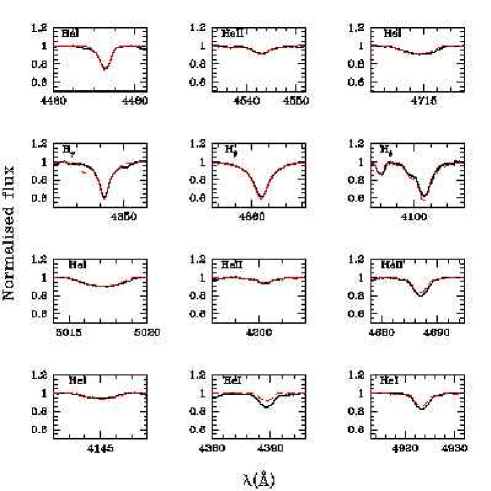
Figure 1: Best fit (red dashed line) of the optical spectrum (black solid line) of HD 38666. The effective temperature is 33000 K, $\log g$ = 4.0 and $V$ sin$i$ = 110 km s^-1.

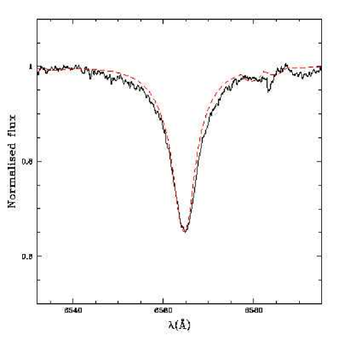
Figure 2: Best fit (red dashed line) of the observed H$\alpha$ line (black solid line) of HD 38666. We have derived $\dot{M}$ = $10^{-9.5}$ M_⊙ yr^-1 and $v_{\infty}$ was 1200 km s^-1.

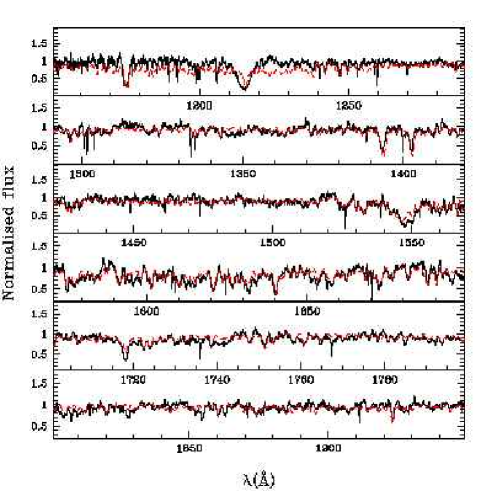
Figure 3: Best fit (red dashed line) of the UV spectrum (black solid line) of HD 38666. For this model, $\dot{M}$ = $10^{-9.5}$ M_⊙ yr^-1, $v_{\infty}$ = 1200 km s^-1 and $\log L_{\rm X}/L_{\rm bol}=-6.87$

HD 38666 (also $\mu$ Col) is an O9.5V runaway star for which we derive an effective temperature of 33000 K from the fit of the optical He lines, as shown in Fig. 1. A value of $\log g=4.0$ is derived from the Balmer lines.

The H$\alpha$ and UV fits are given in Fig. 2 and Fig. 3. The best fits are obtained for $\dot{M}$ = $10^{-9.5}$ M_⊙ yr^-1 and $v_{\infty}$ = 1200 km s^-1. Importantly, X-rays have been included in the modelling with $\log\frac{L_{\rm X}}{L_{\rm bol}}=-6.87$ as indicated by the observed X-ray emission (see Table 4). If this high energy component is not included, we need a mass loss rate 10 times lower to fit the C iv $\lambda\lambda$1548,1551 line. The reason for this is that the ionisation structure of the wind is increased when X-rays are present, leading to a lower C IV ionisation fraction, and thus requiring a higher mass loss rate to reproduce the observed line profile (see Sect. 5 for a more complete discussion). Note that the fit of the C iv $\lambda\lambda$1548,1551 profile is not perfect. This is due to the presence of interstellar absorption which adds to the photospheric component. However, the fit of the blueshifted wind part of the line is good and is not affected by interstellar absorption (see also paper I). Previous estimates of $\dot{M}$ range between $10^{-8.31}$ and $10^{-7.22}$ M_⊙ yr^-1 (see Table 3). Our estimate is lower than all these determinations. The determination of Leitherer (leith88 (1988)) relies only on the H$\alpha$ wind emission, which in the case of low mass rates is very small and difficult to disentangle from the photospheric absorption. The studies of Chlebowski & Garmany (chleb (1991)) and Howarth & Prinja (hp89 (1989)) are based on the fit of UV resonance lines with the following method: the optical depth as a function of the velocity (only for unsaturated profiles) is determined by profile fitting; from this, the determination of the mass loss rate requires the adoption of an ionisation structure which may or may not be representative of the real ionisation in the atmosphere. This assumption may affect the $\dot{M}$ determination.

As for $v_{\infty}$, a higher terminal velocity leads to a too-much-extended blueward absorption in C iv $\lambda\lambda$1548,1551. The value of $v_{\infty}$ we derive is just above the escape velocity. Leitherer (leith88 (1988)) estimated $v_{\infty}$ = 2000 km s^-1  while Howarth & Prinja (hp89 (1989)) found 1000 km s^-1 (see Table 3), illustrating the uncertainty in the exact value of the terminal velocity of HD 38666.

4.2 HD34078

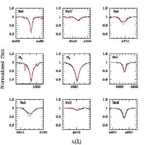
Figure 4: Best fit (red dashed line) of the optical spectrum (black solid line) of HD 34078. Here, $T_{\mathrm{eff}}$ = 33000 K, $\log g$ = 4.05 and $V$ sin$i$ = 40 km s^-1.

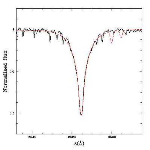
Figure 5: Best fit (red dashed line) of the observed H$\alpha$ line (black solid line) of HD 34078. Here, $\dot{M}$ = $10^{-9.5}$ M_⊙ yr^-1 and $v_{\infty}$ = 800 km s^-1.

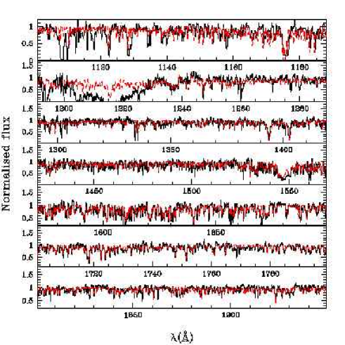
Figure 6: Best fit (red dashed line) of the UV spectrum (black solid line) of HD 34078. The wind parameters are: $\dot{M}$ = $10^{-9.5}$ M_⊙ yr^-1, $v_{\infty}$ = 800 km s^-1 and $\log L_{\rm X}/L_{\rm bol}=-7.0$

HD 34078 (also AE Aur) is a runaway O9.5V star possibly formed as a binary (with $\mu$ Col, see Hoogerwerf et al. hbz01 (2001)) and ejected after a binary - binary interaction with $\iota$ Ori (see Sect. 4.1). Fig. 4 shows the best fit of the optical spectrum. From this best fit model, we derive an effective temperature of 33000 K. This is confirmed by the good fit of the iron lines shown in Fig. 7. Note that the presence of C ii $\lambda\lambda$6578,6582 in the model (see Fig. 5) may indicate a slightly too low effective temperature. Test models reveals that increasing $T_{\mathrm{eff}}$ to 34000 K weakens this doublet. However, since these lines also depends on the C abundance, we prefer to rely on the He lines and UV iron forests estimate. Also, improving the model atom for C ii produces a weaker line since over recombination routes are available, reducing the populations of the C ii $\lambda\lambda$6578,6582 transition levels. This shows that the value for $T_{\mathrm{eff}}$ reported in Table 2 should be considered with its uncertainty of $\pm$ 2000 K. Our modelling indicates that $V$ sin$i$ = 40 km s^-1 seems to better reproduce the observation, especially the optical spectra. The gravity determined by Villamariz et al. (villamariz02 (2002)) gives a good fit of the Balmer lines, so that we adopt $\log g=4.05$ The other stellar parameters are gathered in Table 2.

Figs. 5 and 6 show the fit of the H$\alpha$ line and UV spectrum of HD 34078. As we have shown that X-rays seem to be important for weak winds (see also next stars) and as HD 34078 shows no sign of a strong wind, we have adopted $\log L_{\rm X}/L_{\rm bol}=-7.0$. Indeed, no X-ray measurement exists for HD 34078 and we have thus adopted the classical value for O stars (e.g. Chlebwoski & Garmany chleb (1991)). A reasonable agreement between the two types of mass loss indicators (H$\alpha$ and UV lines) is found for $\dot{M}$= $10^{-9.5}$ M_⊙ yr^-1and a terminal velocity of 800 km s^-1. Again, our value of $\dot{M}$ is lower than previous determinations (see Table 3).

Surprisingly, the derived terminal velocity is similar to or even lower than the escape velocity (1043 km s^-1). However, given the large error on M and R, the escape velocity is also very uncertain. Also, a value of $v_{\infty}$ lower than v_esc is possible since the escape velocity quoted here is the photospheric escape velocity, and a velocity in the wind of the order $v_{\infty}$ is obtained only in the outer atmosphere where the local escape velocity is much lower. Moreover, the weakness of the wind features may actually lead to underestimate of the terminal velocity (see also Sect. 7.2.1).

For HD 34078, we have used the He and CNO abundances of Villamariz et al. (villamariz02 (2002)). They are nearly solar, except for C which is found to have an abundance of $\sim$ 1/2 solar.

Figure 7: Zoom on the Iron line forests from Fig. 6 showing the good agreement between the predicted spectrum (dotted line) and the observed spectrum (solid line) and confirming the $T_{\mathrm{eff}}$ estimate.

4.3 HD46202

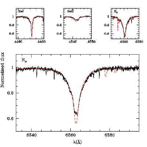
Figure 8: Best fit (red dashed line) of the optical spectrum (black solid line) of HD 46202. Here, $T_{\mathrm{eff}}$ = 33000 K, $\log g$ = 4.0, $V$ sin$i$ = 30 km s^-1, $\dot{M}$ = $10^{-8.9}$ M_⊙ yr^-1 and $v_{\infty}$ = 1200 km s^-1. The observed core of H$\alpha$ is likely contaminated by small interstellar emission.

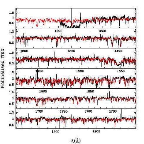
Figure 9: Best fit (red dashed line) of the UV spectrum (black solid line) of HD 46202. The wind parameters are: $\dot{M}$ = $10^{-8.9}$ M_⊙ yr^-1 and $v_{\infty}$ = 1200 km s^-1. X-rays are included so that $\log L_{\rm X}/L_{\rm bol}=-6.05$. The IUE spectrum below 1200 Å is not shown since the low S/N ratio does not allow any reliable comparison.

HD 46202 is an O9 V star situated in the Rosette nebula. An effective temperature of 33000 K gives the best fit of the optical He lines as shown in Fig. 8. As for HD34078, the too deep C ii $\lambda\lambda$6578,6582 doublet may indicate a slightly too low $T_{\mathrm{eff}}$: once again, increasing $T_{\mathrm{eff}}$ by 1000 K improves the fit but gives a worse fit of the He lines, so that we think the value of 33000 K is reasonable within its uncertainty of $\pm$ 2000 K. A gravity of $\log g=4.0$ gives a good fit of the H$\gamma$ line (see Fig. 8).

Figures 8 and 9 show the fit of the wind sensitive lines from which we derive a mass loss rate of 10^-8.9 M_⊙ yr^-1 and a terminal velocity of 1200 km s^-1. According to the X-ray detection, we have chosen $\log\frac{L_{\rm X}}{L_{\rm bol}}=-6.10$ (see Table 4). If X-rays are not included, a value of $\dot{M}$ as low as 10^-10 M_⊙ yr^-1 is required to fit the wind part of C iv $\lambda\lambda$1548,1551. Note that the core of the H$\alpha$ line is stronger in the model, but as the observed profile seems to be somewhat contaminated (possibly by a small nebular contribution), we did not try to fit this core. As C iv $\lambda\lambda$1548,1551 is the main $\dot{M}$ indicator and as $\log\frac{L_{\rm X}}{L_{\rm bol}}$ is quite high for this star, we have run test models including the high ionisation states C V and C VI to check if the C ionisation was modified. They show that the C ionisation is indeed slightly increased, which implies to increase $\dot{M}$ by a factor of $\sim$ 2 in order to fit C iv $\lambda\lambda$1548,1551. Hence, given the uncertainty in $\log\frac{L_{\rm X}}{L_{\rm bol}}$ (due to both uncertainties in $L_{\rm X}$ and $L_{\rm bol}$), we think this effect is negligible compared to other sources of errors for the $\dot{M}$ determination (see Sect. 6). We have also run test models for which the X-ray temperature was increased from 3 $10^{6}$ K to 7 $10^{6}$ K. Fitting C iv $\lambda\lambda$1548,1551 with this new X-ray temperature required a slight increase ($\sim 0.3$ dex) of the mass loss rate. All previous studies give higher values of $\dot{M}$ (see Table 3). As for $v_{\infty}$, the range of values derived by other authors is quite large and encompasses our estimate. This shows the difficulty of deriving $v_{\infty}$ from weak wind line profiles. The low terminal velocity will be discussed in Sect. 7.2.1.

4.4 HD93028

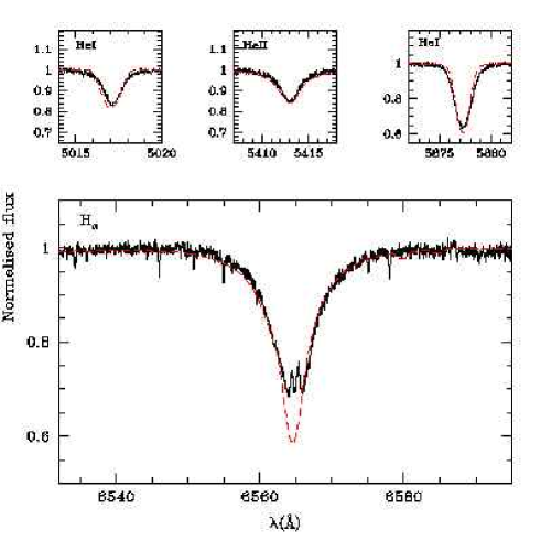
Figure 10: Best fit (red dashed line) of the observed He and H$\alpha$ lines (black solid line) of HD 93028. The effective temperature is 34000 K, $\log g$ = 4.0 and $V$ sin$i$ = 50 km s^-1.

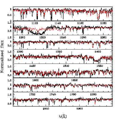
Figure 11: Best fit (red dashed line) of the UV spectrum (black solid line) of HD 93028. For this model, $\dot{M}$ = $10^{-9.0}$ M_⊙ yr^-1, $v_{\infty}$ = 1300 km s^-1and we adopted $\log\frac{L_{X}}{L_{bol}}=-7.0$.

HD 93028 has a spectral type O9V and belongs to the young cluster Collinder 228 in the Carina nebula. A value of $V$ sin$i$ of 50 km s^-1 was deduced from optical lines fits (Fig. 10) and from previous studies (Table 2). The effective temperature we derive from He optical lines is 34000 K.

From the C iv $\lambda\lambda$1548,1551 line, we derive a terminal velocity of 1300 km s^-1, slightly lower than other estimates (see Table 3). We find that a mass loss rate of 10^-9.5 M_⊙ yr^-1 gives a good fit of the far UV, UV and H$\alpha$ spectrum without X rays. However, as we have shown previously, X-rays influences strongly the determination of $\dot{M}$ in stars with weak winds (see Sect. 4.1, 4.3). Hence, although there is no measurement of X-rays for HD 93028, we adopted the classical value $\log\frac{L_{X}}{L_{bol}}=-7.0$ (Chlebowski & Garmany chleb (1991)) and then derived $\dot{M}$ = 10^-9.0 M_⊙ yr^-1 as shown in Figs. 10 and 11. The core of H$\alpha$ is a little too strong in our best fit model, but the observed line shows evidences of interstellar contamination, which is natural in a star forming region (see also the H$\alpha$ profile of HD 93146). The only previous determination of mass loss rate for HD 93028 was made by Howarth & Prinja (hp89 (1989)) who found $\dot{M}$ $=10^{-7}$ M_⊙ yr^-1, more than two orders of magnitude higher than our value.

4.5 HD152590

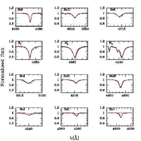
Figure 12: Best fit of the optical spectrum (black solid line) of HD 152590. The effective temperature is 36000 K, $\log g$ = 4.1 and $V$ sin$i$ = 66 km s^-1. The blue dotted line is for a standard model (v_turb = 20 km s^-1 in the computation of the atmospheric structure and v_turb from 5 to 175 km s^-1 for the spectrum) while the red dashed line is for a model with v_turb = 10 km s^-1 (atmospheric structure) v_turb = 10-175 km s^-1 for the spectrum and additional metals (Ne, Ar, Ca and Ni). We see that this improved model leads to better fits of the He I singlet lines, leaving all other lines basically unchanged.

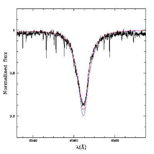
Figure 13: Fits of the observed H$\alpha$ line (black solid line) of HD 152590 for a model with $\dot{M}$ = $10^{-7.78}$ M_⊙ yr^-1 (red dashed line) and for a model with $\dot{M}$ = $10^{-8.75}$ M_⊙ yr^-1 (blue dotted line). The terminal velocity in both models is 1750 km s^-1. Note the insensitivity of H$\alpha$ line profile to the mass loss rate.

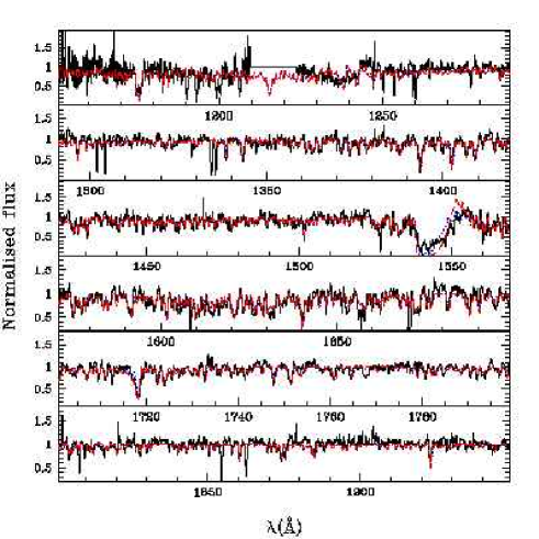
Figure 14: Same as Fig. 13 for the UV range.

HD 152590 is an O7.5Vz star. The distance estimate is difficult since it membership to Trumpler 24, Sco OB1 or NGC 6231 is not completely established. Given the uncertainty in the distance, we simply adopt the mean value (see Table 1).

We adopted $V$ sin$i$ = 66 km s^-1 from Penny (penny (1996)). The optical spectrum shown in Fig. 12 is correctly reproduced with an effective temperature of 36000 K. Note that initially, we had a problem to reproduce the He I singlet lines which were too weak in our models wheras all other lines were very well reproduced. This problem has been recently noted by Puls et al. (puls05 (2005)) when they put forward a discrepancy between CMFGEN and FASTWIND for these lines between 36000 and 41000 K for dwarfs. However, a more complete treatment of line blanketing appeared to solve this problem. Indeed, if we reduce the microturbulent velocity from 20 to 10 km s^-1 in the computation of the atmospheric structure AND if we add some more species (Neon, Argon, Calcium and Nickel) we greatly improve the fit of the He I singlet lines without modifying the strength of other H and He lines (Hillier et al. hil03 (2003) already noted that the He I singlet lines were much more sensitive to details of the modelling than the triplet lines). This is shown in Fig. 12. Note that increasing the microturbulent velocity from 5 to 10 km s^-1 in the computation of the spectrum changes only marginally the line profiles. Hence, we attribute the origin of the discrepancy pinpointed by Puls et al. (puls05 (2005)) to a subtle line-blanketing effect in this particular temperature range, and concerning only the He I singlet lines . Note that reducing v_turb without including additional metals strengthens the singlet lines, but not enough to fit the observed spectrum. Hence the additional line-blanketing effects of Ne, Ar, Ca and Ni, although small (most lines are unchanged) is crucial to fit the He I lines around $T_{\mathrm{eff}}$ = 36000 K. Note that we usually restrict ourselves to models with v_turb = 20 km s^-1 and no Ne, Ca, Ar or Ni since the computational time is much more reasonable. For HD 152590, we found that a gravity $\log g=4.10\pm 0.1$ gives the best fit of the Balmer lines (in particular H$\gamma$)

The terminal velocity of HD 152590 estimated from C iv $\lambda\lambda$1548,1551 is 1750 km s^-1, in good agreement or lower than previous estimates (Table 3). The estimate of the mass loss rate is much more difficult for this star. In fact, we have not been able to fit simultaneously the UV lines and H$\alpha$. If the former are correctly reproduced (with $\dot{M}$ = $10^{-8.75}$ M_⊙ yr^-1), then the later has a too strong absorption in its core, and if H$\alpha$ is fitted (with $\dot{M}$ = $10^{-7.78}$ M_⊙ yr^-1), C iv $\lambda\lambda$1548,1551 is too strong. This is shown in Fig. 13 and 14. We have tried without success to increase the $\beta$ parameter to improve the fit (an increase of $\beta$ leading to a weaker H$\alpha$ absorption). The fits of Fig. 13 and 14 are for $\beta$ = 1.2 and even for this quite high value for a dwarf star, the H$\alpha$ core is not perfectly reproduced. A possible explanation is the presence of a companion for HD 152590 (Gieseking gk82 (1982)). In that case, H$\alpha$ may be diluted by the continuum of this secondary whereas the UV spectrum may be unaffected provided the companion is a later type star than HD 152590 without strong UV lines. However, adopting a conservative approach, we adopt the H$\alpha$ mass loss rate (10^-7.78 M_⊙ yr^-1) as typical, keeping in mind that it may well be only an upper limit.

4.6 HD93146

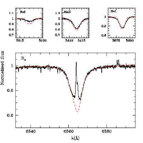
Figure 15: Best fit (red dashed line) of the observed He and H$\alpha$ lines (black solid line) of HD 93146. The effective temperature is 37000 K, $\log g$ = 4.0 and $V$ sin$i$ = 80 km s^-1.

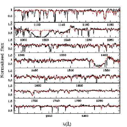
Figure 16: Best fit (red dashed line) of the UV spectrum (black solid line) of HD 93146. For this model, $\dot{M}$ = $10^{-7.25}$ M_⊙ yr^-1and $v_{\infty}$ = 2800 km s^-1.

HD 93146 is an O6.5V((f)) star in the Carina nebula and belongs to the cluster Cr 228.

We adopt $V$ sin$i$ = 80 km s^-1 from our fits and previous determinations (see Table 2). Fig. 15 shows our best fit to the He optical spectrum between 5000 and 6000 Å for which an effective temperature of 37000 K is derived. Notice that this fit is not perfect, but it is actually the best we could get. Increasing $T_{\mathrm{eff}}$ may help reduce the He I absorption, but it increases too much the He II strength. Moreover the UV photospheric lines are very well reproduced with this $T_{\mathrm{eff}}$ (see Fig. 16). As we do not have reliable gravity estimators, we assume $\log g=4.0$ since this value is typical of dwarfs (Vacca et al. vacca (1996), Martins et al. calib05 (2005)).

Fig. 16 shows our best fit of the (far) UV spectrum of HD 93146. The terminal velocity is 2800 km s^-1 and the mass loss rate is 10^-7.25 M_⊙ yr^-1. For higher values, N iv $\lambda$1718 displays a too strong blueshifted absorption. The H$\alpha$ profile of Fig. 15 confirms partly this value of $\dot{M}$ since the line is correctly reproduced, under the uncertainty of the exact depth of the core which is contaminated by nebular emission. Previous estimates are in failry good agreement with the present one (Table 3).

4.7 HD42088

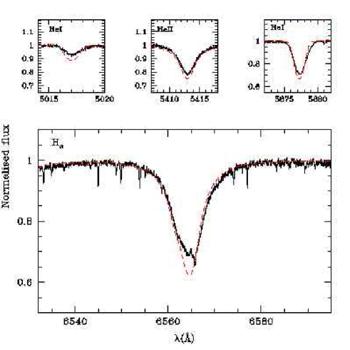
Figure 17: Best fit (red dashed line) of the observed He and H$\alpha$ lines (black solid line) of HD 42088. The effective temperature is 38000 K, $\log g$ = 4.0 and $V$ sin$i$ = 60 km s^-1.

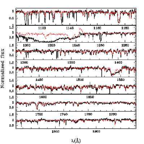
Figure 18: Best fit (red dashed line) of the UV spectrum (black solid line) of HD 42088. For this model, $\dot{M}$ = $10^{-8}$ M_⊙ yr^-1and $v_{\infty}$ = 1900 km s^-1.

HD 42088 is a O6.5 V star associated with the H II region NGC 2175. It also belongs to the class of Vz stars. Note that the distance to this star is poorly constrained so that its luminosity is the least well known of all stars of our sample. The rotational velocity is chosen to be 60 km s^-1 in view of the determinations of Penny (penny (1996)) - 62 km s^-1 - and Howarth et al. (howarth97 (1997)) - 65 km s^-1. The fit of optical He lines above 5000 Å leads to an estimate of the effective temperature which is found to be $\sim$ 38000 K as shown by Fig. 17. This estimate also relies on the fit of UV lines since the number of optical indicators is small. We adopt $\log g=4.0$ (from Vacca et al. vacca (1996)) since we do not have strong gravity indicators.

The terminal velocity is derived from the blueward extension of the absorption in C iv $\lambda\lambda$1548,1551 and is 1900 km s^-1. Previous determinations go from 2030 km s^-1to 2550 km s^-1Given the fact that we adopted a microturbulent velocity of 190 km s^-1in the outer wind (10 % of $v_{\infty}$), the absorption actually extends up to 2100 km s^-1in the model, in good agreement with other determinations. Concerning the mass loss rate, it turns out that a value of 10^-8 M_⊙ yr^-1gives a reasonable fit of the main UV lines and H$\alpha$, although for the latter the very core is not correctly fitted but may suffer from nebular contamination (see Fig. 17). The best fit model is shown in Fig. 18. Our mass loss rate determination based on both H$\alpha$ and UV lines gives a much lower value than ever found for this star (Table 3). But the UV lines produced by models with mass loss rates much higher than our adopted value are much too strong compared to the observed spectrum, forcing us to adopt such a low $\dot{M}$.

4.8 HD93204

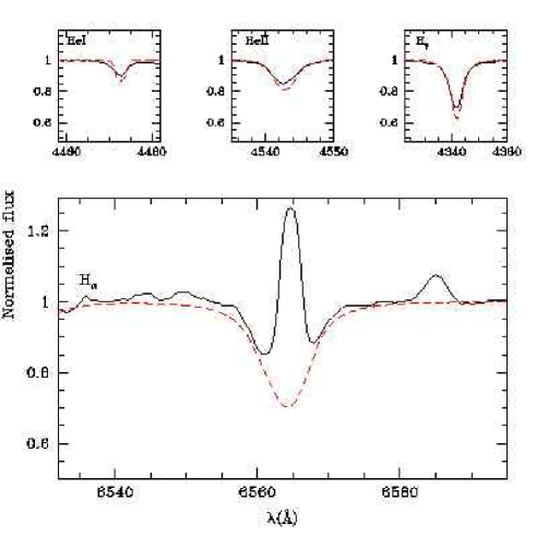
Figure 19: Best fit (red dashed line) of the observed He and H$\alpha$ lines (black solid line) of HD 93204. The effective temperature is 40000 K, $\log g$ = 4.0, $V$ sin$i$ = 130 km s^-1 and $\dot{M}$ = $10^{-6.75}$ M_⊙ yr^-1.

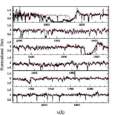
Figure 20: Best fit of the UV spectrum (black solid line) of HD 93204. For this model, $\dot{M}$ = $10^{-6.75}$ M_⊙ yr^-1and $v_{\infty}$ = 2900 km s^-1. The red dashed line is a clumped model with $f_{\infty}=0.1$ and the blue dotted line is a homogeneous model.

HD 93204 (O5V((f))) is a member of the young cluster Trumpler 16 in the Carina complex. We adopt the value 130 km s^-1 for $V$ sin$i$ in our fits, which helps to derive an effective temperature of 40000 K (see Fig. 19) A gravity of $\log g=4.0$ is compatible with the observed Balmer lines.

Fig. 20 shows the fit of the UV spectrum. To fit reasonably all the UV lines, we had to use clumped models. This is especially true for O v $\lambda$1371 since as previously shown by Bouret et al. (jc03 (2003). jc05 (2005)) this line is predicted too strong in homogeneous models. In our case, the use of clumping with the law given in Sect. 3.2 and $f_{\infty}=0.1$ improves the fit of O v $\lambda$1371 as well as N iv $\lambda$1718, as shown in Fig. 20. Reducing $T_{\mathrm{eff}}$ does not solve the problem since in that case O v $\lambda$1371 is weaker but N iv $\lambda$1718 gets stronger. We derive a mass loss rate of 10^-6.75 M_⊙ yr^-1 and a terminal velocity of 2900 km s^-1. Due to the high level of nebular contamination of H$\alpha$, we can not use this line to constrain $\dot{M}$ (see Fig. 19). Our value of $\dot{M}$ is slightly smaller (factor 4) than that of Howarth & Prinja (hp89 (1989)) (Table 3) mainly due to the inclusion of clumping in our models. As for $v_{\infty}$, our estimate is well within the range of values previously derived (see Table 3).

4.9 HD15629

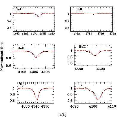
Figure 21: Best fit (red dashed line) of the observed He and H lines (black solid line) of HD 15629. The effective temperature is 41000 K, $\log g$ = 3.75 and $V$ sin$i$ = 90 km s^-1.

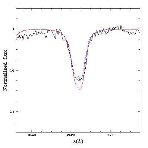
Figure 22: Best fit (red dashed line) of the observed H$\alpha$ line (black solid line) of HD 15629. For this model, $\dot{M}$ = $10^{-6.5}$ M_⊙ yr^-1, $v_{\infty}$ = 2800 km s^-1 and $f_{\infty}=0.1$. We also show a model with $\dot{M}$ = $10^{-5.89}$ M_⊙ yr^-1 and no clumping (blue dotted line) as derived by Repolust et al. (repolust (2004)).

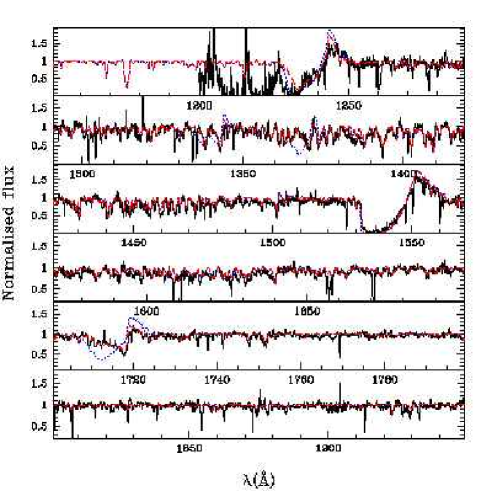
Figure 23: Best fit (red dashed line) of the UV spectrum (black solid line) of HD 15629. The wind parameters are the same as in Fig. 22. The IUE spectrum below 1200 Å is not shown since the low S/N ratio does not allow any reliable comparison. The blue dotted line is the model with the Repolust et al. (repolust (2004)) parameters: note the too strong O v $\lambda$1371 and N iv $\lambda$1718 lines.

HD 15629 is classified as O5V((f)) and belongs to the star cluster IC 1805. The projected rotational velocity is found to be 90 km s^-1 by several authors and we adopted this value which give a good fit of optical and UV photospheric lines. The optical spectrum presented in Fig. 21 indicates an effective temperature of 41000 K. This is in good agreement with the recent determination of Repolust et al. (repolust (2004)) who found 40500 K. We adopted $\log g=3.75$ since it gives a reasonable fit of Balmer lines (Fig. 21) and it is close to the value derived by Repolust et al. (repolust (2004)) who derived $\log g=3.70$.

The best fit model of the UV spectrum is shown in Fig. 23, and H$\alpha$ is displayed in Fig. 22. The main parameters for this model are $\dot{M}$ = $10^{-6.5}$ M_⊙ yr^-1, $v_{\infty}$ = 2800 km s^-1 and $f_{\infty}=0.1$. We also show on these figures a model without clumping and with the mass loss rate of Repolust et al. (repolust (2004)) which is higher - 10^-5.89 M_⊙ yr^-1- than our derived value. Once again the inclusion of clumping is necessary to correctly reproduce both O v $\lambda$1371 and N iv $\lambda$1718. With the Repolust et al. (repolust (2004)) $\dot{M}$ and no clumping, CNO abundances have to be reduced by a factor of 3 to give reasonable fits, and even in that case the O v $\lambda$1371 line is too strong. Such a reduction of the abundances is unlikely for a Galactic star. For our best fit, we have adopted the CNO solar abundances recently claimed by Asplund (asplund04 (2004)) since they are slightly lower than those of Grevesse & Sauval (gs98 (1998)) and allow a fit of the UV lines with a slightly higher (0.25 dex) mass loss rate compared to the later values. Note that in our final best fit, the core of H$\alpha$ is not perfectly fitted. However, we suspect that the strange squared shape of the observed line core is probably contaminated by weak nebular emission. In support of the nebular contamination we note the following: if we adopt the mass loss rate of Repolust et al. (repolust (2004)), the flux level in the line core is correct, but the line is slightly narrower in the remainder of the profile compared to the observed profile, while with our $\dot{M}$, the line is well fitted except in the very core. Increasing the flux level in the core in models with our $\dot{M}$ requires the adoption of $\beta$ = 1.7 which is high for a dwarf. In that case again, although the flux level in the core is correct, the synthetic line profile is too narrow. We are then rather confident that the observed line core is somewhat contaminated and that our mass loss rate is correct. The use of clumping explains partly the discrepancy with the result of Repolust et al. (repolust (2004)). Concerning the terminal velocities, previous extimates range from 2810 to 3220 km s^-1 in reasonable agreement with our value.

4.10 HD46223

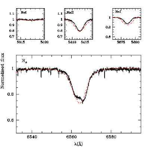
Figure 24: Best fit (red dashed line) of the observed He and H$\alpha$ lines (black solid line) of HD 46223. The effective temperature is 41500 K, $\log g$ = 4.0 and $V$ sin$i$ = 130 km s^-1.

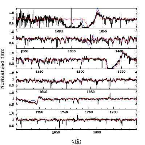
Figure 25: Best fit of the UV spectrum (black solid line) of HD 46223. For this model, $\dot{M}$ = $10^{-6.5}$ M_⊙ yr^-1and $v_{\infty}$ = 2800 km s^-1. The red dashed line is a clumped model with $f_{\infty}=0.1$ and the blue dotted line is a homogeneous model.

HD 46223 belongs to the Rosette cluster (NGC 2244) and has a spectral type O4V((f+)). A projected rotational velocity of 130 km s^-1 was adopted from the fit of optical lines. The upper panels of Fig. 24 show the fit of He optical lines with a model for which $T_{\mathrm{eff}}$ = 41500 K. Note that this effective temperature also gives a reasonable fit of the UV spectrum (see Fig. 25). The subsequently derived stellar parameters are gathered in Table 2. As we do not have reliable gravity indicators, we adopt $\log g=4.0$

As regards the terminal velocity, we find $v_{\infty}$ = 2800 km s^-1 from the UV resonance lines. This is in fairly good agreement with previous estimates (see Table 3). The mass loss rate is derived from H$\alpha$ and the UV resonance lines. The adopted value for $\dot{M}$ is 10^-6.5 M_⊙ yr^-1. As for HD 93204, clumping was necessary to fit O v $\lambda$1371 and N iv $\lambda$1718. Since the inclusion of clumping leads to mass loss rates lower than in homogeneous winds, this explains partly why our estimate is nearly a factor 5 lower than most previous estimates for this star which did not use clumping (see Table 3). Note that in our models, the inclusion of clumping reduces the strength of N v $\lambda$1240 which is then less well fitted than in the case of the homogeneous model. However, the very blue part of the absorption profile is contaminated by interstellar Lyman absorption rendering the exact line profile uncertain.

4.11 HD93250

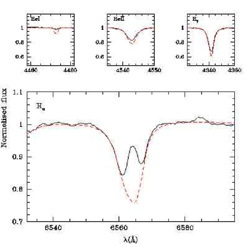
Figure 26: Best fit (red dashed line) of the observed He and H$\alpha$ lines (black solid line) of HD 93250. The effective temperature is 46000 K, $\log g$ = 4.0, $V$ sin$i$ = 110 km s^-1$\dot{M}$ = $10^{-6.25}$ M_⊙ yr^-1, $v_{\infty}$ = 3000 km s^-1 and $f_{\infty}=0.01$.

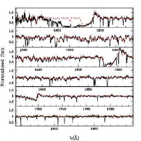
Figure 27: Best fit of the UV spectrum (black solid line) of HD 93250. For this model (red dashed line) $\dot{M}$ = $10^{-6.25}$ M_⊙ yr^-1, $v_{\infty}$ = 3000 km s^-1and $f_{\infty}=0.01$.

HD 93250 is a well studied O dwarf of the Trumpler 16 cluster in the Carina region. It is a prototype of the recently introduced O3.5 subclass (ST O3.5((f+)) Walborn et al. walborn02 (2002)).

Optical lines indicate a projected rotational velocity of 100 km s^-1 and an effective temperature of $\sim$ 46000 K (mainly from the strength of He i $\lambda$4471, see Fig. 26). However, Fe line forests in the UV are more consistent with a value of 42000-44000 K as displayed in Fig. 28. For such a $T_{\mathrm{eff}}$  He i $\lambda$4471 is a little too strong in the model. However, this seems to be the case of all H and He optical lines, possibly due to the fact that HD 93250 may be a binary (see Repolust et al. repolust (2004)) which may also be advocated from the fact that the absorption of C iv $\lambda\lambda$1548,1551 is not black despite the strength of the line (allowing the study of discrete absorption components). Hence, we rely mainly on the UV and we adopt a value of 44000 K for the effective temperature of HD 93250. This value is in reasonable agreement with the determination of Repolust et al. (repolust (2004)) who found 46000 K. We adopted $\log g=4.0$ from Repolust et al. (repolust (2004)) and our fit of H$\gamma$. Note that the estimated mass for this star is especially high (144 M_⊙), which may make HD 93250 one of the highest mass stars known. However, the uncertainty on the mass determination is huge, and HD 93250 is also suspected to be a binary. Hence, we caution that the mass given in Table 2 is only indicative.

The determination of the wind parameters relies on H$\alpha$ and on several strong UV lines: N v $\lambda$1240, O iv $\lambda\lambda$1339,1343, O v $\lambda$1371, C iv $\lambda\lambda$1548,1551, He ii $\lambda$ 1640 and N iv $\lambda$1718. The terminal velocity deduced mainly from C iv $\lambda\lambda$1548,1551 is 3000 km s^-1, slightly lower than the previously derived values which are between 3250 km s^-1 (Repolust et al. repolust (2004)) and 3470 km s^-1 (Bernabeu bernabeu (1989)). However, we use a microturbulent velocity of 200 km s^-1 in the outer part of our model atmosphere for this star, so that in practice, the absorption extends up to 3200 km s^-1. As regards the mass loss rate, we actually found that it was impossible to find a value for $\dot{M}$ which would produce reasonable fits of all UV lines in homogeneous winds. Indeed, O v $\lambda$1371 was always too strong and N iv $\lambda$1718 too weak. Reducing the effective temperature does not improve the situation, since values as low as 40000 K are required to fit O v $\lambda$1371, and in that case the other UV lines are not correctly fitted so that again, we had to include clumping. In the end, we find that a mass loss rate of 10^-6.25 M_⊙ yr^-1with a clumping factor $f_{\infty}=0.01$ gives a reasonable fit, as displayed in Fig. 27. This value of $\dot{M}$ is lower than the determination of Repolust et al. (repolust (2004)) – 10^-5.46 M_⊙ yr^-1– relying only on H$\alpha$. We will return to this in Sect. 7.2.2. Note that the value of $f_{\infty}$ we derive is quite small, but not completely unrealistic in view of recent results presented by Bouret et al. (jc05 (2005)) indicating $f_{\infty}=0.02$ and $0.04$ for two O4 stars.

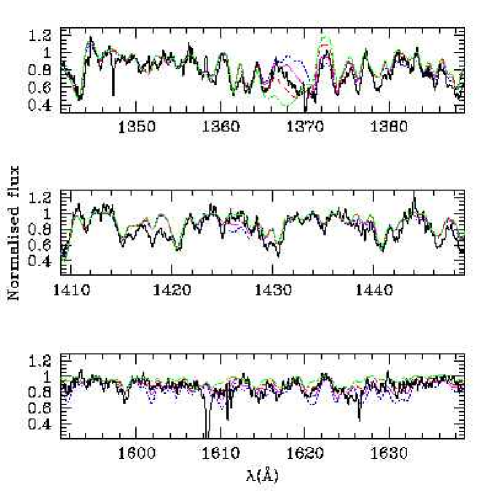
Figure 28: Determination of effective temperature from UV Fe line forests. Solid line is the observed spectrum, dotted line a model with $T_{\mathrm{eff}}$ = 40000 K, long dashed line a model with $T_{\mathrm{eff}}$ = 42000 K, short dashed line a model with $T_{\mathrm{eff}}$ = 44000 K and dot-dashed line a model with $T_{\mathrm{eff}}$ = 46000 K. See text for discussion

5 Role of X-rays and magnetic field in weak-wind stars

Several of our sample stars have published X-ray fluxes. Chlebowski & Garmany (chleb (1991)) report X-ray measurements for HD 38666, HD 46202, HD 152590, HD 42088 and HD 46223, while Evans et al. (evans03 (2003)) give X-ray luminosities for HD 93204 and HD 93250. These high energy fluxes may have important consequences on the atmosphere structure since, as shown by MacFarlane et al. (macfarlane (1994)), the ionisation fractions may be significantly altered. These authors also demonstrated that the effect of X-rays was higher in low-density winds: ionisation in early O stars is almost unchanged by X-rays, while in early B-stars changes as large a factor 10 can be observed between models with and without X-rays. The reason for such a behaviour is that 1) X-rays produce higher ionisation state through single ionisation by high energy photons and the Auger process and 2) the ratio of photospheric to X-ray flux decreases when effective temperature decreases, implying an increasing role of X-rays towards late type O and early B stars (see MacFarlane et al. macfarlane (1994)). Moreover, the lower the density, the lower the recombinations to compensate for ionisations so that we expect qualitatively an even stronger influence of X-rays in stars with low mass loss rate. Since some of our sample stars are late type O stars with low density winds, X-rays can not be discarded in their analysis. Indeed, the Carbon ionisation fraction – and thus the strength of the C iv $\lambda\lambda$1548,1551 line and the derived mass loss rates – can be altered.

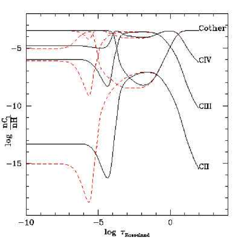
Figure 30: Effect of the inclusion of X-rays on the Carbon ionisation structure. Shown is the ratio of the population of C ionisation state $i$ to the total H population as a function of Rosseland optical depth. The red dashed line corresponds to the model giving the best fit to the UV spectrum when X-rays are not included, while the black solid line is the best fitting model with X-rays. In the former case, C iv is the dominant ionisation state in the wind, while it is no longer the case in the latter model (C V being the dominant). Note that C_other refers to the difference between the total C population and the sum of C ii, C iii and C iv, and is mainly C v here.

In this context, we have first run test models for HD 46202 and HD 93250. For HD 93250, the inclusion of X-rays did not lead to any significant change of the ionisation structure as expected from the above discussion. Indeed, the main wind line profiles were not modified (see also MacFarlane et al. macfarlane (1994), Pauldrach et al. pauldrach94 (1994), pauldrach01 (2001)), indicating that X-rays are not crucial for the modelling of these lines in such high density winds. Of course, other lines are well known to be influenced by X-rays (e.g. O vi $\lambda\lambda$1032,1038) but are not used in this study to derive the stellar and wind parameters. However, in the case of HD 46202 the ionisation structure in the wind is strongly modified which leads to a weaker C iv $\lambda\lambda$1548,1551 line (for a given $\dot{M}$) as displayed in Fig. 29. Indeed, the ionisation fraction of C IV is reduced: this is displayed in Fig. 30 where we see that in the model giving the best fit without X-rays, C iv is the dominant ionisation state, while when X-rays are included, it is no longer the case. Fitting C iv $\lambda\lambda$1548,1551 thus requires a higher mass loss rate. In practice, the change in the C iv $\lambda\lambda$1548,1551 profile when X-rays are included is equivalent to a reduction of the mass loss rate by a factor of $\sim$ 10 in models without X-rays. Given this result, we have included X-rays in our modelling of the atmosphere of HD 38666, HD 46202, HD 34078 and HD93028. For the two former stars, X fluxes from the literature have been used while for the two latter ones, we simply adopted $\log\frac{L_{\rm X}}{L_{\rm bol}}=-7.0$.

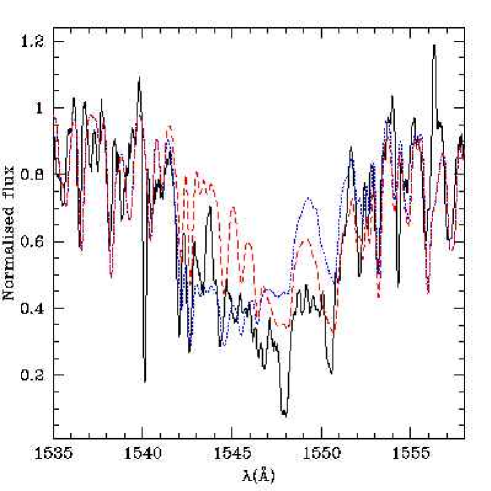
Figure 29: Effect on X-rays on the C iv $\lambda\lambda$1548,1551 line. The observed profile is the solid line, the initial model is the dotted line and the model with X-rays and the same $\dot{M}$ is the dashed line. See text for discussion.

A question which remains to be answered concerning the X properties of such weak wind stars is the origin of the X-ray emission. Indeed, it is usually believed that shocks in the wind due to instabilities in the line driving mechanism are responsible for the production of such high energy photons (Lucy & White lw80 (1980), Owocki, Castor & Rybicki ocr88 (1988)). This scenario seems to apply to the strong wind star Zeta Pup (Kramer et al. kramer03 (2003)). However, recent observations by Chandra have revealed that for the B0V star $\tau$ Sco and for the Trapezium stars, most of the lines emitted in the X-ray range were too narrow to have been produced in the wind up to velocities of the order $v_{\infty}$ as expected in the wind-shock scenario (see Cohen et al. cohen03 (2003), Schulz et al. schulz03 (2003)). And these lines are also not formed very close to the photosphere as predicted by a model in which the X-ray emission is due to a hot corona (e.g. Cassinelli & Olson co79 (1979)). Actually, such lines are more likely to be formed in an intermediate region. This may be explained in the context of magnetically confined winds: in this scenario, the presence of a magnetic field confines the outflow and channels it into the equatorial plane where shocks produce X-ray emission above the photosphere but not in the upper atmosphere (See Babel & Montmerle bm97 (1997)). This model has been recently refined by Ud’Doula & Owocki (uddoula (2002)) who have investigated the structure of both the wind outflow and the magnetic field through time dependent hydrodynamic simulations. In particular, they estimated from simple arguments the strength of the magnetic field required to confine the wind (hereafter $B^{\prime}$) and thus to lead to shocks in the equatorial plane.

In Table 4, we have gathered different properties of the stars of our sample showing X-ray emission: the X-ray luminosity ($L_{\rm X}$), the mechanical wind luminosity ($L_{\rm wind}=\frac{1}{2}\dot{M}v_{\infty}^{2}$) for our $\dot{M}$ and $\dot{M}$ from Vink et al. (vink01 (2001)), and $B^{\prime}$ again considering our derived $\dot{M}$ and Vink’s $\dot{M}$. We see that for weak winds, $\frac{L_{\rm X}}{L_{\rm wind}}$ becomes of the order unity which shows the increasing importance of X-rays as the wind becomes less and less dense. In addition, Table 4 shows that the magnetic field strength required to confine the wind is low for weak-wind stars, showing the increasing role of magnetic field when $\dot{M}$ decreases. Given these results and the above discussion, we may speculate that our weak wind stars may have magnetically confined winds (although no detections of magnetic field exist for them). In that case, one may wonder how our results would be modified. Fig. 8 of Ud’Doula & Owocki (uddoula (2002)) shows that the mass flux ($\rho v$) is reduced close to the pole and enhanced near the equator, but their Table 1 reveals that the total mass loss is only reduced by a factor $<$ 2 even in the case of strong confinement. Hence, using classical 1D atmosphere models should lead to correct values for the mass loss rates within a factor of two, even if magnetic confinement exists.

As regards this last point, a comment on the shape of the line profiles is necessary. Indeed, the only O stars with a detected magnetic field - Theta1 Ori C (Donati et al. donati (2002)) - shows unusual features which may be related to the geometry of magnetically confined wind (Walborn et al. walbornIUE (1985), Gagné et al., gagne (2005)). The absence of such unusual features in the spectra of our stars with weak winds may argue against such a confinement. However, as Theta1 Ori C is the only example and as there is no theoretical prediction of the change in the shapes of wind lines in the presence of magnetic confinement - which also probably depends on the tilt angle between the nagnetic and rotation axis -, we can not completely rule out the existence of magnetic confinement in our weak wind stars.

Table 4: X-ray properties of our sample stars with known X-rays fluxes. $L_{\rm X}$ is from Chlebowski & Garmany (chleb (1991)) for HD 38666, HD 46202, HD 152590, HD 42088 and HD 46223, and from Evans et al. (evans03 (2003)) for HD 93204 and HD 93250. $L_{\rm wind}$ is the mechanical wind luminosity. Values with “Vink” are those for which $\dot{M}$ is taken from Vink et al. (vink01 (2001)) mass loss recipe. $B^{\prime}$ is the value of the magnetic field for which confinement begins (corresponding to $\eta_{\star}=1$ in the formalism of Ud’Doula & Owocki uddoula (2002)).

HD		$\log L_{\rm X}$	$\log\frac{L_{\rm X}}{L_{\rm bol}}$	$\log L_{\rm wind}$	$\log L_{\rm wind}^{Vink}$	$\log\frac{L_{\rm X}}{L_{\rm wind}}$	$\log\frac{L_{\rm X}}{L_{\rm wind}^{Vink}}$	$B^{\prime}$	$B_{Vink}^{\prime}$
		[erg s-1]		[erg s-1]	[erg s-1]			[G]	[G]
38666		31.37	-6.87	32.16	34.25	-0.79	-2.88	7	75
46202		32.40	-6.05	32.76	34.43	-0.36	-2.03	11	72
152590		32.51	-5.86	34.20	34.83	-1.69	-2.32	60	125
42088		32.38	-6.43	34.06	35.89	-1.68	-3.51	33	269
93204		32.06	-7.03	35.67	36.31	-3.61	-4.25	137	286
46223		32.62	-6.53	35.89	36.42	-3.27	-3.80	180	332
93250		33.22	-6.53	36.20	37.20	-2.98	-3.98	153	485

6 Sources of uncertainty for the $\dot{M}$ determination

In this section, we investigate the various sources of uncertainty of our determinations of mass loss rates both on the observational side and on the modelling side.

6.1 Observational uncertainties

Under the term “observational uncertainty”, we gather all the effects which can influence the shape of the observed line profiles, especially H$\alpha$. The first source of uncertainty is the S/N ratio. However, in most of the stars studied here, this ratio is good ($\sim$ 100) and does not affect the analysis. The second source of uncertainty comes from the normalisation of the spectra. This is a general and well known problem which can affect the strength of lines, especially in the case of weak lines. In our spectra the main difficulties arise in the N v $\lambda$1240 and H$\alpha$ regions. For the former, this is due to the presence of the broad Lyman $\alpha$ absorption around 1216 Å which renders uncertain the exact position of the continuum. We simply check that the strength of the emission part of the profile in the models is on average consistent with the observed line, leaving aside the bluest part of the absorption. The case of H$\alpha$ is more critical. The normalisation can be hampered by the S/N ratio: a low ratio will not allow a good identification of the continuum position. The use of echelle spectra renders also difficult the identification of the continuum since the wavelength range around the line of interest in a given order is limited to $\sim$ 60 Å. We estimate that taken together, these effects induce an uncertainty $\lesssim$ 0.02 on the absolute position of the H$\alpha$ core. Of course, H$\alpha$ is also contaminated by nebular emission. When present, such an emission precludes any fit of the very core of the line. But the high resolution of our spectra allows a fit of $\sim 80-90\%$ of the stellar profile, excluding the very core.

6.2 Photospheric H$\alpha$ profile

Our estimates of $\dot{M}$ rely on the fit of both the UV wind sensitive lines and H$\alpha$. In low density winds, H$\alpha$ is essentially an absorption profile for which only the central core is sensitive to mass loss rate. In order to derive reliable values of $\dot{M}$  it is thus important to know how robust the prediction of the photospheric profile is, since it will dominate over the wind emission. This is of much less importance in high density winds where the lines are dominated by wind emission.

To check the CMFGEN prediction in a low density wind, we have compared the H$\alpha$ line with that predicted by FASTWIND, the other non-LTE atmosphere code including wind and line-blanketing widely used for optical spectroscopic analysis of massive stars (see Santolaya-Rey et al. sr97 (1997), Puls et al. puls05 (2005)). The test model was chosen with the following parameters: $T_{\mathrm{eff}}$ = 35000 K, $\log g=4.0$, $\dot{M}$ $=10^{-9}$ M_⊙ yr^-1 and $\beta=0.8$. This set of parameters is typical of the stars with weak winds analysed in the present study, and H$\alpha$ should not be too much contaminated by wind emission. The result of the comparison between CMFGEN and FASTWIND is given in Fig. 31. We see that the agreement between both codes is very good. This is not a proof that the predicted profile is the correct one, but it is at least a kind of consistency check.

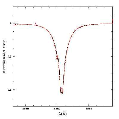
Figure 31: Comparison between CMFGEN (red dashed line) and FASTWIND (black solid line) H$\alpha$ profile. The model is for $T_{\mathrm{eff}}$ = 35000 K, $\log g=4.0$, $\dot{M}$ $=10^{-9}$ M_⊙ yr^-1 and $\beta=0.8$. The agreement between both codes is good.

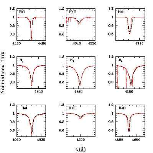
Figure 32: Same as Fig. 31 but for H and He optical lines. The agreement between both codes is good.

We have also investigated another effect which can alter the shape of the H$\alpha$ line core: the number of depth points included in the models. Indeed, the thinner the spatial sampling, the better the line profile. This means that a too coarse spatial grid should introduce errors in the determination of $\dot{M}$ from H$\alpha$. We have run a test model taking the best fit model for HD 34078 and increasing the number of depth points from 72 to 90: a thinner spatial grid leads to a slightly less deep line core, but the difference is only of 0.01 in terms of normalised flux. This is lower than any other observational uncertainty (see Sect. 6.1) so that we have adopted $\sim$ 70 depth points in all our computations .

In conclusion, there is no evidence that the photospheric H$\alpha$ profile is not correctly predicted by our models.

6.3 Ionisation fraction

In the low density winds, which correspond to late O type dwarfs in the present study, the final word concerning the mass loss rate is often given by C iv $\lambda\lambda$1548,1551. Indeed, H$\alpha$ becomes almost insensitive to $\dot{M}$ in these cases, and the other main wind sensitive UV line, N v $\lambda$1240, is almost absent from the spectra due to the reduced effective temperature. Other indicators such as Si iv $\lambda\lambda$1394,1403 or N iv $\lambda$1718 are still present, but they are weaker than C iv $\lambda\lambda$1548,1551 and become rapidly insensitive to any change of the mass loss rate. For more standard winds, almost all indicators can be used together to derive $\dot{M}$. We show in Fig. 33 the variation of the C iv $\lambda\lambda$1548,1551 line profile when the mass loss rate is decreased from 10^-8.5 down to 10^-9.5 M_⊙ yr^-1 for the case of star HD 46202. We clearly see that C iv $\lambda\lambda$1548,1551 is still sensitive to changes in $\dot{M}$ even for such low values. In parallel, we see that H$\alpha$ is essentially unchanged in this regime of $\dot{M}$.

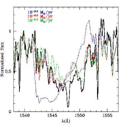
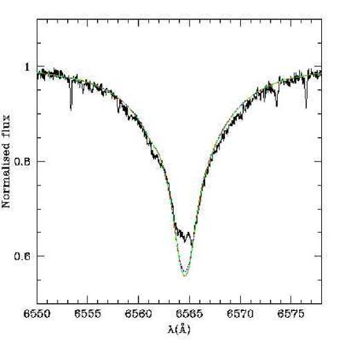
                               (a)                                                                       (b)

Figure 33: Determination of $\dot{M}$ in low density winds (HD 46202). (a) shows the variation of the C iv $\lambda\lambda$1548,1551 line profile when $\dot{M}$ is reduced (solid line: observed line; dash-dotted line: $\dot{M}$ = $10^{-8.5}$ M_⊙ yr^-1; long dashed line: $\dot{M}$ = $10^{-8.9}$ M_⊙ yr^-1; short-dashed long-dashed line: $\dot{M}$ = $10^{-9.5}$ M_⊙ yr^-1). Notice that the weaker the line, the more prominent the presence of photospheric lines (mostly from iron) superimposed to the C iv absorption. (b) shows the behaviour of H$\alpha$ under the same changes. See text for discussion.

However, relying on only one line to assign final mass loss rates may be risky. We have highlighted in paper I that erroneous mass loss rates may be derived in the case where the C IV ionisation fraction is incorrectly predicted. This is still true here, since fitting the observed profile gives the right value of $\dot{M}\times q_{C\leavevmode\nobreak\ {\sc IV}}$ ($q_{C\leavevmode\nobreak\ {\sc IV}}$ being the ionisation fraction of C IV) but not necessarily the right $\dot{M}$. In Fig. 34, we compare the ionisation fractions predicted by the CMFGEN best fit models to the values derived by Lamers et al. lamers99 (1999) (hereafter L99) for dwarfs. The ionisations fractions are defined by

$$q_{C\leavevmode\nobreak\ {\sc IV}}=\frac{\int^{1}_{0.2}n_{C\leavevmode\nobreak\ {\sc IV}}(x)dx}{\int^{1}_{0.2}n_{C}(x)dx}$$ (7)

where $x=\frac{v}{v_{\infty}}$ and $n_{C\leavevmode\nobreak\ {\sc IV}}$ and $n_{C}$ are the number densities of C IV and C respectively. At first glance, the CMFGEN ionisation fractions seem to be $\sim$ 2 orders of magnitude higher than the L99 results, and that in spite of the few lower limits in the latter data. However, several comments can be made:

- First, the work of L99 is based on previous mass loss rate determinations, mainly from H$\alpha$ (Puls et al. puls96 (1996), Lamers & Leitherer ll93 (1993)) or from predictions for their dwarf subsample (Lamers & Cassinelli lc96 (1996)). In the latter case, $\dot{M}$ is derived from the modified wind momentum - luminosity relation, so that any error in the calibration can lead to incorrect mass loss rate. Moreover, the uncertainty of such a method due to the fact that a given star can deviate from a mean relation may introduce a bias in the derived ionisation fraction. Concerning the mass loss rates derived from H$\alpha$, Lamers & Leitherer (ll93 (1993)) use the line emission strength to determine $\dot{M}$. However, in most O dwarfs H$\alpha$ is in absorption so that the determination of the emission part of the line filling the photospheric profile may be uncertain. Puls et al. (puls96 (1996)) also use H$\alpha$ to derive $\dot{M}$ but give only upper limits in the cases of thin winds. As L99 adopt these upper limits as the real values, we should expect the derived ionisation fractions to be lower limits.

- Second, there is a significant shift in terms of parameter space sampled by our results and that of L99: we have stars with $33000<T_{\rm eff}<44000$ K and $-17.3<\log<\rho><-14.4$ (where $<\rho>=\frac{\dot{M}}{4\pi r^{2}_{0.5}}\frac{2}{v_{\infty}}$ and $r_{0.5}$ is the radius at which the velocity reaches half the terminal velocity) while L99 have $38000<T_{\rm eff}<50500$ K and $-15<-log<\rho><-13.4$, although both studies have stars of late and early O spectral types. Concerning effective temperatures, part of the discrepancy comes from the use of line-blanketing in our models, which is known to reduce $T_{\mathrm{eff}}$ compared to unblanketed studies. But for densities, the explanation may again come from the fact that the adopted mass loss rates (and consequently the densities) in one or the other study are not correct. Can we discriminate between them? An interesting point is that 3 stars are common to our study and that of L99: they are shown linked by dotted lines in Fig. 34. If we consider the fact that line-blanketing may explain the lower $T_{\mathrm{eff}}$ in our study, and the fact that for these stars the ionisation fractions derived by L99 are only lower limits, then the ionisation fractions predicted by CMFGEN are not necessarily too high. And if in addition we argue that our study investigates a density range not explored by L99, then we can not conclude that the ionisation fractions predicted by CMFGEN are wrong since no comparison can be made for very low mean densities.

How could we test more strongly the wind ionisation fractions of our atmosphere models? One possibility is offered by the analysis of far UV spectra. Indeed, this wavelength range contains a number of lines formed in the wind from different ions of the same elements. Such a test will be done in a subsequent paper, based on FUSE observations of Vz stars in the LMC. But we can already mention that several studies of supergiants in the Magellanic Clouds using FUSE + optical data do not reveal any problem with the CMFGEN wind ionisation fractions, except that clumping must be used to reproduce a couple of (but not all) lines (see Crowther et al. paul02 (2002), Hillier et al. hil03 (2003), Evans et al. evans04 (2004)). Hence in the following, we assume that the ionisation fractions given by CMFGEN are correct.

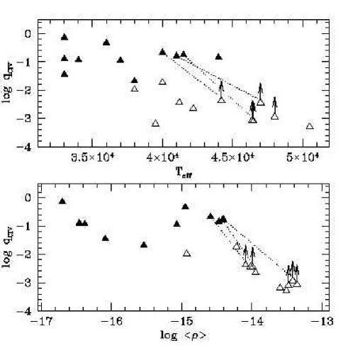
Figure 34: C IV ionisation fractions in CMFGEN models (filled symbols) and from Lamers et al. lamers99 (1999) (open symbols) for dwarfs as a function of effective temperature (upper panel) and mean wind density (lower panel). The dotted lines link objects in common between this work and the study of Lamers et al. (lamers99 (1999)). See text for discussion.

6.4 Abundances

Although our mass loss determination relies on both H$\alpha$ and UV lines, we usually give more weight to the UV diagnostics since the absorption profile of H$\alpha$ can be shaped by other parameters than $\dot{M}$ ($\beta$, clumping). But the UV lines depend more strongly on abundances than H$\alpha$. Hence, we have to estimate the error we make on the $\dot{M}$ determination from UV lines due to uncertain abundances. We have already seen in Sect. 4.9 that adopting the CNO abundances of Asplund (asplund04 (2004)) instead of those of Grevesse & Sauval (gs98 (1998)) – which corresponds on average to a reduction by a factor of $\sim$ 3/4 – leads to an increase of $\dot{M}$ by 0.25 dex. We have also run test models for a low luminosity star (HD 46202). It turns out that reducing the CNO abundances by a factor 2 implies an increase of the mass loss rate of the order of 2-2.5 in order to fit C iv $\lambda\lambda$1548,1551 since this line is not saturated in low density winds and thus its strength is directly proportional to the number of absorbers..

How different from solar could the CNO abundances of our sample stars be ? Given the estimated distances, it turns out that all stars are within 3 kpc from the the sun. Determinations of abundances through spectroscopic analysis of B stars (Smartt et al. smartt_ab (2001), Rolleston et al. rolleston (2000)) reveal the following gradients: $-0.07$ dex/kpc for C, O and Si, and $-0.06$ to $-0.09$ dex/kpc for N. Similarly, Pilyugin et al. (pilyugin (2003)) derive an Oxygen abundance gradient of $-0.05$ dex/kpc from studies of HII regions. Taken together, these results indicate that on average we do not expect variation of CNO abundances by more than $\pm$ 0.25 dex for our sample stars. This means that adopting a solar metallicity leads to an error of at most 0.3 dex on the mass loss rate determination.

Given the above discussion, we estimate the error on $\dot{M}$ due to uncertainties in the CNO abundances to be of $\sim$ 0.3 dex.

6.5 Advection / adiabatic cooling

In low density winds, two processes may affect the ionisation structure: advection and adiabatic cooling. The former is rooted in the fact that for low densities, the timescale for recombinations becomes longer than the timescale for transport by advection. Thus the ionisation structure can be significantly changed. The latter process (adiabatic cooling) lowers the temperature in the outer part of the atmosphere where the heating processes (mainly photoionisations) are less and less efficient due to the low density, implying also a modification of the ionisation structure (see also Martins et al. n81 (2004)). We have tested the influence of those two effects in one of our low $\dot{M}$ models for HD 46202. Their combined effects lead to an increased ionisation in the outer atmosphere, the mean ionisation fraction of C IV being lowered by $\sim$ 0.1 dex (which does not modify the conclusions of Sect. 6.3). This slightly changes the UV line profiles, especially C iv $\lambda\lambda$1548,1551  which for a given $\dot{M}$ shows a smaller absorption in the bluest part of the profile. Quantitatively, the inclusion of advection and adiabatic cooling is equivalent to an increase of $\dot{M}$ by $\sim$ 0.15 dex. We have thus included these two processes in our models for low density winds (HD 38666, HD 34078, HD 46202, HD 93028).

Given the above discussions, we think our $\dot{M}$ determinations have a very conservative error bar of $\pm 0.7$ dex (or a factor $\pm$ 5). This is a quite large uncertainty which however does not modify qualitatively our results, namely the weakness of O dwarfs with low luminosity (see Sect. 7.2.2).

7 Discussion

7.1 Evolutionary status

Fig. 35 shows the HR diagram of the our sample stars. Overplotted on Fig. 35 is our new calibration $T_{\mathrm{eff}}$ - luminosity (Martins et al. calib05 (2005), solid line) for dwarfs: most stars of our sample agree more or less with this relation (within the error bars). The latest type stars of our sample, which are also the stars showing the weakest winds, may be slightly younger than “standard” dwarfs of the same spectral type (or $T_{\mathrm{eff}}$). Notice that this does not mean that these stars are the youngest in terms of absolute age, but that they are less evolved than classical dwarfs. Indeed, the youngest stars of our sample are those of Trumpler 16 (HD 93250 and HD 93204) for which we derive an age of 1 to 2 Myrs, compatible with the $L-$ $T_{\mathrm{eff}}$ relation. In comparison, HD 38666 and HD 34078 may be 2 to 4 Myrs old according to our HR diagram (although given the error bars, we can not exclude younger ages), slightly less than for standard late type dwarfs. In the scenario where these two stars originated from a binary and were ejected in a dynamical interaction, Hoogerwerf et al. (hbz01 (2001)) estimate a travel time of 2.5 Myrs, while van Rensbergen et al. (vr96 (1996)) found travel times of $\sim$ 3.5 Myrs for HD 38666 and $\sim$ 2.5 Myrs for HD 34078. These estimates are in good agreement with our results. We also derive an age of $\sim$ 3-5 Myrs HD 46202, one of our weak wind stars. Note that this star is in the same cluster as HD 46223 which is likely 1-2 Myrs old according to Fig. 35. A similar age should be expected for these two stars in case of a burst of star formation, but an age spread of 1-2 Myrs (common in star clusters) can explain the difference. The same is true for the stars of Cr 228: HD 93146, the brightest star, may be slightly younger than HD 93028.

HD 152590 behaves differently, being less luminous than other dwarfs of same $T_{\mathrm{eff}}$. It is interesting to note that this star is classified as Vz. Taking literally the result of Fig. 35, it seems indeed that it is younger than other dwarfs (but again, the error bars are large), confirming the fact that Vz stars are supposed to lie closer to the ZAMS than typical dwarfs. However, HD 42088 is another Vz star of our sample, and it has a more standard position on the HR diagram. This poses the question of the exact evolutionary status of Vz stars. Indeed, they are defined by stars having He ii $\lambda$4686 stronger than any other He II lines which is thought to be a characteristic of youth since this line is filled with wind emission when the star evolves. In fact the Vz characteristics may be more related to the wind properties than to the youth of the star. Indeed, HD 42088 seems to have the same stellar properties as HD 93146, but the former is classified Vz (not the latter) and has a weaker wind ($\dot{M}$ = $10^{-8}$ M_⊙ yr^-1 compared to $10^{-7.25}$ M_⊙ yr^-1 for HD 93146. Note however that the distance (and thus luminosity) of HD 42088 is highly uncertain. Obviously, more studies are required to better understand the physics of Vz stars.

To summarise, there may be a hint of a link between a relative youth and the weakness of the wind if by youth we mean an evolutionary state earlier than for standard stars and not an absolute age, standard stars meaning stars with the average properties of dwarfs studied so far. But the present results are far from being conclusive. A forthcoming study of Vz stars in the LMC will probably shed more light on this issue.

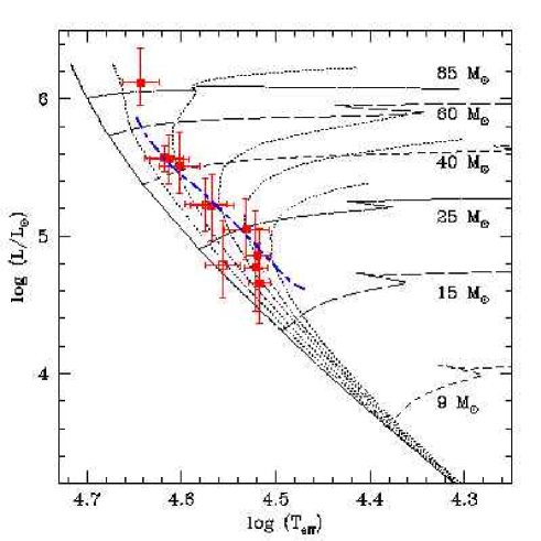
Figure 35: HR diagram of the Galactic stars. Evolutionary tracks are from Lejeune & Schaerer (lejeune (2001)) and Z = Z_⊙. Isochrones for 0, 1.. 5 Myrs are indicated together with evolutionary paths of stars of different masses. The blue dashed line is our new relation $T_{\mathrm{eff}}$ - luminosity for dwarfs (Martins et al. calib05 (2005)). Squares are the stars studied here (open symbols are for Vz stars).

7.2 Wind properties

7.2.1 Terminal velocities

Some of the terminal velocities we derive are surprisingly low (see Table 2) reaching values lower than the escape velocity in a one case (HD 34078). What could explain this behaviour? First, the most obvious reason could be an underestimation of $v_{\infty}$. We have argued in paper I that in stars with weak winds the density in the upper parts of the atmosphere may be so low that almost no absorption takes place in strong lines usually formed up to the top of the atmosphere. This explanation was also given by Howarth & Prinja (hp89 (1989)) to justify the low $v_{\infty}$ they obtained in some stars. If this is indeed the case, one would expect a smooth decrease of the absorption strength in the blue part of P-Cygni profiles due to the reduction of the density as we move outwards, and not a steep break as seen in dense winds. Is there such a transition? Fig. 36 shows the C iv $\lambda\lambda$1548,1551 line profiles of HD 34078 and HD 46223 and reveals that although the increase of the flux level from the deepest absorption to the continuum level in the bluest part of the profile extends over a slightly larger range in the case of the weak wind star (3 Å for HD 38666 instead of 2 Å for HD 46223), it is difficult to draw any final conclusion as regards the reduction of the C iv $\lambda\lambda$1548,1551 absorption in the outer wind of low density wind stars from this simple eye estimation given also that blending is clearly apparent in the line of HD 38666. More information is given by Fig. 37 which shows the derived terminal velocities as a function of mean density in the wind (see Sect. 6.3 for definition). There is an obvious trend of lower terminal velocities with lower wind densities. This is not a proof of the fact that absorption in strong UV lines extends to larger velocities since low densities also mean low mass loss rate and correspond to stars with lower radiative acceleration. However, it is an indication that underestimations of $v_{\infty}$ are certainly more likely to happen in such low density stars.

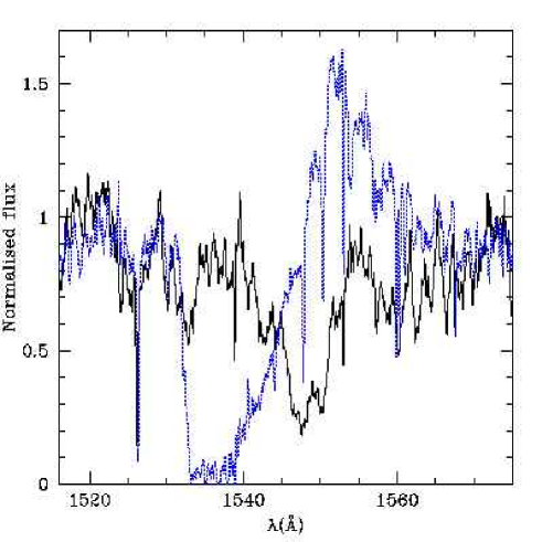
Figure 36: Comparison between C iv $\lambda\lambda$1548,1551 line profiles in a star with weak (HD 38666, solid line) and strong (HD 46223, dotted line) wind. The rise of the flux level in the very blue part of the absorption features is slightly shallower in HD 38666. See text for discussion.

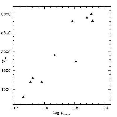
Figure 37: Terminal velocity as a function of mean density in the wind for the stars studied here. There is a clear trend of lower $v_{\infty}$ in lower density winds.

In view of the above discussion, it is not clear whether the lower density in the outer atmosphere of weak wind stars is responsible for an underestimation of the terminal velocities. But we can not exclude that our estimates of $v_{\infty}$ are lower than the true values in low density winds. Now, with this in mind, let us now assume for a moment that the derived values are real terminal velocities: what are the implications? The radiation driven wind theory predicts that $v_{\infty}$ is tightly correlated to the escape velocity (v_esc) according to

$$v_{\infty}^{2}=v_{esc}^{2}I(\alpha)\frac{\alpha}{1-\alpha}$$ (8)

where $\alpha$ is the usual parameter of the Castor, Abbott & Klein (cak (1975)) formalism and $I(\alpha)$ is a correction factor to take into account effects of the finite cone angle of the star disk (see Kudritzki et al. kud89 (1989)). In practice, it is possible to derive values of $\alpha$ from this equation once the stellar parameters and $v_{\infty}$ are known. The only problem comes from $I(\alpha)$ which is a complex function of (among other parameters) $\alpha$. However, it is possible to solve this problem with the following procedure: we first assume a given value of $\alpha$, then estimate $I(\alpha)$ which is subsequently used to find a new $\alpha$ using

$$\alpha=\frac{\frac{v_{\infty}^{2}}{v_{esc}^{2}}}{I+\frac{v_{\infty}^{2}}{v_{esc}^{2}}}$$ (9)

A few iterations should lead to the final value of the $\alpha$ parameter. We have used such a scheme to estimate $\alpha$ for our sample stars and for a number of stars studied elsewhere (Herrero et al. her00 (2000), hpn02 (2002), Repolust et al. repolust (2004) and Markova et al. mark04 (2004)). Solutions are usually found with less than 10 iterations (and are essentially independent on the starting value of $\alpha$), except in the cases where $v_{\infty}$/v_escwas larger than $\sim 3$: in that case, the iterative process did not converge but kept oscillating between two distinct values. The results for the cases where solutions could be found are shown in Fig. 38 (lower panel). A majority of cases lead to $\alpha\sim 0.5-0.6$, in reasonable agreement with (although slightly lower than) theoretical expectations (Puls, Springmann & Lennon psl00 (2000)). However, for the stars of this work with weak winds (and low $v_{\infty}$), lower values are deduced ($\alpha\sim 0.3$). Hence, if the derived low terminal velocities correspond to real $v_{\infty}$, they may be due to low values of the $\alpha$ parameter (given Eq. 8.) If true, this may also have important implications for the scaling relations involving mass loss rates (see next section). Again, it may be possible that we underestimate the terminal velocities, but the above possibility is worth being discussed in view of the puzzle of the weak winds. Note that we have also plotted in Fig. 38 the ratio of terminal to escape velocity which is usually of the order 2.6 for O stars with $T_{\mathrm{eff}}$ $>$ 21000 K (Lamers et al. lamers95 (1995)). We see that hottest stars of our sample follow this general trend whereas stars with weak winds have much lower ratios.

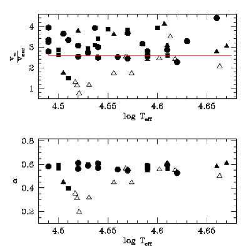
Figure 38: Upper panel: ratio of terminal to escape velocity in our sample stars (open symbols) and stars studied by Herrero et al. her00 (2000), hpn02 (2002), Repolust et al. repolust (2004) and Markova et al. mark04 (2004) (filled symbols). The solid line indicates the classical value 2.6 derived for stars hotter than 21000 K (Lamers et al. lamers95 (1995)). Dwarfs (giants, supergiants) are shown by triangles (squares, circles). Lower panel: derived $\alpha$ parameter from the estimated terminal and escape velocities. See text for discussion.

Another very interesting explanation for the low terminal velocities we derive (again assuming that they are the real values) is the effect of X-rays. Indeed, Drew et al. (drew94 (1994)) highlighted the fact the cooling time in the outer atmosphere of massive stars with relatively weak winds (late O / B stars) can become relatively high so that in the case where X-rays possibly emitted by shocks heat the outer atmosphere, this region remains hot. In that case, the ionisation structure is strongly modified compared to the inner atmosphere and in practice, the radiative force becomes negligible in this hot region. This means that the wind keeps expanding at the velocity reached at the top of the “cool” region which is lower than the value predicted by the radiation driven wind theory. This effect should be checked in future hydrodynamical simulations.

7.2.2 Mass loss rates and modified wind momenta

The mass loss of O stars has been known for a long time to depend on luminosity since due to the basic mechanism of radiatively driven winds, the more photons are available, the larger the acceleration and the larger the mass loss rate (e.g. Castor, Abbott & Klein cak (1975), Kudritzki & Puls kp00 (2000)). Fig. 39 shows mass loss rates for our sample stars (filled symbols) and stars from other studies (Herrero et al. her00 (2000), hpn02 (2002), Repolust et al. repolust (2004) and Markova et al. mark04 (2004), open symbols) as a function of luminosity. One sees that there is a good correlation between $\dot{M}$ and $L$ for bright stars. Note however that our sample stars seem to show lower $\dot{M}$ than what could be expected from the other studies (see also Table 3). For low luminosity stars, the correlation still exists, but the scatter is much larger. Moreover, the slope of the relation seems to be steeper for these objects, the transition luminosity being $\log\frac{L}{L_{\odot}}\sim 5.2$. Although our work is the first to show such a behaviour based on quantitative modelling of atmosphere of O stars, this trend was previously mentioned by Chlebowski & Garmany (chleb (1991)) and Lamers & Cassinelli (lc96 (1996)). This result confirms our finding of paper I in which we showed that the stellar components of the star forming region SMC-N81 displayed winds weaker than expected from the relation $\dot{M}$ - $L$ at high luminosities. In paper I, we mentioned that a possible explanation of such a weakness was the reduced metallicity of the SMC, but we also showed that the Galactic star 10 Lac had the same low mass loss rate. Here, we confirm that several Galactic stars with low luminosity indeed show low $\dot{M}$, rendering unlikely the effect of metallicity alone.

We also showed in paper I that the winds were weaker than predicted by the current hydrodynamical simulations. Fig. 40 extends this trend for the Galactic stars studied here: in the “worst” cases, the difference between our derived $\dot{M}$ and the mass loss rates predicted by Vink et al. (vink01 (2001)) can reach 2 orders of magnitude! Note that even for bright stars our values are lower than the predictions but only by a factor $\lesssim$ 5. This is mainly due to the introduction of clumping in our models for these stars which naturally leads to reduced mass loss rates (Hillier et al. hil03 (2003), Bouret, Lanz & Hillier jc05 (2005)). Using a different approach, Massa et al. (massa03 (2003)) also hilighted the possibility of lower mass loss rates due to the presence of clumping. We will come back to this below.

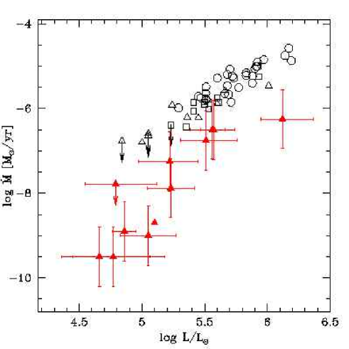
Figure 39: Mass loss rates as a function of Luminosity for Galactic O stars. The filled triangles are the dwarfs studied in the present paper (+ 10 Lac from paper I displayed by the filled triangle without error bars). Open symbols are data from Herrero et al. (her00 (2000), hpn02 (2002)), Repolust et al. (repolust (2004)) and Markova et al. (mark04 (2004)). Triangles (squares, circles) are for dwarfs (giants, supergiants).

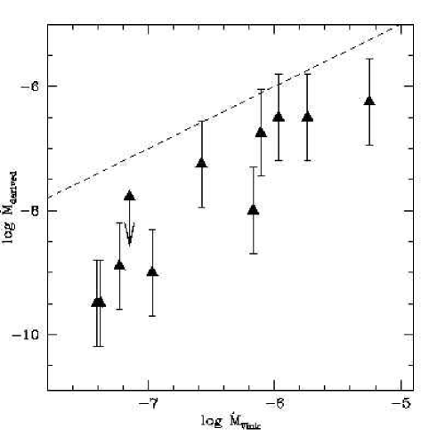
Figure 40: Comparison between derived mass loss rates and predictions of hydrodynamical simulations (Vink et al. vink01 (2001)).

One may also wonder why our values of $\dot{M}$ are lower than other previous studies. Indeed, as shown by Table 3 our mass loss rates are systematically lower than derived so far for all stars of the sample. How can we explain this behaviour? First, let us recall that the mass loss rates gathered in Table 3 are estimated from either pure H$\alpha$ analysis (Leitherer leith88 (1988), Lamers & Leitherer ll93 (1993), Puls et al. puls96 (1996), Repolust et al. repolust (2004), Markova et al. mark04 (2004)) or from pure UV analysis (Howarth & Prinja hp89 (1989), Chlebowski & Garmany chleb (1991)).

The H$\alpha$ study of Leitherer (leith88 (1988)) and Lamers & Leitherer (ll93 (1993)) relied on measurement of H$\alpha$ emission equivalent widths. They are linked with H$\alpha$ luminosities which are themselves related to mass loss rates. The relation L(H$\alpha$) - $\dot{M}$ is based on estimates of the population of the third level of Hydrogen for which departure coefficients from LTE are taken from the pure H He computations of Klein & Castor (kc78 (1978)). The H$\alpha$ emission equivalent width is calculated from the total equivalent width to which a photospheric profile from the plane-parallel pure H He models of Auer & Mihalas (am72 (1972)) is subtracted. This procedure may suffer from various approximations: the use of pure H He models may introduce errors in the prediction of departure coefficients since line-blanketing is known to affect the ionisation (and excitation) structure; moreover, photospheric profiles based on H He plane-parallel models may also be different from line-blanketed spherically extended models. In the case of stars with H$\alpha$ in absorption, the estimate of the emission part may be risky since it may suffer from uncertainties in the photospheric component subtraction, from contamination by interstellar lines or from errors in normalisation process. Leitherer (leith88 (1988)) himself argues that the wind emission part of the global (wind + photospheric) profile becomes almost undetectable in stars with H$\alpha$ in absorption. Hence, the H$\alpha$ mass loss rates of such objects based on this method is rather uncertain.

Another method relying on H$\alpha$ is that of Puls et al. (puls96 (1996)) and Markova et al. (mark04 (2004)). It is again based on the emission part of H$\alpha$ which is related to mass loss rate through an estimate of the H departure coefficient under the Sobolev approximation. Their method is accurate for values of their parameter A $>10^{-4}$ (see Eq. (3) of Puls et al. for a definition of A) which, for typical values of the stellar parameters of O stars, corresponds roughly to $\dot{M}$ $>10^{-7}$ M_⊙ yr^-1. This is mainly the reason why the authors give only upper limits for stars with H$\alpha$ in absorption. Finally, Repolust et al. (repolust (2004)) used FASTWIND (see Sect. 6.2) to fit the H$\alpha$ profile and estimate $\dot{M}$. In the case of weak winds, this method becomes less and less accurate since H$\alpha$ is almost entirely photospheric and hardly depend on mass loss. Here again, the authors only give upper limits on $\dot{M}$ in those cases.

Concerning UV based determinations of the mass loss rate, Howarth & Prinja (hp89 (1989)) use the column densities in several UV lines to estimate $\dot{M}\times qi$ ($qi$ being the ionisation fraction of the ion responsible for the line studied). Under the approximation that the ionisation fraction is independent of luminosity, they derive $\dot{M}$. The latter approximation may introduce errors in the mass loss rates estimate. Indeed, our modelling of massive stars atmospheres reveals that the ionisation fractions are not constant when $T_{\mathrm{eff}}$ changes among dwarf stars (which in this case reduces to a change of luminosity, see Fig. 34). Since the largest ionisation fractions of C IV given by Howarth & Prinja (hp89 (1989)) are of the order 10^-2.5 (see their Fig. 16) while we find values as high as $\sim$ 10^-0.5, a factor of 100 between their $\dot{M}$ and ours is possible.

The other UV analysis to which our results are compared is that of Chlebowski & Garmany (chleb (1991)). The authors use fits of the UV lines using the method of Olson (olson (1982)) which is similar to the SEI method (Lamers et al. lamers87 (1987)). Basically, this method uses a parameterisation of the optical depth through the line profile to produce synthetic profiles which, once compared with observed spectra, allow a determination of $\dot{M}$. However, this latter step requires a few approximations. In particular, the ionisation fraction has to be estimated which involves the use of SED at high energies (i.e. close to ionisation thresholds of C IV and N V): a blackbody distribution is used in the computations of Chlebowski & Garmany (chleb (1991)). Moreover, only photoionisation and recombinations from/to the ground states are taken into account. Hence, once again the ionisation fractions may not be correctly predicted leading to errors on $\dot{M}$. However, it is interesting to note that the approach of Chlebowski & Garmany (chleb (1991)) is more accurate than that of Howarth & Prinja (hp89 (1989)) as regards the ionisation fractions and leads to lower mass loss rates (see Table 3), so that if, as we can expect, the ionisation fractions are better predicted in the current atmosphere models and are in fact higher, lower mass loss rates are not too surprising.

Another important point highlighted in paper I was the behaviour of the so called modified wind momentum - luminosity relation (WLR) at low luminosities. Indeed, we showed that there seemed to be a breakdown of this relation below $\log\frac{L}{L_{\odot}}\simeq 5.2$, at least for stars of the SMC (including the stars of paper I and 3 stars of NGC 346 studied by Bouret et al. jc03 (2003)). The Galactic star 10 Lac also showed a reduced wind momentum, indicating that this property could not be related to metallicity alone. In the present study, several characteristics of the WLR are highlighted.

We first confirm that there is a breakdown - or at least a steepening- of the WLR below $\log\frac{L}{L_{\odot}}\simeq 5.2$. Indeed, Fig. 42 shows that most stars below this transition luminosity have wind momenta lower that what one could expect from a simple extrapolation of the WLR for bright stars. Indeed, for $\log\frac{L}{L_{\odot}}\sim 5.0$, the relation for dwarfs + giants found by Repolust et al. (repolust (2004)) gives wind momenta of the order $10^{28}$ while we find values as low as $10^{25}$! There is in fact only one object which is marginally in agreement with the relation of Repolust et al. (repolust (2004)), but we have only an upper limit for $\dot{M}$ for this star (HD 152590).

Second, we find that for the bright stars of this study, the modified wind momenta are reduced compared to the pure H$\alpha$ analysis on which the WLR is established. The difference is on average a factor of between 5 and 10, especially for the two objects we have in common (HD 15629 and HD 93250). The explanation of this discrepancy comes from the use of clumping in our models for these stars. Indeed, it is necessary to use inhomogeneous winds to correctly fit a number of UV lines, especially O v $\lambda$1371 and N iv $\lambda$1718. In Fig. 41 we show the UV + H$\alpha$ spectra of HD 93250 and two models: one with the mass loss rates derived by Repolust et al. (repolust (2004)) from H$\alpha$ only ($\dot{M}=10^{-5.46}$ M_⊙ yr^-1), and the other with our estimate of $\dot{M}$ relying on both H$\alpha$ and UV lines and taking clumping into account ($\dot{M}=10^{-6.25}$ M_⊙ yr^-1). One sees clearly that although both models are acceptable for H$\alpha$ (in view of the nebular contamination one can not exclude one or the other possibility), UV lines are overpredicted with $\dot{M}=10^{-5.46}$ M_⊙ yr^-1. Note that Repolust et al. (repolust (2004)) put forward the fact that the presence of clumping may lead to an overestimation of the derived mass loss rates if unclumped models are used (see also Massa et al. massa03 (2003)). Their argument is mainly based on the larger modified wind momenta of stars with H$\alpha$ in emission compared to stars with H$\alpha$ in absorption which can be explained by the neglect of clumping in the former. However, they do not exclude the existence of clumping in the latter, but claim that its effects can not be seen due to low optical depth. In our case, all stars have H$\alpha$ in absorption, and we deduce the presence of clumping from UV lines.

Note that in our study, we had to include clumping only in the more luminous stars to correctly fit the UV spectra. Does it mean that the winds of fainter stars are homogeneous? Not necessarily. Indeed, clumping is required to reproduce O v $\lambda$1371 and N iv $\lambda$1718. But it turns out that in late type O stars (i.e. low $L$ stars) O v $\lambda$1371 is absent and N iv $\lambda$1718 is mainly photospheric so that homogeneous winds give reasonable fits. Clumping may be present, but it can not be seen from the UV and optical spectra. In any case, if clumping were to be included in the models, the mass loss rates would have to be reduced to fit the observed spectra (see above). Thus, $\dot{M}$ would have to be further reduced compared to the already low values we obtain, making the winds of low luminosity O dwarfs even weaker!

In spite of the global shift of our WLR for bright O dwarfs compared to pure H$\alpha$ studies when clumping is included, the slope of the relation is roughly the same as that found by Repolust et al. (repolust (2004)). This is important since it shows that the breakdown of the WLR we find at low luminosities is not an artifact of our method. Equivalently, this means that even if we underestimate the mass loss rates (due to ionisation fractions, see Sect. 6.3), there is however a qualitative change of the slope of the WLR near $\log\frac{L}{L_{\odot}}\sim 5.2$.

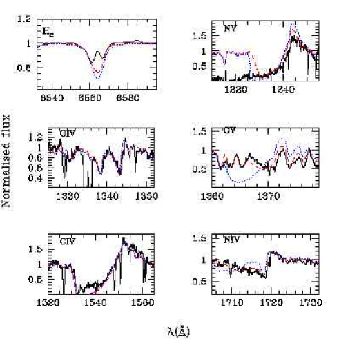
Figure 41: Influence of clumping on the determination of $\dot{M}$ of HD 93250. The solid line is the observed spectrum, the dotted line is a model with $\dot{M}$ = $10^{-5.46}$ M_⊙ yr^-1(mass loss rate derived by Repolust et al. repolust (2004) from H$\alpha$) and no clumping, and the dashed line is a model with $\dot{M}$ = $10^{-6.25}$ M_⊙ yr^-1and $f_{\infty}=0.01$. The inclusion of clumping leads to a reduction of the mass loss rate derived from both UV lines and H$\alpha$. See text for discussion.

Can we estimate the value of the slope of the WLR in this low $L$ range? The number of stars studied is still too low to give a reliable value, but if we do a simple by eye estimate, excluding star HD 152590 (due again to the fact that it is a possible member of a binary), we find a slope of the order of 4.3. As this slope is in fact equal to 1/$\alpha^{\prime}$ (e.g. Kudritzki & Puls kp00 (2000)), where $\alpha^{\prime}=\alpha-\delta$ and $\delta=0.005..0.1$, we deduce $\alpha^{\prime}\sim 0.25$ and $\alpha\sim 0.30$ which is very low compared to the classical value of $\sim$ 0.6, but which is consistent with our finding based on the ratio of terminal to escape velocities (Sect. 7.2.1). This does not mean that $\alpha$ is indeed this low for these stars since both $v_{\infty}$ and $\dot{M}$ may be underestimated, but it is at least a kind of consistency check.

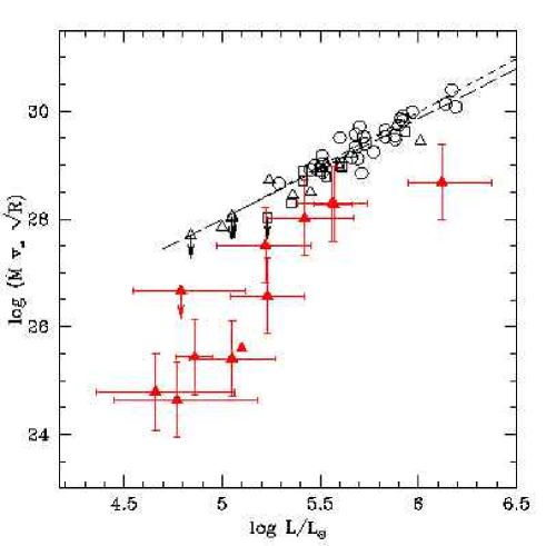
Figure 42: WLR for Galactic stars. Symbols and data are the same as in Fig. 39. Note the breakdown of the relation below $\log\frac{L}{L_{\odot}}\sim 5.2$. See text for discussion. The short (long) dashed line is the regression curve for supergiants (giants + dwarfs) of Repolust et al. (repolust (2004)).

7.2.3 Origin of weak winds

In view of the above results, what can we conclude as regards the origin of the weakness of the winds observed in some O dwarfs? The main possibilities have been detailed in paper I. Among them, metallicity was the first to come to mind since at that time, as most stars with weak winds were found in the SMC (paper I, Bouret et al. jc03 (2003)). The present study clearly shows that metallicity cannot explain the reduced wind strength observed since several Galactic stars show mass loss rates and terminal velocities as low as SMC objects. On the contrary, it becomes more and more evident that there is a transition in the wind properties near $\log\frac{L}{L_{\odot}}=5.2$, although the reasons for such a change of behaviour remain unclear at present. To say things more clearly, we do not state that metallicity has no effect on the wind strength (this is now well established): we simply show that low luminosity dwarf O stars have winds much weaker than expected from hydrodynamical simulations and than so far observed for O stars, independent of metallicity.

A possible explanation is the reduction of the $\alpha$ parameter which, if it were as low as $\sim$ 0.25, could explain both the reduced mass loss rates and terminal velocities. However, what could be the reason for such a low $\alpha$ ? A nice possibility was highlighted by Puls et al. (psl00 (2000)) in their very detailed analysis of the line statistics. They first show that under fairly general conditions, the classical $\alpha$ parameter, i.e. the one entering the slope of the line strength distribution function, and the $\hat{\alpha}$ parameter used to express the radiative acceleration according to

$$g^{rad}\propto t^{-\hat{\alpha}}$$ (10)

in the CAK formalism (see Castor, Abbott & Klein cak (1975)) are the same (this is the basics of the radiation driven wind formalism). However, the line strength distribution function may not have a constant slope, and in that case the value of $\alpha$ such that $\hat{\alpha}=\alpha$ must be derived at the point where the line strength is equal to $t^{-1}$. This has two important consequences: first, since $t=s_{e}v_{th}\frac{\rho}{dv/dr}$ (with $s_{e}$ the Thomson scattering opacity and $v_{th}$ the typical thermal velocity), it will be different from star to star; and second, $t$ is not constant in a given star’s atmosphere. In practise, this means that $\alpha$ should be different not only from star to star, but also from point to point in the atmosphere of a given star! However, Puls et al. (psl00 (2000)) have shown that the slope of the line strength distribution function is constant over a large range of $t$ values, implying that $\alpha$ keeps a constant value close to 0.6. But in extreme cases, we may reach a range where this slope varies: in that case, $\alpha$ is reduced. This is shown by Fig. 27 of Puls et al. (psl00 (2000)) where we see that for $t$ lower than 10^-6 $\alpha$ deviates significantly from 0.6. The interesting thing is that this situation corresponds to low densities (see the definition of $t$ above). In conclusion, $\alpha<0.6$ is expected in low density winds, which is consistent with our findings.

Given this fact, the main problem would come from the strong disagreement between the results of spectroscopic analysis and the predictions of hydrodynamical simulations. Could such simulations overestimate mass loss rates? It is indeed possible since they neglect velocity curvature terms in the computation of radiative accelerations (Owocki & Puls op99 (1999)), which can affect the final results. As discussed in paper I, O dwarfs with low luminosity are the most sensitive to such effects but test models for a 40 M_⊙ star performed by Owocki & Puls (op99 (1999)) lead to downward revision of the mass loss rate by only a factor 1.5 while we would need a factor $\sim$ 100!

One can also wonder what is the effect of X-rays on the driving of winds. We have already seen in Sect. 7.2.1 that low terminal velocities can be expected when X-rays are present due to changes in the outer atmosphere ionisation structure. Further insights can be found in Drew et al. (drew94 (1994)). These authors have studied two B giants and have found mass loss rates 5 times lower than values expected for a simple extrapolation of the $\dot{M}$ - $L$ relation of Garmany & Conti (gc84 (1984)) established for O stars. They also detected X-ray emission in both stars, and argued that such X-rays, likely formed in the outer atmosphere, can propagate towards the inner atmosphere and change the ionisation structure here too, reducing the total radiative acceleration and thus the mass loss rate. This may partly explain why the mass loss predictions of Vink et al. (vink01 (2001)), which does not take X-rays into account, are higher than our derived values. Obviously, hydrodynamical models including X-rays are needed to test this attractive hypothesis.

We highlighted in paper I that decoupling may be an alternative explanation although no conditions for it to take place were fulfilled in the N81 atmospheres. Here, the stellar and wind parameters of the weak winds stars being similar to those of the N81 stars, we have checked that such a process is not likely to be at work either.

8 Conclusion

We have derived the stellar and wind properties of Galactic O dwarfs with the aim of tracking the conditions under which weak winds such as observed in SMC-N81 (Martins et al. n81 (2004)) develop. Atmosphere models including non-LTE treatment, spherical expansion and line-blanketing were computed with the code CMFGEN (Hillier & Miller hm98 (1998)). Optical H and He lines provided the stellar parameters while both UV lines and H$\alpha$ were used to determine the wind properties. The main results can be summarised as follows:

• The O dwarfs studied here are 1 to 2 Myrs old for the hottest and 2 to 4 Myrs old for the coolest. Except for the faintest, they have luminosities in reasonable agreement with the new calibration $T_{\mathrm{eff}}$ - Luminosity of Martins et al. (calib05 (2005)).

• Stars with luminosities below a certain transition luminosity ($\log\frac{L}{L_{\odot}}\la 5.2$) have mass loss rates of the order of 10^-8..-9.5 M_⊙ yr^-1 and low terminal velocities (down to 800 km s^-1). The mass loss rates are lower by nearly a factor of 100 compared to the hydrodynamical predictions of Vink et al. (vink01 (2001)). Uncertainties in the determination of $\dot{M}$, discussed here in detail, are not expected to qualitatively alter the results.

• Stars with $\log\frac{L}{L_{\odot}}\ga 5.2$ are found to have reduced mass loss rates compared to both hydrodynamical predictions and previous analysis based only on H$\alpha$. The main reason is the inclusion of clumping in our models in order to fit O v $\lambda$1371 and N iv $\lambda$1718 in the IUE range. The adoption of pure H$\alpha$ based mass loss rates does not allow fits of most of the UV lines.

• The modified wind momentum - luminosity relation shows a break down around $\log\frac{L}{L_{\odot}}=5.2$. Below this transition value, the slope corresponds to a value of the $\alpha$ parameter of the order of 0.3, which is consistent with the low terminal velocities observed. Such a low $\alpha$ is expected in low density winds (Puls et al. psl00 (2000)).

• The origin of the weakness of the winds in low luminosity stars compared to hydrodynamical simulations is still unknown, but metallicity effects can be excluded since all the stars of the present study are Galactic stars and show reduced winds similar to SMC stars (Bouret et al. jc03 (2003), Martins et al. n81 (2004)). An earlier evolutionary state than in standard dwarfs may be responsible or not for the weakness: the present results can not resolve this issue given the error bars in the age estimates.

• Although their origin remains unclear, X-rays appear to play a very important role in the physics of weak winds. They may be due to magnetic mechanisms and affect the ionisation structure. This can possibly reduce the driving force and partly explain the low terminal velocities and low mass loss rates. Hydrodynamical simulations including X-rays should give more quantitative results.

The low luminosity objects of our sample have not been studied individually with quantitative spectroscopy before since the atmosphere models allowing the analysis of weak wind stars have only been available for a few years. Indeed, the detailed modelling of UV wind sensitive lines requires a reliable treatment of line-blanketing since most of these lines are from elements heavier than He. This also explains why a number of previous quantitative analysis relied essentially on H$\alpha$.

Now that the existence of weak winds has been established observationally both in the SMC and in the Galaxy, it would certainly be suitable to investigate the problem from a theoretical point of view with new hydrodynamical simulations. Apart from that, we still have to make sure that the ionisation fractions predicted by CMFGEN are correct since thay may alter the mass loss rate determinations. We will conduct such an investigation in a forthcoming paper using FUSE data.

- (1) Abbott, D.C., 1982, ApJ, 259, 282
- (2) Allen, C.W., 1976, Astrophysical Quantities, (London: Athlone)
- (3) Asplund, M., 2004, A&A. 417, 751
- (4) Auer, L.H. & Mihalas, D., 1972, ApJS, 24, 193
- (5) Babel, J. & Montmerle, T., 1997, ApJ, 485, L29
- (6) Bernabeu, G., Magazzù, A. & Stalio, R., 1989, A&A, 226, 215
- (7) Bouret, J.C., Lanz, T., Hillier, D.J., Heap, S.R., Hubeny, I., Lennon, D.J., Smith, L.J., Evans, C.J., 2003, ApJ, 595, 1182
- (8) Bouret, J.C., Lanz, T., Hillier, D.J., 2005, A&A, in press, astro-ph/0412346
- (9) Cassinelli, J.P. & Olson, G.L., 1979, ApJ, 229, 304
- (10) Castor, J., Abbott, D.C., Klein, R., 1975, ApJ, 195, 157
- (11) Chiosi, C. & Maeder, A., 1986, ARA&A, 24, 329
- (12) Chlebowski, T. & Garmany, C.D., 1991, ApJ, 368, 241
- (13) Cohen, D.H., de Messières, G., MacFarlane, J.J., Miller, N.A., Cassinelli, J.P., Owocki, S.P., Liedahl, D.A., 2003, ApJ, 586, 495
- (14) Crowther, P.A., Hillier, D.J., Evans, C.J., Fullerton, A.W., De Marco, O., Willis, A.J., 2002, ApJ, 579, 774
- (15) DeGioia-Eastwood, K., Throop, H. & Walker, G., 2001, ApJ, 549, 578
- (16) Donati, J.F., Babel, J., Harries, T.J., Howarth, I.D., Petit, P., Semel, M., 2002, MNRAS, 333, 55
- (17) Drew, J.E., Denby, M., Hoare, M.G., 1994, MNRAS, 266, 917
- (18) Evans, N.R., Seward, F.D., Krauss, M.I., Isobe, T., Nichols, J., Schlegel, E.M., Wolk, S.J., 2003, ApJ, 589, 509
- (19) Evans, C.J., Crowther, P., Fullerton, A.W., Hillier, D.J., 2004, ApJ, 610, 1021
- (20) Gagné, M., Oksala, M.E., Cohen, D.H., Tonnesen, S.K., Ud-Doula, A., Owocki, S.P., Townsend, R.H.D., MacFarlane, J.J., 2005, ApJ, submitted (astro-ph/0504296)
- (21) Garmany, C.D. & Conti, P.S., 1984, ApJ, 284, 705
- (22) Garmany, C.D. & Stencel, R.E., 1992, A&AS, 94, 211
- (23) Gieseking, F, 1982, A&AS, 49, 673
- (24) Grevesse, N. & Sauval, A., 1998, Space Sci. Rev, 85, 161
- (25) Grigsby, J.A., Morrison, N.D. & Anderson, L.S., 1992, ApJS, 78, 205
- (26) Haser, S.M., 1995, PhD thesis, Universitts-Sternwarte der Ludwig-Maximillian Universitt, Mnchen
- (27) Herrero, A., Puls, J., Villamariz, M.R., 2000, A&A, 354, 193
- (28) Herrero, A., Puls, J., Najarro, F., 2002, A&A, 396, 949
- (29) Hillier, D.J. & Miller, D.L., 1998, ApJ, 496, 407
- (30) Hillier, D.J., Lanz, T., Heap, S.R., Hubeny, I., Smith, L.J., Evans, C.J., Lennon, D.J., Bouret, J.C., 2003, ApJ, 588, 1039
- (31) Hiltner, W.A., 1956, ApJS, 2, 389
- (32) Hoogerwerf, R., de Bruijne, J.H.J. & de Zeeuw, P.T., 2001, A&A, 365, 49
- (33) Howarth, I. & Prinja, R.K., 1989, ApJS, 69, 527
- (34) Howarth, I.D., Siebert, K.W., Hussain, G.A.J., Prinja, R.K., 1997, MNRAS, 284, 265
- (35) Hubeny, I. & Lanz, T., 1995, ApJ, 439, 875
- (36) Humphreys, R.M., 1978, ApJS, 38, 309
- (37) Kendall, T.R., Lennon, D.J., Brown, P.J.F, Dufton, P.L., 1995, A&A, 298, 489
- (38) Klein, R.I. & Castor, J.I., 1978, ApJ, 220, 902
- (39) Kramer, R.H., Cohen, D.H., Owocki, S.P., 2003, ApJ, 592, 532
- (40) Kudritzki, R.P., Pauldrach, A., Puls, J., Abbott, D.C., 1989, A&A, 219, 205
- (41) Kudritzki, R.P., Lennon, D.J., Puls, J., 1995, in “Science with the VLT”, Proc. of the ESO workshop held at Garching, Germany, 28 June - 1 July 1994, Eds J.R. Walsh & I.J. Danziger, Berlin, Springer-Verlag, p. 246
- (42) Kudritzki, R.P., 1998, in “Stellar astrophysics in the Local Group: first step to the Universe”, Proc of the 8th Canary Island winter school, Eds. A. Herrero, A. Aparicio, F. Sanchez, Cambridge University press
- (43) Kudritzki, R.P., Puls, J., Lennon, D.J., Venn, K.A., Reetz, J., Najarro, F., McCarthy, J., 1999, A&A, 350, 970
- (44) Kudritzki, R.P. & Puls, J., 2000, ARA&A, 38, 613
- (45) Lamers, H.J.G.L.M., Cerruti-Sola, M., Perinotto, M., 1987, ApJ, 314, 726
- (46) Lamers, H.J.G.L.M. & Leitherer. C., 1993, ApJ, 412, 771
- (47) Lamers, H.J.G.L.M., Snow, T.P. & Lindholm, D.M., 1995, ApJ, 455, 269
- (48) Lamers, H.J.G.L.M. & Cassinelli, J.P., 1998, in “From Stars to Galaxies: the impact of stellar physics on Galaxy evolution”, ASP conf. series 98, eds. C. Leitherer, U. Fritze-Von Alvensleben & J. Huchra, p. 162
- (49) Lamers, H.J.G.L.M., Haser, S., de Koter, A., et al., 1999, ApJ, 516, 872
- (50) Lanz, T. & Hubeny, I., 2002, ApJS, 146, 417
- (51) Leitherer, C., 1988, ApJ, 326, 356
- (52) Lejeune, T. & Schaerer, D., 2001, A&A, 366, 538
- (53) Lucy, L.B. & Solomon, P.M., 1971, ApJ, 159, 879
- (54) Lucy, L.B. & White, 1980, ApJ, 241, 300
- (55) MacFarlane, J.J., Cohen, D.H., Wang, P., 1994, ApJ, 437, 351
- (56) Maíz-Apellániz, J., Walborn, N.R., Galué, H.Á., Wei. L.H., 2004, ApJS, 151, 103
- (57) Markova, N, Puls, J., Repolust, T., Markov, H, 2004, A&A, 413, 693
- (58) Martins, F., Schaerer, D., Hillier, D.J., 2002, A&A, 382, 999
- (59) Martins, F., Schaerer, D., Heydari-Malayeri, M., in “A massive star odyssey: from main sequence to supernova”, eds K.A. van der Hucht, A. Herrero, C. Esteban , IAU symp. 212, p. 564
- (60) Martins, F., Schaerer. D., Hillier, D.J., Heydari-Malayeri, M., 2004, A&A, 420, 1087 (paper I)
- (61) Martins, F., Schaerer, D., Hillier, D.J., 2005, A&A, 436, 1049
- (62) Massa, D., Fullerton, A.W., Sonneborn, G., Hutchings, J.B., 2003, ApJ, 586, 996
- (63) Massey, P., DeGioia-Eastwood, K., Waterhouse, E., 2001, ApJ, 421, 1050
- (64) Mason, B.D., Gies, D.R., Hartkopf, W.I., Bagnuolo, W.G., Brummelarr, T.T., McAlister, H.A., 1998, ApJ, 115, 821
- (65) Nicolet, B, 1978, A&AS, 34, 1
- (66) Pellerin, A., Fullerton, A.W., Robert, C., et al., 2002, ApJS, 143, 159
- (67) Milne, E.A., 1926, MNRAS, 86, 459
- (68) Olson, G.L., 1982, ApJ, 255, 267
- (69) Owocki, S.P., Castor, J.I., Rybicki, G.B., 1988, ApJ, 335, 914
- (70) Owocki, S.P. & Puls, J., 1999, ApJ, 510, 355
- (71) Pauldrach, A., Puls, J., Kudritzki, R.P., 1986, A&A, 164, 86
- (72) Pauldrach, A.W.A., Kudritzki, R.P., Puls, J., et al., 1994, A&A, 283, 525
- (73) Pauldrach, A.W.A., Hoffmann, T.L., Lennon, M., 2001, A&A, 375, 161
- (74) Pilyugin, L.S., Ferrini, F., Shkvarun, R.V., 2003, A&A, 401, 557
- (75) Penny, L. R., 1996, ApJ, 463, 737
- (76) Prinja, K.R., Barlow, M.J. & Howarth, I.D., 1990, ApJ, 361, 607
- (77) Puls, J., Kudritzki, R.P., Herrero, A., et al., 1996, A&A, 305, 171
- (78) Puls, J., Springmann, U., Lennon, M., 2000, A&AS, 141, 23
- (79) Puls, J., Urbaneja, M. A., Venero, R., Repolust, T., Springmann, U., Jokuthy, A., Mokiem, M.R., 2005, A&A, submitted
- (80) Raymond, J.C. & Smith, B.W., 1977, ApJS, 35, 419
- (81) Repolust, T., Puls, J., Herrero, A., 2004, A&A, 415, 349
- (82) Rolleston, W.R.J., Smartt, S.J., Dufton, P.L., Ryans, R.S.I., 2000, A&A, 363, 537
- (83) Santolaya-Rey, A.E., Puls, J. & Herrero, A., 1997, A&A, 323, 488
- (84) Schild, R.E., Garrison, R.F., Hiltner, W.A., 1983, ApJS, 51, 321
- (85) Schulz, N.S., Canizares, C., Huenemoerder, D., et al., 2003, ApJ, 595, 365
- (86) Schmidt-Kaler, T., 1982, in Landoldt-Brnstein, New Series, Group, VI, Vol.2, eds. K. Schaifers & H.H. Voigt (Berlin: Srpinger-Verlag), 1
- (87) Schulz, N.S., Canizares, C., Huenemoerder, D., Tibbets, K., 2003, ApJ, 595, 365
- (88) Smartt, S.J., Venn, K.A., Dufton, P.L., Lennon, D.J., Rolleston, W.R.J., Keenan, F.P., 2001, A&A, 367, 86
- (89) Ud’Doula, A. & Owocki, S.P., 2002, ApJ, 576, 413
- (90) Vacca, W.D., Garmany, C.D. & Shull, J.M., 1996, ApJ, 460, 914
- (91) van Rensbergen, W., Vanbeveren, D., de Loore, C., 1996, A&A, 305, 825
- (92) Villamariz, M.R., Herrero, A., Becker, S.R., et al., 2002, A&A, 388, 940
- (93) Vink, J., de Koter, A. & Lamers, H.J.G.L.M., 2000, A&A, 362, 295
- (94) Vink, J., de Koter, A. & Lamers, H.J.G.L.M., 2001, A&A, 369, 574
- (95) Walborn, N. & Parker, J., 1992, ApJ, 399, L87
- (96) Walborn, N., Nichols-Bohlin, J., Panek, R.J., 1985, IUE Atlas of O-Type stellar spectra, NASA RP 1155
- (97) Walborn, N.R., Howarth, I.D., Lennon, D.J., Massey, P., Oey, M.S., Moffat, T., Skalkowski, G., Morrell, N.I., Drissen, L., Parker, J.W., 2002, AJ, 123, 2754