Investigation of flat spectrum radio sources by the interplanetary scintillation method at 111 MHz.

Interplanetary scintillation observations of 48 of the 55 Augusto et al. (1998) flat spectrum radio sources were carried out at 111 MHz using the interplanetary scintillation method on the Large Phased Array (LPA) in Russia. Due to the large size of the LPA beam ($1\degr\times 0.5\degr$) a careful inspection of all possible confusion sources was made using extant large radio surveys: 37 of the 48 sources are not confused. We were able to estimate the scintillating flux densities of 13 sources, getting upper limits for the remaining 35. Gathering more or improving extant VLBI data on these sources might significantly improve our results. This proof-of-concept project tells us that compact ($<1^{\prime\prime}$) flat spectrum radio sources show strong enough scintillations at 111 MHz to establish/constrain their spectra (low-frequency end).

1 Introduction

A systematic search for dominant structure on 0.09–0.3^′′ scales in large flat-spectrum radio source samples was made by Augusto et al. (Augusto98 (1998)). Fifty-five radio sources were selected from a parent sample containing 1665 strong flat-spectrum radio sources ($S_{8.4\leavevmode\nobreak\ GHz}>100$ mJy; $\alpha_{1.4}^{4.85}<0.5,S_{\nu}\propto\nu^{-\alpha}$). These sources all have published MERLIN 5 GHz data. A few also have VLBA 5 GHz and MERLIN 22 GHz maps (Augusto et al. Augusto98 (1998)). In addition, some others have MERLIN+EVN 1.6 GHz high angular resolution ($<0.5^{\prime\prime}$) unpublished data (Augusto et al., in prep.).

The study of these 55 sources is not complete without low frequency observations ($\sim 100$ MHz), as was pointed out in Augusto et al. (Augusto98 (1998)), where the spectra of most sources have no data at all below $\sim 300$ MHz. The turnovers in the spectra of compact components in these sources must be found, to give a physical meaning to all 55 sources, namely by fitting synchrotron emission spectra for them all. Since VLBI does not routinely (or efficiently) operate at such low frequencies, we use the interplanetary scintillation (IPS) method at 111 MHz with the Large Phased Array (LPA). Very similar work was done at LPA for compact steep spectrum sources (Artyukh et al. Artyukh99 (1999); Tyul’bashev & Chernikov Tyulbashev00 (2000), Tyulbashev01 (2001)). The principle of IPS is very simple: the solar wind has variations in electron density on which depends the velocity of the radio waves that travel through it. As a result, we have a phase screen which can increase or decrease the signal from distant radio sources; i.e. the sources will scintillate. The characteristic time of scintillations depends on the velocity of the solar wind, on the frequency of the observations, and on the sizes of the electron clouds. For example, if we have observations at 111 MHz, this characteristic time scale is approximately one second. The scintillations will be stronger if the distant radio sources (or components therein) have small angular sizes ($<1^{\prime\prime}$). Details of observations by the IPS method and relevant theory can be found, for example, in Vlasov et al. (Vlasov79 (1979)).

The IPS method has advantages and disadvantages when compared with VLBI observations. The main advantage is the possibility to observe sources at low frequencies and high resolution. The main disadvantage is the very low positional accuracy. We see scintillations, but we do not know exactly which component(s) is(are) scintillating or even if we correctly identify the main radio source (among many in-beam): the coordinate uncertainties for LPA are 5-10^s in right ascension and 2-3^′ in declination for strong sources ($\sigma_{scint}/\sigma_{noise}>2$, at $\tau=0.5$ s; standard SNR $>7$), increasing to 30-60^s and 5-7^′, respectively, for weak sources ($\sigma_{scint}/\sigma_{noise}<2$). These uncertainties have a complex behaviour ($f(\sigma_{scint},\sigma_{noise}$); Artyukh & Tyul’bashev Artyukh96 (1996)). In order to get around these large, inherent errors (i.e. to, at least, correctly identify the source with the scintillating component) for all pointings that we have done with the LPA, we extensively searched the entire beam area using both the 1.4 GHz NRAO VLA Sky Survey (NVSS; Condon et al. Condon98 (1998); www.cv.nrao.edu/nvss) and the 74 MHz VLA Low-Frequency Sky Survey (VLSS; lwa.nrl.navy.mil/VLSS). The whole of Sect. 3 is devoted to this study. In Sect. 2, we present both the data collection and reduction, while in Sect. 4 we compile the IPS 111 MHz results from observations of 48 of the 55 Augusto et al. (1998) sources, for which we derive either a scintillating flux density estimate (13) or an upper limit (35). We also include in this section, as a case study, the detailed spectrum analysis for B0821+394. Finally, a short discussion and summary is given in Sect. 5.

2 Observations and data analysis

We carried out 111 MHz IPS observations with the LPA (a meridian instrument) of the Lebedev Institute of Physics, Russia. The effective area of the antenna in the zenith direction is $2\times 10^{4}$ m² with a beam approximately $1\degr\times 0.5\degr$ (EW $\times$ NS) in size. The receiver integration time was $\tau=0.5$ s, the sampling time 0.1 s, and its bandwidth 600 kHz. As a result, the sensitivity of LPA for scintillating sources is $\sigma_{scint}\simeq$0.15–0.2 Jy in the zenith direction (with s.n.r. $\geq 10$, after the integration of all scintillations), decreasing with source declination as $\cos(\delta)$, where $\delta$ is the declination of the source. The r.m.s. confusion due to extended (nonscintillating) sources is $\sim$1 Jy, while the r.m.s. confusion due to scintillating sources is $\leq$ 0.12 Jy. This means that even when it is difficult to measure the total flux density of a source, it is still possible to measure the scintillating flux density.

We carried out 137 sessions in 2001-2002, each with a duration between 5 and 11 hours. We observed, in each session, from 5 to 10 calibrators and always less than 15 target sources. Thus, a total of between 20 and 25 individual records were gathered per session and all targets were observed in more than one run ($N$ on Column (2) of Table 3). The integration time for each source depended on its declinitaion, so it varied from approximately 9 to 18 minutes. In total, we had over 1100 hrs of observation time, half of which on-target. Many individual source observations had to be prolonged to compensate for interference. Due to the large number of sources, it was not possible to choose the best elongation for each source as it was done in Artyukh (Artyukh81 (1981)). Therefore, we used the converting coefficients of Marians (Marians75 (1975)). We also selected the best data: the records, among the many observed, with the lowest noise.

Flat spectrum sources are very difficult to detect at low frequencies (in total flux density), therefore the data reduction must be made with care (c.f. similar steep-spectrum radio source analysis in Tyul’bashev& Chernikov Tyulbashev01 (2001)). The data reduction method we used is given in Artyukh (Artyukh81 (1981)) and Artyukh & Tyul’bashev (Artyukh96 (1996)). This method enables us to detect faint scintillating sources, for which the scintillation dispersion ($\sigma_{scint}^{2}$) is smaller than the noise (dispersion) on the receiver time constant $\tau$. We estimate this noise in the parts of the data record where we cannot see scintillations, i.e., where the noise seen is minimal. The accuracy of the scintillating flux density estimate ($S_{compact}\equiv S_{c}$) depends on the fluctuation of the flux density ($\sigma_{scint}$) and on the elongation of the source (angle between the Sun and source directions as seen by the observer). The typical accuracy is 20-25% for elongations smaller than $40\degr$ and ($\sigma_{scint}$) higher than the noise of the antenna in a given direction. In the worst cases, the accuracy of $S_{c}$ estimates is still better than 30-50% (see details in Artyukh & Tyul’bashev Artyukh96 (1996); Artyukh et al. Artyukh98 (1998)).

Our observations lead to two situations: i) the compact source/components is/are too weak; no scintillations are detected but we can place an upper limit on the scintillation flux density ($S_{c}$); ii) scintillations are seen from a compact component in the source. We try to get the best possible estimate of $S_{c}$ by combining all existing (good) records (column (2) of Table 3). The individual (statistical) error of a single record is 5–7%, hence combining them decreases it. Unfortunately, this error is overwhelmed by the calibration error at LPA (10–20%).

In what follows we summarize the observing/data reduction steps for each source (see also Sect. 4.2):

1. We observe one (or more) flux density calibrator(s) — several records.

2. We observe the target source (several records).

3. If possible, we estimate the total flux density ($S_{t}$) using the calibrator and target records. $S_{t}$ adds the scintillating flux density (compact component(s)) and the non-scintillating one (extended component(s)).

4. We look for scintillations in the target record by first removing the background and then pulse interferences, having only noise left (instrumental — $\sigma_{noise}$ — and scintillating — $\sigma_{scint}$). Then, we split these noises from the fact that $\sigma_{noise}$ exists all the time, while $\sigma_{scint}$ exists only from a given direction — primary record.

5. It is this latter part (few minutes) of the main record that is used to estimate $S_{c}$ using $\sigma_{scint}$ and information on the angular sizes of the source and its components (e.g. Marians Marians75 (1975)).

3 Confusion analysis

The fact that the LPA has a huge beam ($1.0\degr\times 0.5\degr$) makes it imperative that we clearly identify the source that includes the component actually scintillating at 111 MHz. It might not be the main source (as listed in Table 3) since many other radio sources exist inside the LPA beam and might cause confusion due to producing stronger scintillations. Ideally, we should have available VLBI maps for all compact (and fairly strong) sources inside each of the LPA pointings. There is no such survey available at high frequencies and even fewer at 111 MHz. Hence, the best we can do is to use existing literature and non-VLBI survey information in order to guess the source where the scintillating component lies. The best surveys to date that could suit our purposes used the VLA-A at 8.4 GHz (0.2″resolution): the Jodrell-VLA Astrometric Survey (JVAS; e.g. Patnaik et al. Patnaik92 (1992)) and the Cosmic Lens All-Sky Survey (CLASS; e.g. Myers et al. Myers03 (2003)). Apart from the main sources, which all have VLA-A 8.4 GHz compact components, only four “candidates” were detected by those surveys (see below).

There are three surveys of interest to our study. Although with much lower resolution than JVAS/CLASS, they were made at lower frequencies. The most relevant of these, at least as regards the frequency of observation, is the VLSS done with the VLA (B and BnA) at 74 MHz (80″resolution). It certainly can identify the strongest sources in each of our LPA pointings but, unfortunately, it cannot tell us much about compactness. Another useful survey is the Faint Images of the Radio Sky at Twenty-centimeters (FIRST — Becker, White & Helfand Becker95 (1995); sundog.stsci.edu/top.html), done with the VLA-B at 1.4 GHz (5″resolution). Its resolution, altough still three orders of magnitude above VLBI scales, is 16 times better than the one of VLSS, but the shift to high frequencies does not help much in our study. Unfortunately, both of the previous surveys lack full-sky coverage. The VLSS is still on-going, while FIRST covers less than half of the northern sky, where all our sources lie. As a result, out of the 48 pointings done with the LPA (centred on each of the main sources), 34 (71%) fell inside the VLSS sky coverage while only 19 (40%) are in FIRST. The last survey we used in our study is the NVSS, made with the VLA (D and DnC) at 1.4 GHz (45″  resolution), which covers the full northern hemisphere; hence, it should contain all candidates to confusing sources of our observations.

Our “candidate-finding” scheme was to fully examine a $1.0\degr\times 0.5\degr$ area (equal to the LPA beam), centred on our main source position, using the Internet search engines in VLSS, NVSS, FIRST, and NED (the NASA Extragalactic Database; nedwww.ipac.caltech.edu), in order to get extra literature information (namely radio spectra and maps), if any. This has found a total of 1046 candidates for the 48 sources or ‘pointings’ ,the vast majority quite weak (Appendix A). All of these are in the NVSS, but only 271 (out of the surveyed total of 378 — 72%) and 29 (total 736, so 4%) are detected in FIRST (S${}_{1.4}\ga 1$ mJy/beam) and VLSS (S${}_{74}\ga 0.5$ Jy/beam), respectively. A total of 135 candidates are in both surveyed areas, bringing the grand total of candidates with more information than NVSS-only to 979, so only 67 (7%) lack it. Three candidates have only non-FIRST maps available while 36 others have only radio spectra as extra information: there are 82 candidates with spectral information of which 27 also have radio maps (see Table 1). The question now is: How do we know if a candidate is strongly scintillating or not at 111 MHz? Obviously, the seven sources of Table 1 with high resolution information (of which four also have FIRST maps) are the only ones for which the best guess can be made. These are described, individually, in what follows:

J0117+321:

In JVAS (e.g. Wilkinson et al. Wilkinson98 (1998)), this source shows up as compact ($<0.2\arcsec$). However, it is a GPS source and can be ruled out as candidate since it is likely too weak at low frequencies.

J0823+391:

Also in FIRST (resolved; $\sim 30\arcsec$ wide large symmetric object with two edge-brightened lobes; 62 mJy/beam), this had further VLA observations done by Lehar et al. (Lehar01 (2001)) which show one of the lobes resolved ($\sim 1\arcsec$ in size), the other compact ($<0.7\arcsec$; 4 mJy/beam), as well as a central core ($<0.7\arcsec$; $<1$ mJy/beam). It might contain VLBI compact components, but is possibly too weak to cause confusion; on this basis, we rule it out.

J0825+393:

In FIRST, it is a bright (1106 mJy/beam) unresolved source; mapped with VLBI, it looks like a compact (size $<0.07\arcsec$) steep spectrum source (Dallacasa et al. Dallacasa02 (2002)). A definitly confusing candidate that must be kept.

J1013+493:

A JVAS compact source ($<0.1\arcsec$ — e.g. Patnaik et al. Patnaik92 (1992)), it is actually a VLBI calibrator with a size $<0.02\arcsec$ (Beasley et al. Beasley02 (2002)). In FIRST it shows up as a bright (266 mJy/beam) unresolved source. A definitly confusing candidate that must be kept.

J1215+331A:

Also known as NGC4203, this source has a FIRST map available (slightly resolved; 6 mJy/beam). It very likely contains a central compact core ($<1\arcsec$) with an inverted spectrum, possibly due to free-free absorption (e.g. Falcke et al. Falcke00 (2000); Ho & Ulvestad Ho01 (2001)). It shows an inverted spectrum at high frequencies, most likely too weak at low frequencies to confuse our observations, so ruled out.

J2152+175:

A core-plus-one-sided-jet VLBI source (e.g. Fey & Charlot Fey97 (1997)), this source extends to very large structures becoming a narrow angle tailed large radio galaxy (Rector & Stoke Rector01 (2001)). Both compact ($<0.2\arcsec$) and extended components are also seen in a VLA-A 8.4 GHz map (e.g. Browne et al. Browne98 (1998)). Its spectrum has a ‘knee’ at $\sim 1$ GHz, possibly peaking at $\la 1$ MHz: a typical core+halo spectrum. A definitly confusing candidate that must be kept.

J2154+174:

Slightly resolved ($<0.01\arcsec$ size) with the VLBI (Beasley et al. Beasley02 (2002)) it is a VLA-A 8.4 GHz compact source ($<0.1\arcsec$; Browne et al. Browne98 (1998)). Its spectrum has a ‘knee’ at $\sim 1$ GHz, possibly peaking at $\sim 10$ MHz (core+halo). A definitly confusing candidate that must be kept.

As regards the remaining, to first order, the answer lies in the VLSS data. Only roughly half (15) of the 29 candidates are stronger than the respective main source, all lacking high resolution maps for compactness determinations. The question is, then, how to proceed? In what follows, we will use all existing information we can in order to guess the compactness of each.

Taking advantage of existent spectral information, we decided to use the spectral index value between VLSS and NVSS ($\alpha_{74}^{1400}$) of each candidate, as compared to the corresponding value of the main source (if existent), as indicative of the likelihood of a given candidate confusing the observations or not. If $\alpha_{74}^{1400}$ is steeper for the candidate than for the main source, we take it as likely to be more extended, less compact, and hence less probable of confusing our observations. Such comparison could be done for six of these 15 candidates, all rejected as confusing candidates. What about the remaining nine? One of them (with $\alpha_{74}^{1400}=1.0$) has no further information, but we rule it out due to the comparison with the $\alpha_{fit}\simeq 0.7$ overall 232–1400 MHz spectrum of the corresponding main source which, in addition, has a Giga-hertz Peaked Spectrum (GPS) core-like component at 1.4–8.4 GHz. Four other candidates do have proper spectral information and the direct comparison using $\alpha_{fit}$ rules them all out; three have power-law spectra while the corresponding main source has a spectrum with a ‘knee’, suggesting a halo+compact core source — so, in these cases, the candidates are not likely to confuse our observations (scintillations should come from the ‘core’ component in the main source). The last one, however, peaks at $\sim 100$ MHz, while the corresponding main source has a halo+core spectrum; hence, both sources might have compact components and we do not know which one is the stronger scintillator at 111 MHz. So, for caution, we keep it as confusion candidate.

What about the 14 candidates that are weaker than the main source? Although not confusing our observations, they might make some relevant contribution to the total scintillating flux density of the main source. Chasing their possible compactness properties, we use $\alpha_{74}^{1400}$ as above to rule out all but four candidates that must be kept in the group because of their flatter values. As a matter of fact, two of these candidates have high resolution maps available (see Table 1) confirming them with compact VLBI components.

The VLSS analysis is not yet complete, however: what about non-detections? Candidates in this situation must be ruled out only if the corresponding main source was indeed detected. Out of the 736 candidates surveyed by the VLSS, 683 (93%) are thus ruled out in three different situations: i) 277 (NVSS) candidates reside in the 19 VLSS ‘pointings’ that found no confusing candidates at all; ii) 356 candidates in the remaining 14 VLSS ‘pointings’ with a detected main source stronger than each of them; iii) 50 ‘control’ candidates, with FIRST and/or spectra information (six have both; see Table 1).

With the hope of making use of the extant FIRST/NVSS data for the 309 candidates left that were not surveyed by VLSS, we tried to define and calibrate criteria for ruling out candidates. For this, we used both the 50 ‘control’ candidates not detected in the VLSS and the 21 extra candidates in Table 1 that actually have both FIRST and radio spectra information (Appendix B) — six of the 27 candidates in Table 1 are included in the 50 ‘control’ candidates (N.D. in Column (7) of Table 1). This, however, was not possible, since both a combined classification and a separate one failed the calibration tests. Hence, since there is no strong statistical basis to rule out (or not) a candidate using FIRST and/or spectral information, being conservative, we keep all 333 remaining candidates, regardless of their extra information. In a final attempt to split this number into highest/lowest probabilities of confusing our observations, we used 1.4 GHz NVSS flux density information (c.f. Appendix A) to reason as follows: if a source is too weak, its spectrum would have to be too steep to reach ‘confusion levels’, i.e., to have a comparable low frequency flux density to the respective main source. This time, we must set an arbitrary limiting value: $\alpha=1.5$. Steeper candidates are rejected. Using, then, the lowest frequency (lo) with measured flux density for each respective main source (on 151–356 MHz), 262 candidates do not reach 20% of that value keeping $\alpha_{lo}^{NVSS}<1.5$ and are, thus, rejected. The 71 candidates left can be further split into 16 included in Table 2, with the highest probability of causing confusion (they reach main source flux densities within $\alpha_{lo}^{NVSS}<1.5$), and 53 other (in the fields of 14 main sources with “confused?” or “confused” in Column (10) of Table 3) which reach 20–100% of each low frequency main source flux densities within $\alpha_{lo}^{NVSS}<1.5$.

In Table 2 we present the final list of 23 high probability confusing candidates, corresponding to the 11 main sources signaled with “confused” in Column (10) of Table 3. Thus only about 23% of our observed sources might have a good probability of being confused. It is impossible to make any better statement based on extant data since, to some degree, all 48 sources might be confused. Only detailed VLBI observations of all 1046 candidates might establish definitive conclusions.

4 Results

4.1 Overall

The results of our observations are presented in Table 3. We observed 50 sources from the sample of 55 sources in Augusto et al. (1998) but only got scintillating flux density data for 48 (87% completeness): five sources have not been observed because of their high declinations ($\delta>70^{\circ}$), resulting in too poor elongations — B0205+722, B0352+825, B0817+710, B0916+718, B1241+735; two other (B0905+420 and B1003+174) were confused by nearby strong VLBI sources (B0904+417 and B1004+178, respectively), so no information about $S_{c}$ is available for these either.

The IPS method requires knowledge of the upper limit for the (at least; ideally the actual) size of the scintillating component of a radio source in order to measure its flux density accurately. We should gather as much size information as possible for all compact components of each (e.g. Artyukh et al. Artyukh99 (1999)). This was not possible for the 17 sources in Table 3 (35% of the total), indicated with a star ($\star$) after their names, for which either VLBI data are not available or there is still ambiguity in identifying the scintillating component: their $S_{c}$ should have their current uncertainties much reduced if/when those data are collected. For example, the source B1058+245 has three components Augusto et al. Augusto98 (1998). The two at northeast have angular sizes 0.062$\times$0.022″(A) and 0.103$\times$0.053″(B), and are separated by 0.047″. The southwest component has size 0.314$\times$0.094″(C), and is 0.8″away from the other two. Scintillations from all components will add simultaneously, combining their flux densities. Hence, we do not know which component(s) contributes most at 111 MHz, because we do not have spectral information for each component. If it is component A, we get S${}_{c}<$0.27Jy; if component C we get S${}_{c}<$0.5Jy. Thus, we put the value $<$0.5Jy (hoping to improve it in the future) in column (7) of Table 3.

When possible, we have thoroughly investigated the structure of each source from the published (high frequency) VLBI-maps (columns (4) and (5) in Table 3). We checked (when possible) whether the spectra of compact components are peaked at high frequencies. These components should not dominate at low frequencies and we excluded them from further consideration. We also excluded components which have less than five times the flux density of any other component. Among the remaining compact components, we tried to find those with a comparatively high flux density and steep spectrum at high frequencies and assumed that they have power-law spectra down to low-frequency. Such an analysis allows us to reveal one or several components of known angular size dominating at 111 MHz.

In Column (8) of Table 3 we show the total flux densities at 74 MHz from the VLSS while in Column (9) we present the $\alpha_{74}^{1400}$ spectral index with the help of the NVSS. Out of the 48 sources, 33 (69%) have, at least, some indication of flux density at 74 MHz (seven are below $5\sigma$), while only one (B0529+013) is not detected. The remaining 14 sources are not in the current VLSS sky coverage.

4.2 Case study: B0821+394

We have chosen B0821+394 as a case study because it demonstrates all features typical of scintillating sources. It has the strongest scintillation in our sample (column (7), Table 3), allowing us to even estimate $\sigma_{scint}$ ‘by eye’ from Fig. 1. It has enough total flux density to subtract the background. Finally, it has a lot of observations at high angular resolution, and therefore we can do an accurate analysis of its structure in order to guess which compact components will dominate at 111 MHz.

Figure 1: Primary record of the strong scintillating source B0821+394. The comparison between “scintillation+noise” and “noise” gives us the possibility of estimating pure scintillations. The details of reduction of such observations are, for example, in Artyukh & Tyul’bashev (Artyukh96 (1996)).

Our observations of B0821+394 were obtained during six days at elongations from $34^{\circ}$ to $46^{\circ}$ accumulating to a total of 105 minutes. The value of $\sigma_{scint}$ varied substantially from session to session of observations, therefore we have a large error (25%) in our estimation of $S_{c}$ — Table 3. With an even larger error we could measure its total flux density ($S_{t}$).

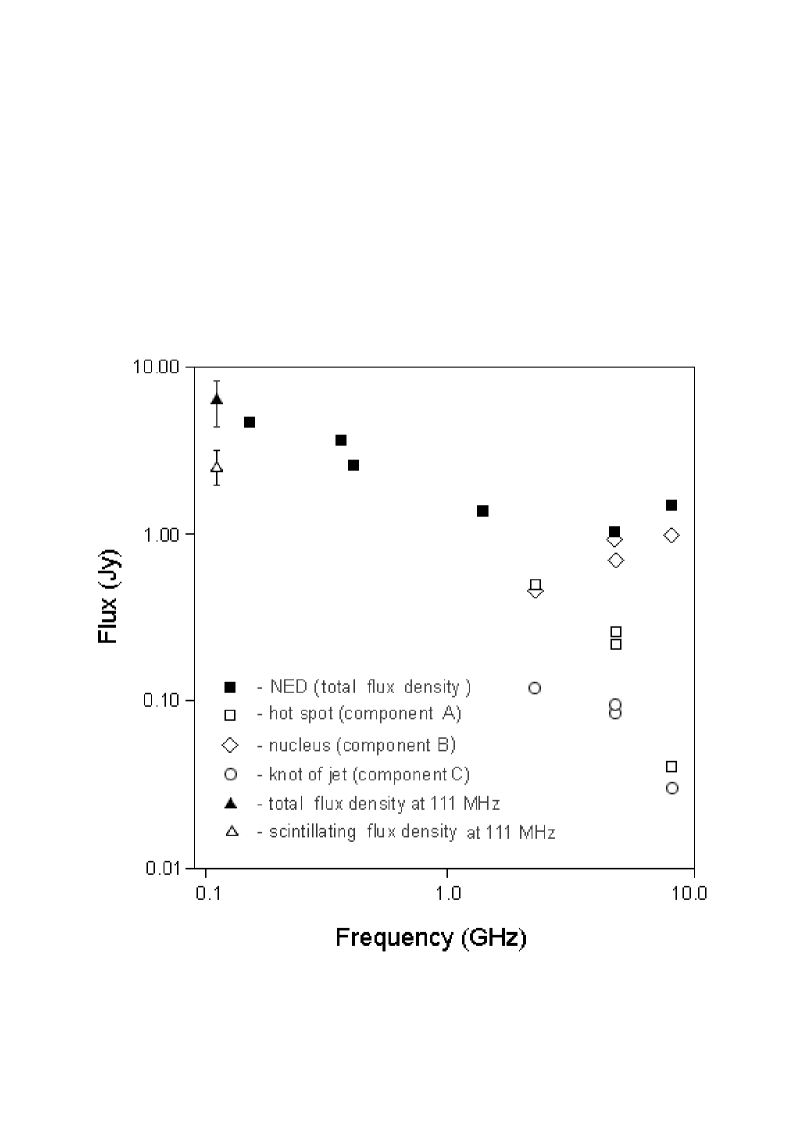
Figure 2: Spectrum of the source B0821+394 and spectra of its compact components (NED — NASA Extragalactic Database).

The radio source B0821+394 is a complicated SE-NW core-plus-one-sided-jet with redshift 1.216 (Wills & Wills Wills76 (1976); Augusto et al. 1998). This source has previously been observed with high angular resolution (1.6 GHz — MERLIN, 8.4 GHz — VLA-A, 5 GHz — VSOP; references in column (5) of Table 3) and from these data we can model it, to first order, with three main components: A) NW ‘hot spot’ with angular size $11\times 9$ milliarcseconds (mas) at p.a.$=-38^{\circ}$ and $\sim 250$ mas away from the nucleus; B) SE nucleus with size $<0.3\;\times<0.5$ mas; C) SE ‘knot’ (start of jet) with size $2\;\times<0.7$ mas at p.a.$=-18^{\circ}$, and $\sim 13$ mas away from the nucleus. Since components A, B, and C are so close and compact, B0821+394 will scintillate strongly from all, simultaneously. Hence, the flux densities of these compact components add to give the result in column (7) of Table 3. However, as we see next, only one of these components can dominate at 111 MHz. Building the spectra of components A, B, and C from information in the literature (Fig.2), we see that the nucleus (B) has a GHz-peaked spectrum (decreasing to low frequencies), while components A and C have power-law spectra. We have an overall flat spectrum source, as was previously known (Augusto et al. 1998). Our estimation of the total flux density ($6.5\pm 2$ Jy) agrees with other data while the scintillating flux density from components A and C is $2.5\pm 0.6$ Jy.

5 Discussion

In a sense, this paper is a proof-of-concept for the application of the IPS technique to flat-spectrum radio sources, which are expected to cause rather more difficulty in the estimation of total flux densities ($S_{t}$) at 111 MHz using such a method since they are, generally, much weaker (in S_t) than the steep-spectrum radio sources investigated earlier (Tyul’bashev& Chernikov Tyulbashev01 (2001)). We found that one-fourth (13 out of 48) of the flat-spectrum sources observed by us got estimates in $S_{c}$ that, in the worst scenario, have errors smaller than 35% (Table 3), with one exception at $<50\%$. We were even able to determine $S_{t}$ within 60% errors for the five strongest sources. How in the future can we improve our estimations of $S_{c}$? Simply by getting proper multi-frequency high resolution observations that might enable us to identify the scintillating component(s) at 111 MHz. This next step is well under way (Augusto et al., in prep.). As regards the 35 sources with upper limits (only), we might improve them substantially or, better, transform them into actual $S_{c}$ estimates, with the advent of high resolution data.

The previous results, however, had to be strengthened, due to the large LPA beam ($1\degr\times 0.5\degr$), by making sure that most targets were not affected by confusion. Due to the lack of more appropriate surveys, 1046 confusion candidates were identified by an extensive search in NVSS (surveying 100% of candidates), VLSS (70%), FIRST (36%), and NED. Of these, only seven (0.7%) have published high resolution maps (VLBI/VLA). It is tantalizing that 97% of the candidates residing in the VLSS 74 MHz surveyed areas (683 candidates, or 93% of the total number) were not detected ($S_{74}<0.5$ Jy/beam), while the respective targets were so, all but one; and out of the remaining 3% (29 candidates), using the steepness of $\alpha_{74}^{1400}$ (and VLBI maps for two) when compared with the corresponding main source, only five (17%) were not ruled out as causing confusion. Four other candidates were maintained thanks to detailed VLBI maps. Using detailed spectral information (for two) and VLA maps, three further candidates were ruled out. Finally, 262 extra candidates that cannot reach 20% of the main source low frequency (lo) flux density within $\alpha_{lo}^{NVSS}<1.5$ were ruled out; 53 that reach 20–100% are low probability confusion candidates while the remaining 16 join seven others from the map/spectra selection (Table 2) as the highest probability candidates for causing confusion: only 11 (23%) of the 48 main sources are thus affected.

As was pointed out in Augusto et al. (1998), 31 out of their 55 sources (56%) have no data below $\sim$300 MHz. The observations presented in this paper might be a breakthrough for establishing the low-frequency spectra of the 55 sources in Augusto et al. (1998), since 48 were observed, meaning 87% completeness. Relevant new information from our data comes from the estimates on $S_{c}$ at 111 MHz as compared with the total flux densities at 74/151 MHz from the literature (e.g. Augusto et al. 1998 and Table 3) — we can place an approximate upper limit on the flux densities of extended low surface brightness components, for the sources B0116+319 ($\la 0.4$ Jy), B0824+355 ($\la 1.5$ Jy), and B1211+334 ($\la 1.5$ Jy).

Knowledge of the low-frequency end of the radio spectrum of a radio source (and its components) is vital before fitting any synchrotron emission model to gain knowledge about its physical properties. Our objective, in due course, is to make such fits for all 55 sources. There is potential for all but one source since, in addition to the 48 presented in this paper, six out of the seven left out actually have 151 MHz total flux densities in the literature. Since these exist in two main types (core+(distorted)-jets; compact/medium symmetric objects — believed to be the precursors of large FRI/FRII radio galaxies), we think we can contribute to clarifying the origin of this subset of active galactic nuclei, at least as regards their emission mechanisms.

Appendix A The flux densities of the confusion candidates

As regards NVSS flux densities, out of the 1046 candidates, 950 (91%) have 1.4 GHz flux densities $<37$ mJy. This leaves 96 strong ($\geq 37$ mJy) candidates, of which 28 are also in the VLSS. It is tantalizing that, out of these 96 ‘strong’ candidates, only four, in three pointings, have NVSS 1.4 GHz flux densities stronger than the corresponding main source with flux density ratios 1.6, 1.1, 2.9 and 1.3, respectively.

For all three FIRST types [i) unresolved ($U$); ii) slightly resolved ($SR$); iii) resolved ($R$)] — see Appendix B, the weakest detected source has 1 mJy/beam. In Figure 3 we present the flux density distributions for each type. Comparing the flux density distributions up to S${}_{1.4}=15$ mJy/beam, we exclude 29% of unresolved sources, 14% of slightly resolved ones, and 19% of resolved sources. Going further down to S${}_{1.4}\leq 4$ mJy/beam, the respective exclusion rates are 65%, 45%, and 39%, thus showing a trend for the weakest sources to be resolved.

The comparison of the VLSS flux densities between the candidates and each corresponding main source is only possible for 13 pointings (out of 19), corresponding to 20 candidates (out of 29), since for the remaining there are no VLSS flux density measurements of the main source. Overall, the flux density ratios are in the range 0.2–4.1 with all but two candidates in the interval 0.4–2.6. Hence, the typical candidate-main source flux density ratio is within a factor of about 2.5.

Appendix B FIRST/spectral classification

As regards to the use of spectral information, in the hope of applying a similar spectral criterion to the one applied for the 29 VLSS candidates (Sect. 3), as before, depending on the number and range of the data points, we split the 60 candidates with spectral information into two large groups (usually the main source has more data points than each corresponding candidate and includes data at all available frequencies): two data points — group I — two-frequency spectral index calculation, compared with the same spectral index for the main source; three to five data points—group II — a linear regression is made (a global spectral index is fitted) and the result is compared with the one obtained by applying the same technique to the corresponding main source, using the same frequency range. Then, depending at which frequencies they have data, we split them further into the following seven subgroups (between brackets the number of candidates inside each subgroup) : Ia) 1.4–2.7 GHz (1); Ib) 1.4–4.85 GHz (8); Ic) (318 or 365 or 408) to 1400 MHz (27); Id) 151–1400 MHz (8); IIa) 3-point fit; 151–408 MHz to 1.4–4.85 GHz (12); IIb) 4-point fit; 74–365 MHz to 4.85–8.4 GHz (3); IIc) 5-point fit; 151 MHz to 4.85 GHz (1). The 60 candidates were then classified as “steep” or “flat” relative to the respective main source (c.f. Table 1). “Steep” cases would be expected to be ruled out as candidates, while “flat” ones would be kept in.

In order to use the FIRST information, we analysed the “postage stamps” available from the Internet (not contour plots), and decided to split the morphologies of the 271 candidates found into three groups: i) unresolved sources ($<$5″in size; $U$) — 89 candidates (33%); ii) slightly resolved sources ($\sim$5″in size; $SR$) — 107 candidates (39%); iii) resolved sources ($>$5″in size; $R$) — 75 candidates (28%) (Fig.3).

Figure 3: The FIRST flux density distributions of the 271 candidates with such data, divided into the classifications ‘resolved’, ‘slightly resolved’, and ‘point’. The averages are, respectively, $11$ mJy/beam, $9$ mJy/beam, and $20$ mJy/beam.

Noting that FIRST alone gives a very poor indication on the existence or not of VLBI compact structure, we decided to include also information from NVSS, using the ratio of both 1.4 GHz flux densities ($S_{FIRST}/S_{NVSS}$) to define a compactness ($c$) parameter. Since the NVSS beam is nine times the width of the FIRST beam (81 times in area) it is also a lot more sensitive to extended structure. Thus, we would expect a point source to have $c=1$ while a very resolved source would have $c\ll 1$. Indeed, although with large dispersions, the averages are $c=0.8$ ($U$), $c=0.7$ ($SR$), and $c=0.4$ ($R$). We have, then, decided to use these criteria together in order to define resolved candidates (to be ruled out as confusing candidates) as the ones with $(R\vee SR)\wedge c\leq 0.6$ and unresolved (to be kept in) the ones with $(U\vee SR)\wedge c\geq 0.9$. Any other situations would not be considered, since they were too ambiguous. It must be emphasized that even a $U\wedge c=1.0$ candidate is not guaranteed to have compact VLBI structure, since the FIRST resolution is 5″. Variability complicates the picture: some sources have been observed some years apart between the two surveys. For example, values of $c>1$ (27 candidates in 271; 10%) must be due to variability. We expect FIRST unresolved sources (likely containing cores) to be more variable than extended ones; indeed, 15 of the 27 variable candidates (56%) are ‘unresolved’ while ‘slightly resolved’ are the remaining (44%) — there are no variable ‘resolved’ candidates.

The vital move then was, by using cross-information for the 71 ‘control’ candidates (including the ones in Table 1) as calibration, to test our criteria for deciding on a candidate status. Starting with the seven candidates (Table 1) that have high resolution maps available: four with detailed spectral information (e.g. ‘inverted spectrum’) had correct decisions made, finding compact components there; four with FIRST information also reach consistency: $R\wedge c=0.3$ for the large, resolved source and $(SR\vee U)\wedge c=0.9$–1.0 for the other three, with VLBI components. Unfortunately, it was also evident some inconsistency in two of the latter for which a steep spectrum corresponds to $U\wedge c=0.9$–1.0; clearly, the spectrum of some candidates might be too complicated (with too many components, eventually including compact ones) to conclude anything just from such analysis. This is further stressed if we look at the remaining 20 candidates of Table 1: while nine are immediately ignored as FIRST ambiguous, only other nine of the remaining 11 have consistent FIRST/spectral information ($(SR\vee R)\wedge c\leq 0.6$ and steep; $(SR\vee U)\wedge c\geq 0.9$ and flat). Taking our ‘calibration’ further, we also looked, separately as it could only be, at FIRST and spectral decisions for the remaining 44 ‘control’ candidates: i) 13 candidates with FIRST data split into two variable, four ambiguous, two with $(SR\vee U)\wedge c\geq 0.9$ and five with $(SR\vee R)\wedge c\leq 0.6$ ; ii) 31 candidates with spectral data split into 19 steep, three flat ($Ic$); two steep, one flat ($II$); and six flat ($Ib$), of which four have inverted spectra. To add even more information on this, we have used 95 candidates with FIRST $(SR\vee R)\wedge c\leq 0.6$ and $(SR\vee U)\wedge c\geq 0.9$ classifications (which are not mentioned anywhere else in this paper) which split into two suspiciously size-comparable samples, with 50 in the former classification and 45 in the latter. Hence, our FIRST and/or spectra criteria fail too often to be of any use for decisions on candidates which only have these data available, in addition to NVSS.

Table 1: The 27 confusion candidates that have both radio structure and radio spectra information. (1): The J2000.0 name of the candidate; marked with an asterisk are ‘control’ candidates (see main text); (2): 2000.0 right ascension from the NVSS; (3): 2000.0 declination from the NVSS; (4): short description of the source morphology with high resolution maps (VLBI and VLA), including sizes; CSS: compact steep spectrum source; (5): morphological description from FIRST, if surveyed (LSO: large symmetric object; U: unresolved; SR: slightly resolved; R: resolved); ‘bright’ means $S_{1.4}^{FIRST}>170$ mJy — all other sources have $S_{1.4}^{FIRST}<110$ mJy; (6): the compactness parameter ($S_{1.4}^{FIRST}/S_{1.4}^{NVSS}$); (7): the spectral index as compared with the main source value calculated from the VLSS (if surveyed; N.D. means no detection in VLSS) and the NVSS; (8): compared spectral indices from other frequencies (subgroups as in Appendix B); when detailed spectral information exists, it is described; GPS — Gigahertz Peaked Spectrum Source.

(1)	(2)	(3)	(4)	(5)	(6)	(7)	(8)
Candidate	R.A.	Dec	high resolution maps	FIRST	$c$	$\alpha_{74}^{1400}$	other spectral information
J0117+321∗	01 17 55.13	+32 06 22.9	VLA-A compact ($<0.2\arcsec$)	—	—	N.D.	GPS
J0737+238	07 37 52.12	+23 52 44.9	—	R	0.2	—	IIa steep
J0822+078	08 22 06.81	+07 53 46.1	—	U	0.8	—	Ic steep
J0822+079A	08 22 50.00	+07 58 30.4	—	R	0.4	—	Ib steep
J0823+391	08 23 23.96	+39 06 29.7	three $\sim 1$ mJy comps.;	LSO (R)	0.3	—	IIb steep
			two compact ($<0.7\arcsec$)
J0823+082	08 23 39.14	+08 14 30.8	—	SR	0.8	—	IIa steep
J0825+393	08 25 23.64	+39 19 45.6	CSS ($<0.07\arcsec$)	bright (U)	0.9	—	IIa steep
J0827+390	08 27 14.52	+39 05 46.1	—	R	0.2	—	Ic steep
J0828+354	08 28 47.97	+35 24 26.1	—	SR	0.8	—	Id steep
J0836+554	08 36 20.38	+55 28 58.6	—	bright (U)	0.8	—	IIa steep; main peaks
							at $\sim 100$ MHz
J0837+557	08 37 52.99	+55 45 43.9	—	R	0.4	—	Id steep
J1012+287	10 12 06.73	+28 42 43.0	—	U	0.9	—	IIa flat
J1013+493	10 13 29.97	+49 18 40.8	VLBI cal ($<0.02\arcsec$)	bright (U)	1.0	—	IIb steep
J1212+330B∗	12 12 53.20	+33 01 23.8	—	U	0.3	N.D.	Id steep
J1215+331A∗	12 15 05.23	+33 11 52.7	compact, inverted	SR	1.0	N.D.	Ia flat — inverted
			spectrum core ($<1\arcsec$)				spectrum
J1233+536A	12 33 11.38	+53 39 56.7	—	U	0.7	—	Id steep
J1233+536B	12 33 41.89	+53 37 23.8	—	R	0.6	—	IIa steep
J1235+538	12 35 13.48	+53 49 06.8	—	R	0.6	—	Id steep
J1236+534	12 36 34.22	+53 25 41.5	—	R	0.4	—	Id steep
J1237+535	12 37 50.35	+53 33 38.2	—	R	0.5	—	IIb steep
J1238+534	12 38 08.16	+53 25 56.0	—	U	0.4	—	Ib flat
J1318+197A∗	13 18 20.01	+19 46 47.1	—	U	0.4	N.D.	Id steep
J1342+340∗	13 42 46.48	+34 02 22.9	—	U	0.9	N.D.	Id steep
J1629+212	16 29 47.56	+21 17 17.7	—	bright (SR)	0.7	steep	convex: peaks at $\sim 10$ MHz;
							main at $\sim 100$ MHz
J1721+561∗	17 21 49.68	+56 07 50.1	—	U	1.0	N.D.	IIb steep
J2152+175	21 52 24.81	+17 34 38.2	narrow angle tailed	—	—	flat	halo+core spectrum; main
			VLBI radio galaxy				with similar spectrum
J2154+174	21 54 40.83	+17 27 49.6	VLBI-size ($<0.01\arcsec$)	—	—	flat	halo+core spectrum; main
							with similar spectrum

Table 2: The 23 sources that most likely confuse our observations. (1): The J2000.0 name of the candidate; the sources marked with an asterisk are also listed in Table 1; (2): 2000.0 right ascension from the NVSS; (3): 2000.0 declination from the NVSS; (4): The VLSS 74 MHz flux density; (5): The NVSS 1.4 GHz flux density; (6): short description of the reason for keeping the candidate as a confusing source; CSS: compact steep spectrum source.

(1)	(2)	(3)	(4)	(5)	(6)
J2000.0 name	R.A.	Dec	S74	S1400	Reason for keeping in
			(Jy)	(mJy)
J0046+318	00 46 40.93	+31 51 25.2	0.87	195	peak $\sim 100$ MHz vs. halo+core
J0639+357	06 39 29.80	+35 43 36.8	—	62	S1400 extrapolation ($\alpha<1.5$ test)
J0639+355	06 39 58.31	+35 32 56.5	—	94	S1400 extrapolation ($\alpha<1.5$ test)
J0642+355	06 42 43.21	+35 33 01.1	—	66	S1400 extrapolation ($\alpha<1.5$ test)
J0643+354	06 43 48.68	+35 28 34.0	—	63	S1400 extrapolation ($\alpha<1.5$ test)
J0822+078∗	08 22 06.81	+07 53 46.1	—	72	S1400 extrapolation ($\alpha<1.5$ test)
J0822+079A∗	08 22 50.00	+07 58 30.4	—	118	S1400 extrapolation ($\alpha<1.5$ test)
J0823+082∗	08 23 39.14	+08 14 30.8	—	138	S1400 extrapolation ($\alpha<1.5$ test)
J0825+393∗	08 25 23.64	+39 19 45.6	—	1198	VLBI map: CSS
J0836+554∗	08 36 20.38	+55 28 58.6	—	288	S1400 extrapolation ($\alpha<1.5$ test)
J1012+287∗	10 12 06.73	+28 42 43.0	—	70	S1400 extrapolation ($\alpha<1.5$ test)
J1013+493∗	10 13 29.97	+49 18 40.8	—	265	VLBI map: calibrator
J1233+536A∗	12 33 11.38	+53 39 56.7	—	63	S1400 extrapolation ($\alpha<1.5$ test)
J1233+536B∗	12 33 41.89	+53 37 23.8	—	81	S1400 extrapolation ($\alpha<1.5$ test)
J1236+534∗	12 36 34.22	+53 25 41.5	—	136	S1400 extrapolation ($\alpha<1.5$ test)
J1237+534	12 37 02.14	+53 25 28.2	—	72	S1400 extrapolation ($\alpha<1.5$ test)
J1237+535∗	12 37 50.35	+53 33 38.2	—	208	S1400 extrapolation ($\alpha<1.5$ test)
J1238+534∗	12 38 08.16	+53 25 56.0	—	115	S1400 extrapolation ($\alpha<1.5$ test)
J1802+034	18 02 51.09	+03 27 02.9	—	178	S1400 extrapolation ($\alpha<1.5$ test)
J1859+630	18 59 48.89	+63 04 36.5	1.31	168	$\alpha_{74}^{1400}$ criterion (flatter than main source)
J2151+177	21 51 45.06	+17 43 07.2	0.43	42	$\alpha_{74}^{1400}$ criterion (flatter than main source)
J2152+175∗	21 52 24.81	+17 34 38.2	1.56	680	VLBI map: compact components + $\alpha_{74}^{1400}$ criterion (flatter than main source)
J2154+174∗	21 54 40.83	+17 27 49.6	1.38	294	VLBI map: compact components $\alpha_{74}^{1400}$ criterion (flatter than main source)

Table 3: The scintillating flux density (or upper limit) of the scintillating component(s) at 111 MHz for 48 of the 55 sources in Augusto et al. (1998). (1): B1950.0 and J2000.0 names; when a star ($\star$) follows, it means that the source has the potential to get improved values of flux densities limited/measured, when relevant VLBI data are available. (2): The amount of individual records. (3): The elongation range during the observations. (4): The maximum size of the scintillating component, estimated from the high-resolution information on the references listed in (5) and (still) unpublished VLBI maps (Augusto et al., in prep.). (5): References for the high resolution maps used, with code numbers translated at the footnote of this table. (6): 111 MHz dispersion ($\sigma_{scint}$) during a scintillation across the full observation range (c.f. Fig. 1). (7): 111 MHz scintillation flux density ($S_{c}$) measurements with error, or upper limit. (8): Total flux density at 74 MHz (from the VLSS); sources with a range given are detected but not above $5\sigma$. (9): Spectral index between 74 MHz (VLSS) and 1.4 GHz (NVSS). (10): General comments/information where we give: i) the total 111 MHz flux densities ($S_{t}$) for the five sources for which this was possible to measure (SNR$>30$); ii) CSO-MSO (compact-medium symmetric object) classification, after Augusto et al. (1998) and Augusto et al. (1999); iii) other information.

(1)	(2)	(3)	(4)	(5)	(6)	(7)	(8)	(9)	(10)
Names	$N$	$\epsilon$	$\theta$	References	$\sigma_{scint}$	$S_{c}$	S74	$\alpha_{74}^{1400}$	Comments
		(∘)	(′′)		(Jy)	(Jy)	(Jy)
B0046+316/J0048+319	7	41	$<0.2$	1,2,7,15	$<0.15$	$<0.22$	0.1–0.5		CSO         confused
B0112+518/J0115+531	5	61	$<0.2$	1,2	0.22	$0.7\pm 0.2$	1.52	0.42	MSO?
B0116+319/J0119+321⋆	9	23	$<0.2$	1,2,3,5,14,18	0.6	$0.75\pm 0.15$	1.06	$-0.31$	CSO; $S_{t}=1.7\pm 1$ Jy
B0127+145/J0129+147⋆	5	40	$<0.2$	1,2	$<0.25$	$<0.5$	4.73	0.62
B0218+357/J0221+359	13	22–51	$<0.01$	2,3,6,9,10,13,16	$<0.25$	$<0.3$	3.57	0.25
B0225+187/J0227+190	12	32–50	$<0.03$	1,2	$<0.15$	$<0.21$	0.1–0.5		CSO or MSO
B0233+434/J0237+437	9	40–54	$<0.01$	1	$<0.2$	$<0.33$	0.1–0.5		CSO
B0345+085/J0348+087⋆	18	19–23	$<0.2$	1,2	$<0.25$	$<0.47$	0.65	0.34
B0351+390/J0355+391	10	25–40	$<0.1$	1,2	$<0.25$	$<0.37$	0.66	0.41
B0418+148/J0420+149⋆	10	28–33	$<0.2$	1,2	$<0.25$	$<0.49$	1.30	0.32
B0429+174/J0431+175	5	25	$<0.1$	1,2	$<0.5$	$<0.75$	0.1–0.5
B0529+013/J0532+013⋆	18	22–53	$<0.2$	1,2	$<0.4$	$<0.7$	$<0.1$		confused?
B0638+357/J0641+356	8	22–29	$<0.1$	1,2	0.25	$0.3\pm 0.1$	—		MSO?         confused
B0732+237/J0735+236	16	15–38	$<0.1$	1,2	$<0.17$	$<0.24$	—		CSO         confused?
B0819+082/J0822+080	6	25–52	$<0.1$	1,2	$<0.3$	$<0.55$	—		CSO or MSO         confused
B0821+394/J0824+392	6	34–46	$<0.01$	2,3,4,8,10	1.3	$2.5\pm 0.6$	—		$S_{t}=6.5\pm 2$ Jy         confused
B0824+355/J0827+354⋆	9	25–42	$<0.1$	1,2,11	0.6	$0.7\pm 0.2$	—		MSO         confused?
B0831+557/J0834+555	8	40–50	$<0.01$	2,3,5,9,19,20	0.75	$1.26\pm 0.25$	—		$S_{t}=11.3\pm 2.5$ Jy         confused
B1010+287/J1013+284	8	19–59	$<0.02$	1	$<0.15$	$<0.2$	—		CSO         confused
B1011+496/J1015+494⋆	10	36–75	$<1$	1,2	$<0.15$	$<0.75$	—		confused
B1058+245/J1101+242⋆	8	19–29	$<0.3$	1,2	$<0.23$	$<0.5$	1.24	0.34	MSO?
B1143+446/J1145+443⋆	12	29–84	$<0.1$	1,2	$<0.1$	$<0.3$	—		confused?
B1150+095/J1153+092⋆	7	26	$<0.1$	1,2,17	0.28	$0.34\pm 0.1$	—		confused?
B1211+334/J1214+331	23	32–74	$<0.05$	1,2	0.25	$0.42\pm 0.08$	2.07	0.13
B1212+177/J1215+175	7	30	$<0.05$	1,2	0.39	$0.55\pm 0.11$	1.87	0.21	CSO
B1233+539/J1235+536	15	51–82	$<0.1$	1	$<0.15$	$<0.37$	—		CSO or MSO         confused
B1317+199/J1319+196	15	28–52	$<0.1$	1,2	0.23	$0.31\pm 0.06$	2.04	0.35
B1342+341/J1344+339	15	43–60	$<0.03$	1,2	$<0.1$	$<0.22$	0.1–0.5
B1504+105/J1507+103	21	31–53	$<0.1$	1,2	$<0.2$	$<0.36$	—		CSO         confused?
B1628+216/J1630+215⋆	10	42–56	$<0.2$	1,7	$<0.15$	$<0.31$	1.67	0.40	MSO?
B1638+124/J1640+123	13	34–57	$<0.05$	1,2	0.6	$0.8\pm 0.4$	2.24	0.03
B1642+054/J1644+053⋆	16	28–60	$<0.2$	1,2	$<0.2$	$<0.34$	—		confused?
B1722+562/J1722+561	16	78–84	$<0.1$	1	$<0.15$	$<0.75$	1.01	0.55
B1744+260/J1746+260	25	60	$<0.1$	1,2	$<0.15$	$<0.3$	0.83	0.29
B1801+036/J1803+036	9	36	$<0.03$	1,2	$<0.15$	$<0.21$	—		MSO?         confused
B1812+412/J1814+412	6	67	$<0.1$	1,2,11	0.6	$1.7\pm 0.8$	2.97	0.48	$S_{t}=10\pm 5$ Jy
B1857+630/J1857+630	7	84	$<0.1$	1	$<0.25$	$<1.2$	2.47	0.72	confused
B1928+681/J1928+682	13	81–88	$<0.1$	1,2	$<0.2$	$<0.8$	1.09	0.22	CSO
B1947+677/J1947+678⋆	7	85	$<0.2$	12	$<0.2$	$<1$	0.1–0.5		MSO?
B2101+664/J2102+666	8	76–87	$<0.03$	1	$<0.15$	$<0.4$	0.1–0.5
B2112+312/J2114+315	7	46	$<0.1$	1,2	$<0.2$	$<0.4$	1.80	0.51
B2150+124/J2153+126⋆	6	38	$<0.2$	1,2	$<0.3$	$<0.7$	2.29	0.57
B2151+174/J2153+176⋆	3	30	$<0.2$	1,2	$<0.4$	$<0.7$	3.27	0.90	confused
B2201+044/J2204+046	7	40	$<0.1$	1,2	$<0.5$	$<0.9$	2.68	0.59
B2205+389/J2207+392	16	47–63	$<0.1$	1,2	$<0.4$	$<0.8$	1.57	0.35
B2210+085/J2213+087	6	30	$<0.1$	1,2	$<0.25$	$<0.36$	0.87	0.41
B2247+140/J2250+143⋆	6	20	$<0.2$	1,2	1.3	$2.2\pm 0.3$	4.81	0.30	$S_{t}=5.5\pm 2$ Jy
B2345+113/J2347+115⋆	15	35–60	$<0.2$	1,2	$<0.3$	$<0.7$	0.93	0.34	CSO or MSO

1. Augusto et al. Augusto98 (1998)
2. JVAS, CLASS surveys (Patnaik et al. Patnaik92 (1992), Browne et al. Browne98 (1998), Wilkinson et al. Wilkinson98 (1998), Myers et al. Myers03 (2003))
3. Fomalont et al. Fomalont2000 (2000)
4. Fey & Charlot Fey2000 (2000)
5. Fey & Charlot Fey97 (1997)
6. Kellermann et al. Kellermann98 (1998)
7. ftp://rorf.usno.navy.mil/RRFID/index.html
8. Thakkar et al. Thakkar95 (1995)
9. Polatidis et al. Polatidis95 (1995)
10. Xu et al. Xu95 (1995)
11. Henstock et al. Henstock95 (1995)
12. Sykes Sykes97 (1997)
13. Patnaik et al. Patnaik93 (1993)
14. Wrobel & Simon Wrobel86 (1986)
15. Unger et al. Unger84 (1984)
16. Kemball et al. Kemball01 (2001)
17. Morabito et al. Morabito86 (1986)
18. Altschuler et al. Altschuler95 (1995)
19. Pearson & Readhead Pearson88 (1988)
20. Faison & Goss Faison01 (2001)