The zero-crossing scale of the galaxy correlation function and the problem of galaxy bias

One of the main problems in the studies of large scale galaxy structures concerns the relation of the correlation properties of a certain population of objects with those of a selected subsample of it, when the selection is performed by considering physical quantities like luminosity or mass. I consider the case where the sampling is defined as in the simplest thresholding selection scheme of the peaks of a Gaussian random field as well as the case of the extraction of point distributions in high density regions from gravitational N-body simulations. I show that an invariant scale under sampling is represented by the zero-crossing scale of $\xi(r)$. By considering recent measurements in the 2dF and SDSS galaxy surveys I note that the zero-point crossing length has not yet been clearly identified, while a dependence on the finite sample size related to the integral constraint is manifest. I show that this implies that other length scales derived from $\xi(r)$ are also affected by finite size effects. I discuss the theoretical implications of these results, when considering the comparison of structures formed in N-body simulations and observed in galaxy samples, and different tests to study this problem.

1 Introduction

The problem of “sampling” discrete and continuous distributions is a central one in studies of cosmological density fields and particularly of galaxy structures. By sampling I mean the operation performed when one extracts, from a given distribution, a subsample of it by making a selection on a certain parameter $\mu$. For example, one can make such type of selection by extracting from the whole population of galaxies of all luminosity, only those objects whose luminosity is brighter than a given threshold. A similar selection can be done by considering galaxy color. Alternatively one may consider a certain density field, continuous or discrete, where the fluctuation field is a stochastic variable of position (for example a Gaussian fluctuation field), and one may sample the distribution by extracting fluctuations larger than a given threshold in the density fluctuation.

In general the problem consists in the understanding the relations between the statistical properties of the “biased” distribution with the original one, particularly of the two-point correlation function $\xi(r;\mu>\tilde{\mu})$ (where $\tilde{\mu}$ is the threshold) of the sampled field with the original $\xi(r;\mu)$. The interest, for instance, lies in the fact that in the studies of galaxy samples, one has to perform a sampling when measuring the two-point correlation function. In the comparison of observation with theoretical models the sampling procedure plays a crucial role in the determination of the physics of the system. In fact, in the analysis of cosmological N-body simulations one also needs to extract subsamples of points which, according to some models, would represent galaxies instead of dark matter particles. In these contexts, the simplest theoretical model describing biasing (introduced by Kaiser 1984) is not able to take into account the effects related to strong clustering, as it was developed for a continuous Gaussian field, and thus it does not represent an useful analytical treatment of the problemof strong clustering, which is instead the relevant one for galaxy structures. We show however that an important feature of this model is preserved also in cases where strong clustering in point distributions is present.

It is very difficult to treat the problem of sampling for a generic case. What one can do realistically is to consider a certain point distribution, with given correlation properties and a certain sampling procedure and then look for invariant quantities under sampling, such as characteristic length scales which are unaffected by sampling. This is the strategy I am going to consider in this paper.

In this paper I firstly briefly review (Sec.2) the effect of sampling in the simplest model of a correlated Gaussian density field. In Sec.3 I show that for the case of a Cold Dark Matter (CDM) type model such a sampling does not change the intrinsic length scale defined by $\xi(r_{zp};\mu)=0$, while other length scales are affected, in a linear or non-linear way depending on scales and amplitudes. I then consider in Sec.4 particle distributions obtained from cosmological N-body simulations extracted in such a way to represent large amplitude fluctuations ultimately associated to galaxies in some models. I show that also in this case the scale $r_{zp}$ remains invariant under sampling, while, for example the scale such that $\xi(r_{0};\mu>\tilde{\mu})=1$ changes as a function of the threshold $\tilde{\mu}$. An important point related to finite sample measurements of the correlation function is discussed in Sec.5: that is the problem of the determination of the zero-point in relation to the estimators of $\xi(r)$ and the finite-size effects which may artificially force the correlation function to cross zero, even when the underlying distribution, in the ensemble sense, has, for example, only positive correlations: In this case the scale $r_{zp}$ is a finite size effect. I consider in Sec. 6 the observational situation, also in the light of the recent results of Eisenstein et al. (2005) on a very large and deep sample of the Sloan Digital Sky Survey (SDSS). I discuss the fact that in different galaxy samples the length scale $r_{zp}$ is not found to be stable, varying from 20 Mpc/h in the CfA1 catalog to about 120 Mpc/h in the SDSS data. The conclusions are discussed in Sec.7: I find that, contrary to the theoretical CDM case and to results in N-body simulations, observational evidences support the finite-size interpretation of the zero-point crossing scale of the estimated $\xi(r;\mu>\tilde{\mu})$. The case for such a variation can be directly clarified by studying the conditional average density. I then discuss the implications concerning other length-scales measured by the estimated correlation function, such as the scale where $\xi(r_{0};\mu>\tilde{\mu})=1$, concluding that, in galaxy samples, finite size effects may play the dominant role for their determination. Finally I discuss some direct tests to clarify the situation.

2 Sampling a Gaussian random field

Let us now discuss the simplest biasing scheme of a continuous and correlated density field, introduced by Kaiser (1984). Suppose to have a Gaussian random field with correlations described by $\xi(r;\mu)$ and such that the variance is $\langle\mu^{2}\rangle=\sigma^{2}$ (where $\mu$ is the mean density normalized fluctuation). One can identify fluctuations of the field such that they are larger than $\nu$ times the variance. This selection defines a biased field with equal weight: 0 if the fluctuations of the original field are smaller than $\tilde{\mu}\equiv\nu\sigma$ and 1 if they are equal or larger than $\tilde{\mu}$. When one changes the threshold $\nu$ one selects different regions of the underlying Gaussian random field, corresponding to fluctuations of differing amplitudes. The reduced two-point correlation function of the selected objects is then that of the peaks $\xi(r;\mu>\tilde{\mu})$, which is enhanced with respect to that of the underlying density field $\xi(r;\mu)$ (normalized to $\sigma^{2}$). One may compute the following first-order approximation (Durrer et al. (2003))

$$\xi(r;\mu>\tilde{\mu})\approx\sqrt{\frac{1+\xi(r;\mu)}{1-\xi(r;\mu)}}\exp\left(\nu^{2}\frac{\xi(r;\mu)}{1+\xi(r;\mu)}\right)-1\;,$$ (1)

which reduces to $\xi(r;\mu>\tilde{\mu})\simeq\nu^{2}\xi(r;\mu)$ when $\nu^{2}\xi(r;\mu)\ll 1$. Thus, if present in the underlying distribution, the characteristic length scale $r_{zp}$ is not changed under this selection procedure, i.e.

$$\xi(r_{zp};\mu)=\xi(r_{zp};\mu>\tilde{\mu})=0\;\;\forall\tilde{\mu}\;.$$ (2)

On the other hand for $\xi(r;\mu>\tilde{\mu})>1$ the amplification is non-linear as a function of scale: this means that the functional behavior of $\xi(r;\mu>\tilde{\mu})$ is different from the one of $\xi(r;\mu)$ in the regime where $\xi(r;\mu>\tilde{\mu})>1$. In addition the scale such that $\xi(r_{0};\mu>\tilde{\mu})=1$ changes in a non-linear way as a function of the threshold (Gabrielli, Sylos Labini & Durrer (2000); Durrer et al. (2003)).

3 Sampling a CDM type density field

I discuss now the effect of the previous biasing scheme on a cosmological relevant density field. It has been discussed in Gabrielli, Joyce & Sylos Labini (2002) that main features of correlated (Gaussian) density fields in standard cosmological models can be captured by the following behavior of the power spectrum of mean density normalized density fluctuations $P(k;\mu)=Ak\exp(-k/k_{c})\;,$ where $A$ is a constant and $k_{c}$ is the characteristic wave-number of the “turn-over” scale. Its Fourier transform, the real space two-point reduced correlation function, has the following behavior:

$$\xi(r;\mu)=\frac{A}{\pi^{2}}\frac{\left(\frac{3}{k_{c}^{2}}-r^{2}\right)}{\left(\frac{1}{k_{c}^{2}}+r^{2}\right)^{3}}\;,$$ (3)

where $\mu$ is now the value of the normalized density fluctuation. One may consider the characteristic length scale $r_{zp}$, such that $\xi(r_{zp};\mu)=0$, i.e.

$$r_{zp}=\frac{\sqrt{3}}{k_{c}}\;.$$ (4)

Other length scales can be defined to be dependent on the amplitude of $\xi(r;\mu)$: For example one may identify the scale at which $\xi(r;\mu)$ has a certain (positive) value (which in this context has to be smaller than one by definition, as this is a continuous Gaussian random density field) and thus identifying a length scale which will be dependent on the amplitude $A$. According to Eq.2 the scale $r_{zp}$ is invariant under the biasing scheme discussed in the previous section (see Fig.1)

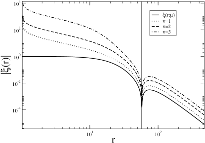
Figure 1: Absolute value of the reduced correlation function of the toy model described by Eq.3 (solid line) and of the ones corresponding to different values of the threshold parameter $\nu$ calculated by applying Eq.1. The amplification is non-linear at small scales, where $\xi(r;\mu>\tilde{\mu})>1$, linear at large scales, and the zero-crossing scale is invariant under biasing.

The correlation function given by Eq.3 is different from the one of a more realistic CDM model in the behavior at scales for $r<r_{zp}$: In the CDM model in that range of scales $\xi(r;\mu)$ has an approximate power-law behavior of the type $\xi(r;\mu)\sim r^{-1.5}$ with the introduction of some other characteristic scales. However the zero-crossing scale $r_{zp}$ is still a clear intrinsic feature which is not changed by the biasing scheme discussed in the previous section. At large scales $r>r_{zp}$ the CDM reduced correlation function has the same $-r^{-4}$ behavior as Eq.3. Both satisfy the important constraint

$$\int_{0}^{\infty}\xi(r;\mu)r^{2}dr=0$$ (5)

which has been called “the super-homogeneous condition”, in order to make clear the fact that this corresponds to a global condition on the correlation properties of particular systems which display a sort of long-range order, or, alternatively, they are more ordered than purely uncorrelated stochastic processes (e.g. Poisson) (Gabrielli, Joyce & Sylos Labini (2002)).

4 Sampling points in cosmological N-body simulations

Gravitational clustering in the regime of strong fluctuations is usually studied through gravitational N-body simulations. The particles are not meant to describe galaxies but collision-less dark-matter mass tracers (but see discussion in e.g. Baertschiger & Sylos Labini (2004)). During gravitational evolution complex non-linear dynamics make non-linear structures at small scales, while at large scales it occurs a linear amplification according to linear perturbation theory. Thus, while on large scales correlation properties do not change from the beginning — a part a simple linear scaling of amplitudes — at small scales non-linear correlations are built. Typically in these simulations non-linear clustering is formed up to scales of order of few Mpc (see e.g. Baertschiger, Joyce & Sylos Labini (2002)) and the intrinsic scale $r_{zp}$ is unchanged, as typically $r_{zp}>50$ Mpc/h in CDM models (see e.g. Gabrielli, Joyce & Sylos Labini (2002)).

At late times one can identify subsamples of points which trace the high density regions, and these would represent the “galaxies” whose statistical properties are ultimately compared with the ones found in galaxy samples. Here I consider the GIF galaxy catalog (Kauffmann et al. (1999)) constructed from a $\Lambda$CDM simulation run by the Virgo consortium (Jenkins et al. (1998)). The way in which this is done is to firstly identify the halos, which represent almost spherical structures with a power-law density profile from their center. The number of galaxies belonging to each halo is set proportional to the total number of points belonging to the halo to a certain power. This procedure identifies points lying in high density regions of the dark-matter particles. One may assign to each point a luminosity and a color on the basis of a certain criterion which is not relevant for what follows (see Sheth et al. (2001) and reference therein). The resulting catalog is divided into two subsamples based on “galaxy” color as in Sheth et al. (2001): (brighter) red galaxies (for which B-I is redder than 1.8) and (fainter) blue galaxies (B-I bluer than 1.8).

In summary four samples of points may be considered: (i) the original dark matter particles with N=$256^{3}$ particles (ii) all galaxies with N=15445 (iii) blue galaxies with N=11023 and (iv) red galaxies with N=4422. In Fig.2 the behavior of $\xi(r)$ for the different objects is shown .

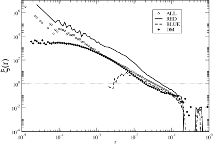
Figure 2: Reduced correlation function for the four samples of points selected in the simulation: the original dark matter (DM) field, all “galaxies” (ALL), blue galaxies (BLUE) and red galaxies (RED). Distances are given in units of the sample size L=141.3 Mpc/h.

One may notice that $\xi(r)$ for red (blue) galaxies has a larger (smaller) amplitude than the one of the original sample (all galaxies). The underlying dark matter particles show almost the same amplitude as all galaxies, although a change of slope at small scales is manifest. The amplification is linear, i.e. $\xi(r)$ for red galaxies shows almost the same functional behavior of that of all galaxies but with a larger amplitude. Clearly the original point distribution is not Gaussian, at least in the relevant range of scales considered, but characterized by strong fluctuations and thus one should explain such a mechanism of amplification (or de-amplification) differently from what has been proposed by Kaiser (1984). On the other hand the scale where the power-law behavior breaks down, and thus the scale $\xi(r_{zp})=0$, is invariant under sampling as for the simple Gaussian threshold biasing scheme discussed above: the amplitude independent characteristic scale is not changed under biasing. The biasing mechanism described above does not introduce new length scales in the system or change the intrinsic one, but it does alter the amplitude of the average density and thus any scale dependent on it (e.g. the scale such that $\xi(r_{0})=1$).

Note that the zero-crossing scale of $\xi(r)$ cannot be in general well established because of statistical fluctuations which affect any finite sample estimation of correlations. In this case however a clear signature of the zero-crossing scale is given by the sharp cut-off of the reduced correlation function, in a log-log plot, at the scale of order $r_{zp}$. This happens when the amplitude of the estimated $\xi(r)$ is about $10^{-2}$, so that statistical noise does not affect the measurement in a substantial way. In the case considered, in fact, the regime changes from being positively correlated, and larger than unity, to small anti-correlation. This is the way used hereafter to define the scale $r_{zp}$. In the general case, where the functional behavior of the correlation function is more complicated (e.g. with a very slow approach to zero) the way the zero-crossing scale is estimated must be clearly explored.

In order to test the reality of the zero-crossing scale, one may cut the sample at the scale $R_{s}\approx 0.3$ (in units normalized to the box side) and recompute the correlation function. No sensible change is found in the scale $r_{zp}$. As discussed below, this happens because the conditional density for scales $r>0.3$ is very well approximated by a flat behavior corresponding to the transition from strong to weak clustering, and the scale $r_{zp}$ is related, in this case, to the scale where the conditional density flattens.

Note that in the regime where $\xi(r)\gg 1$ no clear a priori prediction can be formulated on the amount of increase of amplitude of $\xi(r)$ with sampling. Actually the perspective on this problem is to choose a selection procedure such that it gives results similar to what is found in galaxy catalogs. Thus the observations are used to tune the selection in the simulations. The idea is in fact that one may change the way points are selected up to when a satisfactory agreement with what is observed in galaxy catalogs has been found. This can be true for the strongly correlated regime, but the selection employed does not change $r_{zp}$ which thus becomes the main length scale to be studied when relating observed galaxy distributions to simulations and ultimately to the distribution of the underlying dark matter particles.

In order to understand the origin of the amplification observed in the sampled point distributions it is useful to study the behavior of the conditional density which has a straightforward interpretation in terms of correlations (see Fig.3). This statistical tool gives the average number of points observed in an infinitesimal shell as a function of distance from a point of the distribution (and thus this is a conditional quantity) and can be written as (e.g. Gabrielli et al. 2004)

$${\langle n(r)\rangle_{p}}\equiv\frac{\langle n(\@vec{r})n(0)\rangle}{\langle n(0)\rangle}\;,$$ (6)

where $n(\@vec{r})$ is the microscopic particle number density. This is related to $\xi(r)$ by the equation

$$\xi(r)\equiv\frac{{\langle n(r)\rangle_{p}}}{n_{0}}-1\;.$$ (7)

being $n_{0}>0$ the ensemble average density of the distribution.

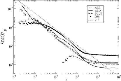
Figure 3: Conditional density for the samples of points shown in Fig.2. The conditional density for dark matter particles (DM) has been normalized arbitrarily. The reference line has a slope $\gamma=1.7$

The red galaxies are responsible for the strong correlations observed in the full sample as the conditional density is almost the same as for all galaxies at small scales. At large scales there is instead a fast decrease as the sample average of red galaxies is smaller than the one of all galaxies (there are less objects). The amplification of $\xi(r)$ of the red galaxies with respect to the full sample can be explained as an almost constant value of the conditional density at small scales together with a decrease of the sample density. It follows from Eq.7 that the amplitude of $\xi(r)$ is amplified if ${\langle n(r)\rangle_{p}}$ remains the same and $n_{0}$ is lowered. This means that for red galaxies the sampling is local, i.e. their conditional density is (almost) invariant at small scales. Clearly, as there are globally less objects, the sample density of red galaxies is smaller than that of all galaxies. On the other hand blue galaxies present only some residual correlations a small scales, and they are more numerous than red galaxies.

The main conclusion is that the intrinsic characteristic length of the model given by $r_{zp}$ (measured as discussed above) is not changed by this selection procedure, in close analogy with what happens in the simple Gaussian thresholding biasing scheme of a CDM field discussed in the previous section.

5 Finite size effects and the integral constraint

Concerning the study of the zero-crossing scale of $\xi(r)$ a point must be clarified in relation to the estimator of this statistical quantity. Suppose that one chooses the so-called full-shell estimator (Gabrielli et al. (2004)) defined as

$$\xi_{E}(r)=\frac{{\langle n(r)\rangle_{p}}^{E}}{n_{E}}-1$$ (8)

where $n_{E}$ is the density in a sphere of radius $R_{s}$ up to which ${\langle n(r)\rangle_{p}}^{E}$ can be estimated. As the sample density is estimated by

$$n_{E}=\frac{3}{4\pi R_{s}^{3}}\int_{0}^{R_{s}}{\langle n(r)\rangle_{p}}d^{3}r$$ (9)

it follows that

$$\int_{0}^{R_{s}}\xi_{E}(r)r^{2}dr=0\;.$$ (10)

This condition holds independently on $R_{s}$ and the true $\xi(r)$: Thus in a finite sample one finds the zero crossing of $\xi_{E}(r)$ no matter which are the true correlation properties of the distribution. For example $\xi(r)$ can be a simple positive power-law extending to scales much larger than $R_{s}$: its estimator in a finite sample will obey to Eq.10. The point to study is whether the zero-crossing scale depends, or not, on the sample volume.

In the case of a CDM-like correlation function, where a similar constraint holds in the whole space (see Eq.5) one can distinguish between the following behaviors (for simplicity, we neglect in the following discussion the effect of statistical noise in the estimator): (i) $R_{s}<r_{zp}$ — in this case the positively correlated range of scales at small scales will not be detected entirely, but an artificial zero-point will be introduced at scales comparable to $R_{s}$. In addition the amplitude of the estimator $\xi_{E}(r)$ is scale dependent. (ii) $R_{s}>r_{zp}$ — in this case the zero crossing scale will be well-defined, in the sense that changing $R_{s}$ the distance scale $r_{zp}$ will not change. Hoverer the negative correlated range of scales (i.e. $r>r_{zp}$) will be distorted (and the absolute value of $\xi_{E}(r)$ is increased) by the condition Eq.10 (see Fig.4).

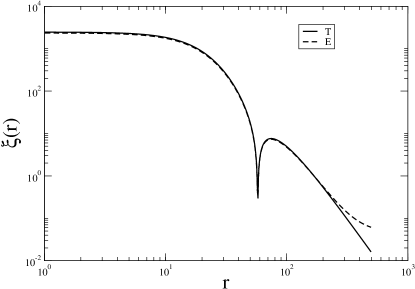
Figure 4: Estimation (E), through the full-shell estimator Eq.8, of the theoretical (absolute value) $\xi(r)$ (T) given by Eq.3: In this case $R_{s}=500>r_{zp}=60$. One may note that the negative tail is distorted in a non-linear way in order to satisfy Eq.10.

A similar situation happens when ${\langle n(r)\rangle_{p}}$ has a power-law behavior inside a given sample of size $R_{s}$. (Note that the following argument can be simply modified to any other functional behavior of ${\langle n(r)\rangle_{p}}$ in the regime where ${\langle n(r)\rangle_{p}}>n_{0}$). Suppose then that the scale where ${\langle n(r)\rangle_{p}}\approx n_{0}$ is larger than $R_{s}$ and that

$${\langle n(r)\rangle_{p}}=Br^{-\gamma}$$ (11)

where $3>\gamma>0$. Neglecting fluctuations, the estimation of the sample density from Eq.9 becomes

$$n_{E}=\frac{3B}{3-\gamma}R_{s}^{-\gamma}$$ (12)

so that the estimation of $\xi(r)$ can be written as (again, neglecting fluctuations)

$$\xi_{E}(r)=\frac{3-\gamma}{3}\left(\frac{r}{R_{s}}\right)^{-\gamma}-1\;.$$ (13)

In this case both the scales at which $\xi(r)=1,0$ are linearly dependent on the sample size $R_{s}$.

Note that the estimation in Eq.12 has been done by assuming that one can perform a volume average also at the scale of the sample: this means that one has made an average over different samples of size $R_{s}$. In case this is not possible (i.e. the usual situation in galaxy catalogs) significant deviation from the estimation given by Eqs.12-13 can be found (see Gabrielli et al. (2004) for a detailed explanation of this point).

It is worth noticing that while statistical noise may change the scale where $\xi(r_{zp})=0$, it does not change the fact that such a scale depends on the sample size as long as the conditional density has not become constant as a function of scale. However one should note that for a functional behavior of the type strong power-law correlations followed by a regime where $\xi(r)$ is very small (or zero or negative as in the CDM case) the scale $r_{zp}$ can be easily identified by the scale where a sharp break down from a power law behavior is manifest, which corresponds to the scale where ${\langle n(r)\rangle_{p}}\approx n_{0}$. This is actually the way in which the constraint imposed by Eq.10 is evident. The situation where the scale $r_{zp}$ corresponds to a real feature, i.e. $R_{s}\gg r_{zp}$, is much more problematic to be measured and it requires a very careful analysis of the estimator errors. For example the detection of very small amplitude correlations can be masked, at least, by Poisson noise going as $1/\sqrt{N}$.

6 Comparison with observations

The characterization of galaxy clustering is usually performed through the study of the reduced two-point correlation function. The result found in various galaxy catalogs is that $\xi_{E}(r)\approx A\times r^{-\gamma}$ when $\xi_{E}(r)\mathrel{\hbox to0.0pt{\lower 3.0pt\hbox{$\mathchar 536\relax$}\hss}\raise 2.0pt\hbox{$\mathchar 318\relax$}}1$ with $\gamma=1.7$ and $A$ is a constant which takes different values in different volume limited (hereafter VL) subsamples (e.g. Davis & Peebles (1983); Davis et al. (1988); Norberg et al. (2002); Zehavi et al. 2004A ).

One should note that a VL is constructed in such a way to contain all galaxies brighter than a certain absolute magnitude threshold and it is limited by a distance depending on the apparent magnitude limit of the galaxy catalog and on the absolute magnitude threshold considered (e.g., Davis & Peebles (1983)). This implies that a VL sample is identified (at least) by two cuts, one in the distance $R_{VL}$ and one in the corresponding absolute magnitude $M_{VL}$, the relation between the two being (at small redshift, neglecting corrections)

$$M_{VL}=m_{lim}-5\log_{10}R_{VL}-25$$ (14)

where $m_{lim}$ is the apparent magnitude limit of the considered galaxy survey and $R_{VL}$ is measured in Mpc/h. Thus, when one increases $R_{VL}$ only galaxies with brighter absolute luminosity (decreasing absolute magnitude $M<M_{VL}$) are included in the sample. (In latest surveys like SDSS and 2dF, there are two cuts in apparent magnitude, and thus a VL is identified by two cuts in absolute magnitude and two in distance: this complicates the estimation of the depth of the samples but does not introduce a substantial change in the following discussion).

Given the two parameters $R_{VL}\,,M_{VL}$ defining a VL sample, one may consider (at least) two different effects which may cause the amplification of $\xi_{E}(r)$: (i) a luminosity (or sampling) effect related to the selection of different class of objects in different VL samples; (ii) a finite-size effect related to the change of the volume of the samples considered when the absolute magnitude cut is changed. In other words the variation of the amplitude of $\xi_{E}(r)$ can be related to a sampling effect (e.g. to Eq.1) or to a volume effect (e.g. to Eq.13): The situation is illustrated in Figs.5-6.

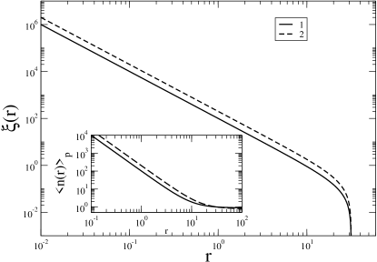
Figure 5: Amplification of $\xi_{E}(r)$ due to a sampling procedure similar to what is found in N-body simulation. The underlying particle distribution (1) and the selected ones (2) have a different amplitude in the regime of strong clustering but show the same zero-point crossing scale in the reduced correlation function which has a power-law decay up to a definite scale. In the insert panel it is shown the corresponding behavior of the conditional density. Note that the scale $r_{zp}$ coincides with the scale where ${\langle n(r)\rangle_{p}}\approx$ constant.

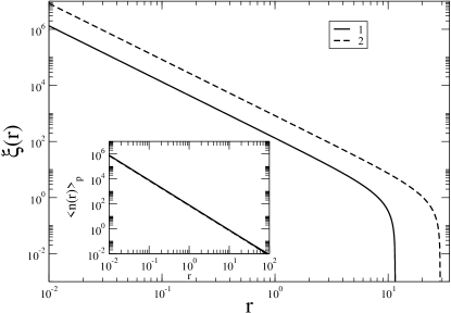
Figure 6: In the case the distribution has a conditional density with a power-law behavior up to the sample size (1), then the amplitude of $\xi_{E}(r)$ and its zero-crossing scale depends linearly on the sample size (2) if the sample size is larger than the scale where ${\langle n(r)\rangle_{p}}$ has a clear flattening toward a constant value. In the insert panel it is shown the corresponding behavior of the conditional density: in this case the two lines coincide, the case (2) extending to larger scales.

Note that the variation of the amplitude of $\xi_{E}(r)$ (or of its Fourier conjugate the power spectrum) is usually (e.g. Davis & Peebles (1983); Davis et al. (1988); Norberg et al. (2002); Zehavi et al. 2004A ) ascribed to the fact that galaxies of different luminosity are differently clustered in the sense that brighter galaxies have a larger amplitude than fainter ones (this is usually called “luminosity bias”): i.e. $A=A(M_{VL})$ is an increasing function of the absolute luminosity $M_{VL}$ of the considered galaxies (e.g. Norberg et al. (2002); Zehavi et al. 2004A ). Also for galaxy clusters a similar variation in the amplitude, although larger, has been found (e.g. Bahcall & Soneira (1983)) where the variation is ascribed to the richness of the clusters considered. In brief this variation is ascribed to some specific ways of sampling the (galaxy or cluster) point distribution. If this would be the case than one should find, for the zero-crossing length scale $r_{zp}$ a situation analogous to the one shown in Fig.5: i.e. this scale should be the same for different objects.

Thus in order to distinguish between the two different mechanics of amplification of $\xi(r)$ one has an indirect and a direct test. The former consists in the study of the stability of the zero-crossing length scale in different samples, while the latter is represented by the determination of the conditional density in VL samples. As the conditional density is not usually estimated (e.g. Zehavi et al. 2004B, Norberg et al., 2002) I need to consider also the stability of $r_{zp}$. Below I will comment about the relation with the measurements of ${\langle n(r)\rangle_{p}}$ recently performed by Hogg et al. (2005) and the various determinations summarized in Gabrielli et al. (2004).

It is interesting to briefly review some determinations in redshift space of the scale $r_{zp}$: in the CfA1 sample $r_{zp}\approx 20$ Mpc/h (Davis & Peebles (1983)); Park et al. (1994) found, in the CfA2 catalog, a larger value of about $r_{zp}\approx 30$ Mpc/h (see their Fig.10) and Benoist et al. (1996) found that $r_{zp}$ is not stable in different VL samples of the SSRS2 survey, changing from 10 to about 50 Mpc/h (see their Fig.1). More recently it has been found that $r_{zp}\approx 40$ Mpc/h in the Two degree Field Galaxy Redshift Survey (Hawkins et al. 2003 ). The latest determination has been performed by Eisenstein et al. (2005) by considering the Luminous Red Galaxies sample from the SDSS. This sample covers the largest volume of universe up to now. In Eisenstein et al. (2005) the zero-point of the correlation is found to be at a scale of about 120 Mpc/h (see their Figs.2-3). Thus it seems that, up to now, in galaxy samples, the length scale $r_{zp}$ is related to the length scale $r_{0}$ (defined as $\xi(r_{0})=1$): they are both sample size dependent. Whether the latest measurement by Eisenstein et al. (2005) is stable will have to be shown by the analysis in larger samples.

Note that, as discussed above, one of the main characteristic of the selection mechanisms usually considered is that the zero-crossing scale of $\xi(r)$ is invariant under sampling. Thus even if one uses a very particular kind of objects, results on the zero-crossing scale have to be the same for any other kind of objects if the difference in the correlation function (or power spectrum) are explained by a selection effect similar to what is found in the N-Body simulations. If the zero-crossing scale is instead not found to be stable in different samples and thus for different objects, this is a clear indication that correlation properties are finite-size dependent in the sense of Fig.6.

The direct test (corresponding to the insert panels in Figs.5-6) for this has been implicitly performed by Hogg et al. (2005) where they measured the (integrated) conditional density for the same Luminous Red Galaxies sample considered by Eisenstein et al (2005). They in fact find that the conditional density, having a power law behavior with exponent $\gamma\approx 1$ up to $20\div 30$ Mpc/h, shows a slow crossover toward homogeneity, reaching a constant value at about 70 Mpc/h. These results support the conclusions drawn here, that the zero-point crossing scales found in previous and smaller volume surveys is a finite size effect. The results by Hogg et al. (2005) are then in agreement with those of Eisenstein et al. (2005): here we note that the flattening of ${\langle n(r)\rangle_{p}}$ occurs at scales comparable to the sample size and thus this situation requires a careful study of larger samples to confirm these results over a substantial range of scales (see discussion in Joyce et al. 2005).

7 Conclusions

The study of the dependence of the zero-crossing scale as a function of the size of a given sample is already a vailable test to distinguish between the different effects producing the variation of the amplitude of $\xi(r)$. As long as it is found to be dependent on the finite sample size, this means that all amplitudes related to $\xi(r)$ are also finite size dependent. In such a situation a more clear way to study the problem is represented by the analysis of the conditional density ${\langle n(r)\rangle_{p}}$ (see e.g. Gabrielli et al. (2004)). From a review of the literature it seems that the scale $r_{zp}$ has grown from 20 Mpc/h in the CfA1 sample (Davis & Peebles (1983)) to about 120 Mpc/h in the latest SDSS data (Eisenstein et al. (2005)). Analogously the scale $r_{0}$ (defined as $\xi(r_{0})=1$) has grown from about 5 Mpc/h in the CfA1 (Davis & Peebles (1983)) to about 13 Mpc/h in the SDSS sample (Zehavi et al. 2004B ).

This implies that the explanation of the amplitude variation of $\xi(r)$ by luminosity bias (brighter objects have larger amplitudes) is untenable. Such a variation can be instead explained as a finite size effect. To directly test this fact one may simply measure the conditional density and results for this quantity (Sylos Labini et al. 1998, Hogg et al., 2005) unambiguously support the fact the the amplitude variation of $\xi(r)$, or of its zero-crossing length, are finite-size effects (see Figs.5-6). This situation implies that $r_{0}$ is sample size dependent up to the scale where ${\langle n(r)\rangle_{p}}$ has a clear crossover. If one considers such a scale to be 70 Mpc/h, as suggested by Hogg et al. (2005), then $r_{0}\approx 13$ Mpc/h for galaxies of any luminosity. Note that the prediction of Eq.13 does not apply in this situation as the conditional density measured by Hogg et al. (2005) shows two different behaviors in the strongly clustering regime: a simple power-law up to about $20$Mpc/h a a slow crossover up to 70 Mpc/h. In this situation the estimation of $r_{0}$ has to be done numerically.

The difference between the zero-crossing length scales, found by the sharp cut-off in a log-log plot of the correlation function, in the galaxy catalogs extracted from N-body simulations (which is about 30 Mpc/h) and the one detected by (Eisenstein et al. (2005)) for the largest observational sample of the SDSS available up to now, is of about a factor five. In the situation considered here the zero-point of $\xi(r)$ is the scale where ${\langle n(r)\rangle_{p}}\approx n_{0}$ and thus this is related to the size of the largest non-linear structure in the distribution. This implies that structures formed in N-body simulations are smaller than galaxy structures. This can be directly tested by comparing the scale where ${\langle n(r)\rangle_{p}}\approx$ const. in simulations and in galaxy samples (see discussion in Joyce et al., 2005).

It is important to stress that the conditional density in N-body simulations (see Fig.3) has a slope of about $\gamma=-1.7$ while in galaxy catalogs Sylos Labini et al. (1998) and Hogg et al. (2005) have measured $\gamma=1$. While the analysis of $\xi(r)$ does not give a clear determination of the slope $\gamma$, as it is affected by a finite size effect when ${\langle n(r)\rangle_{p}}$ is a power-law, the analysis of the conditional density provides with a clear result (see discussion in Gabrielli et al. 2005). In other words, while the comparison of $\xi(r)$ in simulations and galaxy samples can be misleading, this is not the case for ${\langle n(r)\rangle_{p}}$.

One should also note that in N-body simulations the slope is determined in real space, while in results in galaxy catalogs considered here are in redshift space. However the scales involved (some tens Mpc/h where peculiar velocities are expected to be small) and the large difference in the slopes found (about 0.7) point toward a real difference between structures formed in N-body simulations and observed in galaxy catalogs.

It is worth noticing that the scale $r_{zp}$, in CDM models, is simply related to the so-called turn-over wave-number of the power spectrum, i.e. where the power spectrum changes regime from negative to positive power law. In this respect, I note that for the determination of the power-spectrum of density fluctuations a finite size effect in the amplitude and in the location of the turn-over scale, in a similar way to what happens for $\xi(r)$, is expected to be present as long as the distribution has strong clustering inside a given sample (Sylos Labini & Amendola (1996)). Such a situation allows one to simply relate the results of Tegmark et al. (2004) for the power spectrum in the SDSS survey, to the results obtained by the real space correlation function analysis by Zehavi et al. (2004B).