Nonlinear Evolution of the Magnetothermal Instability in Two Dimensions

Abstract

In weakly magnetized, dilute plasmas in which thermal conduction along magnetic field lines is important, the usual convective stability criterion is modified. Instead of depending on entropy gradients, instability occurs for small wavenumbers when $(\partial P/\partial z)(\partial\ln T/\partial z)>0$, which we refer to as the Balbus criterion. We refer to the convective instability that results in this regime as the magnetothermal instability (MTI). We use numerical MHD simulations which include anisotropic electron heat conduction to follow the growth and saturation of the MTI in two-dimensional, plane parallel atmospheres that are unstable according to the Balbus criterion. The linear growth rates measured in the simulations agree with the weak field dispersion relation. We investigate the effect of strong fields and isotropic conduction on the linear properties and nonlinear regime of the MTI. In the nonlinear regime, the instability saturates and convection decays away, when the atmosphere becomes isothermal. Sustained convective turbulence can be driven if there is a fixed temperature difference between the top and bottom edges of the simulation domain, and if isotropic conduction is used to create convectively stable layers that prevent the formation of unresolved, thermal boundary layers. The largest component of the time-averaged heat flux is due to advective motions. These results have implications for a variety of astrophysical systems, such as the temperature profile of hot gas in galaxy clusters, and the structure of radiatively inefficient accretion flows.

1 Introduction

In dilute astrophysical plasmas, the mean free path between particle collisions can be much larger than the ion gyroradius. In this circumstance, the equations of magnetohydrodynamics (MHD) which describe the dynamics of the plasma must include anisotropic transport terms for energy and momentum due to near free-streaming motions of particles along magnetic field lines (Braginskii, 1965). The parallel thermal conductivity of the electrons is larger than that of the ions by a factor proportional to $(m_{i}/m_{e})^{1/2}$, whereas the parallel viscosity of the ions is larger than that of the electrons by the same factor. Thus, provided that collisions are still frequent enough to keep the distributions of the velocity components parallel and perpendicular to the magnetic field in equilibrium, the usual equations of MHD must be supplemented with an anistropic electron heat conduction term, and an anisotropic ion viscosity. Moreover, since the ratio of ion viscosity to electron heat conduction is proportional to $(m_{e}/m_{i})^{1/2}$, it is often sufficient to neglect the former, and consider only the effect of anisotropic electron heat conduction. In a rotating system, even a small ion viscosity may be important (Balbus, 2004). If the parallel and perpendicular temperature of particles are not in equilibrium, more complex closures are required (Hammett & Perkins, 1990).

The implications of anisotropic transport terms on the overall dynamics of dilute astrophysical plasmas is only beginning to be explored (Balbus, 2001; Quataert, Hammett, & Dorland, 2002; Sharma, Hammett, & Quataert, 2003). One of the most remarkable results obtained thus far is that the convective stability criterion for a weakly magnetized dilute plasma in which anisotropic electron heat conduction occurs is drastically modified from the usual Schwarzschild criteria (Balbus, 2000). In particular, stratified atmospheres are unstable if they contain a temperature (as opposed to entropy) profile which is decreasing upward. There are intriguing analogies between the stability properties of rotationally supported flows (where a weak magnetic field changes the stability criterion from a gradient of specific entropy to a gradient of angular velocity), and the convective stability of stratified atmospheres (where a weak magnetic field changes the stability criterion from a gradient of entropy to a gradient of temperature). The former is a result of the magnetorotational instability (MRI; Balbus & Hawley, 1998). The latter is a result of anisotropic heat conduction. To emphasize the analogy, we will refer to this new form of convective instability as the magnetothermal instability (MTI). The MTI may have profound implications for the strucuture and dynamics of many astrophysical systems.

In this paper, we use numerical methods to explore the nonlinear evolution and saturation of the MTI in two-dimensions. We adopt an arbitrary vertical profile for a stratified atmosphere in which the entropy increases upward (and therefore is stable according to the Schwarzschild criterion), but in which the temperature is decreasing upwards (and therefore is unstable according to the Balbus criterion, $(\partial P/\partial z)(\partial\ln T/\partial z)>0$). We confirm the linear growth rates predicted by Balbus (2000) for dynamically weak magnetic fields, and numerically measure the growth rates for stronger fields. We follow the evolution of the instability into the nonlinear regime, and show that it results in vigorous convective turbulence and heat transport. These results may have implications for radially stratified atmospheres in which anisotropic transport may be present, including x-ray emitting gas in clusters of galaxies (Fabian, 1994; Zakamska & Narayan, 2003), atmospheres of strongly magnetized neutron stars, and radiatively inefficient accretion flows (Stone, Pringle, & Begelman, 1999; Narayan, Mahadevan, & Quataert, 1998).

This paper is organized as follows. In §2, we describe our numerical methods and initial conditions. In §3, we compare the computational results to the analytical results of linear theory. In §4 and §5 we present the results from the non-linear regime and saturated states for two different choices of boundary conditions for the temperature at the top and bottom of the computational domain. Finally, in §6 we summarize our results, discuss applications, and describe future work.

2 Method

2.1 Equations of MHD with Anisotropic Heat Conduction

The equations of MHD with the addition of the heat flux, $\mathbf{Q}$, and a vertical gravitational acceleration, ${\bf g}=-g_{0}{\bf\hat{z}}$ are

$$\frac{\partial\rho}{\partial t}+\mathbf{\nabla}\cdot\left(\rho\mathrm{\mathbf{v}}\right)=0,$$ (1)

$$\frac{\partial(\rho\mathbf{v})}{\partial t}+\mathbf{\nabla}\cdot\left[\rho\mathbf{vv}+\left(p+\frac{B^{2}}{8\pi}\right)\mathbf{I}-\frac{\mathbf{BB}}{4\pi}\right]+\rho\mathbf{g}=0,$$ (2)

$$\frac{\partial\mathbf{B}}{\partial t}+\mathbf{\nabla}\times\left(\mathbf{v}\times\mathbf{B}\right)=0,$$ (3)

$$\frac{\partial E}{\partial t}+\mathbf{\nabla}\cdot\left[\mathbf{v}\left(E+p+\frac{B^{2}}{8\pi}\right)-\frac{\mathbf{B}\left(\mathbf{B}\cdot\mathbf{v}\right)}{4\pi}\right]+\mathbf{\nabla}\cdot\mathbf{Q}+\rho\mathbf{g}\cdot\mathbf{v}=0,$$ (4)

where the symbols have their usual meaning. The total energy $E$ is given as

$$E=\epsilon+\rho\frac{\mathbf{v}\cdot\mathbf{v}}{2}+\frac{\mathbf{B}\cdot\mathbf{B}}{8\pi},$$ (5)

with the internal energy, $\epsilon=p/(\gamma-1)$. For this paper, we assume $\gamma=5/3$ throughout.

The heat flux contains contributions both from electron motions (which are constrained to move primarily along field lines) and from isotropic transport which may arise due to photons or particle collisions which drive cross field diffusion. Thus, ${\bf Q}={\bf Q}_{C}+{\bf Q}_{R}$, where

$$\mathbf{Q}_{C}=-\chi_{C}\mathbf{\hat{b}\hat{b}}\cdot\mathbf{\nabla}T,$$ (6)

$$\mathbf{Q}_{R}=-\chi_{R}\mathbf{\nabla}T,$$ (7)

where $\chi_{C}$ is the Spitzer Coulombic conductivity (Spitzer, 1962), $\mathbf{\hat{b}}$ is a unit vector in the direction of the magnetic field, and $\chi_{R}$ is the coefficient of isotropic conductivity, ostensibly due to radiation. We consider both $\chi_{C}$ and $\chi_{R}$ as free parameters in the problem and will vary both independently.

2.2 Initial Equilibrium Conditions

We now specify a vertical equilibrium state in which we can study the linear modes and nonlinear evolution of the MTI. The first step is to choose an Ansatz for the form of the gravitational field. In this paper, we adopt the simplest choice of a constant vertical acceleration: $g(z)=-g_{0}$. This form is appropriate for a thin plane-parallel atmosphere. Alternative choices in which the gravitational acceleration varies with height would be appropriate for the vertical structure of a thin accretion disk, or the radial structure of a self-gravitating gas sphere. However, since the MTI is a local instability, the evolution of modes with wavelengths much smaller than the scale height, $H\sim c_{s}^{2}/g$, where $c_{s}^{2}$ is the adiabatic sound speed, should be independent of the form of $g(z)$. We will consider other profiles in applications specific to particular astrophysical systems in future work.

We next make the Ansatz that the temperature in the atmosphere decreases with height, while the entropy increases with height. Perhaps the simplest vertical equilibrium state which satisfies this condition is a power law:

$$T(z)=T_{0}(1-z/z_{0}),$$ (8)

$$\rho(z)=\rho_{0}(1-z/z_{0})^{2},$$ (9)

$$p(z)=p_{0}(1-z/z_{0})^{3},$$ (10)

where $z_{0}$ is a constant. We have assumed that the magnetic pressure is small compared to the gas pressure ($\beta=8\pi p/B^{2}\gg 1$), so that the vertical structure is given by the solution of the equation of hydrostatic equilibrium. Of course, any power-law profile with $T$ decreasing with height would do; however, by choosing a linear profile we guarantee that the vertical gradients are shallow and easier to resolve numerically. To satisfy hydrodynamic stability, we choose $T_{0}=\rho_{0}=p_{0}=g_{0}=1$ in an appropriate system of units. Convective stability places a constraint on the entropy gradient via the Schwarzschild criterion, namely, $dS/dz>0$. For our choice of initial conditions convective stability to perturbations requires, $0<z_{0}^{-1}<2/5g_{0}$. Setting $z_{0}=3$ satisfies the hydrodynamic equilibrium and convective stability constraints. These constants determine the adiabatic sound speed in the domain to be

$$c_{s}^{2}(z)=\frac{\gamma p(z)}{\rho(z)}=\frac{5}{3}\left(1-\frac{z}{3}\right).$$ (11)

By using a simulation domain which is small compared to the scale height, $H=C_{s}^{2}/g\approx 1.67$, we ensure the sound speed does not vary much from the top to the bottom of the box.

Finally, we add a weak horizontal magnetic field so that the domain contains either a zero or net magnetic flux:

$$B_{x}(z)=\left\{\begin{array}[]{ll}B_{0}&\textrm{net flux}\\ B_{0}\sin\left(\frac{2\pi z}{L_{z}}\right)&\textrm{zero flux;}\end{array}\right.$$ (12)

The Alfvén speed becomes

$$v_{A}^{2}(z)=\frac{B_{x}^{2}(z)}{4\pi\rho(z)}=\frac{B_{0}^{2}}{4\pi}\left(1-\frac{z}{3}\right)^{-2}.$$ (13)

for the case of a uniform horizontal field. The value of $B_{0}$ is chosen to be small so that tension effects are unimportant in the linear regime, that is typically $v_{A}\ll c_{s}$. We also investigate the effects of strong fields in suppressing the instability.

2.3 Linear Stability Properties of the MTI

If $\chi_{R}=0$, the heat flux in the initial state is zero because the magnetic field lines are parallel to the isotherms, and it represents an equilibrium. Now imagine a small vertical perturbation that partially aligns the magnetic field with the background temperature gradient, that is $\mathbf{B}\cdot\bf{\nabla}T\neq 0$. Heat is now able to flow from the hotter to the colder regions, causing them to become buoyant and rise. This, in turn, causes the magnetic field to become more aligned with the background temperature gradient; increasing the heat flow. Thus, a growing instability is generated.

A quantitative understanding of the instability is gained by considering the linearized equations of MHD (eq.[1-5]) with the specification of a heat flux that is purely Coulombic. The details can be found in (section 4, Balbus, 2000).

We introduce the Brunt-Väisälä frequency, $N$,

$$N^{2}=-\frac{1}{\gamma\rho}\frac{\partial P}{\partial z}\frac{\partial\ln S}{\partial z},$$ (14)

the frequency of vertical oscillations in a stably stratified atmosphere. Preserving Balbus’ notation, we also define two useful quantities,

$$\chi_{c}^{\prime}=\frac{\gamma-1}{P}\chi_{c}\qquad\textrm{and}\qquad\chi^{\prime}=\frac{\gamma-1}{P}\left(\chi_{c}+\chi_{R}\right).$$ (15)

Using the Fourier convention for perturbations, $\exp{(\sigma t+ikx)}$, and in the limit of a weak magnetic field, $k^{2}v_{A}^{2}\ll 1$, the dispersion relation simplifies to the non-dimensionalized form

$$\left(\frac{\sigma}{N}\right)^{3}+\frac{1}{\gamma}\left(\frac{\sigma}{N}\right)^{2}\left(\frac{\chi^{\prime}Tk^{2}}{N}\right)+\left(\frac{\sigma}{N}\right)+\frac{d\ln T}{d\ln S}\left(\frac{\chi^{\prime}_{c}Tk^{2}}{N}\right)=0,$$ (16)

Solutions to the dispersion relation are plotted in Figure 1. The lower branches are stable oscillations. Note that in Figure 5 of (Balbus 2000) the factor of $1/\gamma$ multiplying the second term of equation 16 is omitted. Our choice of initial conditions sets the constant $d\ln T/d\ln S=-3$. By analysis of the Routh-Hurwitz criterion (Section 4.3, Balbus, 2000), the instability criterion is

$$k^{2}v_{A}^{2}-\frac{\chi^{\prime}_{C}}{\rho\chi^{\prime}}\frac{\partial P}{\partial z}\frac{\partial\ln T}{\partial z}<0.$$ (17)

In the limit of infinitesimal wavenumber, the instability criterion simply requires the temperature and pressure gradients to be in the same direction, i.e.,

$$\frac{\partial P}{\partial z}\frac{\partial\ln T}{\partial z}>0.$$ (18)

We will refer to the instability criterion equation (18) as the Balbus criterion. The instability criterion of the magnetorotational instability (Balbus & Hawley, 1998) can be written

$$k^{2}v_{A}^{2}+\frac{d\Omega}{d\ln R}<0,$$ (19)

where $\Omega$ is the angular velocity. The similarity between the MRI and the MTI is self-evident. Strong magnetic fields will stabilize short wavelength perturbations in both instabilities through tension. This point will be addressed in §3.2 in more detail.

2.4 Numerical Algorithms for studying the Nonlinear Regime

We follow the MTI into the nonlinear regime using the Athena MHD code (Gardiner & Stone, 2005). Athena is an unsplit Godunov method for ideal MHD that utilizes constrained transport to preserve the divergence-free constraint of the magnetic field. Isotropic and anisotropic heat conduction are added to the basic MHD algorithm through operator splitting. By finite differencing the diffusion terms in local field line coordinates, we are able to keep the ratio of parallel to perpendicular thermal diffusion greater than at least $10^{3}$ for any orientation of the field with respect to the grid (and much larger than that when the field is closely aligned with grid). We show in section 3.3 that the level of isotropic conduction added by numerical truncation error has a negligible effect on the linear properties of the MTI. Details of the numerical methods used for anisotropic conduction, including tests, are given in the appendix.

All of the simulations presented in this paper are performed on a two dimensional grid, with horizontal and vertical coordinates $x$ and $z$. The size of the domain is $L_{x}=L_{z}=0.1$. Our standard numerical resolution is $100^{2}$ for single-mode studies and $128^{2}$ for multi-mode studies, although we have performed resolution studies which span grid resolutions from $64^{2}$ to $512^{2}$. By using a box size which is small compared to the scale height, we ensure the sound speed varies only slightly from the top to the bottom of the domain. From equation (11) the average sound speed is $\bar{c_{s}}\approx 1.28$, giving a sound crossing time, $\bar{\tau_{s}}\approx 7.81\times 10^{-2}$. For comparison, the typical magnetic field strength in the initial state is chosen to be $B_{0}/\sqrt{4\pi}=10^{-3}$, giving an Alfvén speed of $v_{A}=10^{-3}$, and an Alfvén crossing time of 100.

We use periodic boundary conditions in the horizontal $x$-coordinate. We study the saturation of the MTI using two different boundary conditions in the vertical $z$-coordinate. In both cases, reflecting boundary conditions are applied to all variables except the internal energy, in which an extrapolation is used so that the pressure gradient balances the gravitational acceleration at the boundary—an important consideration for Godunov schemes (see below). In addition, for the first case, the boundary temperature is set equal to the temperature in the last active computational cell in the grid; that is a Neumann boundary condition is used for the temperature. We will refer to this boundary condition for the temperature as “adiabatic boundaries,” as heat is not exchanged. For the second case, the boundary temperature is held fixed at constant values at the upper and lower boundaries; that is a Dirichlet boundary condition is used for the temperature. This latter case drives a heat flux into and out of the domain. We will refer to this boundary condition for the temperature as “conducting boundaries.”

By periodicity, there can be no net flux of mass, momentum, or energy in the horizontal direction. However, because we do not enforce $V_{z}=0$ on the vertical boundaries explicitly, it is possible through numerical truncation error to have a net flux of mass or momentum through the vertical boundaries. Note we specifically permit a net flux of energy (heat) through the vertical boundary. For Godunov schemes like Athena, in order for the flux difference due to the vertical pressure gradient to exactly balance the gravitational acceleration source term, the gravitational source terms must be incorporated directly into the computation of the fluxes. This requires substantial modification of the underlying MHD algorithm; thus, we utilize the much simpler procedure of extrapolating the pressure at the boundary to cancel the source terms. We have checked the accuracy of our method by keeping track of the the conservation of net magnetic flux and momentum in the simulation domain. The fractional error of these is no more than $10^{-12}$ and $10^{-6}$ respectively over thousands of dynamical times.

To seed the MTI, small amplitude perturbations are added to the vertical velocity. To seed a single mode, a perturbation of the form

$$v_{z}(x)=v_{0}\sin\left(\frac{n\pi x}{L_{x}}\right),$$ (20)

is used, where $n$ is the mode of the perturbation. Note single mode perturbations are not smoothed at the vertical boundaries. To seed multiple modes, Gaussian white noise velocity perturbations which are smoothed in the vertical direction using $\sin(\pi z/L_{z})$ are used. The standard perturbation amplitude is $v_{0}=10^{-4}$, which is much less than either the Alfvén or sound speed.

3 Comparison to Linear Theory

3.1 Weak Field Limit

As a test of our numerical algorithms, we have performed a series of simulations using a grid of $100^{2}$ and single mode perturbations where $\chi_{C}$ varies from $2.5\times 10^{-5}$ to $10^{-3}$ and $\chi_{R}=0$ with a perturbation wavelength equal to the horizontal domain size. The initial conditions contain a uniform horizontal field of uniform amplitude $B_{0}/\sqrt{4\pi}=10^{-3}$ (net flux) and an initial velocity perturbation of amplitude $v_{0}=2\times 10^{-4}$. Adiabatic boundary conditions are used on the vertical boundaries. We measure the linear growth rate in the simulation by extracting the horizontally-averaged amplitude of the velocity perturbation seeded in equation 20 at different times and applying the relationship,

$$\sigma=\frac{\ln(\bar{v}(t_{2})/\bar{v}(t_{1}))}{t_{2}-t_{1}}.$$ (21)

The measured growth rates are plotted as crosses on the dispersion relation for linear modes in the weak field limit shown in Figure 1.

The measured growth rates from the simulations are in excellent agreement with the predictions of linear theory. Given that the Brunt-Väisälä frequency and temperature vary vertically over the simulation domain, the initialized abscissa is actually a range, the midpoint of which is plotted. For example, one simulation has a range of $\left(\chi^{\prime}Tk^{2}/N\right)\in[1.019,1.072]$ which gives a theoretical growth rate of $\sigma_{\mathrm{theory}}\in[0.279,0.289]$. Analysis of the linear phase of the simulation gives a growth rate as $\sigma_{\mathrm{simulation}}\in[0.279,0.295]$, a relatively small error. Due to the difficulty of defining a systematic error convention for this case, error bars are not shown, and the average values are plotted. We conclude our numerical algorithms for anistropic conduction accurately capture the MTI.

3.2 Dependence on Magnetic Field Strength

Like the MRI, the magnetothermal instability can be stabilized at large $k$ by tension. Equation 17 shows the dependence of the MTI instability criterion on the magnetic field (implicitly through the Alfvén velocity). We define a stability parameter, $\eta$, as

$$\eta=\frac{k^{2}v_{A}^{2}}{\sigma^{2}_{\mathrm{max}}},$$ (22)

where the maximum growth rate, $\sigma_{\mathrm{max}}$, is given by

$$\sigma^{2}_{\mathrm{max}}=\frac{\chi^{\prime}_{C}}{\rho\chi^{\prime}}\frac{\partial P}{\partial z}\frac{\partial\ln T}{\partial z}.$$ (23)

Figure 2 shows the effect of varying the magnetic field on the growth rate holding all other parameters fixed. We vary $B_{0}/\sqrt{4\pi}$ from $10^{-4}$ to 0.03 while the conductivity is held fixed at $\chi_{C}=10^{-4}$ and $\chi_{R}=0$. All other parameters are the same as specified in the previous section. As the magnetic field (and stability parameter) approach zero, the growth rate asymptotes to its maximum value given by the weak field dispersion relation, equation 16. As the magnetic field increases in strength the growth rate decreases until $\eta=1$, at which point the instability is entirely quenched. The curve in Figure 2 is approximated roughly by the fit

$$\sigma(\eta)=\left\{\begin{array}[]{ll}(1-\eta)\sigma_{\mathrm{max}}&\eta\leq 1,\\ 0&\eta>1.\end{array}\right.$$ (24)

3.3 Effect of Isotropic Conduction

Isotropic conduction can damp the linear growth rates of the MTI, thus limiting its effect to regions where anisotropic conduction dominates. The anisotropy factor, $Q$, is defined as

$$Q\equiv\frac{\chi_{C}^{\prime}}{\chi^{\prime}}=\frac{\chi_{C}}{\chi_{C}+\chi_{R}},$$ (25)

Equation 16 can be easily rewritten in terms of $Q$ as

$$\left(\frac{\sigma}{N}\right)^{3}+\frac{1}{\gamma}\left(\frac{\sigma}{N}\right)^{2}\left(\frac{\chi^{\prime}Tk^{2}}{N}\right)+\left(\frac{\sigma}{N}\right)+\frac{d\ln T}{d\ln S}\left(\frac{\chi^{\prime}Tk^{2}}{N}\right)Q=0.$$ (26)

To study the effect of isotropic conduction, we hold the total value of the conductivity, $\chi_{\mathrm{tot}}=\chi_{C}+\chi_{R}$ fixed. Alternatively, this can be understood as choosing a fixed non-dimensionalized wavenumber in the dispersion relation. We then vary the anisotropy factor, $Q$. This linear study uses conducting boundary conditions at a resolution of $100^{2}$. Initial conditions are a magnetic field of $B_{0}/\sqrt{4\pi}=5\times 10^{-4}$ yielding a net magnetic flux and a single-mode perturbation. Figure 3 shows the effect of isotropic conductivity on the growth rate for a fixed $\chi_{\mathrm{tot}}=10^{-4}$. The solid line in this plot comes from the solution of equation 16.

As the conduction becomes purely anisotropic, the growth rate asymptotically approaches the weak-field value calculated previously. When isotropic conduction dominates, the instability is totally suppressed. The measured growth rates are slightly over-estimated compared to linear theory for $Q\sim 1$. If one examines the value $Q=0.01$, weak-field theory predicts a finite growth-rate; however, the simulation shows zero growth. In this case, the two terms of Equation 17 are of similar order and the weak-field treatment breaks down.

An important result to note is that a small amount of isotropic conduction, $Q=0.99$, does not change the growth rate significantly from no isotropic conduction, $Q=1.0$. This fact implies that the anisotropic conduction routine does not need to preserve anisotropy to as many orders of magnitude as is needed for tokamak plasma simulations. We show in the appendix that our algorithm results in a ratio of parallel to perpendicular conductivity of $>10^{3}$ for arbitrary orientations of the field with respect to the grid. Thus, even though the effective $Q$ in our simulations is not as close to one as in a real plasma, it is close enough, e.g. $Q_{\rm eff}>0.99$, that the resulting dynamics should be unaffected.

4 Non-Linear Regime of the Adiabatic Boundary Condition

Table 1 is a list of all runs using adiabatic boundary conditions discussed in this paper. N1-N2 are characteristic non-linear studies whose properties are displayed in this paper. Runs A1-A5 explore the effect of initial magnetic field strength on saturation. Of course, many more combinations of these parameters can and have been simulated. An illustrative subset is presented here.

4.1 Uniform Magnetic Field

As a fiducial model, we consider a single-mode perturbation with a purely anisotropic conductivity $\chi_{C}=10^{-4}$ and a uniform magnetic field strength $B_{0}/\sqrt{4\pi}$ of $5.0\times 10^{-4}$ labeled Run N1 in Table 1. Figure 4 shows plots of the magnetic field lines at various times. The upper right plot shows the imprint of the sinusoidal perturbation on the magnetic field quite well. The lower left plot shows the significant non-linear structure that has evolved. Finally, the lower right plot shows the field lines as they execute damped oscillation to a stable, albeit complicated, saturated state. This case has an initial total magnetic flux threading the domain, so the magnetic field strength does not decrease with time, and the magnetic flux remains constant to round-off error.

Figure 5 displays the components of the magnetic field energy, $B_{x}^{2}/8\pi$ and $B_{y}^{2}/8\pi$, and of the kinetic energy density, $\left(KE\right)_{x}=\rho V_{x}^{2}/2$ and $\left(KE\right)_{y}=\rho V_{y}^{2}/2$, averaged over the computational domain. The magnetic energy associated with the horizontal component of the field is amplified from the initial field strength and a vertical magnetic field is created—both reaching a steady state value. The kinetic energy initially increases but asymptotes to zero, as the motion is only facilitating the rearrangement of the global thermodynamic gradients. The time is non-dimensionalized by the average adiabatic sound crossing time of the domain which is $\bar{\tau_{s}}\approx 7.8\times 10^{-2}$. For reference, the average Alfvén crossing time for these parameters, $\bar{\tau_{A}}\approx 193.4$, is much larger. The conduction time, $\tau_{C}\sim L_{x}^{2}/\chi_{C}=100$, is also much larger.

Figure 6 shows the evolution of the horizontally averaged temperature profile at various times. Clearly, the profile evolves from a monotonically decreasing temperature to a vertically isothermal state. When the source of free energy is exhausted, i.e. the temperature is isothermal, the instability shuts off and the system reaches its new hydrostatic state. Despite the increase in the magnetic energy during the evolution of the instability, the magnetic pressure is still negligible. The final equilibrium state is simply a hydrostatic isothermal atmosphere.

Thus, we find that for adiabatic boundary conditions, the nonlinear saturated state of the MTI is an isothermal temperature profile. These results are consistent with intuitive expectations.

4.2 Non-Uniform Magnetic Field

Our fiducial model Run N1 contains a uniform field and therefore a net magnetic flux. We have performed simulations of the nonlinear evolution of models with a sinusoidally varying horizontal field with no net flux, in order to investigate whether the final saturated state is affected.

Run N2 is identical to the fiducial model, except the that it is perturbed with Gaussian white noise to seed multiple modes, and that it contains zero net initial magnetic flux. Figure 7 shows the initial, linear, non-linear, and saturated states of the magnetic field at various times. The magnetic field structures here are much more complex than in the single-mode case. Perhaps the most significant difference is the effect of magnetic reconnection.

Figure 8 plots the time evolution of horizontally-averaged magnetic and kinetic energies for Run N2. A significant contrast to the previous case is the decay of the magnetic field energy with time as a result of the anti-dynamo theorem (Cowling, 1934) and reconnection.

The time evolution of the vertical temperature profile is within $0.5\%$ of the previous case, and therefore is not shown. Through comparison of Run N1 and N2, the saturated hydrodynamic state seems to be independent of the single/multi-mode and zero/nonzero magnetic flux initial conditions. In addition, the saturated temperature profile does not depend on the initial magnetic field strength as long as $k^{2}v_{A}^{2}\ll 1$.

4.3 Dependence of the Saturated State on Resolution and Box Size

In previous studies of the MRI (Hawley, Gammie, & Balbus, 1995) the effect of box size and resolution have been quantified. It is worth noting that our two dimensional simulations of the magnetothermal instability reflect a similar trend with respect to these simulation parameters. First, we define the magnetic field energy density amplification factor relative to the initial state as

$$\Delta=\frac{B^{2}(t=t_{sat})}{B^{2}(t=0)},$$ (27)

where, $t_{sat}$, is the time at saturation. As was seen with the MRI, the saturation magnetic energy increases only very slightly with increasing resolution. Secondly, saturation magnetic energy scales roughly linearly or slightly greater than linearly with the size of the simulation domain. Of course, this measurement must be repeated in a three dimensional calculation to verify these results, as the anti-dynamo theorem changes the underlying physics significantly in 3D.

4.4 Dependence of the Saturated State on the Field Strength

As was shown previously in §3.2, the linear growth rate relative to maximum growth rate (eq. 23) of the MTI is strongly dependent upon the magnetic field strength. In the case where the conductivity is entirely Coulombic, $\chi^{\prime}_{c}=\chi^{\prime}$, the stability parameter, $\eta$, is independent of the thermal conductivity. In addition to the dependence of the linear growth rate on the stability parameter, the saturated state is also dependent on the strength of the initial magnetic field. Runs A1-A5 in Table 1 explore this dependence by varying the initial magnetic field strength. This dependence manifests itself primarily in two quantifiable ways. First, the saturation magnetic field energy density, $\Delta$, increases monotonically as the magnetic field strength decreases; thus, reducing the role of magnetic tension in retarding the growth of the instability. As the magnetic field strength increases, the instability is completely stabilized and the amplification factor is reduced to $1$. The same general pattern is also demonstrated by the dependence of the growth rate on the stability parameter as seen in Figure 2. This similarity is not likely to be accidental.

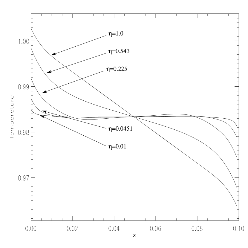
Figure 9: Vertical profile of the horizontally averaged temperature at late times in runs with various initial magnetic field strengths (runs A1-A5). As the stability parameter, $\eta$, decreases, the saturated state asymptotically approaches an isothermal profile. States with sufficiently strong initial magnetic fields never saturate to an isothermal state.

The second effect observed from the variation of the magnetic field strength is the degree of saturation obtained in terms of an isothermal temperature profile. Figure 9 shows various saturated temperature profiles taken at the same time but with different stability parameters. Where magnetic tension dominates, the temperature profiles have evolved less from the initial conditions. As the influence of the magnetic field decreases, the temperature profiles become more isothermal. The profiles of simulations with higher magnetic field would not continue to evolve if the simulation were given more time, as the instability is simply turned off before its free energy source is completely used. Essentially, the MTI reduces the thermal gradient, the source of free energy, and amplifies the magnetic field (increases the Alfvén velocity) until the two terms of Equation 17 balance. A new, stable macroscopic thermodynamic equilibrium is then established.

5 Non-Linear Regime of the Conducting Boundary Conditions

With adiabatic boundary conditions, there is a limited amount of free energy available to the system, and once saturation occurs, the motions decay away and a new vertical equilibrium corresponding to an isothermal atmosphere (if $\eta\ll 1$) is established. With conducting boundary conditions, however, an isothermal profile across the domain can never be achieved. Free energy to drive motions can always be tapped from the boundaries; therefore, we might expect that sustained convection and turbulence are possible in this case. To test these expectations, we have performed a series of simulations of the nonlinear evolution of the MTI using conducting boundary conditions.

Table 2 is a list of all runs using conducting boundary conditions discussed in this paper. As a fiducial model, we consider a simulation with zero initial net magnetic flux, run N3, which is perturbed with multiple modes. An analogous case (Run N2) was considered in §4.2 for the adiabatic boundary condition. Figure 10 shows the evolution of the magnetic field at various times. The linear evolution is not shown, but is quite similar to the adiabatic, multimode case (see Figure 7). After the system reaches a quasi-equilibrium, bubbles of magnetic field emanate from the vertical boundaries and penetrate to the center of the atmosphere. These bubbles are reminiscent of nucleate boiling familiar from fluid mechanics (Incropera & DeWitt, 1996). One can observe the characteristic Kelvin-Helmholtz rolls on these bubbles. This boiling “steady-state” behavior is reached after approximately 2,000 sound-crossing times as reflected by the plot of the magnetic and kinetic energies shown in Figure 11. It is clear that after an initial spike some kinetic energy remains in the system, driven by the heat flux at the boundaries.

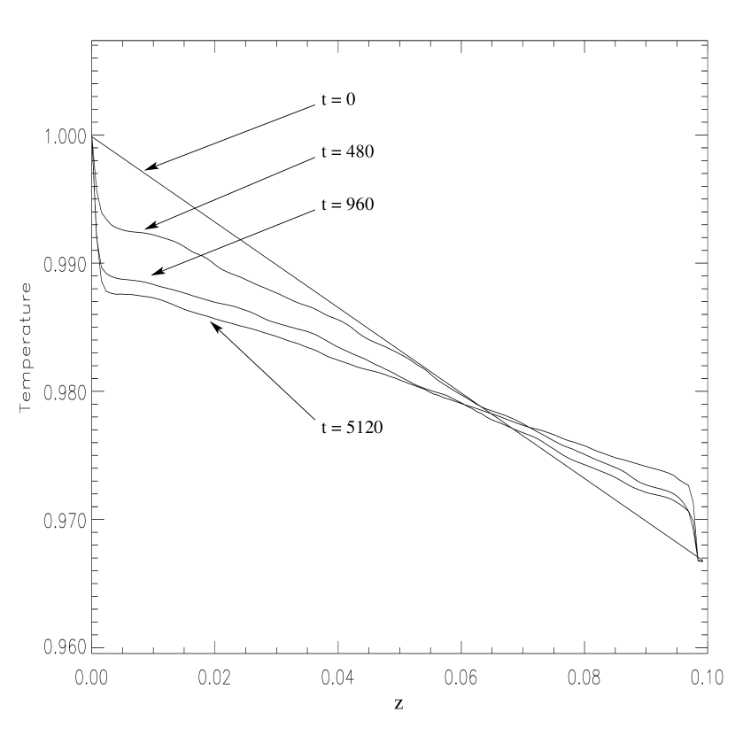
Figure 12: Vertical profiles of the horizontally averaged temperature at various times in Run N3. A narrow thermal boundary layer develops, while the interior saturates to a more isothermal profile than the initial state. The width of the boundary layers is resolution-dependent.

The system is driven towards a more isothermal state with large boundary layers at the upper and lower surfaces of the simulation (Figure 12). Resolution studies show that as the simulation resolution is increased ($128^{2}$ is shown) the boundary layers shrink, and the interior region becomes closer to isothermal. We conclude that the fluid motion observed at late times is driven by the MTI in an unresolved thermal boundary at the top and bottom edges of the domain. The resolution dependence of the boundary layer makes it difficult to determine the efficiency of heat transport by the magnetothermal instability in this case.

In fact, the resulting vertical structure which emerges is not likely to be applicable to most astrophysical systems. The use of a solid reflecting wall kept at a constant temperature leads to a thin thermal boundary layer, and the structure of this layer determines the physics. In a real atmosphere, we expect the size of this boundary layer to be set by the size of the transition region from isotropic to anisotropic conduction. This will be explored further in §5.2, where we use isotropic conduction to introduce resolved layers near the boundaries which are stably stratified with respect to the Balbus criterion. This modification avoids the formation of thermal boundary layers at the wall.

5.1 Dependence of the Saturated State on Isotropic Conduction

As was shown in §3.3, the linear growth rate of the MTI is damped by the addition of isotropic conduction. This behavior is similar in many respects to that of the strong magnetic field case. The saturated state is also dependent upon the anisotropy parameter, $Q$. Figure 13 shows the horizontally averaged temperature profiles at the time of saturation as calculated from runs I1-I4. As can be seen, even a modest amount of isotropic conduction, $Q=0.9$, is able to significantly reduce the saturation level of the instability. When the isotropic conduction is strong, $Q=0.1$, the temperature profile only marginally deviates from the initial condition. The driving term of the instability is reduced by the anisotropic fraction, thus, causing saturation after much less growth. In addition, the saturation magnetic energy density, $\Delta$, [Eq. (27)] scales monotonically with $Q$, asymptotically reaching its maximum value for purely anisotropic conduction.

5.2 Models with Convectively Stable layers

A more realistic boundary condition is implemented by establishing an atmosphere with layers at the top and bottom that are stable according to the Balbus criterion. This is accomplished by transitioning slowly from pure anisotropic conduction to isotropic conduction at the boundaries of the domain. We have performed a simulation, Run N4, with a domain $L_{x}=0.1$, $L_{z}=0.2$ and a resolution of 100x250. The average horizontal sound crossing time is slightly higher than the previous studies with $\bar{\tau_{s}}\approx 7.88\times 10^{-2}$. Multiple modes are seeded with Gaussian noise smoothed towards the vertical boundaries. The total conductivity is $\chi_{tot}=10^{-4}$, while the isotropic and anisotropic conduction coefficients $\chi_{R}$ and $\chi_{C}$ are chosen such that the anisotropy parameter $Q$ is

$$Q(z)=\left\{\begin{array}[]{ll}\frac{5}{L_{z}}\left(z-\frac{L_{z}}{5}\right)&\frac{L_{z}}{5}\leq z\leq\frac{2L_{z}}{5}\\ 1&\frac{2L_{z}}{5}\leq z\leq\frac{3L_{z}}{5}\\ 1-\frac{5}{L_{z}}\left(z-\frac{3L_{z}}{5}\right)&\frac{3L_{z}}{5}\leq z\leq\frac{4L_{z}}{5}\\ 0&\textrm{otherwise.}\end{array}\right.$$ (28)

Since $\chi_{C}=Q(z)\chi_{tot}$ and $\chi_{R}=(1-Q(z))\chi_{tot}$, the conduction is purely isotropic near the boundaries, purely anisotropic in the center, and linearly interpolated in between.

The magnetic field strength is initialized to follow the same vertical profile, so that $B_{x}(z)=B_{0}Q(z)$, with $B_{0}/\sqrt{4\pi}=10^{-4}$. With this definition, the magnetic field is non-zero only in those regions that are at least slightly unstable by the Balbus criterion. We can track the mixing of the stable and unstable layers by following the location of the field, since in ideal MHD the field is “frozen in” to the fluid.

Figure 14 shows the $x$ and $z$ components of the magnetic and kinetic energy averaged over the domain in Run N4. This plot is not much different than the previous driven case Run N3 (Figure 11), except the magnetic field does not decay in time due to the presence of a net magnetic flux. The background temperature profile only deviates slightly from the initial condition, indicating a fairly steady state. The most interesting insights come from examining the field lines at several different times as shown in Figure 15. The far left and middle left plots show the unstable central region in the linear and early non-linear phases. By the middle right plot, however, plumes driven by the MTI have penetrated the convectively stable region, as evidenced by the magnetic field plume with Kelvin-Helmholtz roll. At a much later time, when the system is essentially in steady state, much of the magnetic field has been stored in the stable region through convective overshoot. The phenomena of penetrative convection and overshooting has been thorougly studied in the magnetoconvection of stellar atmospheres, and it is likely this phenomenon is universal (Tobias, et al., 2001; Brummell, Clune, & Toomre, 2002). In three dimensions this behavior could have important implications for a magnetic dynamo.

A further diagnostic is the comparison of the magnitude of each component of the horizontally-averaged heat fluxes at different heights. In addition to the Coulombic (equation 6) and radiative (equation 7) heat fluxes, we define an advective heat flux,

$$\mathbf{Q_{adv}}\equiv\mathbf{V}\epsilon,$$ (29)

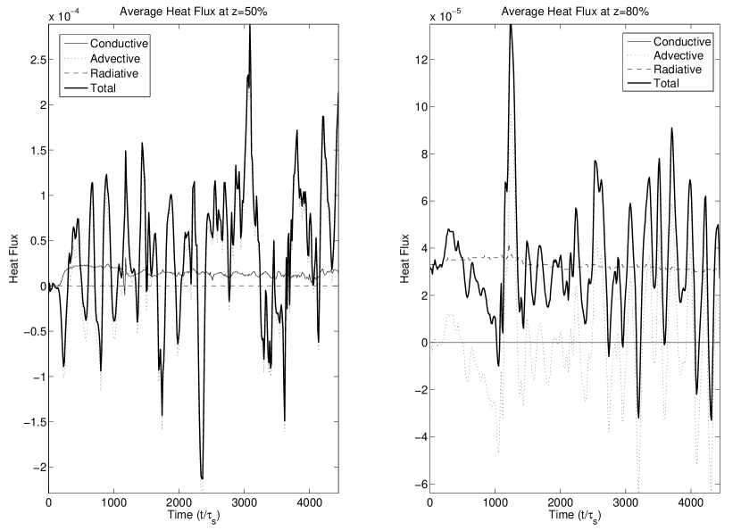
Figure 16: Time evolution of the horizontally averaged heat flux at the midplane and 80% height of the simulation domain in Run N4. The total heat flux (thick solid line) is subdivided into Coulombic (thin solid line), radiative (dashed lined), and advective (dotted line) components. The instantaneous advective heat flux generally is the dominant component of the total heat flux, particularly at the midplane.

where, $\mathbf{V}$, is the fluid velocity, and $\epsilon=p/(\gamma-1)$, is the internal energy. Figure 16 plots the time evolution of the vertical components of these three heat fluxes and the total heat flux at the midplane, and at 80% of the height of the domain in Run N4. At the former height only anisotropic conduction is present, while at the latter only isotropic conduction is present. At the midplane the oscillatory advective heat flux is clearly dominant at any given instant in time; however, averaged in time the advective heat flux contributes roughly $2/3$ of the total heat flux. The Coulombic flux, which is relatively constant in time, contributes the remaining $1/3$. This fact is evident in Table 3, which lists the time- and horizontally-averaged total heat fluxes in the vertical direction at three different vertical heights.

To consider the heat conduction efficiency of the instability, we compare it to the expected heat flux across the simulation domain for pure uniform isotropic conductivity, namely $Q_{0}\approx 3.33\times 10^{-5}$. The time-averaged heat conduction at the midplane is $\left<Q_{tot,50\%}\right>\approx 3.54\times 10^{-5}$, which indicates that the instability transports the entire applied heat flux. Thus, we conclude that the MTI efficiently transports heat flux in this two-dimensional case.

6 Summary and Potential Applications

Given an atmosphere with $dS/dZ<0$ and $N^{2}>0$, one would expect it to be stable to convection. Yet, if the density is low enough such that anisotropic heat conduction along magnetic field lines is important, the atmosphere is in fact convectively unstable, and it will establish a radically different hydrostatic equilibrium using the free energy provided by the initial temperature gradient. We refer to the new stability criterion in this case as the Balbus criterion, and the convective instability that results as the magnetothermal instability.

Using time-dependent MHD simulations, we have verified the linear properties of the MTI predicted by Balbus (Balbus, 2000). The growth rates and Balbus criterion measured from the simulations agree well with linear theory. In the nonlinear regime, the instability saturates as an isothermal atmosphere. Steady convective turbulence can be driven if a fixed temperature difference is maintained across the upper and lower boundaries. In this case, the advective heat flux carried by fluid motions is larger than the conductive heat flux by a factor of two. The amplitude of the conductivity is important only in establishing the most unstable wavelength. For purely anisotropic conduction, the maximum growth rate is independent of the conductivity. Thus, our simulations show that if the Balbus criterion is satisfied, unstable modes will produce vigorous motions and a significant heat flux, even if the conductivity is very small, and conduction times very long. We have also used simulations to study the effects of magnetic tension and isotropic conduction on the saturated state; in both cases the MTI saturates before an isothermal profile is established.

There are several important directions for future studies. Three dimensional simulations of driven, steady convection that explore the heat fluxes and dynamo action in the MTI will be reported in a future paper. In addition, applications of the MTI to specific astrophysical systems are warranted. Two potential applications are of obvious and immediate interest. The first is to explore whether the MTI can help explain the nearly isothermal temperature profiles observed in the outer regions of x-ray emitting gas in clusters of galaxies (Fabian, 1994). In this case, anisotropic ion viscosity (which has been ignored in this study) may also be important. The second is to understand the effect of the MTI on radiatively inefficient accretion flows. In particular, there is much interest in the transport properties of turbulence driven by convection (Narayan, Mahadevan, & Quataert, 1998; Stone, Pringle, & Begelman, 1999; Narayan, Igumenschev, & Abramowicz, 2000; Quataert & Gruzinov, 2000) versus the MRI (Stone & Pringle, 2001; Hawley, Balbus, & Stone, 2001; Balbus & Hawley, 2002; Hawley & Balbus, 2002) in such flows. However, since for diffuse plasmas the appropriate stability criterion is not the Høiland but rather the Balbus criterion, it is important to investigate how this changes the structure of the flow.

Appendix A Anisotropic Heat Conduction

The heat conduction equation for Coulombic conduction is

$$\frac{3}{2}\frac{Pd\ln P\rho^{-5/3}}{dt}=-\mathbf{\nabla}\cdot\mathbf{Q}=\mathbf{\nabla}\cdot[\mathbf{\hat{b}}(\chi_{C}\mathbf{\hat{b}}\cdot\mathbf{\nabla}T)],$$ (A1)

where $\mathbf{\hat{b}}$ is a unit vector in the direction of the magnetic field. In Cartesian coordinates, the right hand side may be written as

$$\chi_{C}\left\{\frac{\partial}{\partial x}\left[\hat{b}_{x}\left[\hat{b}_{x}\frac{\partial T}{\partial x}+\hat{b}_{y}\frac{\partial T}{\partial y}\right]\right]+\frac{\partial}{\partial y}\left[\hat{b}_{y}\left[\hat{b}_{y}\frac{\partial T}{\partial x}+\hat{b}_{y}\frac{\partial T}{\partial y}\right]\right]\right\},$$ (A2)

where $\hat{b_{x}}=B_{x}/[B_{x}^{2}+B_{y}^{2}]$ is the $x$-component of the magnetic field normalized by the magnitude of $B$. In order to develop a finite-difference representation of equation A2, note that the Athena code stores the magnetic field at cell faces and the temperature at cell centers. Thus, the second $x-$derivatives can be differenced as:

$$\frac{\partial}{\partial x}\left(\hat{b}_{x}^{2}\frac{\partial T}{\partial x}\right)=\frac{\hat{b}_{x,i+1/2,j}^{2}\left(T_{i+1,j}-T_{i,j}\right)-\hat{b}_{x,i-1/2,j}^{2}\left(T_{i,j}-T_{i-1,j}\right)}{\left(\Delta x\right)^{2}},$$ (A3)

and similarly for the second $y-$derivative. The cross derivatives are considerably more complicated, requiring a 3x3 difference molecule to incorporate the change in the direction of the magnetic field across a cell. In addition, the mixed derivatives are written in a symmetrized way, so that the heat transport is manifestly conservative. For example,

$$\frac{\partial}{\partial x}\left(\hat{b}_{x}\hat{b}_{y}\frac{\partial T}{\partial y}\right)=\frac{\hat{b}_{x,i+1/2,j}\hat{b}_{y,i+1/2,j}\left[\left(T_{i+1,j+1}-T_{i+1,j-1}\right)+\left(T_{i,j+1}-T_{i,j-1}\right)\right]}{4\Delta x\Delta y}$$ (A4)

$$-\frac{\hat{b}_{x,i-1/2,j}\hat{b}_{y,i-1/2,j}\left[\left(T_{i-1,j+1}-T_{i-1,j-1}\right)+\left(T_{i,j+1}-T_{i,j-1}\right)\right]}{4\Delta x\Delta y}.$$

The difference formula are implemented in an external module to the MHD integrator in Athena. The two are combined using operator splitting—that is equation A1 is updated after a full timestep of the MHD equations. Sub-cycling is used when the stability limit for the timestep used in the conduction module is smaller than the timestep resulting from the MHD algorithm.

To test the accuracy of the diffusion modeule, we have computed the diffusion of a Gaussian profile of temperature in a medium with uniform thermal conductivities. In our tests with straight magnetic field lines at an arbitrary angle to the grid the above finite differencing yields fractional L2 error norms that are $O(10^{-8})$, independent of angle.

More complex tests involve anisotropic conduction along curved magnetic field lines. One of the more challenging test problems we devised is the conduction of heat along circular magnetic field lines. Specifically the problem is defined on a domain spanning $\{x,z\}\in\{(-1,-1)...(1,1)\}$. A circular heat pulse is initialized in a region of an annulus defined as

$$T(r,\theta)=\left\{\begin{array}[]{ll}T^{*}&\textrm{if}\ (0.5\leq r\leq 0.7)\textrm{ and }(\frac{11\pi}{12}\leq\theta\leq\frac{13\pi}{12})\\ T_{0}&\textrm{otherwise;}\end{array}\right.$$ (A5)

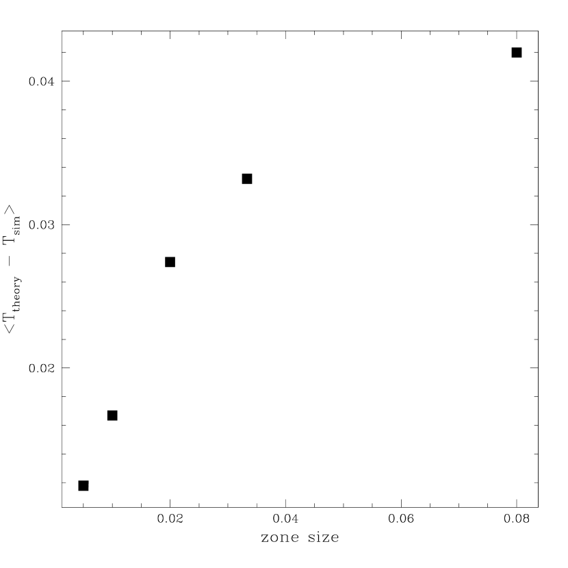
Figure 17: The convergence of the average error with resolution for the circular conduction test problem.

where in our simulation $T^{*}=12.0$, $T_{0}=10.0$, and $\chi_{\parallel}=0.01$. Figure 17 shows the quantitative convergence of the L1 error. At low resolution a large fraction of the error arises simply from the discretization of a curvilinear problem to a Cartesian domain.

From conservation of energy we can estimate the effective cross-field diffusion coefficient. Recall Fourier’s law of conduction for a heat flux, $q^{\prime\prime}=k\partial T/\partial x$ in units of $[W/m^{2}]$. We can calculate the total energy passing through an area as

$$\int_{0}^{t}\dot{E}(t^{\prime})dt^{\prime}=\int_{0}^{t}\chi_{\perp}\frac{\partial T(t^{\prime})}{\partial x}A_{\perp}dt^{\prime},$$ (A6)

where $A_{\perp}$ is the cross-sectional area. Take the 100x100 resolution case as a canonical example since it was used as our minimum resolution. At time $t=200$ when the annulus is essentially isothermal, the net heat that has leaked from the annulus is $\Delta E=0.041$. By doing an order of magnitude estimate on equation A6 we find that $\chi_{\perp}\sim 4\times 10^{-6}$  implying that the ratio $\chi_{\perp}/\chi_{\parallel}\sim 10^{-3}-10^{-4}$. As we have demonstrated previously, the instability is insensitive to isotropic conduction of this order of magnitude.

Table 1: Properties of Runs with Adiabatic Boundaries

Run	$\chi_{C}$	$\chi_{R}$	$B_{0}/\sqrt{4\pi}$	$\eta$	Flux	Resolution	Mode
N1	$1\times 10^{-4}$	0.0	$5.0\times 10^{-4}$	$2.82\times 10^{-3}$	+	$(100)^{2}$	Single
N2	$1\times 10^{-4}$	0.0	$5.0\times 10^{-4}$	$2.82\times 10^{-3}$	-	$(128)^{2}$	Multi
A1	$1\times 10^{-4}$	0.0	$9.42\times 10^{-2}$	1.0	+	$(100)^{2}$	Single
A2	$1\times 10^{-4}$	0.0	$6.94\times 10^{-2}$	0.543	+	$(100)^{2}$	Single
A3	$1\times 10^{-4}$	0.0	$4.47\times 10^{-3}$	0.225	+	$(100)^{2}$	Single
A4	$1\times 10^{-4}$	0.0	$2.0\times 10^{-3}$	$4.51\times 10^{-2}$	+	$(100)^{2}$	Single
A5	$1\times 10^{-4}$	0.0	$9.42\times 10^{-4}$	$1.0\times 10^{-2}$	+	$(100)^{2}$	Single

Table 2: Properties of Runs with Conducting Boundaries

Run	$\chi_{C}$	$\chi_{R}$	$B_{0}/\sqrt{4\pi}$	$\eta$	Flux	Resolution	Mode
N3	$1\times 10^{-4}$	0.0	$5.0\times 10^{-4}$	$2.82\times 10^{-3}$	-	$(128)^{2}$	Multi
I1	$1\times 10^{-4}$	0.0	$5\times 10^{-4}$	$2.82\times 10^{-3}$	+	$(100)^{2}$	Single
I2	$9\times 10^{-5}$	$1\times 10^{-5}$	$5\times 10^{-4}$	$3.13\times 10^{-3}$	+	$(100)^{2}$	Single
I3	$5\times 10^{-5}$	$5\times 10^{-5}$	$5\times 10^{-4}$	$5.63\times 10^{-3}$	+	$(100)^{2}$	Single
I2	$1\times 10^{-5}$	$9\times 10^{-5}$	$5\times 10^{-4}$	$2.82\times 10^{-2}$	+	$(100)^{2}$	Single

Table 3: Time-Averaged Vertical Heat Fluxes in Run N4 (see §5.2)

Height	$\left<Q_{C}\right>$	$\left<Q_{R}\right>$	$\left<Q_{Adv}\right>$	$\left<Q_{tot}\right>$
20%	0	$3.41\times 10^{-5}$	$-6.23\times 10^{-6}$	$2.79\times 10^{-5}$
50%	$1.39\times 10^{-5}$	0	$2.15\times 10^{-5}$	$3.54\times 10^{-5}$
80%	0	$3.30\times 10^{-5}$	$-2.97\times 10^{-7}$	$3.27\times 10^{-5}$

Figure 1: Solutions of the MTI dispersion relation in the weak field limit for an atmosphere with $d\ln T/d\ln S=-3.$ The axes are normalized to the local Brunt-Väisälä frequency, $N$. The crosses are growth rates measured from simulations (see §3.1).

Figure 2: The effect of magnetic tension on the MTI. The growth rate $\sigma$ decreases dramatically as magnetic tension increases, i.e. the stability parameter $\eta=k^{2}V_{A}^{2}/\sigma^{2}_{\rm max}$ increases. The transition from stable to unstable is marked by a vertical dashed line, and the maximum growth rate in the limit of weak magnetic field $\sigma_{\rm max}$ is marked by a horizontal dashed line.

Figure 3: The effect of isotropic conductivity. Holding the total conductivity $\chi_{\mathrm{tot}}$ and all other quantities fixed, the anisotropic fraction, $Q$, is varied. As $Q$ approaches 1.0, conduction is purely anisotropic, and the growth rate reaches an asymptotic value. As the conduction becomes more isotropic, i.e. $Q$ approaches zero, the instability is quenched. The solid line marked ’theory’ is the unstable branch in the solutions of equation 16

Figure 4: Snapshots of the magnetic field lines in run N1 at various times during the evolution of the instability. (upper left) Inititial condition; (upper right) Linear phase; (lower left) Non-linear phase; (lower right) Saturated state.

Figure 5: Time evolution of the components of the volume averaged magnetic energy and kinetic energy in run N1. The time axis is non-dimensionalized by the sound crossing time, $\tau_{S}$.

Figure 6: Vertical profile of the horizontally-averaged temperature profile in run N1 at various times. The initial state is a monotonically decreasing temperature profile with respect to height, and the final state is isothermal.

Figure 7: Snapshots of the magnetic field lines at various times during the evolution of the MTI in run N2. The structure is more complex than the single-mode case. (upper left) Initital condition; (upper right) Linear phase; (lower left) Non-linear phase; (lower right) Saturated state.

Figure 8: Time evolution of the components of the volume averaged magnetic energy and the kinetic energy in run N2. The magnetic field decays in time due to the anti-dynamo theorem.

Figure 10: Snapshots of the magnetic field lines at various times during the evolution of run N3. (upper left) The initial magnetic field. (uper right) Early non-linear growth is marked by highly complex field geometry, reconnection, and generation of vorticity. The bottom plots show narrow plumes generated at the boundaries. A thermal boundary layer is evident at the upper and lower surfaces.

Figure 11: Time evolution of the components of the volume averaged magnetic energy and the kinetic energy in run N3. The magnetic field decays in time, but the kinetic energy continues to fluctuate due to the plumes generated at the boundaries.

Figure 13: Vertical profiles of the horizontally averaged temperature at late times with various values of $Q=\chi_{C}^{\prime}/\chi^{\prime}$, the fraction of anisotropic conductivity. The initial condition is denoted ‘IC’. It is clear that even a modest amount of isotropic conductivity significantly modifies the saturated state of the MTI.

Figure 14: Time evolution of the components of the volume averaged magnetic and kinetic energy for Run N4.

Figure 15: Snapshots of the magnetic field in Run N4. (far left) Early linear phase; (middle left) early non-linear phase. (middle right) The MTI drives penetrative convection into the stable layers, and at late times (far right) magnetic flux is pumped into the stable layers.

References

- Balbus & Hawley (1998) Balbus, S. A., & Hawley J. F. 1998, Rev. Mod. Phys., 70, 1
- Balbus (2000) Balbus, S. A. 2000, ApJ, 534, 420
- Balbus (2001) Balbus, S. A. 2001, ApJ, 562, 909
- Balbus & Hawley (2002) Balbus, S. A., Hawley, J. F. 2002, ApJ, 573, 749
- Balbus (2004) Balbus, S. A. 2004, ApJ, 616, 857
- Braginskii (1965) Braginskii, S. I. 1965, in Reviews of Plasma Physics, Vol. 1, ed. M. A. Leontovich (New York: Consultants Bureau), 205
- Brummell, Clune, & Toomre (2002) Brummell, N.H., Clune, & T.L., Toomre, J. 2002, ApJ, 570, 825
- Cowling (1934) Cowling, T.G. 1934, MNRAS, 94, 39
- Fabian (1994) Fabian, A. C. 1994, ARA&A, 32, 277
- Gardiner & Stone (2005) Gardiner, T. & Stone, J. 2005, J. Comp. Phys., 205, 509
- Hammett & Perkins (1990) Hammett, G. W. & Perkins, F. W. 1990, Phys. Rev. Lett., 64, 3019
- Hawley, Gammie, & Balbus (1995) Hawley, J. F., Gammie, F., & Balbus, S. A. 1995, ApJ, 440, 742
- Hawley, Balbus, & Stone (2001) Hawley, J. F., Balbus, S. A., & Stone, J. M. 2001, ApJ, 554, L49
- Hawley & Balbus (2002) Hawley, J. F. & Balbus, S. A. 2002, ApJ, 573, 738
- Incropera & DeWitt (1996) Incropera, F. & DeWitt, D. 1996, Fundamentals of Heat and Mass Transfer (4th ed.; New York:Wiley)
- Narayan, Igumenschev, & Abramowicz (2000) Narayan, R., Igumenschev, I.V., & Abramowicz, M.A. 2000, ApJ, 539, 798
- Narayan, Mahadevan, & Quataert (1998) Narayan, R., Mahadevan, R., Quataert, E. 1998, in Theory of Black Hole Accretion Disks, ed. M.A. Abramowicz, et al (Cambridge: Cambridge University Press), 148
- Quataert, Hammett, & Dorland (2002) Quataert, E., Dorland, W., & Hammett, G. W. 2002 ApJ, 577, 524
- Quataert & Gruzinov (2000) Quataert, E., Gruzinov, A. 2000, ApJ, 539, 809
- Sharma, Hammett, & Quataert (2003) Sharma, P., Hammett, G., Quataert, E. 2003, ApJ, 596, 1121
- Spitzer (1962) Spitzer, L. 1962, Physics of Fully Ionized Gases (New York: Wiley)
- Stone & Pringle (2001) Stone, J. M. & Pringle, J. E. P. 2001,MNRAS, 322, 461
- Stone, Pringle, & Begelman (1999) Stone, J. M., Pringle, J. E. P. , & Begelman, M. C. 1999, MNRAS, 310, 1002
- Tobias, et al. (2001) Tobias, S. M., et al. 2001, ApJ, 549, 1183
- Zakamska & Narayan (2003) Zakamska, N. L., & Narayan, R. 2003, ApJ, 582, 162