The Detectability of Pair-Production Supernovae at ${z\lower 2.15277pt\hbox{$\;\buildrel<\over{\sim}\;$}6}$

Abstract

Nonrotating, zero metallicity stars with initial masses $140\lower 2.15277pt\hbox{$\;\buildrel<\over{\sim}\;$}M_{\star}\lower 2.15277pt\hbox{$\;\buildrel<\over{\sim}\;$}260\,\,{\rm M_{\odot}}$ are expected to end their lives as pair-production supernovae (PPSNe), in which an electron-positron pair-production instability triggers explosive nuclear burning. Interest in such stars has been rekindled by recent theoretical studies that suggest primordial molecular clouds preferentially form stars with these masses. Since metal enrichment is a local process, the resulting PPSNe could occur over a broad range of redshifts, in pockets of metal-free gas. Using the implicit hydrodynamics code KEPLER, we have calculated a set of PPSN light curves that addresses the theoretical uncertainties and allows us to assess observational strategies for finding these objects at intermediate redshifts. The peak luminosities of typical PPSNe are only slightly greater than those of Type Ia, but they remain bright much longer ($\sim$ 1 year) and have hydrogen lines. Ongoing supernova searches may soon be able to limit the contribution of these very massive stars to $\lower 2.15277pt\hbox{$\;\buildrel<\over{\sim}\;$}1\,$% of the total star formation rate density out to $z\approx 2,$ which already provides useful constraints for theoretical models. The planned Joint Dark Energy Mission satellite will be able to extend these limits out to $z\approx 6$.

1. Introduction

Determining the cosmological evolution of the elements and elucidating the processes responsible for their creation are key aspects of understanding the history of the universe. A wide spread in abundances is observed in stars, but the lowest metallicity galaxies studied so far are enriched to substantial values of $\sim 0.02Z_{\odot}$ (e.g., Searle & Sargent 1972), and the diffuse medium in galaxy clusters is enriched to levels above 1/3 $Z_{\odot}$ (e.g., Renzini 1997). Similarly, quasar absorption line studies have uncovered heavy elements in even the lowest-density regions of the intergalactic medium (IGM) (e.g., Schaye et al. 2003; Aracil et al. 2004) at levels that are roughly constant out to the highest redshifts probed (Songaila 2001; Pettini et al. 2003). And though direct observations of metal-poor halos stars have uncovered a number of unusual abundance patterns (e.g., Ryan, Norris, & Beers 1996; Christlieb et al. 2002; Cayrel et al. 2004), no metal-free star has been detected to date.

Thus a clear signature of the transition from a metal-free to an enriched universe has so far remained unobserved. Furthermore, there are good reasons to believe that this transition may have marked a drastic change in the characteristics of star formation. Recent theoretical studies have shown that collapsing primordial clouds fragmented into clumps with typical masses $\sim 10^{3}\,{\rm M_{\odot}}$ (e.g., Nakamura & Umemura 1998; Abel, Bryan, & Norman 2000; Bromm et al. 2001) and that accretion onto proto-stellar cores within these clouds was very efficient (Ripamonti et al. 2002; Tan & McKee 2004). The implication is that the initial mass function (IMF) of metal-free “Population III” stars may have been biased to higher masses than observed today.

Since only a trace level of heavy elements will drastically increase fragmentation, the formation of very massive stars (VMS) is unlikely beyond a “critical metallicity” of $Z_{\rm crit}\sim 10^{-4}$ (e.g., Schneider et al. 2002; Bromm & Loeb 2003). This means that the metals produced by the first few supernovae (SNe) were sufficient to halt very massive star formation, implying that this mode may have only operated at extremely high-redshifts $z\lower 2.15277pt\hbox{$\;\buildrel>\over{\sim}\;$}15$ (e.g., Mackey, Bromm, & Hernquist 2003). Yet, such simple estimates ignore the substantial propagation times necessary for heavy elements to be mixed into pristine material. In fact, more detailed analyses show that it is almost impossible to raise the IGM metallicity above $Z_{\rm crit}$ in a homogeneous way (Scannapieco, Schneider, & Ferrara 2003, hereafter SSF03). Thus primordial metal enrichment was essentially a local process, which began in the densest “high-sigma” regions and gradually spread into to the more common lower-density regions as time progressed. This inhomogeneous distribution parallels models of further IGM enrichment by second-generation objects (e.g., Scannapieco, Ferrara, & Madau 2002; Theuns et al. 2002; Fujita et al. 2004; Cen, Nagamine & Ostriker 2004) and raises the possibility that metal-free star formation may extend well into the observable range, in pockets of gas where metals have not yet propagated.

Such primordial star-forming regions would naturally be isolated. Similarly, metal-free objects would tend to be just large enough for gravitational collapse to overcome the IGM thermal pressure, but small enough to have no direct progenitors above a cosmological Jeans mass. After reionization, such pristine star formation would be fundamentally different than that taking place in minihalos at very high redshifts, which depends sensitively on the presence of initial $H_{2}$ (e.g., O’Shea et al. 2005). In small objects, molecular hydrogen is easily photodissociated by 11.2-13.6 eV photons, to which the universe is otherwise transparent. Thus the emission from the first stars quickly destroyed all avenues for cooling by molecular line emission (Dekel & Rees 1987; Haiman, Rees, & Loeb 1997; Ciardi, Ferrara, & Abel 2000). This quickly raised the minimum virial temperature necessary to cool effectively to approximately $10^{4}$ K, although the precise value of this transition is the subject of debate (e.g., Glover & Brand 2001 Yoshida et al. 2003) and is somewhat dependent on the level of the high-redshift X-ray background (Haiman, Rees, & Loeb 1996; Oh 2001; Machack, Bryan, & Abel 2003).

Later metal-free star formation is much more straightforward, and is confined to halos with $T_{\rm vir}\geq 10^{4}$ K. In this case efficient atomic line cooling establishes a dense locally-stable disk, within which non-equilibrium free electrons catalyze $H_{2}$. Unlike in less massive halos, $H_{2}$ formation in these objects is largely impervious to feedback from external UV fields, due to the high densities achieved by atomic cooling (Oh & Haiman 2002). As discussed in SSF03, these lonely regions of late primordial star formation may have already been detected as a subgroup of high-redshift Lyman-alpha emitters, although distinguishing these objects from Population II stars is extremely difficult (Dawson et al. 2004).

In this investigation we explore an alternative approach to search for such VMS: the direct detection of the resulting SNe. While many of the $M_{\star}\geq 100\,{\rm M_{\odot}}$ stars would have died forming black holes, progenitors within the $140-260\,{\rm M_{\odot}}$ mass range end their lives in tremendously powerful pair-production supernovae (PPSNe). In these SNe, $e^{+}e^{-}$ pair creation softens the equation state at the end of central carbon burning, leading to rapid collapse, followed by explosive burning up to the iron group (e.g., Ober, El Eid, & Fricke 1983; Bond, Arnett, Carr 1984; Heger & Woosley 2002, hereafter HW02). The more massive the star, the higher the temperature at bounce and the heavier the elements that are produced by nuclear fusion. In all cases, the star is completely disrupted and both the ejection energies ($\sim 3-100\times 10^{51}$ ergs) and masses ($140-260\,{\rm M_{\odot}}$) are enormous, leading to observed properties qualitatively different from those of Type-Ia and typical core collapse SNe. In turn, these properties, such as bright UV colors, allow for efficient intermediate-redshift searches for very massive star formation.

Recently, Wise & Abel (2005) studied the feasibility of detecting PPSNe at $z\sim 20$ with the James Webb Space Telescope, using extremely approximate lightcurves with luminosities that were taken to be proportional to the total ⁵⁶Ni mass. A similar study was carried out by Weinmann & Lilly (2005), who also estimated number counts at $z=5$ using a single light curve that was taken from Heger et al. (2002), which unfortunately contained a normalization error. Limited studies of lightcurves from PPSNe have also been carried out by Woosley & Weaver (1982), who considered progenitors with only two masses and found features similar to those described below, and by Herzig et al. (1990) who modeled the disruption of a 61 $\,{\rm M_{\odot}}$ Wolf-Rayet star, generating a relatively faint SN. Here we use the KEPLER code to directly construct a suite of PPSN models that addresses the range of theoretical possibilities and accounts for the detailed physical processes involved up until the point at which the SN becomes optically thin. These curves allow us to identify the properties that most distinguish PPSNe from Type Ia and core collapse SNe, and discuss their detectability at $z\lesssim 6$ in current and future surveys.

The outline of this paper is as follows. In §2 we use the implicit hydrodynamical code KEPLER to construct a suite of detailed PPSN progenitor models. In §3 we generate simulated spectra and lightcurves from these models, highlighting the key features that distinguish PPSNe from other SNe. In §4 we apply these lightcurves to determine the constraints on PPSNe obtainable by existing and planned SNe searches. In §5 we discuss the properties of the most likely environments of PPSNe, and we summarize our results in §6.

Table 1Properties of PPSN progenitor models

Model	$M_{\rm He}$ ($\,{\rm M_{\odot}}$)	$M_{\rm N}$ ($\,{\rm M_{\odot}}$)	$M_{{}^{56}{\rm Ni}}$ ($\,{\rm M_{\odot}}$)	$R$ ($10^{13}{\rm cm}$)	${\cal E}_{\rm kin}$ ($10^{51}{\rm ergs}$)
150-W	70	3.5(-4)	4.2(-2)	3.9	6.9
150-I	46	1.1(-4)	6.3(-2)	16	9.2
150-S	49	0.86	8.6(-2)	26	8.5
200-W	97	2.7(-6)	3.3	0.68	29.5
200-I	58	8.0(-6)	5.1	2.8	36.5
200-S	89	0.34	2.2	29	29.1
200-S2	78	4.75	0.82	20	18.7
250-W	123	3.1(-6)	6.2	0.58	47.2
250-I	126	9.1(-6)	32	4.0	76.7
250-S	113	1.34	24.5	26	64.6

2. Models of Pair-Production Supernovae

The progenitors of PPSNe are confined to a range of initial masses that are large enough to collapse via the pair-production instability, but small enough for this collapse to be reversed by nuclear burning. In the non-rotating case, these limits are clearly defined and well understood numerically (Ober, El Eid, & Fricke 1983; HW02; Heger et al. 2003). In stars above $\sim 100\,{\rm M_{\odot}}$, after central helium burning, the core reaches a sufficiently high temperature and entropy to produce $e^{+}e^{-}$ pairs, converting some of the internal energy of the gas into rest mass, which softens the equation of state to an adiabatic index below the critical value of 4/3 (Barkat, Rakavy, & Sack 1967; Bond, Arnett, & Carr 1984). The result is a runaway collapse that leads to explosive burning in the carbon-oxygen core. For stars with initial masses more than about 140 $\,{\rm M_{\odot}},$ the energy released is sufficient to completely disrupt the star.

A shock moves outward from the edge of the core, initiating the supernova outburst when it reaches the stellar surface. Just above the 140 $\,{\rm M_{\odot}}$ limit, weak silicon burning occurs and only trace amounts of radioactive ⁵⁶Ni are produced. It is this ⁵⁶Ni that powers the late-time supernova light curves. The amount of ⁵⁶Ni produced increases in larger progenitors, and in 260 $\,{\rm M_{\odot}}$ progenitors up to 50 $\,{\rm M_{\odot}}$ may be synthesized, $\sim$ 100 times more than in a typical Type Ia supernova. For stars with masses above 260 $\,{\rm M_{\odot}},$ however, the onset of photodisintegration in the center imposes an additional instability that collapses most of the star into a black hole (Bond, Arnett & Carr 1984; HW02; Fryer, Woosley, & Heger 2001).

Pair-production supernovae are among most powerful thermonuclear explosions in the universe, with a total energies ranging from $3\times 10^{51}$ ergs for a 140 $\,{\rm M_{\odot}}$ star (64 helium $\,{\rm M_{\odot}}$ core) to almost $100\times 10^{51}$ ergs for a 260 $\,{\rm M_{\odot}}$ star (133 $\,{\rm M_{\odot}}$ helium core; HW02). We use the implicit hydrodynamical code KEPLER (Weaver, Zimmerman, & Woosley 1978) to model the entire evolution of the star and the resulting light curves. Since KEPLER only implements gray diffusive radiation transport with approximate deposition of energy by gamma rays from radioactive decay of ⁵⁶Ni and ⁵⁶Co (Eastman, Woosley, & Weaver 1993), the light curves obtained can only be followed as long as the SN is optically thick an there is a reasonably well-defined photosphere. Also during the very earliest stages of the supernova (shock break out), KEPLER underestimates the color temperature by about a factor 2 (Blinnikov et al. 2003). Finally, we employ a mixing procedure to simulate, in 1-D, the effects of mixing by Rayleigh-Taylor instabilities after the supernova shock, which was calibrated using spectra of observed SN types. The main effect of this mixing for the light curves is the spreading of some ⁵⁶Ni into the envelope.

A supernova can be bright either because it makes a lot of radioactive ⁵⁶Ni (as in Type Ia supernovae) or because it has a large low density envelope and large radius (as in bright Type II supernovae). More radioactivity gives more energy at late times when the supernova has expanded enough to become transparent (R $\sim$ 10¹⁵ cm). A larger initial radius means that the star experiences less adiabatic cooling as it expands to that radius, resulting in a higher luminosity at early times. Here, the most important factors in determining the resulting light curves are the mass of the progenitor star and the efficiency of dredge-up of carbon from the core into the hydrogen envelope during or at the end of central helium burning. The specifics of the physical process encountered here are unique to primordial stars. Lacking initial metals, they have to produce the material for the CNO cycle themselves, through the synthesis of ¹²C by the triple-alpha process. Just enough ¹²C is produced to initiate the CNO cycle and bring it into equilibrium: a mass fraction of $10^{-9}$ when central hydrogen burning starts, and a mass fraction $\sim 10^{-7}$ during hydrogen-shell burning.

At these low values the entropy in the hydrogen shell remains barely above that of the core, and the steep entropy gradient at the upper edge of the helium core that is typical for metal-enriched helium-burning stars is absent. The high masses of the stars also imply that a large fraction of the pressure is due to radiation. This is well known to facilitate convection. For these reasons, the central convection zone during helium burning can get close, nip at, or even penetrate the hydrogen-rich layers. Once such mixing of high-temperature hydrogen and carbon occurs, the two components burn violently, and even without this rapid reaction, the hydrogen burning in the CNO cycle increases proportionately to the additional carbon. Thus mixing of material from the helium-burning core, which has a carbon abundance of order unity, is able to raise the energy generation rate in the hydrogen-burning shell by orders of magnitude over its intrinsic value.

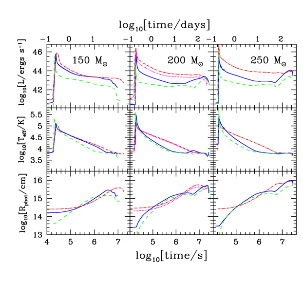
Figure 1.— Luminosities (top row), effective temperatures (center row), and photospheric radii (bottom row) of PPSNe for ten different representative models. Each sets of panels are labeled by the total mass of the progenitor star, and models with weak (dashed), intermediate (solid) and strong (dot-dashed) convective overshoot are shown. Finally, the dotted lines in the central panels correspond to model 200-S2. See text and Table 1 for details.

This mixing has two major effects on the PPSN progenitor: first, it increases the opacity and energy generation in the envelope, leading to a red-giant structure for the presupernova star, in which the radius increases by over an order of magnitude. Second, it decreases the mass of the He core, consequently leading to a smaller mass of ⁵⁶Ni being synthesized and a smaller explosion energy. The former effect increases the luminosity of the supernova, especially at early times, while the latter effect can weaken it. Just how much mixing occurs is uncertain from stellar modeling at the present, though it has been studied by several authors (e.g., Heger, Woosley & Waters 2000; Marigo et al. 2001). In the present paper we account for these uncertainties by employing different values of convective overshooting – whose presence is clear, but whose quantitative interaction with the burning is unknown.

A suite of representative models is chosen to address the expected range of presupernova models - from blue supergiant progenitors with little or no mixing to well-mixed red hypergiants, which can have pre-SN radii of 20 AU or more. These models are summarized in Table 1, in which the names refer to the mass of the progenitor star (in units of $\,{\rm M_{\odot}}$) and the weak (W), intermediate (I), or strong (S) level of of convective overshoot. Note, that in all cases the progenitor star is nonrotating, and all models employ the same procedure to mix ⁵⁶Ni into the envelope after the supernova shock.

The KEPLER code can be used to compute approximate light curves and has been validated both against much more complex and realistic codes such as EDDINGTON and observations of a prototypical Type II-P supernova, SN 1969L (Weaver and Woosley 1980; Eastman et al 1994). Its deficiency is that it is a single temperature code using flux-limited radiative diffusion. It functions very well, however, in situations where the light curve is recombination dominated (as on the plateau of Type II-P supernovae), in the radioactive peaks of Type I supernova, and in the tails of Type II-P supernovae. Gamma-deposition has been calibrated against a Monte Carlo code (Pinto and Woosley 1988) and the code was successfully used to predict the behavior of SN 1987A (Woosley, Pinto, & Ensman 1988), though mixing was later added as an essential ingredient. Because thermal equilibrium and black body spectra are assumed, the bolometric luminosity is known much better than the color photometry. Thus B and V magnitudes should be approximately correct, but U magnitudes are much more uncertain.

The resulting luminosities, effective temperatures, photospheric radii are shown in Figure 1. As the shock moves toward the low-density stellar surface, its energy is deposited into progressively smaller amounts of matter. This results in high velocities and temperatures when the shock reaches the stellar surface, causing a pulse of ultraviolet radiation with a characteristic timescale of a few minutes. This “breakout” phase is by far the most luminous and bluest phase of the PISN burst, but its very short duration makes it difficult to use in observational searches. In fact, the analog of this phase in conventional SN has so far only been indirectly detected in SN 1987A (Nayozhin 1994; Hamuy et al. 1988; Catchpole et al. 1988).

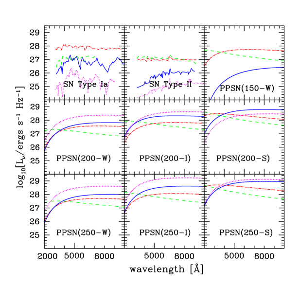
Figure 2.— Comparison of PPSNe spectra with those of Type Ia and Type II-P supernovae at 1 day (dashed), 10 day (dot-dashed), 100 days (solid), and 200 days (dotted) since explosion. The Type Ia spectra were taken from observations of SN 1994D, the Type II-P spectra were taken from observations of SN 1999em, and the PPSNe spectra were computed from black body models with $T_{\rm color}=T_{\rm eff}.$ While the overall shape of our simplified PPSNe spectra are similar to those of SNe Type Ia and Type II, their late-time evolution is markedly different, as seem most clearly in the 200 day curves.

Following breakout, the star expands with $R_{\rm phot}$ initially proportional to time. Though a small fraction of the outer mass may move much faster, the characteristic velocity of the photosphere during this phase is a modest $v=(2KE/M)^{1/2}\sim(10^{53}{\rm ergs}/200\,{\rm M_{\odot}})^{1/2}\sim 5000$ km/s, because of the very large mass participating in the explosion. During the expansion, the radiation-dominated ejecta cool adiabatically, with $T$ approximately proportional to $R^{-1},$ with an additional energy input from the decay of ⁵⁶Ni (if a significant mass was synthesized during the explosion) and hydrogen recombinations (when $T\sim 10^{4}$K). As the scale radius for this cooling is the radius of the progenitor, the temperatures and luminosities are substantially larger throughout this phase in the cases with the strongest mixing.

After $\sim 50$ days, the energy input from ⁵⁶Co decay becomes larger than the remaining thermal energy (the initial thermal energy deposited by the shock is mostly eaten away by the adiabatic expansion). At this time the energy deposited by ⁵⁶Co in deeper layers that were enriched in ⁵⁶Ni can diffuse out and these layers also become gradually more exposed as the outer parts of the supernova ejecta recombine and become optically thin. For stars that were compact to begin with, this can cause a delayed rise to the peak of the light curve. For stars with larger radii, the radioactivity just makes a bright tail following the long plateau in emission from the expanding envelope. Eventually, even the slow-moving inner layers recombine and there is no longer a well-defined photosphere. At this time the assumption of local thermodynamic equilibrium (LTE) breaks down, and more detailed radiative transfer calculations are required, which are beyond the scope of our modeling here. The SN is fainter and redder during this phase, however, and thus difficult to detect at cosmological distances in optical and near infrared (NIR) surveys.

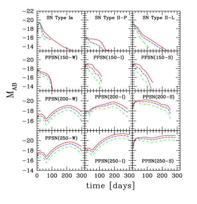
Figure 3.— Comparison of light curves of a SN Type Ia, a SN Type II-P, a bright SN Type II-L, and PPSNe models with varying progenitor masses. In all cases the solid lines are absolute V-band AB magnitudes, the dot-dashed lines are the absolute B-band AB magnitudes, and the dashed lines are the absolute U-band AB magnitudes.

3. Spectral Properties and Lightcurves

From the luminosities and effective temperatures in Figure 1, we calculated approximate PPSNe spectra, assuming a black body distribution with the color temperature equal to the effective temperature, that is the specific luminosity

$$L_{\nu}(t)=L(t)\frac{15x^{3}}{\nu_{0}\pi^{4}(e^{x}-1)},$$ (1)

where $x\equiv\nu/\nu_{0}$ and $\nu_{0}=2.1\times 10^{14}\,T_{\rm 4,eff}$ Hz, with $T_{\rm 4,eff}\equiv T_{\rm eff}/10^{4}$ K. Recall that the peak frequency in this case occurs at $5.9\times 10^{14}\,T_{\rm 4,eff}$ Hz, which corresponds to a wavelength of $5100\,T_{\rm 4,eff}^{-1}$ Å. The resulting spectra are plotted at representative times of 1, 10, 100, and 200 days in Figure 2, in which we also include comparison spectra from observations of Type Ia and Type II (core collapse) SNe. In particular, the Type Ia curves were taken from observations of SN 1994D by Patat et al. (1996) and Filippenko (1997) as compiled by Filippenko (1999), at 1, 10 and 128 days, and 233 days since explosion (assumed to be 13 days before B-max) normalized to Patat et al. (1996) and Cappelaro et al. (1997) V-band light curves at 1, 10, 100, and 200 days, with an assumed distance of 13.7 Mpc (see also Richmond et al. 1995). The Type II curves, on the other hand, were taken from spectra of the Type II-P SN 1999em by Elmhamdi et al. (2003) at 9, 10, 113, and 168 days since explosion, again normalized to their V-band light curves at 1, 10, 100, and 200 days, with an assumed distance of 7.8 Mpc.

The most striking feature from this comparison is that despite enormous kinetic energies of $\sim 50\times 10^{51}$ ergs, the peak optical luminosities of PPSNe are similar to those of other SNe, even falling below the Ia and II curves in many cases. This is because the higher ejecta mass produces a large optical depth and most of the internal energy of the gas is converted into kinetic energy by adiabatic expansion. Furthermore, the overall spectral shapes of the PPSN curves are not unlike those of more usual cases. In fact, pair-production supernovae spend most of their lives in the same temperature range as other SNe and therefore exhibit a similar range in colors throughout their evolution. Lastly, many of line features in the observed spectra would also be present in more detailed models of PPSNe. In particular, because of their hydrogen envelopes, PPSN spectra should contain hydrogen lines similar to those in Type-II SNe. Clearly, then, PPSNe will not be obviously distinguishable from their more usual counterparts “at first glance.”

A closer comparison between spectra, however, uncovers two key features that are uniquely characteristic to PPSNe. The first of these is a dramatically extended intrinsic decay time, which is especially noticeable in the models with the strongest enrichment of CNO in the envelope. This is due to the long adiabatic cooling times of supergiant progenitors, whose radii are $\sim 20$ AU, but whose expansion velocities are similar or even less than those of other SNe. Second, PPSNe are the only objects that show an extremely late rise at times $\geq 100$ days. This is due to energy released by the decay of ⁵⁶Co, which unlike in the Type Ia case, takes months to dominate over the internal energy imparted by the initial shock. In this case the feature is strongest in models with the least mixing and envelope enrichment during helium burning, as these have the largest helium cores and consequently the largest ⁵⁶Ni masses. Note, however, that neither of these features is generically present in all PPSNe, and both can be absent in smaller VMS that fail expand to large sizes through dredge-up and do not synthesize appreciable amounts of ⁵⁶Ni. In the 150-W case, for example, the luminosity decays monotonically on a relatively short time scale, producing spectra not dissimilar to the comparison Type II curves from SN 1999em. In fact this 150 $\,{\rm M_{\odot}}$ SN shares many similarities with its smaller-mass cousin: both are SNe from progenitors with radii $\sim 10^{13}$ cm and in both ⁵⁶Ni plays a negligible role.

In Figure 3 we examine the temporal evolution of PPSNe in more detail by plotting absolute AB light curves of our models at three representative wavelengths: 5500 Å, corresponding to the central wavelength of the V-band; 4400 Å, corresponding to the B-band; and 3650 Å, corresponding to the U-band. We focus on blue wavelengths as it is features in these bands that will be redshifted into the optical and NIR at cosmological distances. Again, for comparison, we also include in this figure observed light curves for SN Type Ia and Type II. In the Type Ia case the curves are again taken from observations of 1994D by Patat et al. (1996) and are supplemented at late times by data from Cappelaro et al. (1997). In the Type II case, we consider both Type II-P and Type II-L SNe. Our Type II-P curves are taken from observations of 1999em by Elmhamdi et al. (2003), and our Type II-L curves are taken from observations of the very bright supernova 1979C, as compiled in de Vaucouleurs et al. (1981) and Barbon et al. (1982), with an assumed distance of 17.2 Mpc (Freedman et al. 1994).

From this point of view, the characteristic features of PPSNe are even more striking, and the relation with progenitor structure is clear. Compact models with weak dredge-up are dominated by a late-time ⁵⁶Ni bump; extended hypergiant progenitor models with strong mixing show a significant blue early phase during the expansion followed by a longer, redder phase in which the luminosity is roughly constant for $\sim 200$ days; and intermediate models are a hybrid of the two. Finally, in cases such as the compact 150-W blue supergiant model, in which dredge-up does not occur and little ⁵⁶Ni is synthesized, both of these phases are absent, leaving an object remarkably reminiscent of more typical core collapse SNe, as exemplified by the Type II-P lightcurves. Similarly, models such as 150-I and 150-S which also synthesize very little ⁵⁶Ni, but are preceded by larger progenitors, are easily confused with bright Type II-L SNe, particularly at early times. In no case, however, do PPSNe look anything like SNe Type Ia. In particular none of the pair-production models display the long exponential decay seen in the Type Ia curves, and all PPSNe contain hydrogen lines, arising from their substantial envelopes.

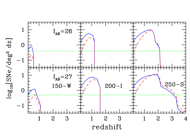
Figure 4.— Number of PPSNe per square degree per unit redshift above a given I-band magnitude, assuming 0.001 $\,{\rm M_{\odot}}$ yr^-1 Mpc^-3 (solid lines) or 1% of the observed star formation rate density (dashed lines). The $I_{AB}=26$ cut taken in the upper rows approximately corresponds to the magnitude limit of the Institute for Astronomy Deep Survey which covered 2.5 deg² (as shown by the dotted lines) from September 2001 to April 2002. The $I_{AB}=27$ limit in the bottom panel corresponds to that of the ongoing COSMOS survey, which will survey an area of 2 deg² (again indicated by the dotted lines). Note however, that the COSMOS survey itself is primarily focused on large-scale structure issues and will not be able to find PPSNe, as each pointing is visited only once.

4. Pair-Production Supernovae in Cosmological Surveys

From the models developed in §3, it is relatively straightforward to relate the star formation history of VMS to the resulting number of observable pair-production supernova. In this section and below we adopt cosmological parameters of $h=0.7$, $\Omega_{m}$ = 0.3, $\Omega_{\Lambda}$ = 0.7, and $\Omega_{b}=0.045$, where $h$ is the Hubble constant in units of 100 km s^-1 and $\Omega_{m}$, $\Omega_{\Lambda}$, and $\Omega_{b}$ are the total matter, vacuum, and bayonic densities in units of the critical density (e.g., Spergel et al. 2003).

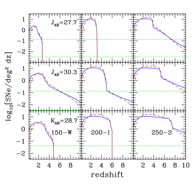
Figure 5.— Number of PPSNe per square degree per unit redshift above a fixed J or K-band magnitude, with limits appropriate for three possible realizations of the Joint Dark Energy Mission. Curves are as in Figure 4. Near infrared coverage allows for detection of PPSNe even after the lightcurves have been significantly redshifted. Top: The $J_{\rm AB}=27.7$ limit taken in these panels corresponds to that of a single scan in the planned deep-field SNAP survey, which would cover 7.5 deg² (indicated by the upper dotted lines). A similar magnitude limit with the same coverage would be obtained with 2 months of grism data from the Destiny mission. The full planned 700 deg² wide-field SNAP survey (lower dotted lines) also has the same limiting magnitude. Center: The $J_{\rm AB}=30.3$ limit taken in these panels is that of the deep-field SNAP survey, which would be able to place constraints on PPSNe out to $z\gtrsim 5.$ Bottom: Curves corresponding to the JEDI mission, whose redder photometry coverage allows for detections down to $K_{\rm AB}=28.7$ over 24 deg² with 2 months of data. This would place limits on PPSNe out to $z\sim 6$ and beyond.

Here we focus on three PPSN light curves, which bracket the range of possibilities: the faintest of all our models, 150-W, in which both significant dredge-up and ⁵⁶Ni production are absent; an intermediate model, 200-I, in which little dredge-up occurred, but 5.1 $\,{\rm M_{\odot}}$ of ⁵⁶Ni were formed; and the model with the brightest lightcurves, 250-S, in which substantial dredge-up leads to an enormous initial radius of over 20 A.U., and the production of 24.5 $\,{\rm M_{\odot}}$ of ⁵⁶Ni causes an extended late-time period of high luminosity. Accounting for redshifting, time dilation, and the appropriate luminosity and bandwidth factors, the specific flux for each of these models at a redshift $z$ observed at a wavelength $\lambda$ and a time $t$ after breakout (in the frame of the observer) is

$$F_{\nu}(\lambda,t,z)=\frac{L_{\nu}\left[\lambda(1+z)^{-1},t(1+z)^{-1}\right]}{4\pi r(z)^{2}(1+z)},$$ (2)

where $r(z)$ is the comoving distance associated with the supernova redshift. Note that this expression does not address the possibility of extinction by dust, which amounts to assuming that pristine regions remain dust-free thought the lifetime of the very massive PPSN progenitors stars. For any given PPSN model, we can then use eq. (2) to calculate $t(\lambda,F_{\nu}^{\rm min},z)$ the total time the observed flux at the wavelength $\lambda$ from a SN at the redshift $z$ is greater than the magnitude limit associated with the specific flux $F_{\nu}^{\rm min}.$ Finally, the total number of pair-production SNe shining at any given time with fluxes above $F_{\nu}^{\rm min}$, per square degree per unit redshift is given by the product of the volume element, the (time-dilated) PPSN rate density, and the time a given PPSN is visible, that is

$$\frac{dN_{\rm deg^{2}}}{dz}=[r(z)\,\sin(1{\rm deg})]^{2}\,\frac{dr}{dz}\frac{\rho^{\pm}(z)}{1+z}t(\lambda,F_{\nu}^{\rm min},z),$$ (3)

where the rate density $\rho^{\pm}(z)$ is the number of PPSNe per unit time per comoving volume as a function of redshift.

As $\rho^{\pm}(z)$ is completely unknown, we adopt here two simple models. In the first model, we assume that metal-free star formation occurs at a constant rate density, which we take to be $0.001\,\,{\rm M_{\odot}}\,{\rm yr}^{-1}\,{\rm Mpc}^{-3},$ independent of redshift. In the second case, we assume that at all redshifts metal-free stars form at 1% of the observed total star formation rate density, which we model as $\log_{10}[\rho^{\rm obs}_{\star}(z)/\,{\rm M_{\odot}}\,{\rm yr}^{-1}\,{\rm Mpc}^{-3}]=-2.1+3.9\,\log_{10}(1+z)-3.0\,[\log_{10}(1+z)]^{2},$ a simple fit to the most recent measurements (Giavalisco et al. 2004; Bouwens et al. 2004). Finally, for both star formation models we assume that 1 pair-production SN occurs per 1000 solar masses of metal free stars. This is consistent with typical estimates given in SSF03, in which $N^{\pm}$, defined as the number of PPSNe per solar mass of stars formed, was found to vary between $\sim 10^{-4}$ and $\sim 5\times 10^{-3}$ for a wide range of possible metal-free IMFs.

Note that while our two simple PPSN rate densities are chosen such that they can be easily rescaled by the reader, they are nevertheless consistent with the range of $z\gtrsim 1$ values predicted in more sophisticated models, as discussed in §5. Furthermore, the total amount of metals produced in our simple models is consistent with the element abundances observed in extremely metal-poor Galactic halo stars. Assuming a typical value of 200 $\,{\rm M_{\odot}}$ of metals ejected per PPSN and integrating down to $z=2.5$, one obtains values $\sim 6\times 10^{5}\,{\rm M_{\odot}}$ Mpc^-3 for both of our PPSN rate density models. This corresponds to a mass fraction of baryons that have been processed by VMS of $\sim 6\times 10^{-5}$, which is consistent with the $3-7\times 10^{-5}$ limits inferred by Oh et al. (2001) to explain the relative abundances in extremely metal-poor Galactic stars.

The resulting observed PPSNe counts for these models are given in Figure 4 for two limiting magnitudes. In the upper panels, we take a $I_{\rm AB}=26$ magnitude limit, appropriate for the Institute for Astronomy (IfA) Deep Survey (Barris et al. 2004), a ground-based survey that covered a total of 2.5 deg² from September 2001 to April 2002. As we are interested in rare objects, this type of survey is more constraining that a more detailed, smaller-area searches such as the Hubble Higher $z$ Supernova Search (Riess et al. 2004; Strolger et al. 2004).

From this figure we see that existing data sets, if properly analyzed, are easily able to place useful constraints on VMS formation at low redshifts. Given a typical PPSN model like 200-I for example, the already realized IfA survey can be used to place a constraint of $\lesssim 1\%$ of the total star formation rate density out to a redshift $\sim 1$. Similarly, extreme models such as 250-S can be probed out to redshifts $\sim 2$, all within the context of a recent SN search driven by completely different science goals. Note however that these limits are strongly dependent on significant mixing in the SN progenitor or the production of ⁵⁶Ni, and thus models such as 150-W remain largely unconstrained by the IfA survey.

In the bottom panels of Figure 4 we consider a limiting magnitude of $I_{\rm AB}=27$, appropriate for the COSMOS survey, an ongoing project that will cover 2 deg² using the Advanced Camera for Surveys on HST. Raising the limiting magnitude from $I_{\rm AB}=26$ to $I_{\rm AB}=27$ has the primary effect of extending the sensitivity out to slightly higher redshifts. This pushes the probed range from $z\lesssim 1$ to $z\lesssim 1.5$ in the 200-I case and from $z\lesssim 2$ to $z\lesssim 3$ in the 250-S case. Again this is all in the context of an ongoing survey. Even with this fainter limiting magnitude, however, low-luminosity PPSNe like 150-W are extremely difficult to find, and remain largely unconstrained.

This shortcoming is easily overcome by moving to NIR wavelengths. In Figure 5, we calculate the PPSN constraints that would be obtained from three possible realizations of the planned space-based Joint Dark Energy Mission (JDEM). In the upper and central panels of this plot we adopt two limiting $J$-band magnitudes, appropriate for the two surveys that would be carried out with the Supernova Acceleration Cosmology Probe (SNAP) realization of JDEM. In the upper panel we adopt a limit of $J_{\rm AB}=27.7$, corresponding to the depth of the planned (700 deg²) wide-field SNAP survey. With 2 months of data, the alternative Dark Energy Space Telescope (Destiny) realization of JDEM would cover 7.5 deg² of sky with spectroscopic observations down to a similar magnitude limit.

In these NIR surveys, ${dN_{\rm deg^{2}}}/{dz}$ is dramatically increased with respect to ground-based searches. This is due to the fact that for the majority of their lifetimes, the effective temperatures of PPSNe are just above the $\sim 10^{3.8}K$ recombination temperature of hydrogen, which corresponds to a peak black-body wavelength $\sim 8000$ Å. This means that for all but the lowest redshifts, the majority of the emitted light is shifted substantially redward of the I-band, which is centered at $9000$ Å. Thus moving to the J-band, which is centered at $12500$ Å, represents an exponential increase in the observed flux and allows for detections at significantly higher redshifts.

In the 200-I case, this results in number densities that are almost an order of magnitude higher than in the I-band. Combined with the larger area surveyed, this means that the wide-area SNAP survey could place constraints on this model that are roughly 300 times more stringent than those from the IfA survey, and these constraints would extend to $z\sim 4.$ Similarly tight limits can be placed on the 250-S model, but this time extending out to a redshift of 6. In fact, even very faint PPSNe like 150-W would be sensitively probed out to $z\sim 2.5.$ In the central panels we adopt a limit of $J_{\rm AB}=30$, corresponding to the depth of the planned (7.5 deg²) SNAP deep-field survey. In this case, both the 200-I and 250-S models would be well studied out to $z\gtrsim 5,$ and the 150-W model would be easily detectable out to $z\sim 4$ despite its overall low luminosity and relatively short lifetime.

Finally, in the lower panel, we consider an even redder 24 deg² survey with a limiting magnitude of $K_{\rm AB}=28.7,$ as appropriate for two months of observations from the Joint Efficient Dark-energy Investigation (JEDI) realization of JDEM. As the $K$ band is centered at $22000$ Å, such observations naturally push to even higher redshifts. Thus while reaching a limiting AB magnitude only slightly higher than the $700$ deg² SNAP survey, such a 24 deg² is able to place the most stringent of any of the surveys considered: constraining the 150-W model out to $z\sim 4$ and the more luminous models to $z\sim 6$ and beyond.

5. The Environments of Pair-Production Supernovae

As cosmological enrichment is essentially a local process, certain environments are naturally more favorable for metal-free star formation. In SSF03, we showed that the transition from metal-free to Population II stars was heavily dependent on the efficiency with which metals where mixed into the intergalactic medium. This efficiency depended in turn on the energy input into galactic outflows powered by PPSNe, which was parameterized by the “energy input per unit primordial gas mass” ${\cal E}_{\rm g}^{III}$, defined as the product of the fraction of gas in each primordial object that is converted into stars ($f_{\star}^{III}$), the number of PPSNe per unit mass of metal-free stars formed (${\cal N}^{\pm}$), the average kinetic energy per pair-production supernova (${\cal E}_{\rm kin}$), and the fraction of the total kinetic energy channeled into the resulting galaxy outflow ($f_{\rm wind})$.

Incorporating such outflows into a detailed analytical model of structure formation leads to the approximate relation that, by mass, the fraction of the total star formation in metal-free stars at $z=4$ is

$$F_{\star}^{III}(z=4)\sim 10^{-5}({\cal E}_{\rm g}^{III})^{-1},$$ (4)

where, as above, ${\cal E}^{\pm}$ is in units of $10^{51}$ ergs per $\,{\rm M_{\odot}}$ of gas (see Figure 3 of SSF03 for details). Extrapolating the results in SSF03 to $z=0$ gives

$$F_{\star}^{III}(z=0)\sim 10^{-5.5}({\cal E}^{III}_{\rm g})^{-1}.$$ (5)

These fractions can be related to the underlying population of stars by adopting fiducial values of $f_{\star}^{III}=0.1$ for the star formation efficiency, which is consistent with the observed star formation rate density at intermediate and high redshifts (Scannapieco, Ferrara, & Madau 2002); $f_{w}=0.3$ for the wind efficiency, which is consistent with the dwarf galaxy outflow simulations of Mori, Ferrara, & Madau (2002); and $N^{\pm}=0.001$, for the number of PPSNe per unit solar mass of primordial stars formed, which is the value assumed in §4. This gives $F_{\star}^{III}$ values of $0.3({\cal E}_{\rm kin})^{-1}$ at $z=4$ and $0.1({\cal E}_{\rm kin})^{-1}$ at $z=0,$ respectively. Or, in other words, for typical energies of $30\times 10^{51}$ ergs per PPSNe, $\sim 1\%$ of the star formation at $z=4$ and $\sim 0.3\%$ of the star formation at $z=0$ by mass could be in metal-free.

In Figure 6 we show estimates of the number of SNe per deg² per dz per year over the wide range of models considered in SSF03, extrapolating to $z=0.$ In all cases we assume that 1 PPSN forms per 1000 solar masses of metal-free stars, and for comparison we show the simple low-redshift estimates taken in the previous section. While the values in these models are uncertain, they nevertheless

Fig. 6.— Number of PPSNe per square degree per unit redshift per year for a wide range of models. As in Figs. 4 and 5, the solid and dashed curves assume Pop III star formation rate densities of 0.001 $\,{\rm M_{\odot}}$ yr^-1 Mpc^-3 and 1 $\%$ of the observed star formation rate density, respectively. The shaded region covers the range of metal-free star formation rate density models considered in SSF03, with the weakest feedback model (${\cal E}^{III}_{\rm g}=10^{-4}$) defining the upper end, and the strongest feedback model (${\cal E}^{III}_{\rm g}=10^{-2.5}$) defining the lower end. An extrapolation of these star formation rate densities to $z=0$ leads to the crosshatched region. In all SSF03 models the highest rates occur at redshifts $\leq 10.$ Finally, the starred point is the $z=15$ estimate by Weinmann & Lilly (2005).

serve to illustrate two important points. First, even at the low redshifts probed by current surveys, the simple range of VMS formation rates considered in §4 lie well within the theoretically interesting range. Indeed for the weakest feedback cases several $z\sim 1$ PPSNe should have already been seen within the IfA Deep survey. Secondly, due to the decrease in $dr$/$dz$ as a function of redshift, as well as the time dilation effect, the peak of $dN_{\rm deg}/{dzdt}$ is not in the $z\gtrsim 10$ range targeted by the James Webb Space Telescope, but rather at more moderate redshifts. This means that the constraints obtained from JDEM-type surveys are likely to reach comparable limits to higher-redshift efforts. In fact, it is extremely unlikely that PPSNe will be found at higher redshifts without similar detections at $z\lesssim 6.$

Note that for the full range of models in Figure 6, metal-free star formation naturally occurs in the smallest galaxies, just large enough to overcome the thermal pressure of the ionized IGM, but small enough not to be clustered near areas of previous star formation (SSF03). In our adopted cosmology, for an IGM temperature of $2\times 10^{4}$, the minimum virial mass is $8.4\times 10^{9}(1+z)^{-3/2}\,{\rm M_{\odot}}$ with a corresponding gas mass of $1.4\times 10^{9}(1+z)^{-3/2}\,{\rm M_{\odot}}.$ This means the total stellar mass of primordial objects is likely to be around $M_{\star}\sim 10^{8}\,{\rm M_{\odot}}(1+z)^{-3/2}$, many orders of magnitude below $L_{\star}$ galaxies. Thus in general blank-field surveys should be the best method for searching for PPSNe, as catalogs of likely host galaxies would be extremely difficult to construct.

Nevertheless, as VMS shine so brightly, a direct search for primordial host galaxies is not a hopeless endeavor. In particularly the lack of dust in these objects and the large number of ionizing photons from massive metal-free stars leads naturally to a greatly enhanced Lyman alpha luminosity. Following SSF03 this can be estimated as

$$L_{\alpha}=c_{L}(1-f_{\rm esc})Q(H)M_{\star},$$ (6)

where $c_{L}\equiv 1.04\times 10^{-11}$ ergs, $f_{\rm esc}$ is the escape fraction of ionizing photons from the galaxy, which is likely to be $\lesssim 0.2$ (see Ciardi, Bianchi, & Ferrara 2002 and references therein), and the ionizing photon rate $Q(H)$ can be estimated as $\approx 10^{48}$ s^-1 $\,{\rm M_{\odot}}^{-1}$ (Schaerer 2002). This gives a value of $L_{\alpha}\sim 10^{45}(1+z)^{-3/2}{\rm ergs\,s}^{-1}$ which, if observed in a typical $~{}1000$ Å  wide broad band corresponds to an absolute AB mag $\sim-23+3.8\log(1+z),$ much brighter than the PPSNe themselves. However this flux would be spread out over many pixels and be more difficult to observe against the sky than the point-like PPSNe emission. For further details on the detectability of metal-free stars though Lyman-alpha observations, the reader is referred to SSF03.

Finally we note that the presence of pair-production supernovae is generic to stars that die within a given range of helium core masses (HW02), and does not directly depend on metallicity. However there are three important theoretical reasons that make metal-free stars the favored progenitors of PPSNe. First, as $H_{2}$ becomes an inefficient coolant below a typical density and temperature of $\sim 10^{4}$ cm^-3 and $\sim 100$ K, fragmentation to masses smaller than $\sim 10^{3}\,{\rm M_{\odot}}$ is highly suppressed in gas of primordial composition (e.g., Abel, Bryan, & Norman 2002). Secondly, metal-rich VMS are prone to opacity-driven radial pulsations, which are suppressed in stars with metallicities below $\sim 10^{-3}Z_{\odot}$ (Baraffe, Heger, & Woosley 2001). Lastly, the lack of metals greatly reduces the line-driven wind mass loss, which is predicted to decline with metallicity as $Z^{1/2}$ or faster (Kudritzki 2000; Vink et al. 2001; Kudritzki 2002).

From an observational point of view, Figer (2005) carried out a detailed study of the IMF in the Arches cluster, which is large ($M_{\star}>10^{4}\,{\rm M_{\odot}}$), young ($\tau$ = 2.0 - 2.5 Myrs), and at a well-determined distance, making it ideal for such studies. No stars more massive than 130 $\,{\rm M_{\odot}}$ were found in this $Z\sim Z_{\odot}$ cluster, although more than 18 were expected. A similar $\sim 150\,{\rm M_{\odot}}$ limit was found in the lower metallicity cluster R136 in the Large Magellanic Cloud (Weidener & Kroupa 2003), and while mass estimates of a few stars exceed this limit, these values are quite uncertain. The Pistol star, for example, may in fact be a tight binary or have recently experienced a merger with another star (Figer & Kim 2002).

Intriguingly, the Arches cluster not only exhibits a cutoff at the highest masses but a flattened IMF above 50 $\,{\rm M_{\odot}}$ ($\Gamma=-0.9$ rather than the $-1.35$ Salpeter slope). Could some of these stars have been quickly whittled down from larger-mass progenitors? The answer is unclear. What is clear, however, is that there is little observational or theoretical evidence that the progenitors of PPSNe might be found in enriched environments.

6. Summary

Astronomers naturally associate metal-free star formation with extremely high redshifts. While the early universe contained no elements heavier than lithium, today stellar nucleosynthetic products are found in all measured Galactic halo stars, all nearby galaxies, and even in the low-density IGM. Yet it would be a mistake to conclude that such observations exclude metal-free star formation at moderate redshifts. Metal-enrichment is an intrinsically local process that proceeds over an extended redshift range, and at each redshift, the pockets of metal-free star formation are naturally confined to the lowest-mass galaxies, which are small enough not to be clustered near areas of previous star formation. As such faint galaxies are difficult to detect and even more difficult to confirm as metal-free, the hosts of PPSNe could easily be lurking at the limits of present-day galaxy surveys.

Using the implicit hydrodynamical code KEPLER we have constructed a suite of lightcurves that address the theoretical uncertainties involved in modeling PPSNe. Here the most important factors are the mass of the progenitor star and the efficiency of dredge-up of carbon from the core into the envelope. In general, increasing the mass leads to greater ⁵⁶Ni production, which boots the late time SN luminosity. Mixing, on the other hand, has two major effects: it increases the opacity in the envelope, leading to a red giant phase that increases the early-time SN luminosity; and it decreases the mass of the He core, consequently leading to a somewhat smaller mass of ⁵⁶Ni being synthesized. Despite these uncertainties, PPSNe in general can be characterized by three key features: (1) peak magnitudes that are brighter than Type II SNe and comparable or slightly brighter than typical SNe Type Ia; (2) very long decay times $\sim 1$ year, which result from the large initial radii and large masses of material involved in the explosion; and (3) the presence of hydrogen lines, which are caused by the outer envelope. Note, however, only this last feature is present in all cases, and in fact, the lowest mass PPSN models we constructed have lightcurves that are remarkably similar to those of SN Type II.

Accounting for redshifting, time dilation, and appropriate luminosity factors we used these lightcurves to relate the overall very massive star formation rate density to the number of PPSNe detectable in current and planned supernova searches. Here the long lifetimes help to keep a substantial number of PPSNe visible at any given time, meaning that ongoing SN searches should be able to limit the contribution of VMS to $\lower 2.15277pt\hbox{$\;\buildrel<\over{\sim}\;$}1\,$% of the total star formation rate density out to a redshift of 2, unless both mixing and ⁵⁶Ni production are absent for all PPSNe. Such constraints already place meaningful limits on the cosmological propagation of metals.

The impact of future NIR searches is even more promising, as the majority of the PPSN light is emitted at restframe wavelengths longward of $\sim 8000$ Å. Thus planned NIR satellite missions such as JDEM would be over two orders of magnitudes more sensitive to PPSNe than present optical surveys, and able to probe redshifts beyond $z\approx 6$. In this case, even the dimmest PPSNe would be detectable out to $z\approx 4$.

Although the peak of the metal-free star formation density almost certainly occurred at extremely early times, there is much to be learned from PPSN searches at more moderate redshifts. In fact, due to volume and time-dilation effects, the peak in the number of PPSNe per deg² per d$z$ per year is likely to lie well below $z=10.$ Furthermore, the data sets necessary for such analyses are already being planned for and collected. While the properties PPSNe are diverse, a singular conclusion can be drawn from our modeling. Searches for pair-production SNe at $z\lesssim 6$ will dramatically increase our understanding of the history of cosmic enrichment, the nature of metal-free stars, and the evolution of gaseous matter in the universe.

References

- (1)
- (2) Abel, T., Bryan, G., & Norman, M. 2000, ApJ, 540, 39
- (3) Abel, T., Bryan, G., & Norman, M. 2002, Science, 295, 93
- (4) Aracil, B., Petitjean, P., Pichon, C., & Bergeron, J. 2004, A&A, 419, 811
- (5) Baraffe, I., Heger, A., & Woosley, S. E. 2001, ApJ, 550, 890
- (6) Barbon, R., Ciatti, F., Rosino, L., Ortolani, S., & Rafanelli, P. 1982, A&A, 116, 43
- (7) Barkat, Z., Rakavy, G., & Sack, N. 1967, Phys. Rev. Lett., 18, 379
- (8) Barris, B. J., et al. 2004, ApJ, 602, 571
- (9) Blinnikov, S., Chugai, N., Lundqvist, P., Nadyozhin, D., Woosley, S., & Sorokina, E. 2003, in From Twilight to Highlight: The Physics of Supernovae, ed. W. Hillebrandt & B. Leibundgut (Berlin: Springer), 23
- (10) Bond, J. R., Arnett, W. D., & Carr, B. J. 1984, ApJ, 280, 825
- (11) Bouwens, R., et al. 2004, ApJ, 616, L79
- (12) Bromm, V., Ferrara, A., Coppi, P. S., & Larson, R. B. 2001, MNRAS, 328, 969
- (13) Bromm, V., & Loeb, A. 2003, Nature, 425, 812
- (14) Cappellaro, E., Mazzali, P. A., Benetti, S., Danziger, I. J., Turatto, M., Della Valle, M., & Patat, F. 1997, A&A, 328, 20
- (15) Catchpole, R. M., et al. 1988, MNRAS, 231, 75
- (16) Cayrel, R., et al. 2004, A&A, 416, 1117
- (17) Cen, R., Nagamine, K., & Ostriker, J. P. 2004, ApJ, submitted (astro-ph/0407143)
- (18) Ciardi, B., Bianchi, S., & Ferrara, A. 2002, MNRAS, 331, 463
- (19) Ciardi, B., Ferrara, A., & Abel, T. 2000, ApJ, 533, 594
- (20) Christlieb, N., et al. 2002, Nature, 419, 904
- (21) Dawson, S., et al. 2004, ApJ, 617, 707
- (22) de Vaucouleurs, G., de Vaucouleurs, A., Buta, R., Abels, H. D., & Hewitt, A. V. 1981, PASP, 93, 36
- (23) Dekel, A., & Rees, M. J. 1987, Nature 326, 455
- (24) Eastman, R. G., Woosley, S. E., Weaver, T. A., & Pinto, P. A. 1994, ApJ, 430, 300
- (25) Eastman, R. G., Woosley, S. E., Weaver, T. A., & Pinto, P. A. 1993, Bull. Am. Astron. Soc. 25, 836.
- (26) Elmhandi, A., et al. 2003, MNRAS, 338, 939
- (27) Figer, D. F. 2005, Nature, 434, 192
- (28) Figer, D. F., & Kim, S. S. 2002, in “Stellar Collisions, Mergers and their Consequences” ASP Series 263, ed. M. Shara
- (29) Filippenko, A. V. 1997, in “Thermonuclear Supernovae,” Girona, Spain, eds. P. Ruiz-Lauent, R. canal, & J. Isern
- (30) Filippenko, A. V. 1999, ARA&A, 35, 309
- (31) Freedman, W., et al. 1994, Nature, 371, 757
- (32) Fryer, C., L., Woosley, S. E., & Heger, A. 2001, ApJ, 550, 372
- (33) Fujita, A., Mac Low M.-M., Ferrara, A., & Meiksin, A. 2004, ApJ, 613, 159
- (34) Giavalisco, M. 2004, ApJ, 600, L103
- (35) Glover, S. C. O., & Brand, P. W. J. L. 2001, MNRAS, 321, 385
- (36) Haiman, Z., Rees, M. J., & Loeb, A. 1996, ApJ, 467, 522
- (37) Haiman, Z., Rees, M. J., & Loeb A., 1997, ApJ, 476, 458
- (38) Hamuy, M., Suntzeff, N. B., Gonzalez, R., & Martin, G. 1988, AJ, 95, 63
- (39) Heger, A., Woosley, S. E., & Waters, R. 2000, in “The First Stars,” Proc. MPA/ESO Workshop, p 121
- (40) Heger, A. & Woosley, S. E. 2002, ApJ, 567, 532 (HW02)
- (41) Heger, A., Woosley, S. E., Baraffe, I., & Abel, T. 2002, in “Lighthouses of the Universe: The Most Luminous Celestial Objects and Their Use for Cosmology,” Proc. of the MPA/ESO, p. 369 (astro-ph/0112059)
- (42) Heger, A., Fryer, C. L., Woosley, S. E., Langer, N., & Hartmann, D. H. 2003, ApJ, 591, 288
- (43) Herzig, K. et al. 1990, A&A, 233, 462
- (44) Kudritzki, R. 2000, The First Stars. Proceedings of the MPA/ESO Workshop held at Garching, Germany, 4-6 August 1999. Achim Weiss, Tom G. Abel, Vanessa Hill (eds.). Springer, p.127, 127
- (45) Kudritzki, R. P. 2002, ApJ, 577, 389
- (46) Machack, M . E., Bryan, G. L., & Abel, T. 2003, MNRAS, 338, 273
- (47) Mackey, J., Bromm, V., & Hernquist, L. 2003, ApJ, 586, 1
- (48) Marigo, P., Girardi, L., Chiosi, C., & Wood, P. R. 2001, A&A, 371, 152
- (49) Mori, M., Ferrara, A., & Madau, P. 2002, ApJ, 571, 40
- (50) Nakamura, F., & Umemura, M. 1999, ApJ, 515, 239
- (51) Nayozhin, D. K. 1994, in “Supernovae, Les Houches, Session LIV.” eds. S. A. Bludman, R. Mochkovitch, and J. Zinn-Justin (Elsevier Sci, Amsterdam), 571
- (52) Ober, W. W., El Eid, M. F., & Fricke, K. J. 1983, A&A, 119, 61
- (53) Oh, S. P. 2001, ApJ, 553, 25
- (54) Oh, S. P., & Haiman, Z. 2002, ApJ, 569, 558
- (55) Oh, S. P., Nollett, K. M., Madau, P., & Wasserburg, G. J. 2001, ApJ, 562, 1
- (56) O’Shea, Abel, T., Whalen, D. & Norman, M . L. 2005, ApJ, in press (astro-ph/0503330)
- (57) Patat, F., Benetti, S., Cappellaro, E., Danziger, I. J, Della Valle, M, Mazzali, P. A., & Turatto, M. 1996, MNRAS, 278, 111
- (58) Pettini, M., Madau, P., Bolte, M., Prochaska, J. X., Ellison, S., & Fan, X. 2003, ApJ, 594, 695
- (59) Pinto, P. A., & Woosley, S. E. 1988, ApJ, 329, 820
- (60) Renzini A. 1997, ApJ, 488,35
- (61) Richmond, M. W., Treffers, R. R., Filippenko, A. V., Van Dyk, S. D., Pail, Y., & Peng, C. 1995, AJ, 109 , 2121
- (62) Riess, A. G., et al. 2004, ApJ, 607, 665
- (63) Ripamonti, E., Haardt, F., Ferrara, A., & Colpi, M. 2002, MNRAS, 334, 401
- (64) Ryan, S. G., Norris, J. E., & Beers, T. C. 1996, ApJ, 471, 254
- (65) Scannapieco, E., Ferrara, A., & Madau, P. 2002, ApJ, 574, 590
- (66) Scannapieco, E., Schneider, R., & Ferrara, A. 2003, ApJ, 589, 35 (SSF03)
- (67) Schaerer, D. 2002, A&A, 382, 28
- (68) Schaye, J., Aguirre, A., Kim T.-S., Theuns, T., Rauch, M., & Sargent, W. L. W. 2003, ApJ, 596, 768
- (69) Schneider, R., Ferrara, A., Natarajan, P., & Omukai, K. 2002, ApJ, 571, 30
- (70) Searle, L. C., & Sargent, W. L. W. 1972, ApJ, 173, 25
- (71) Songaila, A. 2001, ApJ, 561, L153
- (72) Spergel, D. N., et al. 2003, ApJS, 14, 175
- (73) Strolger, L.-G., et al. 2004, ApJ, 613, 200
- (74) Tan, J. C., & McKee, C. F. 2004, ApJ, 603, 383
- (75) Theuns, T., Viel, M., Kay, S., Schaye, J., Carswell, R. F., & Tzanavaris, P. 2002, ApJ, 578, L5
- (76) Vink, J. S., de Koter, A., & Lamers, H. J. G. L. M. 2001, A&A, 369, 574
- (77) Weaver, T. A., Zimmerman, G. B., & Woosley, S. E. 1978, ApJ, 225,1021
- (78) Weaver, T. A., & Woosley, S. E. 1980, Ninth Texas Symposium on Relativistic Astrophysics, 335
- (79) Weidner, C., & Kroupa, P. 2003, MNRAS, 348, 187
- (80) Weinmann, S. N., & Lilly 2005, S. ApJ, 624, 526
- (81) Wise, J. H., Abel, T. 2005, ApJ, in press (astro-ph/0411558)
- (82) Woosley, S. E., Pinto, P. A., & Ensman, L. 1988, ApJ, 324, 466
- (83) Woosley, S. E., & Weaver, T. A. 1982, NATO ASIC Proc. 90: Supernovae: A Survey of Current Research, 79
- (84) Yoshida, N., Abel, T.,Hernquist, L., & Sugiyama, N 2003, ApJ, 593, 645