The Spherical Accretion Shock Instability in the Linear Regime

Abstract

We use time-dependent, axisymmetric, hydrodynamic simulations to study the linear stability of the stalled, spherical accretion shock that arises in the post-bounce phase of core-collapse supernovae. We show that this accretion shock is stable to radial modes, with decay rates and oscillation frequencies in close agreement with the linear stability analysis of Houck and Chevalier. For non-spherical perturbations we find that the $l=1$ mode is always unstable for parameters appropriate to core-collapse supernovae. We also find that the $l=2$ mode is unstable, but typically has a growth rate smaller than that for $l=1$. Furthermore, the $l=1$ mode is the only mode found to transition into a nonlinear stage in our simulations. This result provides a possible explanation for the dominance of an $l=1$ ’sloshing’ mode seen in many two-dimensional simulations of core-collapse supernovae.

1 Introduction

The modern paradigm for core-collapse supernovae includes a critical phase between stellar core bounce and explosion that is characterized by a stalled accretion shock, during which time neutrino heating is believed to reenergize, or at least play a critical role in reenergizing, the stalled shock [(Burrows et al., 1995; Mezzacappa et al., 1998; Rampp & Janka, 2000; Liebendoerfer et al., 2001; Buras et al., 2003; Fryer & Warren, 2004)]. (For a review, see Mezzacappa (2005).) This phase is expected to last of order a few hundred milliseconds.

The past decade has seen significant interest in the multidimensional dynamics of this post-bounce accretion phase. Most two-dimensional supernova simulations exhibit strong turbulent motions below the stalled accretion shock [(Herant et al., 1992; Miller et al., 1993; Herant et al., 1994; Burrows et al., 1995; Mezzacappa et al., 1998; Buras et al., 2003; Fryer & Warren, 2004)]. In the past, this turbulent flow was attributed to convection driven by the intense neutrino flux emerging from the proto-neutron star at the center of the explosion.

However, Blondin et al. (2003, hereafter Paper I) showed that the stalled accretion shock itself may be dynamically unstable. By using steady-state accretion shock models constructed to reflect the conditions in the post-bounce stellar core during the neutrino heating phase (as was shown in Paper I) but characterized by flat or positive entropy gradients, and as such convectively stable, Blondin et al. (2003) were able to isolate the dynamical behavior of the post-bounce accretion shock per se. They found that small nonspherical perturbations to the spherical accretion shock lead to rapid growth of turbulence behind the shock, as well as to rapid growth in the asymmetry of the initially spherical shock. This spherical accretion shock instability, or “SASI,” is dominated by low-order modes, and is independent of any convective instability.

Clearly, once the shock wave is distorted from spherical symmetry, the non-radial flow beneath it is no longer defined solely by neutrino-driven convection. The fluid flow beneath the shock is, at least initially, a complex superposition of flows generated by convection and by the SASI-distorted shock. Once the shock wave is distorted, it will deflect radially infalling material passing through it, leading to highly nonradial flow beneath it. With time, the fluid flow beneath the shock may in fact be determined by the SASI and not by convection. Instabilities such as neutrino-driven convection may be important only at early times in aiding the neutrino heating (Herant et al., 1994; Burrows et al., 1995; Mezzacappa et al., 1998; Buras et al., 2003; Fryer & Warren, 2004) and in setting the shock standoff radius while the explosion is initiated. The standoff radius will in turn determine the time scale over which the SASI may develop.

Janka (2001) provides a qualitative description of this post-bounce accretion phase in terms of a simple hydrodynamic model, with the intent of providing an analytic model that can be used to investigate the conditions necessary for a successful supernova shock. In this picture the post-bounce phase is described by a standing accretion shock with outer core material raining down on the shock at roughly half the free-fall velocity. After traversing the shock, this gas decelerates and gradually settles onto the surface of the nascent neutron star. The pressure of this post-shock gas is dominated by electron-positron pairs and radiation, and as such can be modeled as a $\gamma=4/3$ gas. The approximation of an hydrostatic atmosphere immediately below the accretion shock then yields the result that the gas density increases as $r^{-3}$ and the gas pressure increases as $r^{-4}$ with decreasing radius behind the shock. Deeper within this settling region, the gas pressure becomes dominated by non-relativistic nucleons and the temperature becomes roughly constant due to neutrino emission. The flow below this transition radius can thus be approximated by an isothermal hydrostatic atmosphere. The steady nature of this accretion shock and post-shock settling solution is maintained by a balance between fresh matter accreting through the standing shock, and dense matter cooling via neutrinos and condensing onto the surface of the nascent neutron star (Chevalier, 1989; Janka, 2001).

This model of core-collapse supernovae described by Janka (2001) is similar to the analytic models presented by Houck & Chevalier (1992, hereafter HC) to investigate spherical accretion flows onto compact objects. These latter models assume the flow can be treated as an ideal gas with a single effective adiabatic index, $\gamma$, and a cooling function with a prescribed power-law dependence on the local density and temperature of the gas. Using a linear stability analysis HC showed that extended shocks (where the shock radius, $R_{s}$, is much larger than the stellar radius, $r_{*}$) are unstable to radial oscillations. For $\gamma=4/3$ this critical radius was $R_{s}\sim 20r_{*}$ or larger, depending on the cooling parameters. This is larger than is expected in the post-bounce accretion phase of core-collapse supernovae, suggesting that the stalled supernova shock is stable to radial perturbations. HC examined one case with $\gamma=5/3$ for the stability of nonradial modes, and found that only the lowest order nonradial mode ($l=1$ in terms of Legendre polynomials) was unstable. However, the growth rate for the $l=1$ mode was slower than that for the radial ($l=0$) mode. They did not present results for nonradial modes for any case with $\gamma=4/3$.

The focus of this paper is to develop a deeper understanding of the SASI by focusing on its development in the linear regime and in the transition from linear to nonlinear behavior and to supplant through such analyses the numerical findings in Paper I. In so doing, ties to and extensions of the linear stability analyses of HC can be made as well, which in part serve to validate the findings made with our multidimensional hydrodynamics code.

We begin by describing the model in Section 2 and the numerical method with which we evolve the time-dependent flow in Section 3. The results from one-dimensional models are reported in Section 4, along with the corresponding results from HC. In Section 5 we present two-dimensional simulations, quantifying the SASI growth rate as a function of the Legendre wave number, $l$, and illustrating the physical origin of the $l=1$ instability.

2 Spherical Accretion Shock

We begin with the model of the post-bounce accretion shock and “settling” flow beneath it presented in Paper I. As we now discuss, this model is a limiting case of the model presented in Janka (2001) and is defined following the prescription outlined in the earlier work by HC. In our model, we assume we have an ideal gas equation of state, a cooling function, and a hard reflecting boundary at the surface of the accreting compact object. We make the additional assumption that the gas in the postshock region is radiation-dominated—that is, that we have a single adiabatic index. This is appropriate for conditions in the postbounce stellar core at a time when explosion is initiated, during which time we expect an extended heating region overlaying a thin cooling region above the proto-neutron star surface. Of course, the equilibrium radius of the accretion shock is determined by the magnitude of the cooling in this cooling layer: stronger cooling leads to a shock radius closer to the inner reflecting boundary, while weaker cooling results in a shock with a large stand-off distance from the accreting object. While one could include a neutrino heating term in such a model (Burrows & Goshy, 1993), this would possibly introduce convection in the dynamics, complicating the analysis. Because our goal is to separate the effects of shock-driven turbulence from thermally-driven convection, we do not include any heating term in our models.

The time-evolution of the flow is given by the Euler equations for an ideal gas described by a velocity, $\bf u$, a mass density, $\rho$, and an isotropic thermal pressure, $p$:

$$\partial_{t}\rho+\nabla\cdot\rho{\bf u}=0$$ (1)

$$\partial_{t}\rho{\bf u}+\nabla\cdot\rho{\bf uu}+\nabla p=-\rho{GM}/{r^{2}}$$ (2)

$$\partial_{t}\rho{\cal E}+\nabla\cdot(\rho{\cal E}{\bf u}+p{\bf u})=-{\cal L}$$ (3)

where the total energy per gram is given by ${\cal E}=\frac{1}{2}{\bf u}^{2}+e-GM/r$, the internal energy, $e$, is given by the equation of state: $\rho e=p/(\gamma-1)$, and $M$ is the mass of the accreting star.

Following HC, the cooling term is parameterized by two power-law exponents:

$${\cal L}=A\rho^{\beta-\alpha}p^{\alpha}.$$ (4)

Using the parameterization of effective neutrino cooling provided by Janka (2001), with $\dot{E}\propto\rho T^{6}$, and assuming $P\propto T^{4}$, we arrive at values of $\alpha=3/2$ and $\beta=5/2$ for our model.

Following Paper I, we normalize the problem such that $GM=0.5$, $\dot{M}=4\pi$, and the equilibrium accretion shock is at $R_{s}=1$. Note that this results in the same normalization for density, velocity, and pressure as used in HC. Assuming free-fall velocity just above the accretion shock, the immediate post-shock values are then given by

$$u_{s}=\frac{\gamma-1}{\gamma+1},\rho_{s}=\frac{\gamma+1}{\gamma-1},p_{s}=\frac{2}{\gamma+1}.$$ (5)

The equilibrium solutions are obtained by integrating the Euler equations inward from the shock front until $u=0$, corresponding to the surface of the accreting star. These equilibrium solutions are shown in Figure 1 for three different values of $r_{*}$, and hence three different stellar radii relative to the normalized shock radius.

Figure 1: Equilibrium solutions for the spherical accretion shock model of a core-collapse supernova are shown for different values of the radius of the proto-neutron star ($r_{*}$ = 0.04, 0.2, 0.5) relative to the shock radius. The velocity and entropy are integrated inwards from the accretion shock at $R_{s}=1$ to the stellar surface at $r_{*}$.

The entropy profiles show in Figure 1 illustrate the regime of strong neutrino cooling in this supernova model. In the absence of cooling the flow would remain isentropic, thus the drop in entropy seen in Figure 1 reflects the local efficiency of cooling, which is predominantly confined to a thin layer at the surface of the accreting star. Furthermore, as the stellar radius recedes from the shock front (a more extended shock region), this cooling layer becomes progressively thinner.

There are two characteristics of our models that warrant further discussion, particularly as they compare to past supernova models: (1) The mass accretion rate through the shock is assumed to be constant. In reality, the accretion rate decreases with time owing to the decreasing density and velocity in the preshock gas. Therefore, the results we present here would be enhanced if the drop-off in mass accretion rate were included. (2) We assume a high Mach number for the shock (anything $\sim 3$ or larger would be sufficiently large to be consistent with our models). This assumption is consistent with the profiles found in supernova models (e.g., see Mezzacappa et al. (2001)).

3 Numerical Model

As described in Paper I in more detail, we use the time-dependent hydrodynamics code VH-1 (http://wonka.physics.ncsu.edu/pub/VH-1/) to study the dynamics of a spherical accretion shock in both one and two dimensions. A critical aspect of this numerical implementation is the use of dissipation to maintain a smooth flow in the absence of any perturbations (Paper I).

These models are described by four parameters, $\gamma$, $\alpha$, $\beta$, and $r_{*}$ (or $A$). Note that although the parameters $A$ and $r_{*}$ are equivalent, they are not related by a closed-form expression. We therefore numerically search for the value of $A$ that produces a steady shock at a radius of unity for a given inner reflecting boundary at a radius of $r_{*}$. This steady-state solution is then mapped onto a radial grid extending from $r_{*}$ to $2R_{s}$ to initialize the numerical simulations. The shock front is smoothed over two numerical zones to minimize spurious waves at the start of the simulation.

The numerical resolution required for an accurate solution depends on the parameters of the problem, namely the scale-height of the cooling region. We found appropriate resolutions empirically by evolving one-dimensional simulations at various resolutions and comparing the time-evolution of the shock radius. We used grids with 300 to 450 radial zones, including a small increase (never more than 1%) in the radial width of the zones to maximize resolution near $r_{*}$ where rapid cooling generates strong gradients. The two dimensional simulations use the same number of zones used in the radial direction to cover the polar angle (a limitation of the parallel algorithm used by VH-1) from $0$ to $\pi$, assuming axisymmetry about the polar axis. The fluid variables at the outer boundary are held fixed at values appropriate for highly supersonic free-fall at a constant mass accretion rate, consistent with the analytic standing accretion shock model. Reflecting boundary conditions were implemented at the inner boundary, $r_{*}$. For the two-dimensional simulations, reflecting boundary conditions were applied at the polar boundaries and the tangential velocity was initialized to zero everywhere in the computational domain.

4 Code Verification

The results of HC provide an opportunity to verify our numerical code on a time-dependent flow problem of direct relevance to core-collapse supernovae. Their linear stability analysis shows that spherical accretion shocks are unstable to growing oscillations in the shock radius (for the fundamental mode) if the shock is relatively extended.

To confirm this stability analysis and to verify our numerical code, we have run simulations matching the parameterization for post-supernova fallback used in HC. They considered the problem of fall back onto the nascent neutron star on the time scale of hours to days following the supernova explosion. In this case the gas is optically thick and radiation-dominated ($p\propto T^{4}$, $\gamma=4/3$, as in the present post-bounce model). Near the surface of the accreting neutron star, the gas is loosing energy through neutrino cooling with a negligible density dependence but a strong temperature dependence ($\dot{E}\propto T^{10}$). These properties are approximated in the present model by considering the parameter values $\alpha=\beta=2.5$ (Chevalier, 1989). We note that the fall-back solutions used by HC and the post-bounce solutions described in this paper are very similar.

Figure 2: The real and imaginary parts of the growth rate, $\omega$, as a function of the shock height, $R_{s}/r_{*}$ for the fall-back model. Results are shown for the linear stability analysis of HC (solid line) and for the 1D numerical simulations described in this paper (dashed line). Note that the values from HC have been transformed to the units used in this paper.

We perturb the equilibrium solutions by dropping an over-dense shell onto the shock, which compresses and pressurizes the shock region. The overpressure drives the shock back outwards, and in addition a strong pressure wave rebounds off the stellar surface and drives the accretion shock out even faster. This sets up an oscillation of the shock region on the sound crossing timescale. For parameters typical in core-collapse supernovae this oscillation is damped, as it was in the adiabatic models of Paper I. For very extended shocks this oscillation is overstable; for the fall-back case this critical radius is $r_{*}\approx 0.05$.

To extract a complex growth rate from these simulations we fit the simulation data for the shock radius, $R_{s}(t)$, to an analytic function of the form

$$R_{s}(t)=R_{0}+R_{1}e^{\omega_{r}t}\sin(\omega_{i}t+\delta).$$ (6)

Using least-squares fitting we obtain the real and imaginary parts of the growth rate, $\omega$. The results from several simulations of the fall-back model are shown in Figure 2, together with the linear growth rates derived by HC. There is only a limited range in $R_{s}/r_{*}$ where the linear analysis and the numerical simulations overlap, but within that overlap the agreement is remarkably good.

Simulations of very extended shocks ($r_{*}\ll R_{s}$) become computational expensive because of the large dynamic range in spatial coverage and the extremely short time scale. As $r_{*}$ becomes much smaller than $R_{s}$, the region of strong cooling (for $\gamma=4/3$) shrinks to a small fraction of $r_{*}$. This forces the use of a high resolution spatial grid near $r_{*}$, which in turn requires a large number of computational zones and a very small time step due to the Courant condition: $\Delta t<\Delta r/c_{s}$. As an extreme example, to simulate a model with $r_{*}=0.01$ required 200,000,000 timesteps.

These simulations do two important things: they confirm the linear stability analysis of HC, and they validate our time-dependent numerical model.

5 Linear Evolution of the SASI

We performed a series of two-dimensional axisymmetric simulations following the same procedure outlined above for one dimension, down to the same radial gridding for a given model. We experimented with a variety of ways to perturb the equilibrium solution with the goal of exciting a single mode (in terms of spherical harmonics) with as little power in other modes as possible. This goal was best achieved when using density enhancements in the preshock gas as had been used in 1D. These density variations were typically between 0.1% and 1%; large enough to excite the instability but small enough that the perturbations could grow in amplitude by more than an order of magnitude while still remaining small. This extended regime of linear growth facilitated an accurate measurement of the linear growth rate. As in Paper I, all of the two-dimensional simulations were unstable. Here we attempt to quantify the growth rate of this instability in the linear regime as a function of the wave number.

To track the importance of various modes affecting the stability of a spherical accretion shock, the evolution was tracked using Legendre polynomials. Again, after trying several methods, we found the best approach was to first integrate the amplitude in a given harmonic for a fixed radius,

$$G(r)=\int A(r,\theta)P_{l}(\cos\theta)d\cos\theta$$ (7)

and then integrate the power for that harmonic over radius:

$$Power=2\pi\int\left[G(r)\right]^{2}r^{2}dr$$ (8)

where $A(r,\theta)$ represents some local quantity affected by the perturbed flow, e.g., entropy or pressure, and $P_{l}$ is the Legendre polynomial of order $l$.

Figure 3: The growth of the SASI in a simulation with $r_{*}=0.2$ is quantified here by the power in the perturbed entropy for the $l=1$ mode (solid line). The best fit to this growth curve is shown as a dashed line. The SASI becomes nonlinear at a time around $t\approx 60$, as shown by the deviation of $\langle R_{s}\rangle$ from unity.

An example of the linear growth of the SASI is shown in Figure 3 for $r_{*}=0.2$. These simulations exhibit a well-defined regime of exponential growth spanning at least an order of magnitude in amplitude. The beginning of a simulation is typically marked by a complex pattern of waves, but given an appropriate initial perturbation, a single mode soon dominates the evolution. To provide guidance on the relevance of the linear regime, we also show the angle-averaged shock radius throughout the evolution. During the linear regime, when perturbations to the spherical accretion flow are small, we expect the shock to remain nearly stationary. Once the average shock radius begins to deviate substantially from unity, the SASI has entered the non-linear regime.

As in the analysis of the one-dimensional simulations, we can fit these growth curves from two-dimensional simulations with an exponentially growing sinusoid. In this case, we are fitting the power, not the radius:

$$F(t)=F_{1}e^{2\omega_{r}t}\sin^{2}(\omega_{i}t+\delta).$$ (9)

The fitted frequencies are shown in Figure 4 for four different values of $r_{*}$ (0.5, 0.3, 0.2, and 0.1). We did not attempt simulations for smaller values because they would have required an extremely long integration, and the results for the $r_{*}=0.1$ model were sufficiently noisy that we did not expect to be able to extract clean growth rates from more extended models. Note, however, that the growth rate of the $l=1$ mode appears to be decreasing for very extended shocks and that the $l=0$ mode becomes unstable for $r_{*}<.05$.

We do not consider values of $r_{*}$ larger than 0.5 because this would not be consistent with our fundamental starting assumption of having conditions near explosion and a postshock gas described by a single adiabatic index. Under such conditions, we would have a large heating region dominated by radiation and a thin cooling layer at its base. A larger value of $r_{*}$ would imply a larger cooling region and, generally, a postshock region composed of gases with different adiabatic indices.

Figure 4: The real and imaginary parts of the growth rate, $\omega$, as a function of the shock radius relative to the stellar radius, $R_{s}/r_{*}$ for three different axisymmetric modes, $l=0$, 1, and 2.

We could not isolate modes with values of $l>2$, nor could we adequately measure the growth of the $l=2$ mode in the most extended models with $r_{*}=0.1$. The results for the spherically symmetric mode ($l=0$) are taken from the one-dimensional simulations. As expected, the frequency of oscillation is a monotonically increasing function of the wavenumber. The growth rate, however, is not. In all cases we found that $l=1$ is the most unstable, and is always unstable.

Figure 5: The growth of the SASI in a simulation excited with the $l=2$ mode (dashed line) but dominated at late times by the $l=1$ mode (solid line). The SASI becomes nonlinear at a time around $t\approx 120$, once the $l=1$ mode becomes dominant.

At late times the evolution is always dominated by the $l=1$ mode. In fact, this is the only mode that we have observed to reach a nonlinear stage. We show in Figure 5 the growth of the different modes in a simulation for which we carefully excited the $l=2$ mode and not the $l=1$ mode. While the $l=2$ mode grows substantially over the course of a dozen oscillations, it stops growing before reaching the nonlinear stage. In contrast, the $l=1$ mode grows up out of the noise and becomes nonlinear at a time of about $t\approx 120$. We speculate that the linear growth of the $l=2$ mode stalls because power in that mode is lost to the rapidly growing $l=1$ mode. Note that the power in $l=1$ is very chaotic during this episode when the $l=2$ growth stalls. In fact, a comparison of Figures 3 and 5 shows that the overall growth rate for $l=1$ is steeper in this latter model than observed for a simulation with only an $l=1$ mode excited. While it might be possible for the $l=2$ mode to reach a nonlinear stage if the $l=1$ mode was completely suppressed, one would not expect such an artificial situation to happen in Nature.

To understand the physical origin of the SASI, we first note that the oscillation frequency of the SASI corresponds roughly to the time it takes a sound wave to cross the spherical accretion shock cavity. For the model with $r_{*}=0.2$, a sound wave travels from $R_{s}$ to $r_{*}$ in a time of 1.51. Neglecting the path around the stellar surface at $r_{*}$, a sound wave would travel back and forth across the spherical cavity in a characteristic time $\tau_{s}\approx 6$, giving an oscillation frequency of $\omega_{i}\approx 1$. Note that a more realistic path around the central star would give a longer travel time, both because of the longer path length and because the sound speed is slower at larger radii. Thus, one would expect a frequency somewhat smaller than unity, in agreement with the results shown in Figure 4. In contrast, the advection time for a parcel of gas to drift in from $R_{s}$ to $r_{*}$ is 14.3 for this same model. Therefore, any small perturbations in advected quantities (e.g., $u_{\theta}$, vorticity, entropy) are seen to drift inwards on a time scale much longer than the characteristic time scale of the SASI.

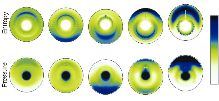
Figure 6: An example of the perturbed variables taken from the simulation excited with an $l=1$ mode. The entropy is shown in the top row and pressure in the bottom row. In each case blue represents positive deviations from equilibrium and white represents negative. Time evolves to the right over one period of oscillation; the first and last images represent the same phase. An mpeg animation of this evolution is available on line.

This difference between the propagation of sound waves and the slower drift of advected perturbations can be seen in Figure 6, where we show the time evolution of two flow quantities. In the case of entropy, which serves as a marker of fluid elements when the gas is adiabatic (which is the case all but near the accreting surface), the perturbations advect radially inward and fade away into the low-entropy gas of the cooling layer. These perturbations are generated at the shock and advect inwards with the accretion flow. As such, they have no means of directly influencing the accretion shock. Furthermore, there is no evidence of pressure perturbations at small radii that might represent acoustic waves originating from these flow perturbations as they advect inward—i.e., of a vortical–acoustic feedback. In contrast, the bottom row in Figure 6 shows something that resembles a standing wave pattern rather than features drifting radially inward with the flow. For example, the region of high pressure does not propagate across the equator of the shock, but rather fades in one hemisphere only to grow in the low pressure region in the opposite hemisphere. Based on these observations, we conclude that the SASI is the result of a growing standing pressure wave oscillating inside the cavity of the spherical accretion shock.

Figure 7: The effect of changing the shock position on the post-shock pressure profile is illustrated here with two different equilibrium solutions. The dashed line shows the immediate post-shock pressure as a function of shock location. Thus in each case the pressure begins on this line at the position of the shock and varies approximately as $r^{-4}$ inward. If the shock is displaced outward by a small amount, from a radius of 1.0 to a radius of 1.1, the pressure of the inflowing gas behind the perturbed shock will start off at a lower value, but it will be higher at each radius below 1.0 than it is for the inflowing gas behind the original equilibrium shock. This positive feedback drives the growth of the acoustic waves, creating the SASI.

The origin of the growth of this standing wave can be traced to the response of the post-shock pressure to changes in the shock radius. If the pressure in one hemisphere becomes slightly higher than equilibrium, it will push the spherical accretion shock outwards. Because the preshock ram pressure drops with increasing radius (as $r^{-2.5}$), shown by the dashed line in Figure 7, the outward shock displacement leads to a smaller pressure immediately behind the shock. However, given that the postshock pressure increases with decreasing radius as $r^{-4}$, the postshock pressure for the perturbed shock will be greater than the postshock pressure for the unperturbed shock at each radius below the radius of the original unperturbed shock. This is illustrated with the two cases shown in Figure 7. The postshock pressure immediately behind the shock for the perturbed shock at radius 1.1 is lower than the postshock pressure immediately behind the unperturbed shock at radius 1.0 given the decrease in the preshock ram pressure given by the dashed line. However, at each radius below 1.0 the postshock pressure for the perturbed shock is higher than the postshock pressure for the unperturbed shock.

There is an additional effect on the immediate post-shock pressure due to the change in shock velocity. As the shock is being pushed outward, the local shock velocity is larger than for a stationary shock at that radius, leading to a slightly higher post-shock pressure. Note that the change in pressure due to shock velocity is out of phase with respect to the change in pressure due to shock displacement, with the former peaking as the shock is moving outward, and the latter peaking at a phase $\pi/2$ later when the shock has reached its maximum extent. Nonetheless, both effects act to amplify the pressure variation of the standing wave. For the observed frequencies of the $l=1$ mode of the SASI, the effect of changing shock velocity is a few times smaller than the change in ram pressure due to shock displacement.

The linear phase of the SASI is characterized by a nearly spherical accretion shock and approximately radial post-shock flow. Once the amplitude of the standing pressure wave becomes large enough to significantly break the spherical symmetry of the accretion shock, the SASI enters the non-linear phase. In this phase the radially infalling gas above the shock strikes the shock surface at an oblique angle, generating strong, non-radial post-shock flow. This transition from the linear to non-linear phase is illustrated in Figure 8. The effect of a distorted shock on the post-shock flow is quite dramatic even for the relatively slight changes in shock position shown in the second frame of Figure 8. Although the accretion shock is nearly spherical in this frame, it is significantly displaced upward. As a result, the post-shock flow is no longer radial, and in some regions is almost entirely tangential to the radial direction. As a consequence of this non-radial flow, perturbations generated on one side of the shock can be advected across the interior and over to the other side of the accretion cavity. For example, the second frame in Figure 8 shows a shell of high-entropy gas (shown in blue) in the upper hemisphere being advected around the central star and toward the lower hemisphere.

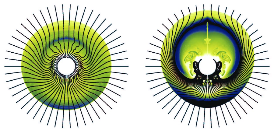
Figure 8: The transition from the linear to the non-linear regime is illustrated with these two images spanning one oscillation period. The color shows positive (blue) and negative (yellow/white) deviations to the equilibrium value of gas entropy, and the lines represent streamlines integrated along the instantaneous velocity field. The transition to the nonlinear regime is largely characterized by the transition from radial to nonradial flow. An mpeg animation of this transition is available on line.

6 Discussion and Conclusion

The linear stability analysis presented here has illuminated the underlying physical origin of the SASI instability first presented in Paper I. The SASI is not the result of a vortical–acoustic feedback (Foglizzo, 2002) seen in other contexts, as thought previously (Paper I). Rather, it is the result of a growing standing acoustic wave in the spherical cavity bounded below by the surface of the compact object and above by the accretion shock. This is our primary finding.

In addition, our techniques for exciting different modes in isolation, first defined in Paper I and refined here, and for defining and extracting the growth rate of these modes in the linear regime, have confirmed that the SASI is an $l=1$ instability, first proposed in Paper I. This result provides a possible explanation for the large-scale structure seen in recent two-dimensional supernova simulations performed on numerical grids covering a full $\pi$ in angle Janka et al. (2004). Our results clearly show that the $l=2$ mode is unstable, but we have not observed this mode becoming nonlinear. Rather, the amplitude of the $l=1$ mode always overtakes that of the $l=2$ mode during the linear regime. In the two-dimensional case considered here, it is apparent that, in the linear regime, power is transferred from the $l=2$ to the $l=1$ mode with time.

Under near explosive conditions at the onset of a core collapse supernova (large neutrino heating region, thin neutrino cooling region), our results strongly suggest the SASI will develop. Moreover, the SASI has been confirmed in a two-dimensional model by Janka et al. (2004) that included neutrino transport and suppressed neutrino-driven convection in order to isolate, as we have done here, postshock flow induced by the SASI versus postshock flow induced by convection. And the development of an obvious $l=1$ mode in the explosion of an 11 M_⊙ progenitor in a simulation performed by the same group on a 180 degree angular grid, without any such suppression, is strong evidence for the SASI in a complete model that attains explosive conditions Janka et al. (2004). Moreover, given that this very same model did not explode when a 90 degree grid was used Buras et al. (2003), one must consider that the SASI will play an important role in the explosion mechanism per se, as proposed in Blondin et al. (2003), not just in defining gross characteristics of the explosion.

Generally speaking, we have affirmed the discovery of the SASI in core collapse supernovae Paper I and supplanted our understanding of its origin and development. Relatively small-amplitude perturbations, whether they originate from inhomogeneities in the infalling gas, aspherical pressure waves from the interior region, or perturbations in the postshock velocity field, can excite perturbations in the standing accretion shock that lead to vigorous turbulence and large-amplitude variations in the shape and position of the shock front. In addition, we have confirmed the linear stability analysis of HC for spherically symmetric modes, providing a critical test of our numerical hydrodynamic algorithm in the context of core-collapse supernovae.

References

- Blondin et al. (2003) Blondin, J. M., Mezzacappa, A., & DeMarino, C. 2003, ApJ, 584, 971
- Buras et al. (2003) Buras, R., Rampp, M., Janka, H.-Th. & Kifonids, K. 2003, PhRvL, 90, 1101
- Burrows & Goshy (1993) Burrows, A. & Goshy, J. 1993, ApJ, 416, L75
- Burrows et al. (1995) Burrows, A., Hayes, J. & Fryxell, B. A.1995, ApJ, 450, 830
- Chevalier (1989) Chevalier, R. A. 1989, ApJ, 346, 847
- Foglizzo (2002) Foglizzo, T. 2002, A&A, 392, 353
- Fryer & Warren (2004) Fryer, C. L. & Warren, M. S. 2004, ApJ, 601, 391
- Herant et al. (1992) Herant, M., Benz, W. & Colgate, S. A. 1992, ApJ, 395, 642
- Herant et al. (1994) Herant, M., et al. 1994, ApJ, 435, 339
- Houck & Chevalier (1992) Houck, J. C. & Chevalier, R. A. 1992, ApJ, 395, 592
- Janka (2001) Janka, H.-T. 2001, A&A, 368, 527
- Janka et al. (2004) Janka, H.-T., Buras, R., Kitaura Joyanes F.S., Marek, A. & Rampp, M. 2004, astro-ph/0405289
- Janka et al. (2004) Janka, H.-T., Scheck, L., Kifonidis, K., Müller, E. and Plewa, T. 2004, astro-ph/0408439
- Janka & Müller (1996) Janka, H.-Th. & Müller, E. 1996, A&A, 296, 167
- Liebendoerfer et al. (2001) Liebendoerfer, M. et al. 2001, PhRvD, 63, 3004
- Mezzacappa (2005) Mezzacappa, A. 2005, ARNPS, in press
- Mezzacappa et al. (1998) Mezzacappa, A., et al. 1998, ApJ, 495, 911
- Mezzacappa et al. (2001) Mezzacappa, A., et al. 2001, PhRvL, 86, 1935
- Miller et al. (1993) Miller, D. S., Wilson, J. R. & Mayle, R. W. 1993, ApJ, 415, 278
- Rampp & Janka (2000) Rampp, M. & Janka, H.-Th. 2000, ApJ, 539, L33